Reducing the Space Requirement of Suffix Treeseasychair/multigenome... · Reducing the Space Requirement of Sufﬁx Trees ... per input character in the worst case, ... In the conclusion

SOFTWARE—PRACTICE AND EXPERIENCESoftw. Pract. Exper.,29(13), 1149–1171 (1999)

Reducing the Space Requirement of Suffix Trees

STEFAN KURTZ∗Technische Fakultät, Universitat Bielefeld, Postfach 100 131, 33501 Bielefeld, Germany

(e-mail: [email protected])

SUMMARY

We show that suffix trees store various kinds of redundant information. We exploit these redundancies toobtain more space efficient representations. The most space efficient of our representations requires 20 bytesper input character in the worst case, and 10.1 bytes per input character on average for a collection of 42files of different type. This is an advantage of more than 8 bytes per input character over previous work.Our representations can be constructed without extra space, and as fast as previous representations. Theasymptotic running times of suffix tree applications are retained. Copyright 1999 John Wiley & Sons,Ltd.

KEY WORDS: data structures; suffix trees; implementation techniques; space reduction

INTRODUCTION

Suffix trees provide efficient access to all substrings of a string, and they can be constructedand represented in linear time and space. These properties make suffix trees a data structurewhose simplicity and elegance is surpassed only by their versatility. No other idea in therealm of string processing can be adapted so easily to achieve superb efficiency in such a greatvariety of applications. Apostolico [1] gives over 40 references on suffix trees, and Manberand Myers [2] add several more recent ones. A very thorough discussion of current knowledgeon suffix tree constructions and applications can be found in the textbook by Gusfield [3].

Despite these superior features and the wide acceptance by theoretical computer scientists,suffix trees have not seen widespread use in string processing software, in contrast to, forexample, finite automata or hashing techniques. One of the main reasons for this is that suffixtrees have a reputation of being very greedy for space. In fact, the suffix tree implementationdescribed by McCreight [4] requires 28n bytes in the worst case, wheren is the length of theinput string.† The space requirement in practice is smaller, but previous authors do not giveconsistent numbers:

(a) Manber and Myers [2] state that their implementation of suffix trees occupies between18.8n and 22.4n bytes of space for real input strings (text, code, DNA).‡

∗Correspondence to: Stefan Kurtz, Technische Fakultät, Universitat Bielefeld, Postfach 100131, 33501 Bielefeld, Germany.†We will usebytesor integersas units when we state results on space requirements. The assumption is always that an integeroccupies four bytes. Unless stated otherwise, the given numbers do not include then bytes for representing the input string.‡These numbers have been derived from the third column of Table 1 in the paper of Manber and Myers [2]: we just added thespace for the suffix links, which is 4q bytes whereq is the number of internal nodes.

CCC 0038–0644/99/131149–23$17.50 Received 5 February 1999Copyright 1999 John Wiley & Sons, Ltd. Revised 7 June 1999

Accepted 14 June 1999

1150 S. KURTZ

(b) Karkkainen [5] claims that a suffix tree can be implemented in 15n−18n bytes of spacefor real input strings. Unfortunately, it is not shown how to achieve this.

(c) Crochemore and Vérin [6] state that suffix trees require 32.7n bytes for DNA sequences.(d) Thestrmatsoftware package by Knight, Gusfield and Stoye [7] implements suffix trees

in 24n−28n bytes for input strings of length at most 223= 8,388,608. However,strmatcan handle sets of strings, and it is unclear how much of the space requirement is due tothis additional feature.

It is important to note that these numbers include the space required during the constructionof suffix trees. Recently, Munroet al. [8] described a representation of suffix trees whichrequiresndlog2 ne + o(n) bits. However, it is restricted to searching for string patterns, andit is not clear if there is a linear time algorithm to directly construct this representation.As a consequence, one first has to construct a suffix tree in a usual, less space efficientrepresentation. So, altogether, the approach of Munroet al. sacrifices versatility and it doesnot give a space advantage in practice.

Faced with the numbers above, and the ever growing size of the input strings to beprocessed, several authors have developed alternative index structures which store lessinformation than suffix trees and are therefore more space efficient: thesuffix arrayof Manberand Myers [2] requires 9n bytes (including the space for construction). Thelevel compressedtrie of Andersson and Nilsson [9] takes about 12n bytes. Thesuffix binary search treeofIrving [10] requires 10n bytes. Thesuffix cactusof Karkkainen [5] can be implemented in 10nbytes. Finally, thePT -tree of Colussi and De Col [11] requiresn log2 n + O(n) bits. Thesefive index structures have two properties in common. First, they are specifically tailored tosolve string matching problems, and cannot be adapted to other kinds of problems withoutsevere performance penalties.§ Thus they are not nearly as versatile and efficient as suffixtrees (and they are not expected to be). Second, the direct construction methods for theseindex structures do not run in linear worst case time.¶

Directed acyclic word graphs[12,13] (dawgs, for short), and more space efficient variantsthereof [14,15], have essentially the same applications as suffix trees. The compact dawg,which is the most space efficient of these index structures, occupies 36n bytes in the worstcase. Recently, Crochemore and Vérin [6] gave a direct method to constructcompact dawgs,which makes this index structure useful in practice. We will later see thatcompact dawgsaremore space efficient than suffix trees in previous implementations, but less space efficient thansuffix trees in an implementation technique we propose. Dawgs, and in particular compactdawgs have been less extensively studied than suffix trees. According to Crochemore andVerin [6], this may be due to the fact that they display positions of substrings of the inputstring in a less obvious way.

To allow constructions and applications of suffix trees for very large input strings (likethey occur in genome research), other authors [16,17] developed techniques to organizesuffix trees on disk, so that the number of disk accesses is reduced. However, again thesetechniques are mainly optimized for string matching problems, and the behavior for otherkinds of applications is unclear. Moreover, direct construction in linear time is not possible.

In this paper, we follow the most natural approach to make suffix trees more practical:we reduce their space requirement. We show that suffix trees store various kinds of

§String matching problems are perhaps the most important kind of applications for index structures. However, there are otherimportant applications, like finding repetitive structures in strings or sorting suffixes; see also TableVI .¶All five index structures can be constructedindirectly in linear time. The idea is to first construct the corresponding suffix tree,and then to traverse it to read off the information of the particular index structure, but this indirect approach of course means thatthe space advantage is lost.

Copyright 1999 John Wiley & Sons, Ltd. Softw. Pract. Exper.,29(13), 1149–1171 (1999)

REDUCING THE SPACE REQUIREMENT OF SUFFIX TREES 1151

redundant information, and we exploit these redundancies to obtain a more space efficientrepresentation. We are mainly interested to reduce the space in practice, but we also improveon the worst case. We emphasize that we do not sacrifice any of the superior virtues of suffixtrees as mentioned above. In particular, the suffix tree representations we propose can beconstructed in linear worst case time without using extra space and the asymptotic runningtimes of suffix tree applications are retained. This approach, which, to our knowledge, hasnot been consequently followed since the pioneering work of McCreight,‖ has an importantadvantage: suffix trees and their applications have been extensively studied and are welldescribed in textbooks. All this work can be implemented without change of algorithms ontop of our space efficient representations.

The main contributions of this paper are as follows:

(a) We make several observations about the node structure of suffix trees, which revealredundancies of the information stored therein.

(b) We show how to exploit these redundancies to improve the space requirement ofprevious implementation techniques based on linked list and hash tables. The worstcase space requirement of the improved linked list implementation is 5n integers, and itis probably even better but we cannot prove this. Thus the improvement in the worst caseis 2n integers over the technique described by McCreight [4]. It is interesting to notethat for the stringan, where McCreight’s techniques occupy 7n integers, both of ourimproved implementation techniques require at most 3n+ 2

31n integers. The worst casespace requirement of the improved hash table implementation technique is 7n integers.Again, we do not know if this bound is tight. These results hold for input strings oflength up to 227− 1= 134,217,727.

(c) We show that on a 32 bit computer all implementations of suffix trees have similar upperbounds on the maximal length of the input string they allow.

(d) We present experimental results showing that our improved linked list implementationrequires on average 10.1n bytes of space for a collection of 42 files from differentsources (english text, formal text, binary files, DNA sequences, protein sequences,random strings). This is an improvement of 46 per cent over the implementationtechnique of McCreight, and an improvement of 30 per cent over compact dawgs. Theimproved hash table implementation technique requires 14.66n bytes on average, whichis similar to the space consumption of compact dawgs. Our experiments show that thesize of the index structures depends on the kind of input data: binary strings lead to thesmallest data structures, for formal text and english text all data structures are slightlylarger. For protein sequences and in particular DNA sequences the space requirement isconsiderably higher.

(e) Timing results show that the space efficient representations we propose can be computedwith virtually no performance penalty in practice. The linked list implementation provesto be faster than the hash table implementation only if the alphabet is small and the inputstring is short.

(f) In the conclusion we shortly sketch current and possible applications of ourimplementation techniques, and give advice on which of the proposed techniques tochoose. We argue that it is very important to consider the kind of suffix tree traversalsan application requires.

This paper extracts the core of wider report [18], where we give proofs for the observations,

‖Andersson and Nilsson [9] consider level compressed tries which are different from suffix trees as defined by McCreight [4].


1152 S. KURTZ

Figure 1. The suffix tree forx = abab

and describe how to modify McCreight’s suffix tree construction [4] such that it computesthe space efficient representations we propose. Documented C-source code constructing theproposed suffix tree representations in linear time is available athttp://www.techfak.uni-bielefeld.de/˜kurtz/Software/suffixtrees.tar.gz.

The code works on 32 bit as well as on 64 bit machines without any changes.

SUFFIX TREES

Basic definitions

Let 6 be a finite ordered set, thealphabet. The size of6 is k. 6∗ denotes the set of allstrings over6 andε is theempty string. We use6+ to denote the set6∗\{ε} of non-emptystrings. Letx ∈ 6∗ andx = uvw for some possibly empty stringsu, v,w. Thenu is aprefixof x, v is asubstringof x, w is asuffixof x. |x| is the number of characters inx. xi is theithcharacter inx. If |x| = n, thenx = x1x2 . . . xn.

A 6+-treeT is a finite rooted tree with edge labels from6+. For eacha ∈ 6, every nodeu in T has at most onea-edgeu

av→ w for some stringv and some nodew.Let T be a6+-tree. A node inT is branchingif it has at least two outgoing edges. Aleaf

in T is a node inT with no outgoing edges. Aninternal nodein T is either theroot or a nodewith at least one outgoing edge. An edge leading to an internal node is aninternal edge. Anedge leading to a leaf is aleaf edge. Due to the requirement of uniquea-edges at each nodeof T , paths are also unique. Therefore, we denotev byw if and only ifw is the concatenationof the edge labels on the path from theroot of T to the nodev. The nodeε is theroot. Forany nodew in T , |w| is thedepthof w. A stringw occursin T if T contains a nodewu, forsome stringu.

From now on we assume thatx ∈ 6+ is a string of lengthn ≥ 1 and that $∈ 6 is acharacter not occurring inx, thesentinel. Thesuffix treefor x, denoted byST, is the6+-treeT with the following properties: (i) each node is either a leaf, a branching node, or theroot;and (ii) a stringw occurs inT if and only ifw is a substring ofx$. Figure1 shows the suffixtree forx = abab. There are several algorithms to constructST in linear time [4,19,20,21].Giegerich and Kurtz [22] review three of these algorithms and reveal relationships muchcloser than one would think.

For anyi ∈ [1, n + 1], let Si = xi . . . xn$ denote theith non-empty suffix ofx$. Notethat due to the sentinel, noSi is a proper prefix of anySj . Thus, there is a one-to-onecorrespondence between the non-empty suffixes ofx$ and the leaves ofST. This impliesthat ST has exactlyn + 1 leaves. Moreover, sincen ≥ 1 andx1 6= $, the root of ST isbranching. Hence, each internal node inST is branching. This means that there are at mostninternal nodes inST. Each node can be represented in constant space. Thus, one needsO(n)space for the nodes. SinceSThas at most 2n+ 1 nodes, the number of edges is bounded by2n. Each edge is labeled by a substring ofx$, which can be represented in constant space by



a pair of pointers intox$. Hence, one needsO(n) space for the edges. Altogether,STrequiresO(n) space.

Thesuffix linkfor a nodeaw in ST is an unlabeled directed edge inSTfrom aw to the nodew. We consider suffix links to be a part of the suffix tree data structure. They are required formost of the linear time suffix tree constructions [4,19,20], and for some applications of suffixtrees [3].

Head positions

The substringw corresponding to the branching nodew can be represented by a positiondelineating an occurrence ofw in x$. Asw may occur several times inx$, there are severalchoices for a position, and it is common practice to choose the leftmost occurrence. We shallshow now that there is a less obvious, but more convenient choice: theraison d’etreof abranching nodew is not the leftmost occurrence ofw in x$, but the leftmostbranchingoccurrence. That is, the first occurrence ofwa in x$, for somea ∈ 6, such thatw occursto the left, but notwa.

Let head1 = ε and for i ∈ [2, n + 1] let headi be the longest prefix ofSi which is alsoa prefix ofSj for somej ∈ [1, i − 1]. The following two observations show that there is aone-to-one correspondence between thehead’s and the branching nodes inST. The proofs forthese and all subsequent observations can be found elsewhere [18].

Observation 1 Letw be a branching node inST. Then there is ani ∈ [1, n + 1] such thatw = headi .

Observation 2 Let i ∈ [1, n+ 1]. Then there is a branching nodeheadi in ST.

For each branching nodew in ST, let headposition(w) denote the smallest integeri ∈[1, n+1] such thatw = headi . According to Observation 1, such an integer exists, and henceheadposition(w) is well defined. Ifheadposition(w) = i, then we say that thehead positionof w is i.

While the determination of the head positions seems more complicated than just choosingthe position of the leftmost occurrence, the head position is readily available during lineartime suffix tree construction [18].

TWO SIMPLE IMPLEMENTATION TECHNIQUES

The most space parsimonious implementation techniques for suffix trees is based on linkedlists [2]. McCreight [4] (Fig. 4) showed how to representST using five integers for eachinternal node and two integers for each leaf. No extra space for the edges and their labels isrequired. Later authors gave the same numbers [2,10]. Recently, Crochemore and Vérin [6](p. 121) claimed that McCreight’s implementation technique would also require five integersfor each leaf. This is not true. In the next section we show that one integer suffices for eachleaf.

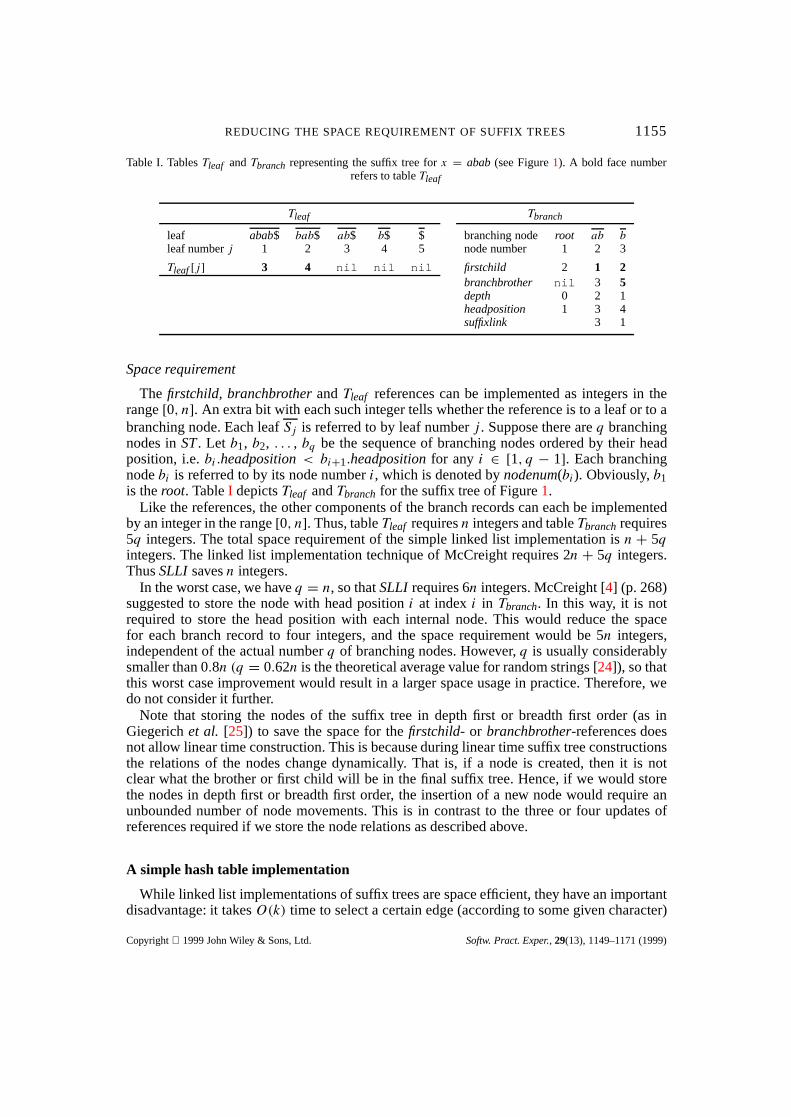
A simple linked list implementation

The simple linked list implementation technique (SLLI for short) representsST by twotablesTleaf andTbranchwhich store the following values: for eachleaf number j∈ [1, n+ 1],Tleaf[j ] stores a reference to the right brother of leafSj . If there is no such brother, then


1154 S. KURTZ

Figure 2. The references of the suffix tree forx = abab (see Figure1). Vertical arcs stand for firstchild references,and horizontal arcs for branchbrother andTleaf references

Tleaf[j ] is a nil reference. For each branching nodew, Tbranch[w] stores abranch recordconsisting of five componentsfirstchild, branchbrother, depth, headposition, andsuffixlinkwhose values are specified as follows:

1. firstchild refers to the first child ofw.2. branchbrotherrefers to the right brother ofw. If there is no such brother, then

branchbrotheris a nil reference.3. depthis the depth ofw.4. headpositionis the head position ofw.5. suffixlink refers to the branching nodev, if w is of the formav for somea ∈ 6 and

somev ∈ 6∗.The successors of a branching node are therefore found in a list whose elements are linked

via thefirstchild, branchbrotherandTleaf references. To speed up the access to the successors,each such list is ordered according to the first character of the edge labels. Figure2 shows thechild and brother references of the nodes of the suffix tree of Figure1. We use the followingnotation to denote a record component: for any componentc and any branching nodew,w.cdenotes the componentc stored in the branch recordTbranch[w]. Note that the head positionj of some branching nodewu tells us that the leafSj occurs in the subtree below nodewu.Hence,wu is the prefix ofSj of lengthwu.depth, i.e. the equalitywu = xj . . . xj+wu.depth−1holds. As a consequence, the label of the incoming edge to nodewu can be obtained bydropping the firstw.depthcharacters ofwu, wherew is the predecessor ofwu:

Observation 3 If wu→ wu is an edge inST andwu is a branching node, thenu =

xi . . . xi+l−1 wherei = wu.headposition+w.depthandl = wu.depth− w.depth.

Similarly, the label of the incoming edge to a leaf is determined from the leaf number andthe depth of the predecessor:

Observation 4 If wu→ wu is an edge inST andwu = Sj for somej ∈ [1, n + 1], then

u = xi . . . xn$, wherei = j + w.depth.

A similar observation was made by Larsson [23], but without a clear statement aboutits consequences concerning the space requirement ofST. Note that storing the depth of abranching node has some practical advantages over storing the length of the incoming edgeto a node (the latter is suggested by McCreight [4]). At first, during the sequential suffix treeconstructions [4,19,20], the depth of a node never changes. So it is not necessary to update thedepth of a node (the same is true for the head position). Second, the depth of the nodes along achain of suffix links is decremented by one, a property which can be exploited to store a suffixtree more space efficiently, see the next section. The third advantage of storing the depth isthat several applications of suffix trees assume that the depth of a node is available [3].



Table I. TablesTleaf andTbranch representing the suffix tree forx = abab (see Figure1). A bold face numberrefers to tableTleaf

Tleaf Tbranch

leaf abab$ bab$ ab$ b$ $ branching node root ab bleaf numberj 1 2 3 4 5 node number 1 2 3

Tleaf[j ] 3 4 nil nil nil firstchild 2 1 2branchbrother nil 3 5depth 0 2 1headposition 1 3 4suffixlink 3 1

Space requirement

The firstchild, branchbrotherandTleaf references can be implemented as integers in therange[0, n]. An extra bit with each such integer tells whether the reference is to a leaf or to abranching node. Each leafSj is referred to by leaf numberj . Suppose there areq branchingnodes inST. Let b1, b2, . . . , bq be the sequence of branching nodes ordered by their headposition, i.e.bi.headposition< bi+1.headpositionfor any i ∈ [1, q − 1]. Each branchingnodebi is referred to by its node numberi, which is denoted bynodenum(bi). Obviously,b1is theroot. TableI depictsTleaf andTbranch for the suffix tree of Figure1.

Like the references, the other components of the branch records can each be implementedby an integer in the range[0, n]. Thus, tableTleaf requiresn integers and tableTbranchrequires5q integers. The total space requirement of the simple linked list implementation isn + 5qintegers. The linked list implementation technique of McCreight requires 2n + 5q integers.ThusSLLI savesn integers.

In the worst case, we haveq = n, so thatSLLI requires 6n integers. McCreight [4] (p. 268)suggested to store the node with head positioni at indexi in Tbranch. In this way, it is notrequired to store the head position with each internal node. This would reduce the spacefor each branch record to four integers, and the space requirement would be 5n integers,independent of the actual numberq of branching nodes. However,q is usually considerablysmaller than 0.8n (q = 0.62n is the theoretical average value for random strings [24]), so thatthis worst case improvement would result in a larger space usage in practice. Therefore, wedo not consider it further.

Note that storing the nodes of the suffix tree in depth first or breadth first order (as inGiegerichet al. [25]) to save the space for thefirstchild- or branchbrother-references doesnot allow linear time construction. This is because during linear time suffix tree constructionsthe relations of the nodes change dynamically. That is, if a node is created, then it is notclear what the brother or first child will be in the final suffix tree. Hence, if we would storethe nodes in depth first or breadth first order, the insertion of a new node would require anunbounded number of node movements. This is in contrast to the three or four updates ofreferences required if we store the node relations as described above.

A simple hash table implementation

While linked list implementations of suffix trees are space efficient, they have an importantdisadvantage: it takesO(k) time to select a certain edge (according to some given character)


1156 S. KURTZ

outgoing from a node. If the alphabet is large this may slow down suffix tree constructionsand traversals considerably. Using balanced search trees instead of linked lists would improveworst case access toO(logk). However, with the additional overhead and the additionalspace requirement it is not clear whether this would improve the running time in practice.For this reason, we consider hashing techniques. McCreight [4] already suggested these forthe implementation of suffix trees.

We found the following simple hash table implementation technique (SHTI, for short) towork well in practice: for each edgew

av→ wavone stores the node number ofwav in a hashtable using the pair (w.headposition, a) as a hash key. Given a nodew and some charactera,the hash table allows to check whether there is ana-edge outgoing fromw. In case such anedge exists, sayw

av→ wav, a reference towav is delivered, as well as the edge labelav.

Space requirement

The number of edges is bounded by 2n, so a hash table of size 2n suffices. Besides thehash table, there is a table storing a record for each branching node. Such a record consistsof the three componentsdepth, headpositionand suffixlink, as defined above, and so thistable requires 3q integers. The space requirement for the hash table depends on the hashingtechnique. We use an open addressing hashing technique, with double hashing [26] to resolvecollisions. The hash function is based on the division method. This implies that the actual sizeof the hash table is the smallest prime larger than 2n. Each entry of the hash table stores twointegers: the hashed value and the left component of the hash key. It is not necessary to storethe right component of the hash key (i.e. the character), since this can be retrieved in constanttime, provided the depth of the node the edge is outgoing from is known; see Observations 3and 4. The hash table thus requires 4n integers, which means that the total space requirementof SHTI is 4n+ 3q integers.

Note that McCreight recommends to use Lampson’s hashing technique (see Knuth [26],section 6.4, p. 543, and Example 13), which belongs to the class of chaining techniques.This hashing technique uses an overflow area and a linked list of synonyms, and saves spaceby only storing the remainder of the key. However, as remarked by Cleary [27], each hashtable entry (including the original hash location) requires a reference to the next overflowrecord. This reference will be of about the same size as the reduction in the key size. So,Lampson’s hashing technique does not lead to net memory space savings over the openaddressing technique we used. In other words, the latter is the better choice.

We considered other hashing and tree implementation methods, which are, however, notapplicable to suffix trees without severe performance penalties:

(a) Compact Hashing [27] allows to store hash tables in a more space efficient way, byabbreviating a hash key (which we already did by only storing one component of thehash key). It requires randomizing hash keys, which can be very time consuming inpractice.

(b) TheBonsai implementation technique [28] is based on Compact Hashing, while thedouble-array technique [29,30] combines the advantages of arrays and lists. Bothtechniques are specifically designed to represent trees space efficiently. However, theyboth required the tree to be built from the root downward, a precondition which is notmet by any of the linear time suffix tree construction methods [4,19,20,21].



REVEALING AND EXPLOITING REDUNDANCIES

Small nodes and large nodes

We now show that the information stored for the branching nodes of the suffix tree containsredundancies. We reveal these by studying properties of the head positions. This leads to arelation between node numbers and suffix links.

Observation 5

1. If u andw are different branching nodes, thenu.headposition6= w.headposition.2. For any branching nodeaw in ST, w is also a branching node inST. Moreover, the

inequalityaw.headposition+ 1≥ w.headpositionholds.

Observation 5 implies that for any branching nodeaw we either haveaw.headposition+1 = w.headpositionor aw.headposition> w.headposition. We discriminate all non-rootnodes accordingly:aw is asmallnode if and only ifaw.headposition+ 1= w.headposition.aw is alargenode if and only ifaw.headposition> w.headposition. Theroot is neither smallnor large. The following observation shows that a small node is always directly followed byanother branching node, and that the last branching node is a large node.

Observation 6 Let aw be a branching node inST. Then the following holds:

1. If aw is small, thennodenum(aw)+ 1= nodenum(w).2. If nodenum(aw) = q andq > 1, thenaw is large.

According to Observation 6, we can partition the sequenceb2, . . . , bq of branching nodesinto chainsof zero or more consecutive small nodes followed by a single large node: achainis a contiguous subsequencebl, . . . , br , r ≥ l, of b2, . . . , bq such that the following holds:

(a) bl−1 is not a small node.(b) bl, . . . , br−1 are small nodes.(c) br is a large node.

One easily observes that any branching node (except for theroot) in ST is a member ofexactly one chain. The branch records for the small nodes of a chain store some redundantinformation, as shown in the following observation:

Observation 7 Letbl, . . . , br be a chain. The following properties hold for anyi ∈ [l, r−1]:1. bi.depth= br.depth+ (r − i).2. bi.headposition= br.headposition− (r − i).3. bi.suffixlink= bi+1.

We now show how to exploit these redundancies to store the information in the branchingnodes in less space. Consider a chainbl, . . . , br . Observation 7 shows that it is not necessaryto storebi.depth, bi.headpositionandbi.suffixlink for any i ∈ [l, r − 1]: bi.suffixlinkrefersto the next node in the chain, and if the distancer − i of the small nodebi to the large nodebr (denoted bybi.distance) is known, thenbi.depthandbi.headpositioncan be obtained inconstant time. This observation leads to the following implementation technique.


1158 S. KURTZ

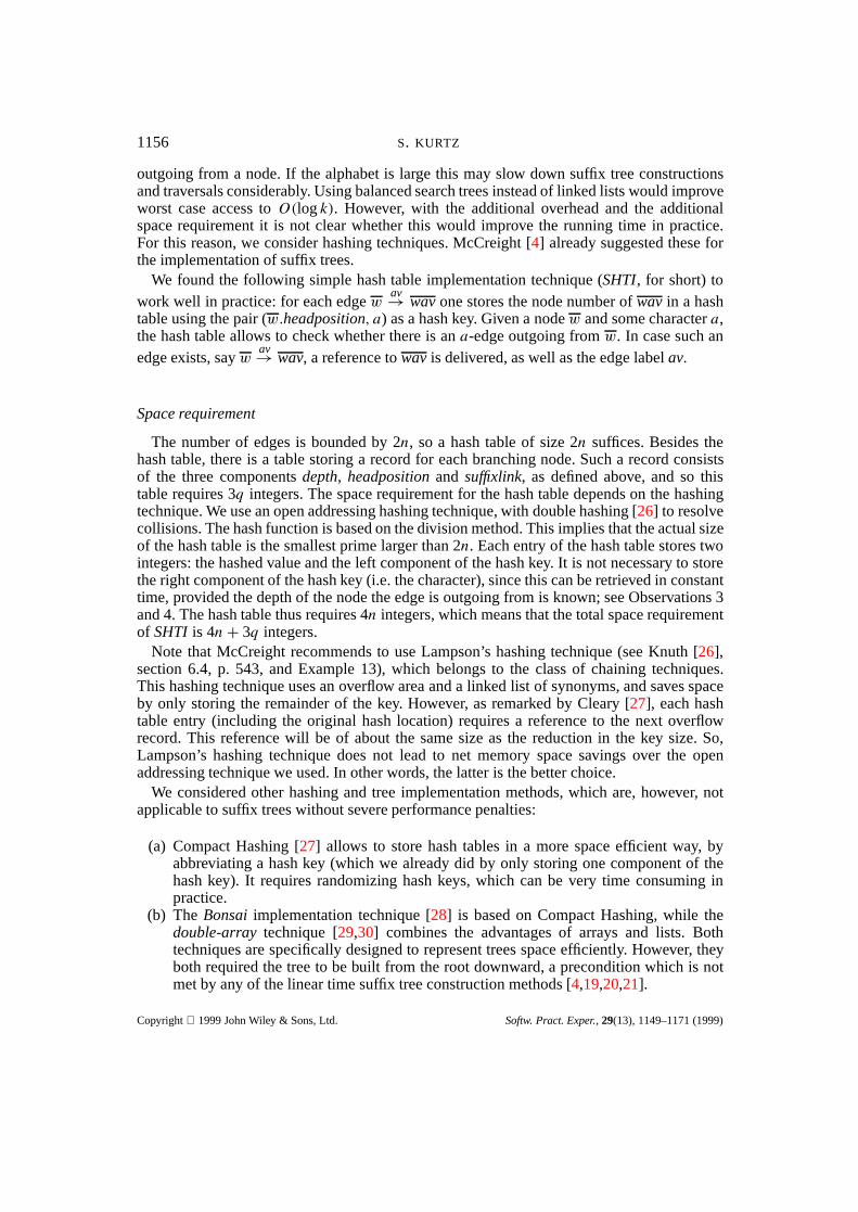
Table II. The tableT ′branch for the suffix tree forx = abab(see Figure1). A small record is stored in two integers

and a large record in four integers.ab is a small node with head position 3, andb is a large node with head position4. Both form a chain. The distance ofab andb is 1, depicted as a tiny 1 in the small record forab. Consider thelarge record forb: the tiny 0 stands for the unused most significant bits of the first integer, and the third integer

stores the small depth (to the right) and the suffix link (to the left). A bold face number refers toTleaf

5 nil 0 1 1 1 8 0 2 5 0 1 4︸︷︷︸︸︷︷︸︸︷︷︸root ab b

An improved linked list implementation

The improved linked list implementation (ILLI , for short) representsST by two tablesTleaf andT ′branch. Tleaf is as inSLLI. TableT ′branch stores the information for the small andthe large nodes: for each small nodew, there is asmall recordwhich storesw.distance,w.firstchild andw.rightbrother. For each large nodew there is alarge recordwhich storesw.firstchild, w.rightbrother, w.depthandw.headposition. Wheneverw.depth≤ 2α − 1, forsome constantα, we say that the large record forw is complete. A complete large recordalso storesw.suffixlink. A large nodew with w.depth> 2α − 1 is handled as follows: letv be the rightmost child ofw. There is a sequence consisting of onefirstchild referenceand at mostk − 1 rightbrother/Tleaf references which linkw to v. If v = Sj for somej ∈ [1, n + 1], thenTleaf[j ] is a nil reference. Otherwise, ifv is a branching node, thenv.rightbrother is a nil reference. Of course, it only requires one bit to mark a reference asa nil reference. Hence the integer used for the nil reference contains unused bits, in whichw.suffixlinkis stored. As a consequence, retrieving the suffix link ofw requires traversing thelist of successors ofw until the nil reference is reached, which encodes the suffix link ofw.This linear retrievalof suffix links takesO(k) time in the worst case. However, despite linearretrieval, the suffix tree can still be constructed inO(kn) time, since the suffix link is retrievedat mostn times during suffix tree construction [4,18]. Moreover, suffix tree applications whichutilize suffix links [3,31,32] have an alphabet factor in their running time anyway (if a linkedlist implementation of suffix trees is used). As a consequence, linear retrieval of suffix linksdoes not influence the asymptotic running time, neither of suffix tree constructions, nor ofsuffix tree applications. Recall that linear retrieval of suffix links is required only for largenodes whose depth exceeds 2α − 1. α will be chosen such that those nodes are usually veryrare. If they occur, then the number of successors is expected to be small, and hence linearretrieval of suffix links is fast.

To guarantee constant time access from a small nodebi to the large nodebr , the records arestored in tableT ′branch, ordered by the head positions of the corresponding branching nodes.All branching nodes are referenced by theirbase addressin T ′branch, i.e. the index of thefirst integer of the corresponding record. TableII depicts tableT ′branch for the suffix tree ofFigure1.

Space requirement

Suppose a base address can be stored inβ bits. A reference is either a base address or a leafnumber. To distinguish these, we need one extra bit. Thus a reference requires 1+β bits. Each



depth and each head position occupiesγ = dlog2 ne bits. Consider the range of the distancevalues. In the worst case, take for example,x = an, there is only one chain of lengthn− 1,i.e. the maximal distance value isn− 2. However, this case is very unlikely to occur. To savespace, we delimit the maximal length of a chain to 2δ for some constantδ. As a consequence,after at most 2δ−1 consecutive small nodes an ‘artificial’ large node is introduced, for whichwe store a large record. In this way, we delimit the distance value to be at most 2δ − 1, andthus the distance occupiesδ bits. Thus we trade a delimited distance value for the saving ofγ − δ bits for each small record.

A small record stores two references, a distance value, and onenil bit to mark a reference asa nil reference, which add up to 2·(1+β)+δ+1 = 3+2β+δ bits. A large record stores tworeferences, one nil bit, and onecomplete bitwhich tells whether the large node is complete.Moreover, there areγ bits required for the head position. If the record is complete thenβ bitsare used for the suffix link andα bits for the depth. Otherwise,γ bits are used for the depth.We leaveδ bits unused, i.e. they store the ‘distance’ 0. In this way, we can discriminate largeand small nodes, since the latter always have a positive distance value. Altogether a completelarge record requires 2· (1+ β) + 1+ 1+ γ + β + α + δ = 4+ 3β + γ + α + δ and anincomplete large record requires 2· (1+ β)+ 1+ 1+ 2γ + δ = 4+ 2(β + γ )+ δ bits.

To determine the actual space requirement we must choose the constantsδ and α andconsider the maximal length of the input string we allow. In our current implementation weassumen ≤ 227− 1 (which impliesγ = 27), and have chosenα = 10 andδ = 5. Thenwe can store a small record in two integers and reserve four integers for a large record.∗∗As a consequence the maximal base address is 4n − 4, and any base address is even. Henceβ = γ + 1, which means that a small record requires 3+ 2β + δ = 64 bits, i.e. two integers.An incomplete large record requires 4+2(β+γ )+δ = 119 bits, and a complete large recordrequires 4+ 3β + γ + α + δ = 130 bits. Both fit into four integers, if we store 2 bits for thelatter type of record inTleaf[w.headposition], wherew is the corresponding node. Recall thatTleaf[w.headposition] stores a reference (29 bits) and one nil bit.

Letσ be the number of small records andλ be the number of large records.T ′branchrequires2σ + 4λ integers. TableTleaf occupiesn integers, and hence the space requirement ofILLI isn+2σ +4λ integers. The implementation technique of McCreight [4] requires 2n+5(σ +λ)integers. Each leaf and each large node saves one integer, and each small node saves threeintegers. ThusILLI leads to large space savings, if there are many small nodes.

Example 1 Consider the input stringx = an. ThenST hasn − 2 small nodes, one largenode (i.e.a), and 2n edges. Hence the space requirement ofILLI is 3n+ 1

16n integers (thereare 2

32n extra integers required for the artificial large nodes). This is the best case. In contrast,the space requirement forSLLI is 6n, which is the worst case. HenceILLI requires about halfof the space used bySLLI.

Example 2 Consider the input stringx = aabbabaaababbaabaabbof length n = 20.Then ST contains 3 small nodes and 14 large nodes, and hence the space requirement is(20+3·2+15·4)/20= 4.3 integers per input character. This is the largest space requirementof ILLI for all strings of length 20 over the alphabet6 = {a, b}. The saving overSLLI is 24integers.

The last example shows that there can be many large nodes. We conjecture that the upperbound onλ occurs for binary alphabets and that it is around 0.7n, as in Example 2. However,

∗∗We assume that each integer occupies 32 bits. Note that this does not imply that the word size of the computer is 32 bits. Infact, the software constructing our suffix tree representations works on 32 bit as well as on 64 bit machines without any changes.


1160 S. KURTZ

we cannot prove this and have to calculate with an upper boundλ ≤ n.Note that the proposed suffix tree representations can be constructed in linear time without

extra space, by a slight modification of McCreight’s suffix tree algorithm [4]. The basicobservation is that this algorithm constructs the branching nodes ofST in order of theirhead positions, which is compatible with our implementation techniques. For details, seeKurtz [18].

An improved hash table implementation

The redundancy of the information stored in the branching nodes can also be exploitedto reduce the space requirement of the simple hash table implementation technique. In theimproved hash table implementation technique, referred to byIHTI , we usereference pairstoaddress the nodes ofST. In particular, each leafSj is addressed by the reference pair(0, j).Let l1, l2, . . . , lp be the sequence of large nodes inSTordered by their head position. This is asubsequence ofb1, b2, . . . , bq , the sequence of branching nodes, as defined above. Considerthe chain which ends with the large nodeli . li is referenced by the pair (1, i). Each small nodein this chain with distanced > 0 to li is referenced by the pair (d+1, i). Using these referencepairs, it suffices to store the large records. Thesuffixlink, theheadpositionand thedepthofeach small node can be retrieved in constant time, according to Observation 7, since thedistance to the large node of the chain is encoded in a reference pair. The hashing techniqueof the previous section only has to be slightly modified: consider the edgew

av→ wav, andsuppose thatwav is a node which is addressed by the reference pairp. Then one stores thepair (w.headposition, p) in the hash table using (w.headposition, a) as a hash key.

Another observation about the leaf edges allows us to reduce the size of the hash tableconsiderably. Note that for a nodew with head positioni there is often a leaf edgew

av→ Si .Let us call such a leaf edgeidentityedge.

Example 3 Consider the suffix tree for the stringabab. Then there are two identity edges

ab$→ ab$ andb

$→ b$, which can be easily deduced from TableI.

There is at most one identity edge outgoing from each branching node. The observationis that it is not necessary to explicitly store identity edges in the hash table. We just need asingle bit to mark that there is an identity edge outgoing from a branching node with headpositioni. Knowing this, we can deduce the leaf numberi, the identity edge leads to, as wellas the corresponding edge label, see Observation 4. For eachi ∈ [0, n], the ith entry of thehash table contains an unused bit. This can be used as a marking bit, so that no extra spaceis required to represent the identity edges. If we do not store the identity edges explicitly,then we can reduce the size of the hash table considerably. In fact, we have never found anyinput string for which the number of non-identity edges exceeds 1.5n. Hence we only use ahash table of size 1.5n. For the very unlikely situation that the hash table overflows, one canenlarge it and rehash all entries that are currently stored. Unfortunately, we cannot prove aworst case bound better than 2n for the size of the reduced hash table.

Space requirement

A reference pair is implemented by a single integer. We restrict the maximal length of thechains to 31 (one less than forILLI ). So the maximal distance value is 30, and the maximal



value in the left component of a reference pair is 31, i.e. it occupies 5 bits. This leaves 27 bitsfor storing the right component, i.e. the leaf number or the numberi of a large nodeli . As aconsequence, the length of the string to be processed is delimited to 227− 1= 134,217,727.The space requirement ofIHTI is thus 4n + 3λ integers. Therefore, the saving overSHTI is3σ integers.

Example 4 Consider the stringx = an. ThenSTcontainsn− 2 small and one large node.There are 2n edges,n of which are identity edges. Using a hash table of size 1.5n, the spacerequirement forIHTI is 3n+ 3

31n integers, which is almost identical to the space requirementof ILLI . The saving overSHTI is almost 4n integers.

Example 5 Consider the input stringx = aabbabaaababbaabaabbof Example 2. Thereare three small nodes, 14 large nodes, and 38 edges, 11 of which are identity edges. Using ahash table of size 30, the space requirement forIHTI is (2 · 30+ 3 · 15)/20= 5.25 integersper input character. The reduction in the size of the hash table saves 10 integers, and the threesmall nodes save nine integers overSHTI.

UPPER LIMITS ON THE INPUT STRING LENGTH

Usually, the memory available delimits the maximal length of the input string which can beprocessed. However, on some computers with very large memory, one also has to take intoaccount the available address space. This is delimited by 2ω − 1, whereω is the word size ofthe computer. The worst case space requirement ofILLI is 5n integers. With the additionalnbytes for representing the input string, the total space requirement is 21n bytes in the worstcase. Since 21(227− 1) = 2,818,572,267 is well below 232− 1, we can safely assume thatall bytes of the suffix tree representation ofILLI can be addressed on a computer with wordsizeω ≥ 32. In case strings longer than 227− 1 are to be processed (and enough memoryis available), one can modifyILLI such that each small and each large record contains anextra integer. This results in an implementation techniqueILLI ′ with a space requirement ofn+ 3σ + 5λ integers.

The improved hash table implementation has a worst case space requirement of 7n integers.Since 29(227 − 1) = 3,892,314,083 is well below 232 − 1, all bytes can be addressed,wheneverω ≥ 32. For the other implementation techniques and compactdawgs, the upperlimit on n is (2ω−1)/wcs, wherewcsis the worst case space requirement in bytes (includingthe n bytes for the input string). In practice, this number is actually smaller since there isa constant amount of memory required for the operating system and program execution.TableIII gives an overview of the space requirements and the upper limits onn for ω = 32.

EXPERIMENTS

For our experiments we collected a set of 42 files (total length 18,684,070) from differentsources:

(a) We used 17 files from the Calgary Corpus and all 14 files from the CanterburyCorpus [33]. The Calgary Corpus usually consists of 18 files, but since the filepicis identical to the fileptt5 of the Canterbury Corpus, we did not include it here. Bothcorpora are widely used to compare lossless data compression programs.


1162 S. KURTZ

Table III. Overview of the space requirement of different suffix tree implementation techniques and compactdawgs. n is the length of the input string,σ is the number of small nodes, andλ is the number of large nodesin the suffix tree. The worst case space requirement is calculated by substituting 0 forσ andn for λ. s is thenumber of states andt is the number of transitions in the compactdawg. The worst case occurs for the input stringx = an−1b: thens = n andt = 2n− 2. Since each state and each edge occupies three integers [6], the worst casespace requirement of compactdawgs is 36n bytes. For calculating the upper bounds we addedn bytes which are

required to represent the input string

Space (in integers) Upper limit onn for ω = 32

McCreight 2n+ 5(σ + λ) (232− 1)/29= 148,102,320SLLI n+ 5(σ + λ) (232− 1)/25= 171,798,691SHTI 4n+ 3(σ + λ) (232− 1)/29= 148,102,320ILLI n+ 2σ + 4λ 227− 1= 134,217,727ILLI ′ n+ 3σ + 5λ (232− 1)/25= 171,798,691IHTI 3(n+ λ) 227− 1= 134,217,727Compact dawgs 3(s + t) (232− 1)/37= 116,080,197

(b) We added eight DNA sequences used by Lefévre and Ikeda [15]. These are denoted bytheir EMBL database accession number.

(c) We extracted a section of 500,000 residues from the PIR database, denoted byPIR500.The underlying alphabet is of size 20.

(d) We generated two random stringsR500k4 andR500k20 of length 500,000 over analphabet of size 4 and over an alphabet of size 20. The characters are drawn with uniformprobability.

Space requirement

We compared the space requirement of the described implementation techniques with thespace requirement of variants of directed acyclic word graphs [12,13]. To obtain concretenumbers, we developed software to computedawgs. Given adawg, it is fairly easy to computethe number of nodes and edges in the correspondingposition end-set treeof Lefevre andIkeda [15] (pestry, for short). The same holds for thecompact dawg[14] (cdawg, for short).A tight implementation of adawg and apestry, based on linked lists, requires nine bytesfor each node and eight bytes for each edge. For thecdawg, 12 bytes are required for eachnode and for each edge. These numbers are consistent with Crochemore and Vérin [6]. Wealso counted the number of small and large nodes in the suffix trees to calculate the spacerequirement for the different suffix tree implementation techniques, according to the formulasgiven in TableIII .

TableIV shows the relative space requirement (in bytes per input char) of thedawg, thepestry, the cdawg, and for suffix trees using the implementation technique of McCreight(McC) and the improved implementation techniquesILLI and IHTI we propose. Weemphasize that the given numbers refer to the space required for construction. It doesnotinclude then bytes used to store the input string.

The first column of TableIV shows the name of the file and the second its source, as far as ithas not been made precise above:CL stands for the Calgary Corpus,CN for the CanterburyCorpus, andEM for the EMBL data base. In addition, a single character denotes the type of



Table IV. Relative space requirement (in bytes/input char) ofdawgs and suffix trees

File Source Length k dawg pestry cdawg McC ILLI IHTI

book1 CL/e 768771 81 30.35 19.97 15.75 18.02 9.83 14.73book2 CL/e 610856 96 29.78 17.92 12.71 18.63 9.67 14.13paper1 CL/e 53161 95 30.02 18.12 12.72 18.92 9.82 14.17paper2 CL/e 82199 91 29.85 18.53 13.68 18.51 9.82 14.42paper3 CL/e 46526 84 30.00 19.00 14.40 18.28 9.80 14.53paper4 CL/e 13286 80 30.34 19.50 14.76 18.35 9.91 14.66paper5 CL/e 11954 91 30.00 18.86 14.04 18.41 9.80 14.46paper6 CL/e 38105 93 30.29 18.28 12.80 19.07 9.89 14.19alice29 CN/e 152089 74 30.27 18.90 14.14 18.63 9.84 14.38lcet10 CN/e 426754 84 29.75 17.84 12.70 18.61 9.66 14.12plrabn12 CN/e 481861 81 29.98 19.65 15.13 17.84 9.74 14.71bible CN/e 4047392 63 29.28 16.75 10.87 16.10 7.27 12.04world192 CN/e 2473400 94 27.98 14.55 7.87 18.81 9.22 13.35bib CL/f 111261 81 28.53 15.88 9.94 18.76 9.46 13.73news CL/f 377109 98 29.48 17.58 12.10 18.41 9.54 14.06progc CL/f 39611 92 29.73 17.42 11.87 18.69 9.59 13.97progl CL/f 71646 87 29.96 16.27 8.71 20.98 10.22 13.55progp CL/f 49379 89 30.21 16.24 8.28 21.39 10.31 13.43trans CL/f 93695 99 30.47 15.97 6.69 22.22 10.49 13.21fieldsc CN/f 11150 90 29.86 16.39 9.40 19.81 9.78 13.59cp CN/f 24603 86 29.04 16.64 10.44 18.41 9.34 13.76grammar CN/f 3721 76 29.96 17.17 10.60 20.2510.14 13.85xargs CN/f 4227 74 30.02 18.50 13.10 18.15 9.63 14.35asyoulik CN/f 125179 68 29.97 19.46 14.93 18.02 9.77 14.64geo CL/b 102400 256 26.97 19.09 13.10 13.41 7.49 13.99obj1 CL/b 21504 256 27.51 16.68 13.20 14.53 7.69 13.61obj2 CL/b 246814 256 27.22 14.23 8.66 18.81 9.30 13.46ptt5 CN/b 513216 159 27.86 13.71 8.08 19.17 8.94 12.71kennedy CN/b 1029744 256 21.18 8.35 7.29 9.10 4.64 12.31sum CN/b 38240 255 27.79 14.85 10.26 17.65 8.92 13.58ecoli CN/d 4638690 4 34.01 27.34 23.55 20.8412.56 17.14J03071 EM/d 66495 4 33.70 20.47 13.44 24.1412.36 14.85K02402 EM/d 38059 4 34.12 27.60 23.90 20.8312.59 17.18M13438 EM/d 2657 4 33.95 27.59 23.96 20.6512.50 17.16M26434 EM/d 56737 4 34.10 26.51 22.52 21.3812.52 16.75M64239 EM/d 94647 4 34.10 27.60 23.94 20.8712.62 17.20V00636 EM/d 48102 4 34.02 27.75 24.04 20.7212.57 17.22V00662 EM/d 16569 4 34.14 27.61 24.10 20.9012.69 17.29X14112 EM/d 152261 4 34.13 27.12 23.43 21.1212.58 17.00PIR500 500000 20 30.35 22.70 15.79 17.51 9.87 15.09R500k4 500000 4 33.93 28.06 24.15 20.4412.56 17.38R500k20 500000 20 29.83 27.98 20.06 14.939.40 15.94

Average relative space requirement for all files 30.33 19.78 14.55 18.82 10.10 14.66

Average relative space requirement for DNA 34.03 26.62 22.54 21.27 12.55 16.86


1164 S. KURTZ

the file:e for english text,f for formal text (like programs),b for binary files (i.e. containing8-bit characters), andd for DNA sequences. Columns three and four show the lengths andthe alphabet sizes. In each row, the smallest relative space requirement is shown in boldface.The last two rows show the average relative space requirement for all files and for all DNAsequences. In the following, when we write space requirement we mean average relative spacerequirement.

There are some interesting findings which can be derived from TableIV. Since DNAsequences are very important for suffix tree applications, we in particular comment on thecorresponding behavior of the considered data structures:

1. Thedawgis the least space efficient data structure.2. Thepestryrequires about 35 per cent less space than thedawg. For DNA sequences the

saving over thedawg is 22 per cent. This is slightly smaller than the saving of 25–30per cent reported by Lefévre and Ikeda [15].

3. A cdawgrequires on average 26 per cent less space than apestry. For DNA sequencesthe saving over thepestryis 15 per cent. As suggested by Crochemore and Vérin [6],the space requirement of thecdawgfor DNA sequences can be reduced by using arraysinstead of linked lists to represent outgoing edges. This results in an implementationreferred to bycdawgA. It requires 20.66n bytes for the DNA sequences we used. Thisis consistent with the numbers given by Crochemore and Vérin [6]. For alphabets largerthan four,cdawgAdoes not make sense. In some cases, in particular for formal texts, thecdawgis the most space efficient data structure. Note that its space requirement variesvery much between 6.69n bytes and 24.15n bytes.

4. The suffix tree in the implementation following McCreight uses 30 per cent more spacethan thecdawg. However, for all DNA sequences, except for J03071, it requires lessspace than thecdawg. For DNA sequences the saving over thecdawgis 6 per cent, butit uses 3 per cent more space than thecdawgA.

5. The suffix tree in the improved linked list implementation is the most space efficientdata structure. It improves over thecdawgby 30 per cent and overMcC by 46 percent. For all classes of files there is an advantage over thecdawg. However, there areseven files for which thecdawgrequires less space. For DNA sequences the savingover thecdawgand thecdawgAis 44 per cent and 39 per cent, respectively. The spacerequirement varies between 4.64n bytes and 12.69n bytes. Thus the upper bound on thespace requirement is 11.45n bytes smaller than the upper bound for thecdawg.

6. The suffix tree in the improved hash table implementation requires 45 per cent morespace than the suffix tree in the improved linked list implementation. The spaceconsumption is similar to thecdawgand it improves overMcC by 22 per cent. ForDNA sequences the space requirement is 16.86n bytes, which is an improvement overthe cdawgandcdawgAof 25 per cent and 18 per cent. The space requirement variesbetween 12.31n bytes and 17.38n bytes.

Figure3 presents the data of TableIV in a more compact way. For each type of file (exceptrandom) and each of the considered data structures and implementation techniques, a columnshows the average relative space requirement for all files of that type. For DNA sequences wehave seven columns, where the last column refers tocdawgA. It is obvious that the size of thedata structures depends upon the kind of input data: binary strings lead to the smallest datastructures, for formal text and english text all data structures are slightly larger. For proteinsequences and in particular DNA sequences the space requirement is considerably higher.



Figure 3. Relative space requirement (in bytes/input char) of dawgs and suffix trees for five groups of files

Running time

For our second experiment we implemented four different variants of McCreight’s suffixtree construction named after the implementation technique they employ:SLLI,SHTI, ILLIandIHTI . All programs are written in C. We compiled our programs with thegcc compiler,version 2.8.1, with optimizing option –O3. The programs were run on aSun-UltraSparc,300 MHz, 192 megabytes RAM under Solaris 2. TableV shows the lengths of the files andthe alphabet sizes. Columns 4–11 present the running times of the four programs:absoluteuser runningtimeandrelativeuser running timertime= (106 · time)/n, i.e. the time requiredto process 106 characters. Times are in seconds, as measured by thegnu timeutility, averagedover 1000, 100 or 10 runs, depending on the size of the files. The last row shows the totalrunning time and the average relative running time. In each line the smallest relative runningtime is shown in boldface.

TableV shows that the simple implementation techniques lead to slightly faster programsthan the improved implementation techniques. However, the running time advantage ofthe simple implementation techniques are very small: 2 per cent for the linked listimplementation, and 1.5 per cent for the hash table implementation. So, the additionalconstant overhead for the improved but more complicated implementation techniques areworth the effort.

Comparing the linked list implementations with the hash table implementations, oneobserves that the former are faster if the alphabet is small (i.e.k ≤ 100) and if the inputstring is short (i.e.n ≤ 150,000). We explain this as follows: the most time consuming partof the linked list implementation is traversing the list of successors of a particular node. Eachsuch traversal step requires only a few very simple and fast operations. But the nodes accessedduring such a traversal may be stored at very distant locations in memory, which means thatMcCreight’s algorithm has a poor locality behavior [34]. If the text is short, then the entiresuffix tree representation usually fits into the cache, so that cache misses are rare. So the poorlocality does not matter, and hence the good performance of the linked list implementationsfor the case that the alphabet and the text are small. For larger files one clearly observes thatthe linked list implementation becomes slower, independent of the alphabet size.


1166 S. KURTZ

Table V. Running times (absolute and relative in seconds) for different variants of McCreight’s algorithm

SLLI ILLI SHTI IHTI

File Length k Time Rtime Time Rtime Time Rtime Time Rtime

book1 768771 81 3.40 4.42 3.75 4.88 2.58 3.35 2.66 3.46book2 610856 96 2.21 3.61 2.33 3.82 1.94 3.18 1.903.10paper1 53161 95 0.10 1.95 0.11 2.05 0.13 2.41 0.12 2.20paper2 82199 91 0.19 2.26 0.18 2.22 0.23 2.74 0.23 2.83paper3 46526 84 0.09 2.02 0.09 1.97 0.11 2.30 0.10 2.20paper4 13286 80 0.02 1.71 0.03 1.93 0.02 1.73 0.02 1.84paper5 11954 91 0.02 1.81 0.02 1.73 0.02 1.73 0.02 1.98paper6 38105 93 0.07 1.79 0.07 1.81 0.08 2.20 0.09 2.43alice29 152089 74 0.43 2.85 0.41 2.67 0.44 2.91 0.42 2.74lcet10 426754 84 1.44 3.37 1.46 3.42 1.33 3.11 1.272.97plrabn12 481861 81 1.87 3.88 2.00 4.16 1.56 3.24 1.563.23bible 4047392 63 15.33 3.79 15.70 3.88 14.01 3.46 13.553.35world192 2473400 94 9.19 3.72 8.96 3.62 7.50 3.03 7.252.93bib 111261 81 0.25 2.27 0.23 2.10 0.29 2.63 0.28 2.51news 377109 98 1.82 4.84 1.79 4.74 1.13 3.00 1.092.90progc 39611 92 0.07 1.69 0.07 1.80 0.09 2.18 0.08 1.97progl 71646 87 0.11 1.60 0.12 1.64 0.19 2.72 0.17 2.43progp 49379 89 0.07 1.45 0.07 1.43 0.12 2.46 0.11 2.14trans 93695 99 0.15 1.62 0.15 1.60 0.27 2.85 0.23 2.47fieldsc 11150 90 0.01 1.04 0.01 1.24 0.02 1.64 0.02 1.69cp 24603 86 0.03 1.39 0.04 1.61 0.04 1.63 0.04 1.67grammar 3721 76 0.004 0.98 0.004 1.18 0.006 1.62 0.006 1.63xargs 4227 74 0.004 1.06 0.006 1.43 0.006 1.53 0.007 1.67asyoulik 125179 68 0.32 2.54 0.32 2.58 0.36 2.84 0.34 2.72geo 102400 256 0.69 6.75 0.68 6.69 0.212.04 0.23 2.28obj1 21504 256 0.04 1.70 0.04 2.04 0.03 1.43 0.03 1.59obj2 246814 256 0.97 3.91 0.98 3.97 0.72 2.93 0.682.77ptt5 513216 159 0.91 1.77 0.88 1.70 1.44 2.80 1.22 2.37kennedy 1029744 256 16.16 15.70 16.76 16.27 1.261.22 1.63 1.58sum 38240 255 0.07 1.94 0.10 2.59 0.08 1.98 0.071.72ecoli 4638690 4 17.73 3.82 18.07 3.90 17.393.75 20.47 4.41J03071 66495 4 0.10 1.50 0.10 1.45 0.17 2.51 0.16 2.39K02402 38059 4 0.05 1.37 0.06 1.51 0.08 2.01 0.08 2.22M13438 2657 4 0.003 1.02 0.003 1.21 0.004 1.42 0.005 1.74M26434 56737 4 0.09 1.60 0.09 1.62 0.13 2.35 0.14 2.43M64239 94647 4 0.19 1.97 0.18 1.92 0.25 2.61 0.27 2.85V00636 48102 4 0.07 1.55 0.08 1.63 0.11 2.23 0.12 2.41V00662 16569 4 0.02 1.19 0.03 1.66 0.03 1.58 0.03 1.87X14112 152261 4 0.34 2.25 0.34 2.23 0.42 2.78 0.47 3.09PIR500 500000 20 3.07 6.14 3.22 6.44 1.62 3.25 1.68 3.35R500k4 500000 4 1.69 3.37 1.56 3.11 1.56 3.12 1.82 3.63R500k20 500000 20 3.68 7.36 3.90 7.80 1.482.95 1.62 3.24

83.09 2.92 84.98 3.03 59.44 2.46 62.28 2.50



The dominating factor for the hash table implementations is the modulo operation(remember that we use division hashing). On the machine we used, this operation is slowerthan addition by an order of magnitude. However, for large files, the slow modulo operationsare compensated for by the slow paging operations of the memory subsystem required by thelinked lists implementation, so that the hash table implementations become faster.

CONCLUSION

Applications

The main topic of this paper was to show that suffix trees can be implemented inmuch less space than previously thought. This should make suffix trees more attractive forpractical applications. Indeed, we have already used our implementation techniques in twoapplications:

(a) In a lossless data compression program [35], suffix trees in both improvedimplementation techniques are used to compute the Burrows and WheelerTransformation [36] of a string in linear time and space. This basically means to sort allsuffixes of a string in lexicographic order; see also TableIV, application 13.

(b) In a program calledREPuter[37], suffix trees in the improved linked list implementationare used to compute maximal repeats in DNA sequences in optimal time. We used analgorithm described by Gusfield [3] (see TableIV, application 11). With the improvedlinked list implementation we are able to compute all 174,187 maximal repeats of lengthat least 20 contained in the entire yeast genome (n = 12,147,818) in 68 seconds, using160 megabytes of space (Sun-UltraSparc, 300 MHz, 192 megabytes RAM). On thebasis of the average relative space requirement for DNA sequences (see the section on‘Experiments’), we can estimate the corresponding space requirement forcdawgAandMcCreight’s implementation technique with(20.66·12,147,818)/220≈ 240 megabytesand(21.27 · 12,147,818)/220 ≈ 246 megabytes, respectively. This does not fit into themain memory of the machine we used, and so very time consuming memory swapswould be required. These are not necessary whenILLI is used.

A suffix tree for the human genome

We now develop a conjecture about the resources required for computing the suffix treefor the complete human genome. The size of the human genome is estimated to be about3 · 109. We assume a computer with 64 bit architecture, so the address space is large enough.We modify implementation techniqueILLI such that each small node is represented by threeintegers, each large node occupies 5 integers, and tableTleaf consists ofn + 1 entries eachoccupying 1.25 integers. This leaves enough space to store references in the range[0,5n],wheren ≤ 232− 1. For the DNA sequences we used in our experiments, we determined theaverage ratiosσ/n = 0.258 andλ/n = 0.406. We now assume that for the human genome,the same ratios hold. Based on this assumption we estimate that the suffix tree for the completehuman genome will require about 3·109 · (1.25+3 ·0.258+5 ·0.406) = 1.22·1010 integersor 4 · 1.22 · 1010/230 = 45.31 gigabytes of main memory. Conservatively estimating that ourprogram requires 10 seconds to process one million characters, we obtain a running time ofabout 3· 104 seconds, which is less than nine hours. Given that sequencing of the completehuman genome is probably not finished before December 2001 and taking into account the


1168 S. KURTZ

Table VI. Applications of suffix trees and the kind of traversal they require. The numbers are the applicationnumbers used by Gusfield [3]

Applications with partial traversals Applications with complete traversals

1 exact string matching 4 longest common substring of two strings2 exact set matching 5 recognizing DNA contamination3 substring problem for a data base of patterns 6 common substrings to more than two strings8 computing matching statistics 7 building a smaller directed graph for exact9 space efficient longest common substring matching

problem 10 all pairs suffix prefix matching15 Boyer-Moore approach to exact set matching 11 finding maximal repetitive structures16 Ziv-Lempel data compression 12 circular string linearization17 Minimum length encoding of DNA 13 computing suffix arrays

expected advances in hard-ware technology, it seems feasible to compute the suffix tree for theentire human genome on some computers. This would be very helpful for genomic research.

Pragmatics of the choice between ILLI and IHTI

We described two basic implementation techniques to implement suffix trees: linked listsand hash tables. The experiments suggest that the choice of the implementation techniquedepends on (i) the alphabet size, (ii) the length of the input string, and (iii) whether spacerequirement or running time is more important. However, there is another important point toconsider: we have to take into account the way in which the suffix tree is utilized. There arebasically two ways to utilize a suffix tree:

1. The suffix tree is partially traversed according to some given string, e.g. a pattern. Thistask requires to decide for a given nodew and charactera whether there is ana-edgeoutgoing fromw, and in case such an edge exists, to deliver this edge.

2. The suffix tree is traversed completely in a particular order. This task requires to haveconstant time access from one edgev

aw→ vaw to another edgevcu→ vcu which has not

been traversed before (if such an edge exists). Sometimes this edge has to be the nextedge w.r.t. to some ordering on the first characters of the edge labels.

Partial traversals (see 1) are typical for pattern matching applications, and complete traversals(see 2) are typical for finding repetitive elements in strings. To give concrete examples weconsidered the first 17 applications of suffix trees given by Gusfield [3], and associatedthem according to whether they partially or completely traverse a suffix tree. Application 14(i.e. suffix trees in genome scale projects) subsumes several different applications, and so itcannot uniquely be associated with any of the two kinds. In the remaining 16 applications wehave found eight applications which perform partial traversals and eight applications whichperform complete traversals. TableVI lists the applications and their association.

Partial traversals can be accomplished with both basic implementation techniques.However, when using a linked list implementation this leads to an alphabet factor in therunning time. So, for partial traversals it is usually better to use a hash coded implementation,unless space is at the premium. Complete traversals can easily be accomplished with thelinked list implementation. In contrast, the hash table implementation is less useful here,



since it does not immediately reveal the set of edges outgoing from some node. As notedby Larsson [38], it is possible to sort the hash table such that it allows complete traversals.In a first phase all edges stored in the hash table are sorted according to the nodes they areoutgoing from. This can be done in time linear in the size of the hash table, i.e. inO(n),using a bucket sort algorithm. This requires at mostn extra integers to hold the counts foreach node. After the first phase, for each node the edges outgoing from that node are storedin consecutive positions of the hash table. These can be sorted inO(n) time altogether, againusing a bucket sort algorithm. Thus the extra sorting phase requiresO(n) time andn integersof extra space. We have implemented such a sorting procedure forIHTI . Unfortunately, itproved to be slow in practice: the running time of the additional sorting phase is between27 per cent and 140 per cent of the running time of the corresponding suffix tree construction(average 73 per cent). So, for complete traversals, the hash table representation is inferior,except when the alphabet is large.

Further improvements and analyses

We note that our implementation techniques are not optimized for a particular alphabet size.For DNA sequences, which lead to the largest index structures (see Figure3), there are somefurther optimizations possible: ifx is a DNA sequence, we can expect that each substringof lengthq ≤ log4 n over the DNA alphabet occurs at least twice. This means that most ofthe possible nodes of depth≤ q − 1 occur in the suffix tree, and these can be representedmore space efficiently using a heap. A similar technique has already been applied for hashedposition trees [16].

Finally, note that the proposed implementation techniques lead to some interestingcombinatorial questions: what is the expected number of small and large nodes? Are therebetter worst case bounds for the number of large nodes? What is the largest/expected numberof non-identity edges? Solutions to these problems definitely improve the acceptance of ourimplementation techniques.

ACKNOWLEDGEMENTS

The author is partially supported by DFG-grant Ku 1257/1-1. Bernhard Balkenhol suggestedto further improve preliminary techniques to reduce the space requirement of suffix trees.Robert Giegerich, Jens Stoye, and Dirk Evers read previous versions of this paper and madesuggestions to improve the presentation. All their contributions are truly appreciated.

REFERENCES

1. A. Apostolico, ‘The myriad virtues of subword trees’,Combinatorial Algorithms on Words, Springer-Verlag,1985, pp. 85–96.

2. U. Manber and E. W. Myers, ‘Sufix arrays: A new method for on-line string searches’,SIAM Journal onComputing, 22(5), 935–948 (1993).

3. D. Gusfield,Algorithms on Strings, Trees, and Sequences, Cambridge University Press, New York, 1997.4. E. M. McCreight, ‘A space-economical suffix tree construction algorithm’,Journal of the ACM, 23(2), 262–

272 (1976).5. J. Karkkainen, ‘Suffix cactus: A cross between suffix tree and suffix array’,Proc. of the Annual Symposium

on Combinatorial Pattern Matching (CPM’95), LNCS 937, 1995, pp. 191–204.6. M. Crochmore and R. Vérin, ‘Direct construction of compact acyclic word graphs’,Proc. of the Annual

Symposium on Combinatorial Pattern Matching (CPM’97), LNCS 1264, 1997, pp. 116–129.


1170 S. KURTZ

7. J. Knight, D. Gusfield and J. Stoye, ‘The Strmat Software-Package’, 1998.http://www.cs.ucdavis.edu/˜gusfield/strmat.tar.gz

8. I. Munro, V. Raman and S. Srinivasa Rao, ‘Space efficient suffix trees’,Proceedings of the 18th Conferenceon Foundations of Software Technology and Theoretical Computer Science, Chennai, India, December 1998.Lecture Notes in Computer Science 1530, Springer-Verlag, 1998.

9. A. Andersson and S. Nilsson, ‘Efficient implementation of suffix trees’,Software—Practice and Experience,25(2), 129–141 (1995).

10. R. W. Irving, ‘Suffix binary search trees’,Research Report, Department of Computer Science, University ofGlasgow, 1996. http://www.dcs.gla.ac.uk/˜rwi/papers/sbst.ps

11. L. Colussi and A. De Col, ‘A time and space efficient data structure for string searching on large texts’,Information Processing Letters, 58(5), 217–222 (1996).

12. A. Blumer, J. Blumer, D. Haussler, A. Ehrenfeucht, M. T. Chen and J. Seiferas, ‘The smallest automatonrecognizing the subwords of a text’,Theoretical Computer Science, 40, 31–55 (1985).

13. M. Crochemore, ‘Transducers and repetitions’,Theoretical Computer Science, 45, 63–86 (1986).14. A. Blumer, J. Blumer, D. Haussler, R. McConnell and A. Ehrenfeucht, ‘Complete inverted files for efficient

text retrieval and analysis’,Journal of the ACM, 34, 578–595 (1987).15. C. Lefevre and J.-E. Ikeda, ‘The position end-set tree: A small automaton for word recognition in biological

sequences’,Comp. Appl. Biosci., 9(3), 343–348 (1993).16. H. W. Mewes and K. Heumann, ‘Genome analysis: pattern search in biological macromolecules’,Proc. of

the Annual Symposium on Combinatorial Pattern Matching (CPM’95), LNCS 937, 1995, pp. 261–285.17. P. Ferragina and R. Grossi, ‘The string B-Tree: a new data structure for string search in external memory and

its applications’,Journal of the ACM, 46(2), 236–280 (1999).18. S. Kurtz, ‘Reducing the space requirement of suffix trees’,Report 98–03, Technische Fakultät, Universitat

Bielefeld, 1998. http://www.TechFak.Uni-Bielefeld.DE/techfak/˜kurtz/publications.html19. P. Weiner, ‘Linear pattern matching algorithms’,Proceedings of the 14th IEEE Annual Symposium on

Switching and Automata Theory, The University of Iowa, 1973, pp. 1–11.20. E. Ukkonen, ‘On-line construction of suffix-trees’,Algorithmica, 14(3), (1995).21. M. Farach, ‘Optimal suffix tree construction with large alphabets’,Proceedings of the 38th Annual

Symposium on the Foundations of Computer Science, FOCS 97, IEEE Press, New York, 1997.ftp://cs.rutgers.edu/pub/farach/Suffix.ps.Z

22. R. Giegerich and S. Kurtz, ‘From Ukkonen to McCreight and Weiner: A unifying view of linear-time suffixtree construction’,Algorithmica, 19, 331–353 (1997).

23. N. J. Larsson, ‘Extended application of suffix trees to data compression’,Proceedings of the IEEE DataCompression Conference, IEEE Press, Snowbird, Utah, 1996.

24. A. Blumer, A. Ehrenfeucht and D. Haussler, ‘Average size of suffix trees and DAWGS’,Discrete AppliedMathematics, 24, 37–45 (1989).

25. R. Giegerich, S. Kurtz and J. Stoye, ‘Efficient implementation of lazy suffix trees’,Proc. of the ThirdWorkshop on Algorithmic Engineering (WAE99), LNCS 1668, 1999, pp. 33–42.

26. D. E. Knuth,The Art of Computer Programming, Volume 3: Sorting and Searching, Addison-Wesley,Reading, MA, 1973.

27. J. G. Cleary, ‘Compact hash tables using bidirectional linear probing’,IEEE Trans. on Computers, 33(9),828–834 (1984).

28. J. J. Darragh, J. G. Cleary and I. H. Witten, ‘Bonsai: a compact representation of trees’,Software—Practiceand Experience, 23(3), 277–291 (1993).

29. J. I. Aoe, K. Morimoto and T. Sato, ‘An efficient implementation of trie structures’,Software—Practice andExperience, 22(9), 695–721 (1992).

30. K. Morimoto, H. Iriguchi and J. I. Aoe, ‘A method of compressing trie structures’,Software—Practice andExperience, 24(3), 265–288 (1994).

31. W. I. Chang and E. L. Lawler, ‘Sublinear approximate string matching and biological applications’,Algorithmica, 12(4/5), 327–344 (1994).

32. S. Kurtz, ‘Fundamental Algorithms for a Declarative Pattern Matching System’,Dissertation, TechnischeFakultat, Universitat Bielefeld. (Available as Report 95–03, July 1995.)

33. R. Arnold and T. Bell, ‘A corpus for the evaluation of lossless compression algorithms’,Proceedings of theData Compression Conference, 1997, pp. 201–210. http://corpus.canterbury.ac.nz

34. R. Giegerich and S. Kurtz, ‘A comparison of imperative and purely functional suffix tree constructions’,Science of Computer Programming, 25(2–3), 187–218 (1995).



35. B. Balkenhol, S. Kurtz and Y. M. Shtarkov, ‘Modification of the Burrows and Wheeler data compressionalgorithm’, Proceedings of the IEEE Data Compression Conference, IEEE Press, Snowbird, Utah, 1999,pp. 188–197.

36. M. Burrows and D. J. Wheeler, ‘A Block-Sorting Lossless Data Compression Algorithm’,Research Report124, Digital Systems Research Center, 1994.http://gatekeeper.dec.com/pub/DEC/SRC/research-reports/abstracts/src-rr-124.html

37. S. Kurtz and C. Schleiermacher, ‘REPuter: Fast computation of maximal repeats in complete genomes’,Bioinformatics, 15(5), 426–427 (1999).

38. N. J. Larsson, ‘The context trees of block sorting compression’,Proceedings of the IEEE Data CompressionConference, IEEE Press, Snowbird, Utah, 1998, pp. 189–198.


Documents

Reducing the Space Requirement of Suffix Treeseasychair/multigenome... · Reducing the Space Requirement of Sufﬁx Trees ... per input character in the worst case, ... In the conclusion