Reduced Order Modeling of Bladed Disks Featuring Large ...structdynviblab.mcgill.ca/pdf/TFEVarin.pdf · Reduced Order Modeling of Bladed Disks Featuring Large Mistuning ... late the

Intership Report

Reduced Order Modeling of Bladed Disks

Featuring Large Mistuning

Bruno Varin

Stage de Fin d’Études de l’École Centrale de Nantes

Structural Dynamics and Vibration Laboratory, McGill University

5/04/07 - 28/09/07

Contents

Acknowledgements v

Introduction vii

1 Mistuning 1

2 Cyclic symmetry 3

3 Model order reduction methods 7

3.1 Introduction . . . . . . . . . . . . . . . . . . . . . . . . . . . . . . . . . . . . . . . . . . . . . . . . . . 73.2 Small mistuning: Component Mode Mistuning Method . . . . . . . . . . . . . . . . . . 83.3 Quasi-static compensation method for large mistuning . . . . . . . . . . . . . . . . . . 10

3.3.1 Introduction of the quasi-static term . . . . . . . . . . . . . . . . . . . . . . . . . . . 103.3.2 Application to large mistuning . . . . . . . . . . . . . . . . . . . . . . . . . . . . . . . 12

3.4 Combination of both methods . . . . . . . . . . . . . . . . . . . . . . . . . . . . . . . . . . . . 13

4 Quasi-static mode computation 15

4.1 Structure of the code . . . . . . . . . . . . . . . . . . . . . . . . . . . . . . . . . . . . . . . . . . . . 154.2 Code optimization . . . . . . . . . . . . . . . . . . . . . . . . . . . . . . . . . . . . . . . . . . . . . 16

4.2.1 Initial code . . . . . . . . . . . . . . . . . . . . . . . . . . . . . . . . . . . . . . . . . . . . . 164.2.2 Intel MKL DSS routines . . . . . . . . . . . . . . . . . . . . . . . . . . . . . . . . . . . . 164.2.3 Matrix formats . . . . . . . . . . . . . . . . . . . . . . . . . . . . . . . . . . . . . . . . . . . 19

5 Large mistuning 21

5.1 Description of the original FEM model . . . . . . . . . . . . . . . . . . . . . . . . . . . . . . 215.2 Convergence criteria . . . . . . . . . . . . . . . . . . . . . . . . . . . . . . . . . . . . . . . . . . . . 235.3 Convergence study with a unique rogue blade . . . . . . . . . . . . . . . . . . . . . . . . . 23

5.3.1 Comparison of three mistuning configurations . . . . . . . . . . . . . . . . . . . 235.3.2 Reduction of the frequency band of interest . . . . . . . . . . . . . . . . . . . . . 255.3.3 Convergence study on the 3 mistuned blades case . . . . . . . . . . . . . . . . . 25

5.4 Convergence study with different patterns . . . . . . . . . . . . . . . . . . . . . . . . . . . . 275.4.1 Study on the frequency band [30;37] kHz . . . . . . . . . . . . . . . . . . . . . . . . 285.4.2 Study on the frequency band [30;37] kHz . . . . . . . . . . . . . . . . . . . . . . . . 30

5.5 New technique for the selection of the retained tuned modes . . . . . . . . . . . . . . 305.6 Effects of distortion magnitude . . . . . . . . . . . . . . . . . . . . . . . . . . . . . . . . . . . . 32

6 Forced response analysis combining large and small mistunings 35

6.1 Code Validation . . . . . . . . . . . . . . . . . . . . . . . . . . . . . . . . . . . . . . . . . . . . . . . 366.2 Monte-Carlo analysis . . . . . . . . . . . . . . . . . . . . . . . . . . . . . . . . . . . . . . . . . . . 38

7 Conclusion 41

A Quasi-static terms computation module 43

B APDL script for geometry changing 49

Acknowledgements

I wish first to express my sincere gratitude to my advisor Vladislav Ganine, for his expert guid-

ance during these six months. I acknowledge his technical and strategic expertise, as well as

his patience.

Secondly, I would like to acknowledge professor Christophe Pierre, for allowing me to re-

alize this internship in his laboratory. I am also grateful to the laboratory supervisor Mathias

Legrand for his constant implication into my project, and his precious advices and recom-

mendations.

I finally acknowledge the remaining members of the vibration laboratory of McGill Uni-

versity, Alain Batailly, Sébastien Roques, Serif Gozen, Galina Pilgun and Stéphanie Polchi for

their valuable comments and suggestions.

In this document, some figures and results were taken verbatim from Vladislav Ganine’s

research with his permission.

Introduction

Bladed disk assemblies belong to a class of rotationally periodic systems, in which cyclic sym-

metry is usually exploited to predict vibrational response, because it reduces the size of a

problem to a single sector. However, the cyclic symmetry can be destroyed by blade-to-blade

geometrical and/or mechanical properties variations due to manufacturing tolerances and

operational wear, which is referred to as mistuning. Thus, attempting to numerically simu-

late the dynamic response of the structure becomes becomes very computationally heavy ,

because it has to be executed on a finite element full model.

In this work we try to combine two Reduced-order Model (ROM) techniques to approxi-

mate the solution in a fast and accurate way: the Component Mode Mistuning (CMM) tech-

nique, used for the small mistuning case, and the Quasi-Static Compensation (QSMC) Method ?

introduced to capture the effects of large geometric mistuning. The method is implemented

in FORTRAN code, using high performance Intel MKL numerical library.

The first objective of this project is to optimize for speed and memory usage the existing

implementation for quasi-static modes computation, using new thread-safe parallel sparse

routines. The code is validated and the accuracy of ROM is assessed with several test cases,

namely for the free response of a geometrically mistuned bladed disk first, and then for the

forced response of a disk featuring small and large mistuning. The sensitivity of the system

with selected geometrical patterns to random variations in blade stiffness matrix is assessed

through Monte-Carlo simulations.

1Mistuning

Bladed disks are parts of all turbomachinery systems, machines that transfer energy between

a rotor and a fluid, including both turbines and compressors. A bladed disk assembly is a

rotationally periodic structure (see figure 1.1(a)) where, ideally, each sector (see figure 1.1(b))

is identical and the theory of cyclic symmetry may be used : the dynamics of the entire struc-

ture are captured by a single sector that dramatically reduces the computational costs. In

(a) A perfectly tuned bladed disk (b) One single sector

Figure 1.1 - A bladed disk assembly and one of its single sector

practice, however, there are small or large unavoidable differences within the structure indi-

vidual blades, commonly referred to as mistuning. Such mistuning destroys the cyclic sym-

metry, and can drastically affect its vibratory behavior of the structure. In particular, certain

mode shapes may become spatially localized, which implies that the vibration energy in a

bladed disk becomes confined to one or a few blades rather than being uniformly distributed

throughout the system.

This phenomenon may be explained by viewing the vibration energy of the system as a cir-

cumferentially traveling wave. In a perfectly tuned system, the wave propagates through each

identical disk-blade sector, yielding uniform vibration amplitudes that differ only in phase.

In the mistuned case, however, the structural irregularities may cause the traveling wave to be

partially reflected at each sector. This can lead to confinement of vibration energy to a small

region of the assembly. As a result, certain blades may experience forced response amplitudes

and stresses that are substantially larger than those predicted by an analysis of the nominal

2 Mistuning

Figure 1.2 - Large mistuning due to foreign object damage

design. Hence, certain blades may exhibit much shorter lifespan than would be predicted by

a fatigue life assessment based on the nominal assembly.

Two types of mistuning are distinguished :

• the one we call small mistuning : small enough not to affect the geometry, this irregular-

ity in the structure is due to manufacturing tolerances, material deviations, and uneven

operational wear. The great majority of recent publications focus on the small mis-

tuning case, and many efficient computational methods have already been developed,

like the CMM (Component Mode Mistuning) method which can predict the effects of

mistuning on the vibratory response of a turbomachinery rotor stage. Furthermore,

these techniques enable analysis of large numbers of randomly mistuned bladed disks

in order to estimate the mistuned forced response statistics for a rotor design. They are

based on reduced order modeling (ROM) methods, presented in the next chapter.

• the large mistuning : large geometric variations (cracking or fracture of a blade) that

can sometimes appear, due to fatigue or foreign object damages (see figure 1.2). It is

traduced by large magnitude deviations in mass and stiffness matrices of the structure.

It can also change dramatically the dynamic behavior of a bladed disk, but these large-mistuning

cases have rarely been studied. The goal of this project is to optimize a reduced-order meth-

ods in order to compute the vibratory behavior of a bladed disk subject to large and small

mistuning.

2Cyclic symmetry

A structure features cyclic symmetry when it can be created by the cyclic rotation of a minimal

pattern (called a sector) around a symmetric axis. This property is very appealing from the

computational time point of view, because any structural problem can be solved considering

only one single sector. Thus, this theory ? can be applied to compute the normal modes of

the Finite Element Model (FEM) of a perfectly tuned bladed disk, composed of N sectors.

Accordingly, the eigenvalue problem matrix is defined by:

Y=K−ω2M (2.1)

with K and M being the stiffness and mass matrices of a fundamental sector. This sector is

viewed as an integral part of the disk, so its structural matrices include all elements related

to the boundary towards one of its adjacent sectors, whereas the elements related to its other

boundary belong to its other adjacent sector. This is represented in the figure 2.1. Thus, since

structural coupling will only be present between adjacent sectors, the eigenvalue matrix of

the entire problem has the following block-circulant form in cyclic coordinates:

Y=

Y0 Y1 0 · · · 0 YT1

YT1 Y0 Y1 0 · · · 0

......

.. ... .

.. .. ..

0 · · · 0 YT1 Y0 Y1

Y1 0 · · · 0 YT1 Y0

(2.2)

Whereas Y0 describes the internal behavior of the sector, Y1 corresponds to the sector-to-

sector coupling. Using this following block (associated with the k th double harmonic) yields:

eYk =

Y0+(Y1+YT

1)cos kα (Y1−YT1)sin kα

(YT1 −Y1)sin kα Y0+(Y1+YT

1)cos kα

, (2.3)

where k ∈�

1,H�

is called the order of the harmonic, α is the fundamental interblade phase

shift defined as 2π/N , and:

H =N −1

2if N is odd, or=

N

2if N is even (2.4)

4 Cyclic symmetry

SECTOR 1 SECTOR 2

Boundary DOFs from the sec-tor 2 belonging to the sector 1in cyclic symmetry theory

Figure 2.1 - Cyclic expansion of a blisk

is the number of harmonics. The eigenvalues problem of the entire structure finally becomes:

eY=

eY0 0 · · · · · · 0

0 eY1 0 · · · 0... 0

......

......

. . . 0

0 0 · · · 0 eYH

(2.5)

From the theory of symmetrical components, it is found that some quantity xn (i.e., displace-

ments, forces, etc.) in physical coordinates for the n th sector can be related to the correspond-

ing quantity uk in cyclic coordinates for a fundamental sector. In the context of this project,

these quantities represent nodal displacements in physical and cyclic coordinates, respec-

tively. These vectors are defined as x= (x1 x2 x3 . . . xN )T and u= (u0 u1,c u1,s u2,c . . . u

N2 )T and

the coordinate transformation is governed by the expression:

xn =1p

Nu0+

Ç2

N

H∑

k=1

�uk ,c cos (n −1)kα+uk ,s sin (n −1)kα

�+(−1)n−1

pN

uN2 (2.6)

that can be recast in a matrix form:

x= (F⊗ I)u (2.7)

where F is the real-valued Fourier matrix. It is now easy to obtain the corresponding backward

transformation from physical to cyclic coordinates:

u= (FT⊗ I)x (2.8)

Assuming a finite element model of a N -sectors bladed disk, with a sector size of n DOFs,

a cyclic symmetry approach leads in the worst case (i.e. the case where N is odd) to one

5

eigenvalue problem of size n 2 and (N − 1)/2 eigenvalue problems of size 4n 2, while the full

analysis leads to a single, but very costly, eigenvalue problem of size N 2n 2. It is clear that

cyclic symmetry techniques provide high computational savings.

6 Cyclic symmetry

3Model order reduction methods

Modeling and simulation of dynamic systems is a very important task in engineering sci-

ences. If the modeling is based on the Finite Element (FEM) or Finite Volume Methods (FVM),

the resulting large scale mathematical model is often too complicated and too computation-

ally expensive, and thus not very useful in many practical applications. Therefore, it is prefer-

able to reduce its size by dividing it into several smaller problems.

Approximating a high order problem by a lower order one has received a considerable

amount of interest over the years, and many methods for obtaining the reduced order model

have been suggested. Most of these methods involve projection into a lower order subspace,

and belongs to the class of Reduced Order Models (ROM). The Component Mode Mistuning

(CMM) and the Quasi-static Mode Compensation one (QMC) are reviewed in this section.

3.1 Introduction

Consider a system of differential equations as follows:

_u= f (u, t ), u ∈RN (3.1)

to be approximated by a simpler (smaller) model of the form:

ξ= g (ξ, t ), ξ∈Rm (3.2)

with m≪N. A model order reduction consists in three steps:

− Choosing the basis on which you want to project.

− Projecting on the subspace.

− Deforming this subspace.

The difficulty arises by imposing additional constraints. In the case of modeling a bladed disk

featuring large and/or small mistuning, it is imposed that the procedure of model reduction

must be automatic, and computationally fast and efficient. The approximation error, which

should be small, is based on the maximum euclidian norm of the displacement of the system

8 Model order reduction methods

DOFs, computed through a harmonic analysis. The dynamics of the full original system is

written as follows:

Mu+Cu+Ku= f (3.3)

where M is the mass matrix, C the damping matrix and K the stiffness matrix, all of size N×N ,

where N is the number of degrees-of-freedom of the system. Both N × 1 vectors u and f re-

spectively store the unknown displacement and the external loading force. A transformation

matrixΨ defines a relationship between old variables u and new variables ξ:

u=Ψξ (3.4)

As this transformation matrix is not dependant on time, we substitute it in equation (3.3):

Mrξ+Crξ+Krξ= fr (3.5)

such as Mr =ΨTMΨ, Cr =Ψ

TCΨ, Kr =ΨTKΨ and fr =Ψ

Tf. In this study,Ψ contains a set of se-

lected compensated modes of the system (see the quasi-static mode compensation section).

3.2 Small mistuning: Component Mode Mistuning Method

The Component Mode Mistuning (CMM) method ? is presented here. The main idea of

this method is that, when a tuned bladed disk has normal modes closely spaced in a fre-

quency range, a slightly mistuned bladed disk also features closely spaced modes in the same

range, and thus the mistuned normal modes can be expressed using a subset of the tuned

normal modes. Using this approach, the reduced system is given by:

µsyn = I+ΦSΓ

TMδΦ

SΓ

κsyn =ΛS +ΦSΓ

TKδΦS

Γ

(3.6)

where ΛS is a diagonal matrix of the eigenvalues of the retained tuned-system normal modes.

Superscripts S and δ denote respectively a tuned system and a mistuning component, which

is is defined as having mass and stiffness matrices equal to the difference between the mis-

tuned and tuned matrices of a single blade. As the subscript Γ denotes the DOFs of a single

blade, the matrix ΦSΓ

is a the matrix of the tuned-system normal modes expressed on the

blade’s DOFs.

Here, this blade portion of the tuned-system normal modes is represented by the modal

participation factors of the component modes of a tuned cantilevered blade. However, if only

cantilevered-blade normal modes are used to describe the blade motion, then the displace-

ments at the blade-disk boundary cannot be captured. Since it is not feasible to measure the

additional boundary modes, an additional mode set is introduced in the following form:Ψ

Bo

I

(3.7)

3.2 Small mistuning: Component Mode Mistuning Method 9

where ΨBo

corresponds to the interior DOFs of a cantilevered blade, and I corresponds to the

boundary DOFs that are fixed in the cantilevered blade. The number of modes in this set is

the number of boundary DOFs so that any boundary motion can be described. Since mis-

tuning may be random, the nominal mass and stiffness matrices of a blade, MBo

and MKo

, are

used in minimizing the contribution of the boundary modes. Then, these mass and stiff-

ness matrices can be projected in the boundary modes subspace, and the boundary modes’

contribution is minimized. Finally, the n th blade’s portion of the tuned-system modes is de-

scribed by cantilevered blade normal modes and boundary modes as follows:

ΦSΓ ,n =

Φ

BoΨ

B ,mo

0 I

qmΦ,n

qΨ ,n

for mass mistuning

Φ

BoΨ

B ,ko

0 I

qkΦ,n

qΨ ,n

for stiffness mistuning

(3.8)

where qmΦ,n , qk

Φ,n , qΨ ,n are the modal participation factors, and ΨB ,mo

and ΨB ,ko

correspond re-

spectively to the minimized projected mass and stiffness matrices onto the boundary modes.

The modal participation factors can be easily calculated thanks to the cyclic symmetry prop-

erty of a tuned bladed disk. According to equation (3.8), it is obvious that:

qΨ ,n =ΦSb ,n (3.9)

where subscript b denotes the boundary DOFs of a sector. The modal participation factors

on the cantilevered-blade modes are then given by:

qmΦ,n =

hΦ

Bo

0i

MBoΦ

SΓ ,n

ΛSo

qkΦ,n =

hΦ

Bo

0i

KBoΦ

SΓ ,n

(3.10)

In most cases, only a few normal mode participation factors per blade (usually, just one for

unshrouded rotors) are dominant, because the blade motion in a tuned-system normal mode

tends to be well correlated to that of a cantilevered-blade normal mode. Therefore, a few

dominant modes are sufficient for the normal mode set ΦBo

. Inserting equation (3.8) into

equation (3.6), the reduced mass and stiffness matrices become:

µsyn = I+

N∑

n=1

qmn

TUm TMδn

Um qmn

κsyn =ΛS +

N∑

n=1

qkn

TUk T

Mδn

Uk qkn

(3.11)

where:

Um =

Φ

BoΨ

B ,mo

0 I

Uk =

Φ

BoΨ

B ,ko

0 I

(3.12)

This method provides accurate results in a quick way when dealing with bladed disks fea-

turing small mistuning, but requires too many tuned-system normal modes to capture large

(geometric) mistuning and becomes computationally prohibitive.


3.3 Quasi-static compensation method for large mistuning

A new reduced-order modeling technique ?? is presented here, for bladed disks that fea-

ture large, geometric mistuning. It is formulated by employing a mode-acceleration method

with quasi-static mode compensation, accounting for the effects of mistuning as though they

were produced by external forces. Thus, a new set of basis vectors is established for the mis-

tuned system. The mode-acceleration method is usually used to improve the accuracy of

forced response predictions by including quasi-static modes of the form:

(K−ω2c

M)−1f (3.13)

3.3.1 Introduction of the quasi-static term

Still considering the global equation of an undamped system, we have:

Mu+Ku= f (3.14)

An harmonic decomposition of the displacement vector u is then introduced:

u= xejωt (3.15)

with being x the complex displacement vector and ω the frequency excitation. Thus, equa-

tion (3.14) becomes:

(K−ω2M)x(ω) = f(ω) ⇐⇒ x(ω) = (K−ω2M)−1f(ω) (3.16)

Then, this eigenvalue shifting technique is employed:

(K−ω2M) = (K− ω2M) (3.17)

where K=K−ω2c

M and ω2 =ω2−ω2c

. The centering frequencyωc is usually given by:

ω2c≃ω2

min+ω2max

2(3.18)

Thus, equation (3.16) becomes:

x(ω) = (K− ω2M)−1f(ω) (3.19)

One can choose the eigenvalue and eigenvector matrices Λ and Φ of the model defined in

equation (3.14) as Λ = diag(Λ1,Λ2, . . . ,Λn ) and Φ = [Φ1,Φ2, . . . ,Φn ] so that K and M satisfy the

following orthogonality properties:

ΦTKΦ=Λ

ΦTMΦ= I

(3.20)

Plugging equation (3.20) into equation (3.19) leads to:

x(ω) =Φ(Λ− ω2I)−1Φ

Tf(ω) (3.21)

3.3 Quasi-static compensation method for large mistuning 11

The mode-superposition method allows the decomposition of the response function x(ω) in

the modal space as:

x(ω) =

n∑

i=1

�Φ

Ti

f(ω)

ω2i − ω2

�Φi (3.22)

Using the power series to expand the inverse of the matrix (Λ−ω2I), and using equation (3.22),

equation (3.21) finally becomes:

x(ω) =

H∑

i=1

(ω2K−1M)i−1K−1f(ω)+

n∑

j=1

ω2−ω2

c

ω2j −ω2

c

!HΦ

Tj

f(ω)

ω2j −ω2

Φj (3.23)

H is the level of the mode-acceleration and may be any integer larger than zero. If one wants

to retain only the modes in the excitation frequency band, the low-high modes truncation

scheme can be applied. If the L1th through L2

th modes are selected retained modes, the fre-

quency response function can be expressed as:

x(ω)≃H∑

i=1

(ω2K−1M)i−1K−1f(ω)+

L 2∑

j=L 1

ω2−ω2

c

ω2j −ω2

c

!HΦ

Tj

f(ω)

ω2j −ω2

Φj (3.24)

Thus, there are two ways of making an approximation of the frequency response with the

mode-acceleration method. One can either decide to enlarge the middle modes range [L1, L2]

and to decrease the level H , or to the contrary increase H and narrow the modes range. How-

ever, the problem with the second solution is that a high level H calls for heavy computation,

and furthermore it can create numerical inaccuracy. Therefore, one of the objectives of the

study is to choose an adapted mode range to compute the response in the most accurate way.

The quasi-static mode compensation method consists in H = 1. Thus, equation (3.24)

becomes:

x(ω)≃ (K−ω2c

M)−1f(ω)+

L 2∑

i=L 1

�ω2−ω2

c

ω2i −ω2

c

�Φ

Ti

f(ω)

ω2i −ω2

Φi (3.25)

By defining the i th modal amplitude associated to the i th normal mode by:

ηi =Φ

Ti

f(ω)

ω2i −ω2

(3.26)

we finally have:

x(ω)≃ (K−ω2c

M)−1f+∑

i

�ω2−ω2

c

ω2i −ω2

c

�ηiΦi (3.27)

(K−ω2c

M)−1f are the quasi-static modes. Note that thanks to the�ω2−ω2

c

ω2i−ω2

c

�coefficients, the

system can be described with a small set of tuned-normal modes whose natural frequency

ωi is close to the centering frequencyωc . However, the chosen centering frequency must not

be equal to the excitation frequency, or to the natural frequencies of the system, otherwise it

would nullify or create an infinite term instead of the dynamic modes combination.


3.3.2 Application to large mistuning

The MAM concept described above can be applied to model geometrically mistuned sys-

tem. Consider this system is vibrating at the natural frequency of a tuned-system mode and

that this motion is exactly the same as that of the tuned-system mode. In this case, equa-

tion (3.27) becomes:

ΦSj− (Km −ω2

cMm )−1fj =

∑

i

ωS

j

2−ω2c

ωmi

2−ω2c

ηi jΦ

mi

(3.28)

where loading fj required to enforce this motion is :

fj = [Km − (ωS

j

2+ω2

c)Mm ]ΦS

j=

0

[Kδ− (ωSj

2+ω2

c)Mδ]ΦS

Γ ,j

!(3.29)

Mm and Km are the mass and stiffness matrices of the mistuned system, Mδ and Kδ are the

mass and stiffness matrices of the mistuned DOFs, ωSj and ΦS

jare the j th natural frequency

and mode shape of the tuned system, ωmi and Φm

iare the i th natural frequency and mode

shape of the mistuned system, ΦSΓ ,j is the mode shape vector on mistuned DOFs and ηi j is

the modal participation of the i th mistuned system normal mode for the j th tuned-system

normal mode.

This formulation of the problem has two advantages:

− the use of tuned system normal modes, which are easy to obtain from the cyclic sym-

metry analysis of a single sector

− non-zero forcing terms which appear only on the DOFs where mistuning exists, thanks

to the decomposition of mass and stiffness matrices of the mistuned system into ones

of the tuned system and ones of the mistuned component.

Quasi-static term calculation

(Km−ω2c

Mm )−1fj is the quasi-static term written on all mistuned system DOFs, but we can

obtain it from tuned system DOFs too, writing:

(Km −ω2c

Mm )−1fj =ΨS,Qg

QΓ ,j (3.30)

where gQΓ ,j contains the forces that need to be applied to the equivalent tuned system, and is

written as:

gQΓ ,j = [I+(K

δ−ω2c

Mδ)ΨS,QΓ ]−1fΓ ,j (3.31)

ΨS,Q is a set of quasi-static modes, being the inverse of the equivalent tuned system matrix

(KS−ω2c

MS). By using this representation of the quasi-static term , we don’t need the stiffness

and mass matrices of all the mistuned system, but only ones on the mistuning DOFs and ones

of the tuned-system, the latter being still easy to compute with cyclic symmetry analysis.

3.4 Combination of both methods 13

Note that this method is perfectly adapted for this project, where many mistuned systems

need to be analyzed, because the quasi-static modes ΨS,Q can be used for any different ma-

trices Kδ −ω2c

Mδ.

The mode-acceleration method allows for the construction of a new basis which can ap-

proximately span the space of mistuned system’s normal modes. The mass and stiffness ma-

trices of the mistuned system projected in this basis are given by:

µsyn = (ΦS −ΨS,Q GQΓ )

T(MS +Mδ)(ΦS −ΨS,QGQΓ )

κsyn = (ΦS −ΨS,QGQΓ )

T(KS +Kδ)(ΦS −ΨS,Q GQΓ )

(3.32)

where GQΓ is the set of all the g

QΓ ,j vectors.

3.4 Combination of both methods

The two reduction modeling techniques are combined in order to study the effects of

small parameter variations on geometrically mistuned bladed disks. Here we use the com-

pensated modes (ΦS−ΨS,QGQΓ ) to compute the modal participation factors of the CMM method.

The reduced order model mass and stiffness matrices due to geometric mistuning are first

calculated using Equation (3.32). The total reduced mass and stiffness matrices are then given

by:

µsyn =µsynL +

N∑

n=1

qmn

TUm TMδSn

Um qmn

κsyn =κsynL +

N∑

n=1

qkn

TUk T

KδSn

Uk qkn

(3.33)

Matrices Um and Uk are computed in the same way as in the CMM section, whereas the

modal participation factors are given by:

qmΦ,n =Φ

Bn

T(Mn ,Γ +MδL

n)(ΦS

n ,Γ −ΨS,QG

Qn ,Γ )

qkΦ,n =Λ

Bn

−1Φ

Bn

T(Kn ,Γ +KδL

n)(ΦS

n ,Γ −ΨS,QG

Qn ,Γ )

qΨ ,n = (ΦSn ,Γ −Ψ

S,QGQn ,Γ )b

(3.34)

where Mn ,Γ and Kn ,Γ are the nominal mass and stiffness matrices of the n th sector.


4Quasi-static mode computation

The first objective of this project is to look for a fast and efficient way to calculate a set of

quasi-static modes used in reduced order modeling of a turbine bladed disk subject to large

mistuning. At this point, upon a cyclic analysis run in ANSYS, a set of harmonic blocks of

mass and stiffness matrices is recovered in the binary format. They are read in FORTRAN

code and inverted block per block, using full matrix BLAS3 routines.

In the beginning, it was proposed to use an ANSYS Parametric Design Language script

(APDL), employing an efficient ANSYS solver, to compute the quasi-static attachment modes.

Because ANSYS solver does not support cyclic symmetry harmonic analysis with a non sym-

metrical external loading, this approach is not feasible with the standard APDL commands.

Nevertheless, it could be achieve through a complex script, nevertheless much more time-

consuming its equivalent Fortran code.

Consequently, the optimization of speed and memory usage of the code under develop-

ment, by using new thread-safe parallel sparse DSS routines of Intel MKL is chosen here.

4.1 Structure of the code

The aim of this code is to quickly calculate the free and forced response of a bladed disk,

which can be subject to small and large mistunings. Its global structure is reviewed in fig-

ure 4.1. It combines the CMM model-order reduction method (for small mistuning) with

quasi-static modes compensation technique (for large mistuning). Several input files, com-

puted with commercial ANSYS FEM software, are required:

− the tuned-system normal modes with harmonic blocks of mass and stiffness matrices

in real-cyclic coordinates. They are obtained by running a modal analysis in cyclic

symmetry on a single sector 4,372 DOFs model.

− the cantilevered-blade modes (used in the small mistuning projection) and blade alone

mass and stiffness matrices. They are obtained by running a modal analysis on a tuned

blade 23,496 DOFs model.

16 Quasi-static mode computation

− the mistuned cantilevered-blade modes (also used in the small mistuning projection)

and mistuned blade mass and stiffness matrices. They are obtained by running a modal

analysis on each blade with geometrical mistuning.

Then, these input files are used to create the reduced matrices of the mistuned system, which

allows the computation of required results so they can be written into output files. Accord-

ing to user need, these can be natural frequencies, maximum displacement norms after a

harmonic analysis, and forced response statistical results after a Monte-carlo analysis.

4.2 Code optimization

We now focus on the quasi-static computation in order to improve its speed. To do so,

the matrices format used during the inversion of matrix of type (KS−ω2c

MS) is translated to a

special sparse format, much more cost-effective in memory.

4.2.1 Initial code

As the quasi-static modes ΨS,Q are the inverse the equivalent stiffness matrices of the

tuned system (KS −ω2c

MS), the cyclic symmetry technique can be used. Therefore, in cyclic

coordinate, we have:

ΨS,QΓ= Bdiag

h=1...H[(Kh −ω2

cMh )

−1Γ] (4.1)

The quasi-static modes are computed on the blade DOFs, because in physical domain we

only need those partitions of ΨS,Q that correspond to mistuned DOFs of each blade:

ΨS,Qk ,m = (Fk ⊗ I)Ψ

S,QΓ(FT

m⊗ I) (4.2)

Where the subscript k denotes span all the tuned blades, the subscript m spans only the

mistuned blades.

Thus, within a loop on the harmonics of the system, the tuned blades stiffness and mass

matrices are retrieved in ANSYS format, which means binary format, and translated into a

sparse format (detailed in the next subsection). Thanks to the nodal equivalence table, the

matrices are reorganized in full array format. The matrices (Kh −ω2c

Mh ) are created and their

inversion can be calculated, using the full matrix BLAS3 routines. The computation of the

matrices (ΨS,QΓ ,h )

TMhΨS,QΓ ,h is also executed, and finally the results are respectively written in

output files, to be used later.

4.2.2 Intel MKL DSS routines

The problem with the initial code is that the inversion of the matrices (KS −ω2c

MS) takes

too much times, and a lot of memory resources are wasted because dominance of the several

zero elements of these matrices. To resolve this situation, the use of a matrix sparse format ?

seems to be appropriate. But in this case, the routine called to compute the inversion must

4.2 Code optimization 17

Quasi-staticmodes computationfor each harmonic

Calculation of the compensatedmodes ΦS −ΨS,Q G

QΓ

Projection of the large mistuningKδL and MδL onto the new

subspace

Calculation of the modeparticipation factors of CMM,

using ΦS −ΨS,Q GQΓ Projection of

small mistuning KδS and MδS

System solving:(κ

synL +κ

s y n

S ), (µsynL +µ

s y n

S )

Output

Harmonic Matrices KS and MS

Centering frequency ωc

Tuned normal modes

Rogue blades matrices Km and Mm

Sector matrices KTuned, MTuned

Tuned blade cantilevered modes

Rogue blade cantilevered modes

OPERATIONS INPUT FILES

Figure 4.1 - Structure of the code


be able to abide to this kind of matrix format. That is why the new thread-safe parallel sparse

routines of Intel Math Kernel Library (Intel MKL) seem to be interesting in this case. Further-

more, these routines can parallelize on multi-core processors, which highly accelerate the

computation. Intel MKL provides Fortran routines and functions that perform a wide variety

of operations on vectors and matrices, including sparse matrices and interval matrices. Here

are the suitable routines that can be used for this project:

− PARDISO (Parallel Direct Sparse Solver Interface): software for solving large sparse

symmetric and asymmetric linear systems of equations on shared memory multipro-

cessors.

− Direct Sparse solver (DSS) Interface Routines: implements a group of user-callable rou-

tines that are used in the step-by-step solving process and exploits the general scheme

described in Linear Solvers Basics for solving sparse systems of linear equations.

These two routines are integrated into a test-code module, in order to compare their speed.

Different numbers of processors are used, and two compiler modes are studied too: the clas-

sical debug mode of Microsoft Visual Studio, and the release mode, without any debug infor-

mation in generated assembly code to make the computation faster and more efficient. Two

0

20

40

60

80

100

120

140

1 2 4 8

com

pu

tati

on

alti

me

(s)

Number of processors used

DSSPARDISO

(a) Debug mode

1 2 4 8

0

20

40

60

80

100

120

140

Number of processors used

(b) Release mode

Figure 4.2 - Computational time comparison

problems arise in figure 4.2. The first one is that there are no concrete differences of time be-

tween the use of one processor and the use of several processors, which is not really logical.

Secondly, we can see that both routines are much slower in release mode, which is not logical

either. Intel has been contacted about these MKL routines insufficiencies, but to date, no new

MKL version has been able to better use the multi-processing computation of their routines,

or to run it faster in the release mode.

For the moment, these graphs demonstrate that in this case, the DSS routines are more

efficient than the PARDISO routines, so these are the ones which are retained. This solving

process is divided into six phases, that basically starts by reading the (Kh−ω2c

Mh )matrix, then

4.2 Code optimization 19

create and dimension a solution array xh and finish by solving the equation:

xh = (Kh −ω2c

Mh )−1Γ

(4.3)

An example of MKL-DSS use to compute quasi-static modes is given in appendix A.

The main difficulty using DSS solver is that it requires matrices in CSR format (detailed

in the following part), so all the input matrices have to be translated from sparse coordinate

format to CSR format.

4.2.3 Matrix formatsSparse coordinate format

A matrix M written in sparse format is a Fortran type consisting of three arrays:

− a real array, containing the real values of nonzero elements of M.

− an integer array containing their row indices.

− a second integer array containing their column indices.

Thus, the size of these arrays is the number of non-zero elements of the matrix M. Note that

if the matrix is symmetric, its sparse format will only contain its lower part elements or the

contrary. This format is very interesting in this project from the memory requirement point

of view, because the used stiffness and mass matrices are symmetric, and both contain both

many zero elements.

Compressed Sparse Row (CSR) format

A matrix M written in CSR format is a sparse matrix whose structure consists of three

arrays:

− a real array containing the non-zero elements of M, stored row by row. Thus, the size of

this array is the number of non-zero elements of the matrix.

− an integer array containing the column indices of the non-zero elements as stored in

the previous array. Thus, the size of this matrix is the same as the previous one.

− an integer array containing the pointers to the beginning of each row in the two previ-

ous arrays, that is to say the position in the two previous arrays where each concerned

row starts. The size of this array is the size of the matrix M plus one.

This format is more memory costless efficient compared to sparse coordinate format, thanks

to the size of its third array. Furthermore, it is the only one supported by the MKL DSS rou-

tines.


5Large mistuning

The purpose of this section is to prove the accuracy and robustness of the existing Fortran

code when computing the free response analysis of a large mistuned bladed disk. Even if the

code can handle large and small mistuning at the same time, it is important to accurately

approximate the eigenspace of the system with large mistuning only, before adding small

mistuning variations. Regarding the mode-acceleration method given in chapter 3:

x(ω)≃ (K−ω2c

M)−1f(ω)+

L 2∑

i=L 1

�ω2−ω2

c

ω2i −ω2

c

�Φ

Ti

f(ω)

ω2i −ω2

Φi (5.1)

one reminds that one of the difficulty of this method is to chose the appropriate tuned-system

natural frequencies [L1; L2] so that free response results can be obtained in an accurate and

quick way. Thus, the iterative scheme becomes necessary to prove the existence of a conver-

gence to the exact values. Note that a proper selection of the centering frequency could help

to accelerate this convergence.

By adopting Lim large mistuning pattern, we first demonstrate that increasing the number

of retained tuned normal modes always leads to a convergence of the ROM response to the

full model response, whatever the number of rogue blades is. We then introduce new mistun-

ing patterns, in order to demonstrate that the code is able to incorporate different mistuning

patterns. Finally, we introduce a large mistuning scaling coefficient, to study the effects of

increasing the distortion.

5.1 Description of the original FEM model

The FEM model, illustrated in Figure 5.1, on which the next test-cases are based has 29

blades, forming the second stage of a four-drum compressor used in an advanced gas turbine

application. It is constructed with standard eight-node linear brick elements and has 126,846

DOFs. The rotor model is clamped at the ribs located at the outer edges of the disk, which is a

rough approximation of boundary conditions due to neighboring stages. Figure 5.2 displays

the free vibration natural frequencies of the tuned bladed disk versus the number of nodal

diameters. Blade-dominated mode families studied here are characterized on the right-hand

22 Large mistuning

Figure 5.1 - FEM of the studied tuned bladed disk

side of the horizontal lines, where F denotes a flexural bending mode, T denotes a torsion

mode, S denotes a stripe mode, and R denotes elongation in the radial direction. The next

Nodal Diameter

Nat

ura

lFre

qu

ency[H

z]

0 2 4 6 8 10 12 140

1

2

3

4

5×104

37 kHz

30 kHz

26 kHz

43 kHz

16.5 kHz

14.5 kHz

Mix 4F/1R

2S3T

3F

1S

2T

2T/2F

2F1T

1F

5S4S3S

Figure 5.2 - Tuned bladed disk natural frequencies versus number of nodal diameters

studies are wanted to be focusing on the approximation of the four natural frequency families

3F, 3T, 2S and the mix 4F/1S. Thus, all the natural frequencies between 26 and 43 kHz (i.e.

5.2 Convergence criteria 23

136 according to figure 5.2) are initially calculated through an ANSYS modal analysis of the

perfectly tuned bladed disk1.

5.2 Convergence criteria

The comparison between the natural frequencies (and its associated normal modes) com-

puted with the ROM method and the ones computed with the full model is based on two

criteria:

• the natural frequency error (in percents), which is the most obvious way to make the

comparison between two modal analysis responses. The problem is, even if both nat-

ural frequencies seems to be equivalent according to this criterion, the normal modes

respectively associated don’t necessarily correlate. Therefore, a second criterion has to

be introduced.

• the Modal Assurance Criterion (MAC), used in this study in order to compare the mode

shapes of the two computing methods. It provides a measure of the least-squares devi-

ation of the points from the straight line correlation. This parameter, which is a scalar

quantity, is defined by:

MACF,R =

��ΦTRΦF

��2

(ΦTRΦR )(Φ

TFΦF )

(5.2)

with ΦF the normal modes computed with the full model, and ΦR the normal modes

retained in the reduced model. Whereas MAC is a useful means of quantifying the com-

parison between two sets of mode shape data, they do not present the whole picture so

they must always be associated to the natural frequency error criterion.

5.3 Convergence study with a unique rogue blade

The aim of this study is to prove the existence of a convergence for the free response of

the reduction modeling method, using the mistuning pattern (see figure 1.2) introduced by

Sang Ho Lim in the context of his PhD ?. The number of mistuned DOFs where mistuning

is present due to the geometry deviation is 594. This pattern was used to validate the Static-

Mode Compensation (SMC) method for large mistuning, in the case where the bladed disk

featured only one rogue blade.

5.3.1 Comparison of three mistuning configurations

In what follows, the natural frequencies and normal modes are first calculated for a bladed

disk featuring this mistuning pattern, from one mistuned blade to three adjacent ones (see

figure 5.3), in the frequency range of [26;43] kHz. As the number of retained tuned-system

1Note that every studied mistuned disk is created through the ANSYS software through an APDL script (see appendix B)applied on the FEM model of a single sector.

24 Large mistuning

(a) Bladed disk featuring 2 mistuned blades

(b) Bladed disk featuring 3 mistuned blades

Figure 5.3 - Introduction of several mistuned blades

natural frequencies must be at least the number of frequencies that one wants to study, these

136 normal modes are used to project the reduced-order model. Regarding the formula given

in the section 3, the centering frequency’s theoretical value is supposed to be 35,532 Hz. But,

as it can be seen on the figure 5.2, there is a risk that ωc can be equal to one of the 2S or 3T

family tuned natural frequencies. Therefore, this value is changed to 33 kHz, which further-

more allows to precisely approximate the 2S/3T frequencies.

The results for the natural frequency errors and the MAC values are presented in the fig-

ure 5.4, from which several conclusions can be deduced:

1. The frequencies error and the MAC values of the blue curves shows that the actual code

is well adapted for the case where the disk contains only one mistuned blade, and fur-

thermore 136 tuned system normal modes are enough to have convergence between

ROM and full model. The results obtained by Lim with the SMC method are also ob-

tained here with this new method.

2. In these three cases, the results for the natural frequency errors are very good. The

worst value, obtained for the 3 mistuned blades case, is 0.17%, which is not perfect but

acceptable. Note that the error increases proportionally to the number of mistuned

blades.

3. The MAC values show that the worst case seems to be the second one. Its worst value

is 0.84, which could be improved. The observation that an even number of mistuned

5.3 Convergence study with a unique rogue blade 25

blades seems to be harder to approximate with the selected basis is made.

4. Still looking at the MAC values, we can note the presence of problematic modes on the

right of the curve, which are the modes from 35,057 Hz to 42,098 Hz. And regarding the

figure 5.2, this part of the frequency range corresponds to a high-concentrated zone of

tuned-system normal modes, most of all belonging to the mix 4F/1R family. This family

must be hard to approximate, and the centering frequency value seems to too far to do

it properly.

Mode number

Freq

uen

cyer

ror

(%)

1 MB2 MB

3 MB

20 40 60 80 100 1200

0.02

0.04

0.06

0.08

0.1

0.12

0.14

0.16

0.18

(a) Natural frequency errors

Mode number

MA

Cva

lues

20 40 60 80 100 1200.84

0.86

0.88

0.9

0.92

0.94

0.96

0.98

1

(b) MAC values

Figure 5.4 - Comparison of three mistuning configurations, from 1 to 3 mistuned blades respec-tively

5.3.2 Reduction of the frequency band of interest

Because of the last conclusion, it is decided that the rest of the study focus on the approx-

imation of the families 2S and 3T. Thus, the natural frequencies are computed in the band

[30;37] kHz, where their number is 71. The case with 4 mistuned blades is added, in order

to try to validate the assumption made on the parity. The new results are reported in the

figure 5.5. It shows first that the frequency errors are globally good (maximum error equal

to 0.02 %). Their four curves have the same problematic regions of modes, between the 1st

and 10th modes, and between the 40th and 45th modes, and the error increases again propor-

tionally to the number of mistuned blades. On the other hand, the MAC values contradicts

the fact that an even number of mistuned blades creates worst results than an odd number.

Indeed, we can see that the worst configuration here seems to be the third case (3 mistuned

blades), where modes 5 and 6 are not well approximated. Thus, a convergence study is made

on this case in the next part.

5.3.3 Convergence study on the 3 mistuned blades case

Here we study the convergence of ROM results to FEM ones by augmenting the projection

basis with neighboring modes. Each test case represents an addition of one or several tuned-

26 Large mistuning

Mode number

Freq

uen

cyer

ror

(%)

1 MB2 MB3 MB4 MB

10 20 30 40 50 60 700

0.005

0.01

0.015

0.02

0.025

(a) Frequency errors

Mode number

MA

Cva

lues

10 20 30 40 50 60 700.82

0.84

0.86

0.88

0.9

0.92

0.94

0.96

0.98

1

(b) MAC values

Figure 5.5 - Comparison of four different configurations, from 1 to 4 mistuned blades

system normal modes family. Note that asymmetric addition has the potential to increase the

error of approximation meaning ROM of a greater order can have a higher error of approxi-

mation compared to smaller order ROM. The results are summarized in figures 5.6 and 5.7,

and the table 5.1 relates the frequency bands used with tuned-system modes families.

Freq. range (kHz) Number of modes Mode families

[30;37] 71 2S & 3T

[30;43] 102 2S & 3T & 4F/1R

[26;37] 105 2S & 3T & 3F

[26;43] 136 2S & 3T & 3F & 4F/1R

[26;47] 202 2S & 3T & 3F & 4F/1R & 3S & 4S

[22;44] 199 2S & 3T & 3F & 1S & 4F/1R & 3S

[22;47] 236 2S & 3T & 3F & 1S & 4F/1R & 3S & 4S

Table 5.1 - Tuned-system natural frequencies and normal modes retained for every computation

The observation made are follows:

• The attention is first brought on the frequency errors results. The results start to be

really good when the frequency range [26;43] kHz is used, which resulted in when the

families 3F and 4F/1R were added to the frequency range of interest. But, regarding the

center peak, the results are worst when using the band [30;43] kHz than the original

band [30;37] kHz. It means than introducing the left frequency family 3F deteriorate the

results, and it has to be compensated by the add of right families like 4F/1R for instance.

This is confirmed by the results with the [26;47] kHz band which are better than ones

with [26;47] kHz band, so the inclusion of the left family 1S is problematic too.

• The results obtained for the MAC values confirms was was found before. The inclusion

of the families 3F and 1S is problematic, and has to be compensated by right.

5.4 Convergence study with different patterns 27

Mode number

Freq

uen

cyer

ror

(0.1

%)

71 modes102 modes

105 modes

136 modes

202 modes

236 modes

10 20 30 40 50 60 700

0.05

0.1

0.15

0.2

0.25

0.3


Mode number

Freq

uen

cyer

ror

(%)

10 20 30 40 50 60 700

1

2

3

4

5

6

7

8

(b) Frequency errors zoom

Figure 5.6 - Frequency errors convergence for a disk featuring 3 mistuned blades

Mode number

MA

Cva

lues

10 20 30 40 50 60 700.82

0.84

0.86

0.88

0.9

0.92

0.94

0.96

0.98

1

(a) MAC values

Mode number

MA

Cva

lues

10 20 30 40 50 60 700.9986

0.9988

0.999

0.9992

0.9994

0.9996

0.9998

1

(b) Zoom on MAC values

Figure 5.7 - MAC values convergence for a disk featuring 3 mistuned blades

The main conclusion of this study is that the asymmetric inclusion of modes families might

potentially increase the error of approximation for the modes closer to the opposite side of

the studied band. Thus, even if the convergence of the code has been proven when taking a

very large tuned frequency band, the retained modes should be chosen in an wise way instead

of blindly widening the frequency range, which make the computation less efficient.

5.4 Convergence study with different patterns

New mistuning patterns are introduced here, in order to demonstrate that the code is able

to support different modifications of geometry, distributed around the disk in a random way.

Therefore, two new patterns are introduced, presented in the figure 5.82.

2Both patterns were created in order to imitate physical impact against bird or ice. Only the mesh could be modified andthe generation of these new patterns was not simple. A static analysis was first carried out on a fundamental sector in orderto distort it and retrieve the displacement field. This latter was mapped to the original sector in order to obtain a new largemistuned sector.

28 Large mistuning

5.4.1 Study on the frequency band [30;37] kHz

The convergence of ROM is studied here for a mistuned bladed disk featuring the three

different mistuning pattern, as presented in the figure 5.8. One wants to approximate the

1

2

3

7th blade

25th blade

29th blade

Figure 5.8 - Bladed disk featuring three different patterns of mistuning

normal modes of this mistuned disk in the frequency band [30;37] kHz, in order to study

the 2S and 3T families. The retained tuned-system natural frequencies are increased in a

symmetric way, according to the conclusions of the last section, and it is found that the con-

vergence exists and that the most accurate frequency band is again [26,47] kHz (containing

202 modes). This conclusion can be verified by the figure 5.9, presenting the frequency er-

rors and the MAC values of two different ROM computations with the full model. Thus, the

code is able to compute modal analysis on bladed disk featuring different kinds of mistuning

pattern.

A little investigation is made then to try to explain the presence of approximations errors

within the ROM, when using only 71 tuned-system normal modes for projection. It is pointed

out that the modes with higher error of approximation and slower convergence rate are those

strongly localized to a single blade. Some of them that appear in [30;37] kHz frequency range

are depicted in figure 5.10. In particular note 41st mode located in the middle of the frequency

range and localized to 7th blade. The errors at the end of the analyzed frequency range are

typical for any modal projection approach with modal truncation because the modes in the

middle are more accurately represented than those at the end.

5.4 Convergence study with different patterns 29

Mode number

Freq

uen

cyer

ror

(0.1

%)

71 modes

202 modes

10 20 30 40 50 60 700

0.1

0.2

0.3


Mode number

MA

Cva

lues

10 20 30 40 50 60 700.995

0.996

0.997

0.998

0.999

1

(b) MAC values

Figure 5.9 - Frequency errors and MAC values results for the different mistuning patterns case

(a) mode 41, 34204 Hz, localization on blade 7 (b) mode 67, 34791 Hz, localization on blade 25

(c) mode 38, 33744 Hz, localization on blade 29 (d) mode39, 33992 Hz,localization on blade 7

Figure 5.10 - Highly localized modes

30 Large mistuning

5.4.2 Study on the frequency band [30;37] kHz

We then make the same kind of investigation on a smaller and lower frequency band,

to verify the accuracy of the QSMC in this case. Figure 5.11 depicts the natural frequency

errors and MAC values in the [14.5;16.5] kHz frequency band calculated with f c = 15390 Hz.

29 modes pare chosen for comparison with full FEM results. The errors in the frequencies for

Mode number

Freq

uen

cyer

ror(

%) 29

6094

5 10 15 20 250

2

4

6

8


Mode number

MA

Cva

lues

5 10 15 20 250.9995

0.9996

0.9997

0.9998

0.9999

(b) MAC values

Figure 5.11 - Comparison of results between FEM and ROM for [14.5;16.5] kHz region

the smallest model is less than 0.01 % and the worst MAC value is 0.9995. Again the maximum

error was observed for the 29th mode, which is a highly localized to 7th blade mode. Clearly,

the error has been significantly reduced by increasing the number of modes included in the

basis. The important point to note is that QSMC better approximate the lower frequency

modes and those of belonging to an isolated family, which results in very compact models of

the number of blades order.

5.5 New technique for the selection of the retained tuned modes

In this section, we try to find a method to select in an intelligent way the tuned-system

normal modes used in the projection of the quasi-static modes compensation method.

The aim is to determine the most important tuned-system normal modes with higher

contribution to the convergence of the ROM results to FEM results. The case study is a disk

containing one mistuned sector, with the pattern No.3 multiplied by the coefficient 0.4. The

original code has specifically been modified for this case, which allows now to select any

wanted mode out of the frequency range of interest, instead of only being able to add adja-

cent ranges. Note that the study focus back to the frequency band [26;43] kHz and even if it

does not represent a ROM of realistic size, the test case clearly demonstrates the convergence

trends.

A first preliminary study is made, in order to find the frequency range where we can con-

sider that the convergence is acceptable. Several computations finally give the frequency

range [20;50] kHz (equivalent to 330 modes), where the convergence seems to be satisfactory,

looking at the figure 5.12. Thus, the convergence of this mistuned model is obviously proven

here. The following step of this study is then to find within this frequency range the most

5.5 New technique for the selection of the retained tuned modes 31

Mode number

Freq

uen

cyer

ror(

%)

136 modes330 modes

20 40 60 80 100 1200

0.2

0.4

0.6

0.8

1

Mode number

MA

Cva

lues

20 40 60 80 100 1200.5

0.6

0.7

0.8

0.9

1

Figure 5.12 - Results of the range [20;50] kHz for the test-case

important modes contributing to the convergence. A new technique is proposed here, which

consists of calculating the Modal Participation Factor (MPF) between the mistuned modes

and the tuned of the system (obtained via the ANSYS solver). Essentially, we are calculating

the cosines of canonical angles between tuned and mistuned normal modes defined on the

space Rn equipped with the inner product (x ,y )M = x T My for any two vectors x ,y ∈ Rn . Its

definition is :

cos(Θ) =(Φm,Φt)M

‖Φm‖M ‖Φt‖M=Φ

mTMtΦt

ΦmTMtΦ

m(5.3)

where Mt denotes the tuned system mass matrix, Φm a mistuned system normal mode, and

Φt a tuned system normal mode. Now, looking more closely at the curve for the 136 tuned

modes projection in the figure 5.12, 32 mistuned modes are considered as problematic (≈hard to approximate) for both MAC values and frequency errors. Therefore, their MPFs with

all the tuned-system normal modes are plotted, in order to find the tuned-modes out of the

frequency range [26;43] kHz that could contribute the most to the improvement of approxi-

mation. Each time one of these modes appears in the MPFs curve, this is reported in a data

tab. The figure 5.13 gives an example of a MPFs curve, and how the selection of the important

modes is made. Finally, 69 tuned-system normal modes out of [26;43] kHz are retained, and

the projection is made with these 69+136=205 modes, to observe the frequency errors and

the MAC values with the full model, reported in the figure 5.14. One can see that compared

to the original projection, adding those 69 selected modes improves the results: the worst

frequency errors is reduced in half, and the MAC values are all now above 0.95. But although

this results allows to prove the validity of this new method, they are not so good than using all

the modes in the frequency range [20;50] kHz. It shows that all the modes in this latter range

have a role to play for the convergence of the ROM results toward FEM, but some of them can

be enough to be closer to the full model.

These results open new ways of research on the selection of the tuned-system normal for

the projection. Indeed, instead of including wide frequency ranges that are not really cost-

effective in computation, one can find an intelligent way to select the additional modes.

32 Large mistuning

Tuned-system mode number

Mo

dal

par

tici

pat

ion

fact

ors

Homologue mode inthe tuned-system

( f = 27,161 Hz)

Most contributingmodes, out of the

frequency range ofinterest

0 50 100 150 200 250 3000

0.5

1

1.5

2

2.5

Figure 5.13 - MPFs graph for the mistuned-system mode associated to the frequency: 27079 Hz

Mode number

Freq

uen

cyer

ror

136+69 selected modes136 modes

20 40 60 80 100 1200

0.2

0.4

0.6

0.8

1

(a) Frequency errorsMode number

MA

Cva

lues

20 40 60 80 100 1200.5

0.6

0.7

0.8

0.9

1

(b) MAC values

Figure 5.14 - Results with the selected out of frequency range of interest modes

5.6 Effects of distortion magnitude

The next study on the other pattern is quite different. As the convergence has indeed

been proven before, we decide to study the influence of a mistuning amplitude coefficient,

introduced on the displacement field used to create the pattern. The figure 5.15 presents

the evolution of blade distortion. For each case, frequency errors and MAC values are calcu-

lated, by projecting the ROM method on the 136 tuned-system normal modes contained in

the [26;43] kHz frequency range. The results can be visualized in the figure 5.16. The first ob-

servation which can be made is that the evolution of the frequency error graph is proportional

to the coefficient amplification. That is to say that higher magnitude of distortion increases

error of approximation. But regarding the results for the MAC values, this assumption doesn’t

seem to hold true. One can note indeed that the results for the coefficient 0.2 are better than

for the coefficient 0.1. This leads to two important conclusions:

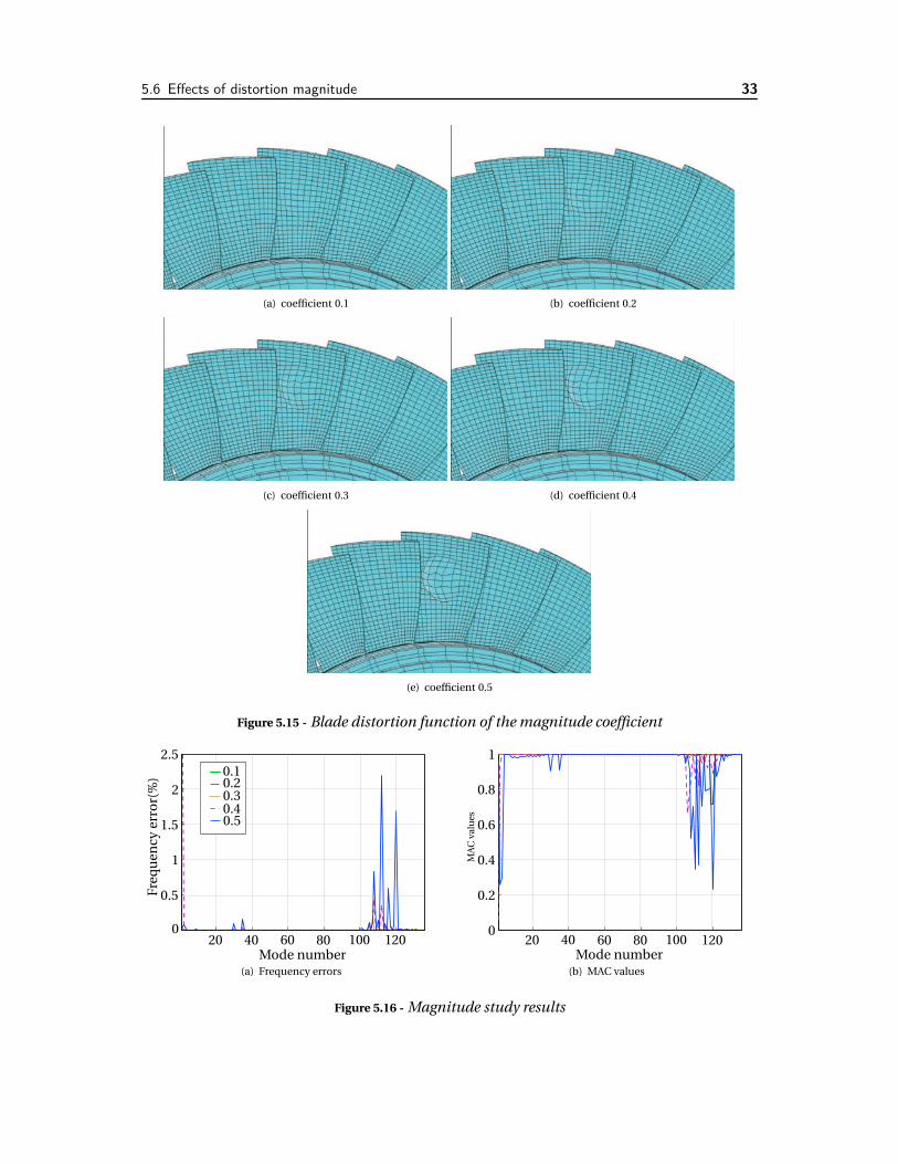
5.6 Effects of distortion magnitude 33

(a) coefficient 0.1 (b) coefficient 0.2

(c) coefficient 0.3 (d) coefficient 0.4

(e) coefficient 0.5

Figure 5.15 - Blade distortion function of the magnitude coefficient

Mode number

Freq

uen

cyer

ror(

%) 0.1

0.20.30.40.5

20 40 60 80 100 1200

0.5

1

1.5

2

2.5


Mode number

MA

Cva

lues

20 40 60 80 100 1200

0.2

0.4

0.6

0.8

1

(b) MAC values

Figure 5.16 - Magnitude study results

34 Large mistuning

• even a very localized perturbation to several DOFs can have a dramatic effect on the

perturbed system eigenpairs, creating harder modes to approximate.

• the scaling of geometry shape (selected for convenience) is not proportional to the am-

plitude of perturbation, defined by ‖M−1K‖.

6Forced response analysis

combining large and smallmistunings

In this chapter, QSMC and CMM techniques are used to compute the dynamic response of

a geometrically mistuned bladed disk featuring also small parameters variations. This is the

same disk used in the last chapter, in the section where the convergence of a bladed disk con-

taining different patterns of mistuning has been proved (see figure 5.8). But in this case, the

different colors of every blades have a signification: underline the presence of small mistun-

ing, introduced on the nominal Young’s modulus as:

En = E0(1+δen) (6.1)

where En is the new Young’s modulus of the n th blade, E0 is the original nominal Young’s

modulus and δen

is a non-dimensional mistuning value. The specific pattern used in this

case is shown in table 6.1. Although the proportional blade to blade stiffness variation intro-

duced by changing Young’s modulus of the blades is a very rough way to model random small

mistuning phenomena, it has been chosen for simplicity to validate the accuracy of the de-

velopped method. In this study the structural damping coefficient is set to 0.006, the modal

participation factors are calculated using 30 cantilevered-blade modes, with only a third of

them dominant.

Blade n 1 2 3 4 5 6 7 8 9 10

δen

5.704 1.207 4.67 -1.502 5.969 -3.324 -0.078 -1.688 0.242 -2.747

Blade n 11 12 13 14 15 16 17 18 19 20

δen

-3.631 -3.57 -6.31 -3.631 0.242 4.934 4.479 3.03 0.242 1.734

Blade n 21 22 23 24 25 26 27 28 29

δen

2.919 -0.328 0.086 -3.654 -3.631 -1.665 0.783 -1.169 -1.332

Table 6.1 - Eigenvalue mistuning pattern

36 Forced response analysis combining large and small mistunings

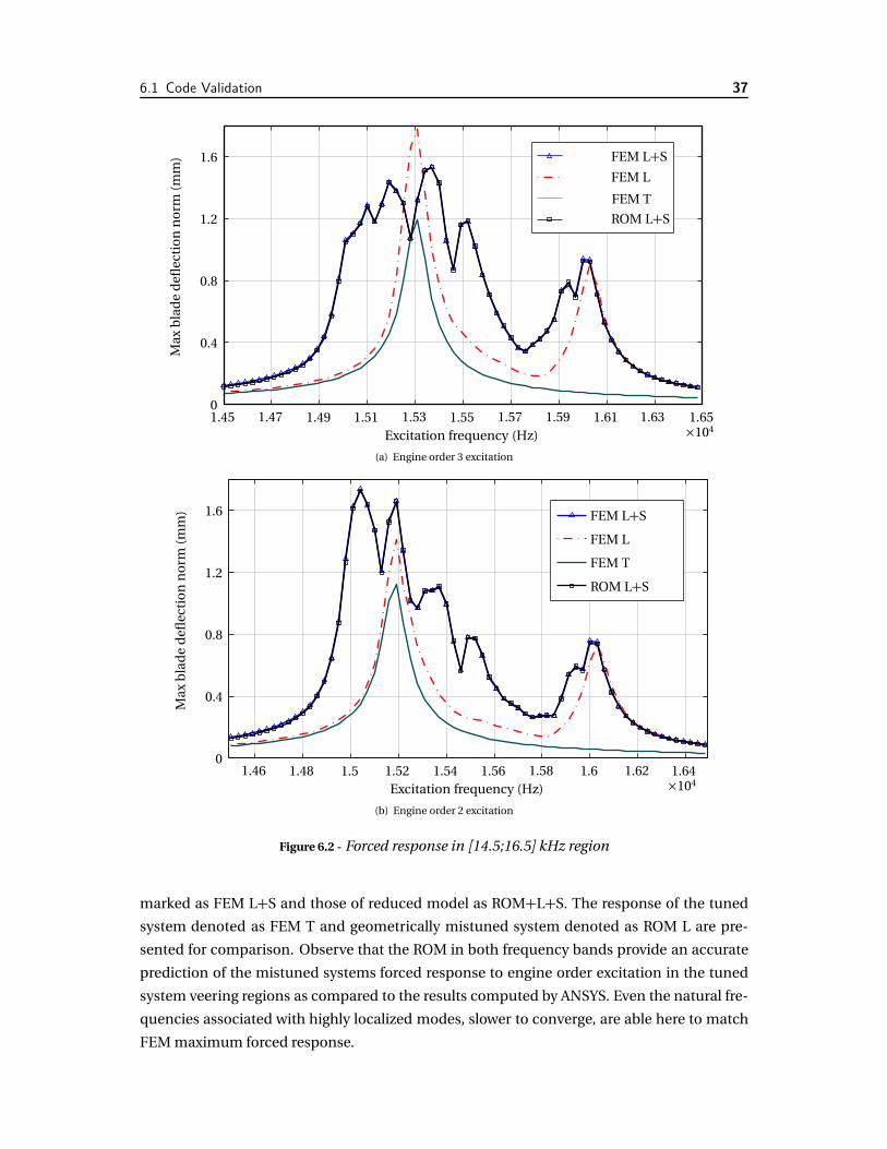
6.1 Code Validation

Despite the large changes in geometry the aerodynamics mistuning is neglected; the forc-

ing function applied corresponds to the 3 and 5 nodal diameter excitation for a 71 tuned-

modes projection ROM, in the [30;37] kHz region, and 2 and 3 engine order (EO) excitation

for a 71 tuned-modes projection ROM in the [14.6;16.6] kHz region. An arbitrary load is ap-

plied at a tip of each blade.

Figure 6.1 shows the euclidiean displacement norms for maximum responding blade ver-

sus frequency of excitation from 33 kHz to 36 kHz, for EO 5 and EO 3 respectively. The results

for [14.5;16.5] kHz region for EO 3 and EO2 are depicted in figure 6.2. ANSYS results are

Excitation frequency (Hz)

Max

bla

de

defl

ecti

on

no

rm(m

m)

FEM L+S

FEM L

FEM T

ROM L+S

3.3 3.35 3.4 3.45 3.5 3.55 3.6×104

0

0.4

0.8

1.2

(a) Engine order 5 excitation


Max

bla

de

defl

ecti

on

no

rm(m

m)

FEM L+S

FEM L

FEM T

ROM L+S

3.3 3.35 3.4 3.45 3.5 3.55 3.6×104

0

0.4

0.8

1.2

(b) Engine order 3 excitation

Figure 6.1 - Forced response in [33;36] kHz region

6.1 Code Validation 37


Max

bla

de

defl

ecti

on

no

rm(m

m) FEM L+S

FEM L

FEM T

ROM L+S

1.45 1.47 1.49 1.51 1.53 1.55 1.57 1.59 1.61 1.63 1.65×104

0

0.4

0.8

1.2

1.6

(a) Engine order 3 excitation


Max

bla

de

defl

ecti

on

no

rm(m

m) FEM L+S

FEM L

FEM T

ROM L+S

1.46 1.48 1.5 1.52 1.54 1.56 1.58 1.6 1.62 1.64×104

0

0.4

0.8

1.2

1.6

(b) Engine order 2 excitation

Figure 6.2 - Forced response in [14.5;16.5] kHz region

marked as FEM L+S and those of reduced model as ROM+L+S. The response of the tuned

system denoted as FEM T and geometrically mistuned system denoted as ROM L are pre-

sented for comparison. Observe that the ROM in both frequency bands provide an accurate

prediction of the mistuned systems forced response to engine order excitation in the tuned

system veering regions as compared to the results computed by ANSYS. Even the natural fre-

quencies associated with highly localized modes, slower to converge, are able here to match

FEM maximum forced response.


Note that the introduction of large mistuning in the studied disk generate the presence of

additional resonance peaks in both frequency band, and for the different EOs. Furthermore, if

we take the example of the frequency region [33;36] kHz, we can see that the additional peaks

are situated at frequencies associated with rogue-blade dominated modes of the mistuned

disk. Thus, the figure 6.1 shows that ROM has accurately predicted those problematic modes.

6.2 Monte-Carlo analysis

The goal of this study is two-fold:

1. Validation of the developed code and demonstration of its computational power, as-

sessment of time necessary for a given size problem.

2. Assessment of sensitivity of the selected geometrical mistuning to the additional small

random mistuning.

Validation 1

The simulation consists of a frequency sweep between 33 KHz and 36 KHz with 10 Hz

step for 100 different mistuning patterns obtained from Gaussian distribution; different small

mistuning levels (spanning from 1% to 15 %) are applied to both geometrically mistuned sys-

tem and a perfectly tuned system. Forced response amplitudes of the mistuned system were

normalized with respect to maximum amplitudes of the tuned bladed disc under the same

excitation conditions. The damping loss factor was set to 0.006. Subsequently, a statistical

analysis is carried out to obtain the probability density and cumulative density functions of

the forced response for maximum values (determined with Weibull PDF fit that, see ?, repre-

sents the best match to the empirical distributions of forced responses obtained from the MC

simulations).

The 99th percentile of the maximum blade response amplitude under all engine order ex-

citations for geometrically mistuned system and tuned system respectively are depicted in

figures 6.3 and 6.4. From the results it is evident that the normalized forced response ulti-

mately decreases as the small mistuning level is increased, and dramatically varies depending

on the engine order of excitation, with maximum at EO 1 for both cases.

The effect of the addition of geometrical mistuning as a difference between the two test

case results is presented in figure 6.5, with some selected EO excitations presented in fig-

ure 6.6 The results obtained indicate for example a reduction in the maximum forced re-

sponse of approximately 144%, from 0.18 at 1% level of small mistuning to -0.08 at 4% of

small mistuning, for EO 8 excitation.

As we can see there are both positive and negative effects of addition of that geometric

mistuning pattern, for EO 1, EO2, EO 8 there is the tendency of the forced response ampli-

fication factor to decrease and the contrary tendency is observed for EO 12 and EO 0. The

rest of nodal diameter excitation does not exhibit any noticeable change in forced response

amplification factor for a given geometrical mistuning pattern.

6.2 Monte-Carlo analysis 39

14 13 12 11 10 9 8 7 6 5 4 3 2 1 0

0

5

10

15

1

1.5

2

2.5

3

Engine Order Excitaion

Mistuning, %

99

−th

Pe

rce

nti

le A

mp

li"

cati

on

Figure 6.3 - Small Mistuning Sensitivity Analysis on Geometrically Mistuned Disk for [33;36] kHz

14 13 12 11 10 9 8 7 6 5 4 3 2 1 0

0

5

10

15

1

1.5

2

2.5

3

Engine Order Excitation

Mistuning, %

99

−th

Pe

rce

nti

le A

mp

li"

cati

on

Figure 6.4 - Small Mistuning Sensitivity Analysis for [33;36] kHz

Validation 2

Overall the 71 DOF ROM was solved 6750000 times, it took 4 hours on Intel XEON Quad

core 2.6 GHz platform with 4G memory, which demonstrates an acceptable computational


14131211109876543210

2

4

6

8

10

−0.05

0

0.05

0.1

0.15

0.2

0.25

Small Mistuning, %

Di!erence, 33−36 KHz

Engine Order Excitation

99

−th

Pe

rce

nti

le A

mp

li"

cati

on

Figure 6.5 - Differences between the two test case results

1 2 3 4 5 6 7 8 9 10 11−0.1

−0.05

0

0.05

0.1

0.15

0.2

0.25

0.3

Small Mistuning,

99−t

h Pe

rcen

tile

Ampl

i!ca

tio

n

EO 12

EO 2

EO 0

EO 8

EO 1

Figure 6.6 - Difference for Selected EOs

time for practical experiments, with industrial size FEM designs.

7Conclusion

A general reduced-order modeling framework was developed by combining CMM and QSMC

methods to analyze geometrically mistuned disks undergoing small random mechanical vari-

ations.

Starting with a finite element model of an industrial turbomachinery rotor, the general

ROM was validated for large mistuning cases, in which one or several blade(s) was (were)

damaged and featured one or several significant geometric change(s) from the tuned de-

sign. It was observed that the estimated natural frequencies of the mistuned rotor converged

rapidly as the selected number of tuned-system modes was increased. Moreover, a study was

carried out in order to suggest how to select those additional tuned-modes in a more eco-

nomic way.

Also, the forced response results from the ROM showed excellent agreement with the FEM

results, and Monte-Carlo simulations have demonstrated that stochastic analysis can be re-

alized in a fast and efficient way, and that provides practical results for sensitivity to small

random mistuning study of geometrical mistuned bladed disks.

An interesting future work would be to optimize tuned-modes selection modes, in order

to anticipate the mistuned structure behavior without having convergence studies to realize.

42 Conclusion

AQuasi-static terms computation

module

This appendix presents the test-case used to make the comparison between MKL-DSS and

Pardiso, in order to present an insight of the MKL-DSS structure. Input matrices of a single

sector are retrieved from text files, and then the inversion giving the quasi-static modes is

computed.

program Calculate_Ansys_Bin

use mkl_dss

implicit none

real(8) :: CenterFreq, val

real(8), allocatable :: TempM(:,:), TempK(:,:), Psi(:,:),&

PsiMPsi(:,:), Temp(:,:), V(:,:), Mmao(:), Smao(:)

integer :: i, j, l, MaxDia, SectorDOFs, Harm, &

Sector_Nodes, MistdoFs, Blade_DOFs

real(8) :: x, t1, t2

integer, pointer :: Mmiao(:), Mmjao(:), Smiao(:), Smjao(:), perm(:)

integer :: k0, iad, i1, nnzK, nnzM, err1, nnz

integer :: ierr, lenS, lenSj

integer, parameter :: bufLen = 20

type(MKL_DSS_HANDLE) :: handle !allocate storage for the solver handle

real(8),allocatable :: statOUt( : )

character(15) :: statIn

44 Quasi-static terms computation module

integer :: buff(bufLen), Inter

integer, pointer :: indu(:)=> null(), iwk(:)=> null()

integer :: ii,jj,kk,count,

Allocation_Status = 0

real(8), parameter :: PI=3.1415926535897932384626433832795d0

integer(8) :: pt(64)

integer :: maxfct, mnum, mtype, phase, msglvl

integer(8) :: iparm(64)

integer :: idum

real(8) :: ddum

integer :: omp_get_max_threads

external :: omp_get_max_threads

data maxfct /1/, mnum /1/

Blade_DOFs = 832*3

CenterFreq = 33000.0d0

perm = 0

!========= Linear System Solver Mistuned DOFs Vector Allocation ==========

V = 0.0d0

j = 0

! read V from a text file

open(1,file=’Fold\V.txt’)

read (1,*) Sectordofs, MistdoFs

allocate(V(Sectordofs, MistdoFs))

do while (.NOT.EOF(1))

read (1,*) ii,jj, V(ii,jj)

end do

close(1)

! read M

open(2,file=’Fold\Mparsevalj.txt’)

read (2,*) nnzM

allocate (Mmao(nnzM))

allocate (Mmjao(nnzM))


read (2,*) ii,Mmao(ii), Mmjao(ii)

end do

close(2)

45

allocate (Mmiao(SectorDOFs+1))

open(3,file=’Fold\Mparsei.txt’)


read (3,*) ii,Mmiao(ii)

end do

close(3)

! read St

open(4,file=’Fold\Sparsevalj.txt’)

read (4,*) nnz

allocate (Smao(nnz))

allocate (Smjao(nnz))


read (4,*) ii,Smao(ii), Smjao(ii)

end do

close(4)

allocate (Smiao(SectorDOFs+1))

open(5,file=’Fold\Sparsei.txt’)


read (5,*) ii,Smiao(ii)

end do

close(5)

!======================= DSS Solver ====================================

! Initialize the DSS solver.

allocation_status=0

allocate(Psi(SectorDOFS,MistDOFs),stat=allocation_status)

if (Allocation_Status /=0) write(*,*) ’Harmonic mass allocation failed’

Psi=0.0d0

call cpu_time(t1)

write(*,*)’ DSS tic ’

err1=DSS_CREATE(handle, MKL_DSS_DEFAULTS)

if (err1/=MKL_DSS_SUCCESS) write(*,*)’DSS solver failed, error =’,err1

! Define the non-zero structure of the matrix.

err1=DSS_DEFINE_STRUCTURE(handle,MKL_DSS_SYMMETRIC,Smiao(1:nnz),SectorDOFs,

SectorDOFs,Smjao(1:nnz),nnz)

if (err1/=MKL_DSS_SUCCESS) write(*,*)’DSS solver failed, error = ’,err1


! Reorder the matrix.

err1=DSS_REORDER( handle, MKL_DSS_DEFAULTS, perm )


! Factor the matrix

err1=DSS_FACTOR_REAL(handle,MKL_DSS_INDEFINITE,Smao(1:nnz))


err1=DSS_SOLVE_REAL(handle,MKL_DSS_DEFAULTS,V,MistDOFs,Psi)


! Print Out the determinant of the matrix

if (SectorDOFs.LT.nnz-1) then

allocate(statOut( 5 ))

statIn=’determinant’

call mkl_cvt_to_null_terminated_str(buff,bufLen,statIn)

err1=DSS_STATISTICS(handle, MKL_DSS_DEFAULTS, buff, statOut)


write(*,"(’pow of determinant is ’(5F10.3))") (statOut(1))

write(*,"(’base of determinant is ’(5F10.3))") (statOut(2))

write(*,"(’Determinant is ’(E24.18))") (real((10**statOut(1))*statOut(2), 16))

deallocate(statOut)

end if

! Deallocate solver storage and various local arrays

err1=DSS_DELETE(handle,MKL_DSS_DEFAULTS)


!============== end of DSS solver ===========================================

write(*,*)’ DSS toc ’

call cpu_time(t2)

write(*,*)’ Time taken by DSS ’, t2-t1, ’seconds’

allocate(PsiMPsi(MistDOFs,MistDOFs))

allocate(tempM(SectorDOFs,MistDOFs))

call cpu_time(t1)

write(*,*)’ DSS tic ’

call mkl_dcsrmm(’N’,SectorDOFs,MistDOFs,SectorDOFs,1.0d0,’SUN’,Mmao,Mmjao,

47

Mmiao,Mmiao(2),Psi,SectorDOFs,0.0d0,tempM,SectorDOFs)

call dgemm(’T’,’N’,MistDOFs,MistDOFs,SectorDOFs,1.0d0,Psi,SectorDOFs,tempM,

SectorDOFs,0.0d0,PsiMPsi,MistDOFs)

write(*,*)’ DSS toc ’

call cpu_time(t2)

write(*,*)’ Time taken by PsiMPsi multiplication ’, t2-t1, ’seconds’

deallocate(tempM)

deallocate(Mmao,Mmiao,Mmjao,Smao,Smiao,Smjao,V)

end program Calculate_Ansys_Bin


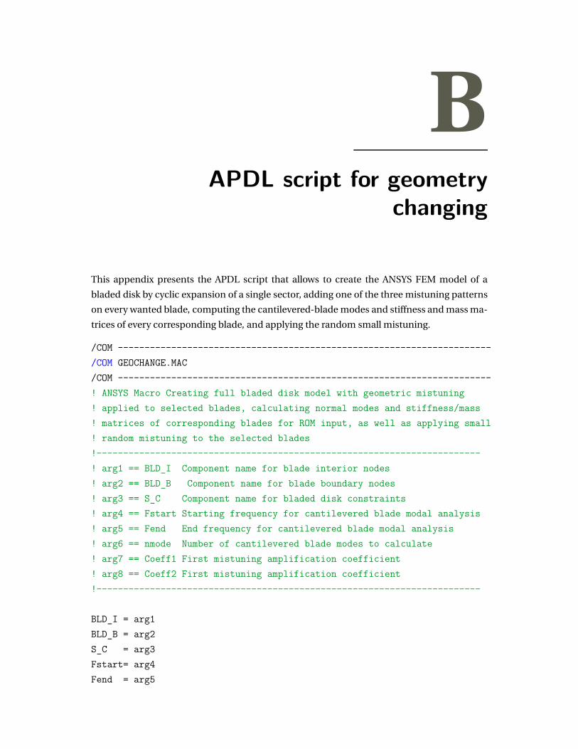
BAPDL script for geometry

changing

This appendix presents the APDL script that allows to create the ANSYS FEM model of a

bladed disk by cyclic expansion of a single sector, adding one of the three mistuning patterns

on every wanted blade, computing the cantilevered-blade modes and stiffness and mass ma-

trices of every corresponding blade, and applying the random small mistuning.

/COM ----------------------------------------------------------------------

/COM GEOCHANGE.MAC

/COM ----------------------------------------------------------------------

! ANSYS Macro Creating full bladed disk model with geometric mistuning

! applied to selected blades, calculating normal modes and stiffness/mass

! matrices of corresponding blades for ROM input, as well as applying small

! random mistuning to the selected blades

!------------------------------------------------------------------------

! arg1 == BLD_I Component name for blade interior nodes

! arg2 == BLD_B Component name for blade boundary nodes

! arg3 == S_C Component name for bladed disk constraints

! arg4 == Fstart Starting frequency for cantilevered blade modal analysis

! arg5 == Fend End frequency for cantilevered blade modal analysis

! arg6 == nmode Number of cantilevered blade modes to calculate

! arg7 == Coeff1 First mistuning amplification coefficient

! arg8 == Coeff2 First mistuning amplification coefficient

!------------------------------------------------------------------------

BLD_I = arg1

BLD_B = arg2

S_C = arg3

Fstart= arg4

Fend = arg5

50 APDL script for geometry changing

nmode = arg6

Coeff1= arg7

Coeff2= arg8

alpha = 12.4137931

ns=nint(360./alpha)

*dim,mist,array,ns

!rogue blade distribution within the bladed disk, starting with

!blade 2 up to 1 through the last one

mist(1) = 0,1,0,0,0,0,0,0,0,0

mist(11)= 0,0,0,2,0,0,0,0,3,0

mist(21)= 0,0,0,1,0,0,0,0,0

!small proportional mistuning Young’s modulus variations

*dim,deltaYoung,array,ns

deltaYoung(1) = 0.05704



deltaYoung(4) = -0.01502






deltaYoung(10)= -0.02747





deltaYoung(15)= 0.00242











51





!small proportional mistuning density variations

*dim,deltaDens,array,ns

deltaDens(1) = 0.00704



deltaDens(4) = -0.00502


deltaDens(6) = -0.00323

deltaDens(7) = -0.00078

deltaDens(8) = -0.00688


deltaDens(10)= -0.00747

deltaDens(11)= -0.00631

deltaDens(12)= -0.00570

deltaDens(13)= -0.00631

deltaDens(14)= -0.00631

deltaDens(15)= 0.00242







deltaDens(22)= -0.00328


deltaDens(24)= -0.00654

deltaDens(25)= -0.00631

deltaDens(26)= -0.00665


deltaDens(28)= -0.00169

deltaDens(29)= -0.00332

! traveling wave excitation vector

!============================================

freq1 = 26000.0


freq2 = 43000.0

strDamping = 0.006

EO = 5.0

nnodesF = 1

! how many nodes to force

*dim,Forcing,,nnodesF,3

*dim,ForcingNodeIDs,,nnodesF

ForcingNodeIDs(1)=1680

Forcing(1,1)=-51.2440

Forcing(1,2)=22.9220

Forcing(1,3)=-13.0584

!=============================================

/prep7

cmsel,S,%BLD_B%

cmsel,A,%BLD_I%

*get,bladeNodeStart,node,,num,min

*get,bladeNodeEnd,node,,num,max

allsel

*get,ntot,node,,num,max

*get,etot,elem,,num,max

! Get the sector constrained node numbers array

cmsel,S,%S_C%

*get,mxnd,node,,num,max ! Get the max node number

*dim,nds,,mxnd ! Make the node array

*dim,nmsk,,mxnd ! Make the node mask array

*vfill,nds(1),ramp,1,1 ! Fill nds first column with node numbers

*vget,nmsk(1),node,1,nsel ! Figure out what is selected: creates mask

*vmask,nmsk(1) ! Mask on selected nodes

*vscfun,num_nd,NUM,nmsk(1) ! Count the total number of selected nodes

*dim,constr,,num_nd ! Make the node - dof mapping array

53


*vfun,constr(1),COMP,nds(1) ! Selectively compresses data set. "True" values of nds

*get,numnd,PARM,constr,DIM,X

!Get the blade interface constrained node numbers array

cmsel,S,%BLD_B%

*get,mxnd,node,,num,max ! Get the max node number

*dim,nds,,mxnd ! Make the node array

*dim,nmsk,,mxnd ! Make the node mask array

*vfill,nds(1),ramp,1,1 ! Fill nds first column with node numbers

*vget,nmsk(1),node,1,nsel ! Figure out what is selected: creates mask


*vscfun,num_nd,NUM,nmsk(1) ! Count the total number of selected nodes

*dim,inconstr,,num_nd ! Make the node - dof mapping array


*vfun,inconstr(1),COMP,nds(1) ! Selectively compresses data set. "True" values of nds

*get,innumnd,PARM,inconstr,DIM,X

! Arrays definition for the first pattern

*dim,arraymodif1,array,70,4

*VREAD,arraymodif1(1,1),Nodemodif1,txt,,jik,4,70,,

(F8.0,E13.5,2E12.5)

*dim,InitialNodes1,array,70,3

*do,ii,1,70

*vget,InitialNodes1(ii,1),node,ArrayModif1(ii,1),loc,x

*vget,InitialNodes1(ii,2),node,ArrayModif1(ii,1),loc,y

*vget,InitialNodes1(ii,3),node,ArrayModif1(ii,1),loc,z

*enddo

! Arrays definition for the second pattern

*dim,arraymodif2,array,93,4

*VREAD,arraymodif2(1,1),Nodemodif2,txt,,jik,4,93,,

(F8.0,E13.5,2E12.5)


*dim,InitialNodes2,array,93,3

*do,ii,1,93

*vget,InitialNodes2(ii,1),node,ArrayModif2(ii,1),loc,x

*vget,InitialNodes2(ii,2),node,ArrayModif2(ii,1),loc,y

*vget,InitialNodes2(ii,3),node,ArrayModif2(ii,1),loc,z

*enddo

*do,ii,1,ns

*if,ii,NE,ns,then

chst = chrval(ii+1)

*else

chst = chrval(1)

*endif

mfil = ’RogueBlade_%chst%’

*if,mist(ii),EQ,1,then

/assign,full,RogueBlade_%chst%,full

/assign,mode,RogueBlade_%chst%,mode

/prep7

csys,0

nsel,s,node,,1,ntot

*do,jj,1,70

NMODIF,ArrayModif1(jj,1),InitialNodes1(jj,1)+Coeff1*ArrayModif1(jj,2),

InitialNodes1(jj,2)+Coeff1*ArrayModif1(jj,3),

InitialNodes1(jj,3)+Coeff1*ArrayModif1(jj,4),0,0,0

*enddo

*finish

*msg,,

--- Done with modifyning current rogue blade -------------------

/go

/solu

cmsel,S,%BLD_B%

cmsel,A,%BLD_I%

esln,S,1

antype,2

55

msave,0

modopt,LANB,5

eqslv,SPAR

mxpand,5, , ,0

lumpm,0

pstres,0

modopt,LANB,5,1000,50000, ,OFF

solve

*finish

/assign,FULL,,

*msg,,

--- Done with extracting mass and stiffness matrices

/go

/prep7

!impose constraints to the blade interface nodes

*do,ndnum,1,innumnd

d,inconstr(ndnum),all,0.0,,,,,,,

*enddo

!d,865,all,0,,896,1,,,,

*finish

/solu

antype,2

msave,0

modopt,LANB,nmode

eqslv,SPAR

mxpand,nmode, , ,0

lumpm,0

pstres,0

modopt,LANB,nmode,Fstart,Fend, ,OFF

/solu

solve

*finish

! delete constraints to the interface

/assign,MODE,,

/prep7

*do,ndnum,1,innumnd

ddele,inconstr(ndnum),all

*enddo

!ddele,865,all,896,1,

*finish


*msg,,

--- Done with extracting modes

/go

*elseif,mist(ii),EQ,2,then



/prep7

csys,0

nsel,s,node,,1,ntot

*do,jj,1,93

NMODIF,ArrayModif2(jj,1),InitialNodes2(jj,1)+Coeff2*ArrayModif2(jj,2),

InitialNodes2(jj,2)+Coeff2*ArrayModif2(jj,3),InitialNodes2(jj,3)

+Coeff2*ArrayModif2(jj,4),0,0,0

*enddo

*finish

*msg,,


/go

/solu

cmsel,S,%BLD_B%

cmsel,A,%BLD_I%

esln,S,1

antype,2

msave,0

modopt,LANB,5

eqslv,SPAR

mxpand,5, , ,0

lumpm,0

pstres,0


solve

*finish

/assign,FULL,,

*msg,,


/go

/prep7


*do,ndnum,1,innumnd

57


*enddo

!d,865,all,0,,896,1,,,,

*finish

/solu

antype,2

msave,0

modopt,LANB,nmode

eqslv,SPAR

mxpand,nmode, , ,0

lumpm,0

pstres,0


/solu

solve

*finish


/assign,MODE,,

/prep7

*do,ndnum,1,innumnd


*enddo

!ddele,865,all,896,1,

*finish

*msg,,


/go

*elseif,mist(ii),EQ,3,then



/prep7

csys,0

nsel,s,node,,1,ntot

scale = rand(1,1.1)

first = 1!1.2*scale

second = 1!1.16*scale

third = 1!1.11*scale

fourth = 1!1.05*scale


fifth = 1!1.0*scale

!first round

*finish

*msg,,


/go

/solu

cmsel,S,%BLD_B%

cmsel,A,%BLD_I%

esln,S,1

antype,2

msave,0

modopt,LANB,5

eqslv,SPAR

mxpand,5, , ,0

lumpm,0

pstres,0


solve

*finish

/assign,FULL,,

*msg,,


/go

/prep7


*do,ndnum,1,innumnd


*enddo

!d,865,all,0,,896,1,,,,

*finish

/solu

antype,2

msave,0

modopt,LANB,nmode

eqslv,SPAR

mxpand,nmode, , ,0

lumpm,0

pstres,0


59

/solu

solve

*finish


/assign,MODE,,

/prep7

*do,ndnum,1,innumnd


*enddo

!ddele,865,all,896,1,

*finish

*msg,,


/go

*endif

*if,ii,NE,1,AND,mist(ii),EQ,0,then

*if,mist(ii-1),EQ,1,then

/prep7

csys,0

nsel,s,node,,1,ntot

*do,jj,1,70

NMODIF,ArrayModif1(jj,1),InitialNodes1(jj,1),InitialNodes1(jj,2),

InitialNodes1(jj,3),0,0,0

*enddo

*finish

*msg,,

----- Done with returning to tuned blade -----

/go

*elseif,mist(ii-1),EQ,2,then

/prep7

csys,0

nsel,s,node,,1,ntot

*do,jj,1,93

NMODIF,ArrayModif2(jj,1),InitialNodes2(jj,1),InitialNodes2(jj,2),

InitialNodes2(jj,3),0,0,0

*enddo

*finish

*msg,,



/go

*elseif,mist(ii-1),EQ,3,then

/prep7

csys,0

nsel,s,node,,1,ntot

*finish

*msg,,


/go

*endif

*endif

*if,ii,NE,ns,then

/prep7

cmsel,S,%BLD_B%

cmsel,A,%BLD_I%

esln,S,1

! create current blade’s material properties for proportional small mistuning

mptemp,,,,,,,,

mptemp,1,0

uimp,ii+2,REFT,,,70

mpde,EX,ii+2

mpde,NUXY,ii+2

mpde,DENS,ii+2

mpde,ALPX,ii+2

mpdata,DENS,ii+2,,0.00074014*(1+deltaDens(ii+1))

mpdata,EX,ii+2,,29500000*(1+deltaYoung(ii+1))

mpdata,NUXY,ii+2,,0.305

mpdata,ALPX,ii+2,,5.16E-006

! modify current blade’s material properties for proportional small mistuning

emodif,ALL,MAT,ii+2

nsel,s,node,,1,ntot

esel,s,elem,,1,etot

csys,11

! generate nodes ns times incrementing nodes by ntot each time

! from node 1 to node ntot incrementing by 1 with node

! location increments in the active coordinate system DY=alpha

ngen,2,ntot*ii,1,ntot,1,,alpha*ii

61

egen,2,ntot*ii,1,etot,

! replicate constraints

*do,ndnum,1,numnd

d,constr(ndnum)+ntot*ii,all,0.0,,,,,,,

*enddo

! apply travelling wave forcing excitation

*do,ndnum,1,nnodesF

f,ForcingNodeIDs(ndnum)+ntot*ii,FX,(cos(alpha*(ii)*EO)*Forcing(ndnum,1)),(sin(alpha*(ii)*EO)*Forcing(ndnum,1))

f,ForcingNodeIDs(ndnum)+ntot*ii,FY,(cos(alpha*(ii)*EO)*Forcing(ndnum,2)),(sin(alpha*(ii)*EO)*Forcing(ndnum,2))

f,ForcingNodeIDs(ndnum)+ntot*ii,FZ,(cos(alpha*(ii)*EO)*Forcing(ndnum,3)),(sin(alpha*(ii)*EO)*Forcing(ndnum,3))

*enddo

! generate current blade component to calculate blade’s Eucleadean norm

nsel,s,node,,bladeNodeStart+ntot*ii,bladeNodeEnd+ntot*ii

cm,Blade_%chst%,node

! return back the material properties of the initial blade

cmsel,S,%BLD_B%

cmsel,A,%BLD_I%

esln,S,1

emodif,ALL,MAT,1

*finish

*else

! first blade material modification

/prep7

mptemp,,,,,,,,

mptemp,1,0

uimp,2,REFT,,,70

mpde,EX,2

mpde,NUXY,2

mpde,DENS,2

mpde,ALPX,2

mpdata,DENS,2,,0.00074014*(1+deltaDens(1))

mpdata,EX,2,,29500000*(1+deltaYoung(1))

mpdata,NUXY,2,,0.305

mpdata,ALPX,2,,5.16E-006

cmsel,S,%BLD_B%

cmsel,A,%BLD_I%

esln,S,1

emodif,ALL,MAT,2

! apply travelling wave forcing excitation to the first blade


*do,ndnum,1,nnodesF

f,ForcingNodeIDs(ndnum),FX,(cos(alpha*(0)*EO)*Forcing(ndnum,1)),(sin(alpha*(0)*EO)*Forcing(ndnum,1))

f,ForcingNodeIDs(ndnum),FY,(cos(alpha*(0)*EO)*Forcing(ndnum,2)),(sin(alpha*(0)*EO)*Forcing(ndnum,2))

f,ForcingNodeIDs(ndnum),FZ,(cos(alpha*(0)*EO)*Forcing(ndnum,3)),(sin(alpha*(0)*EO)*Forcing(ndnum,3))

*enddo

! generate current blade component to calculate blade’s Eucleadean norm

nsel,s,node,,bladeNodeStart,bladeNodeEnd

cm,Blade_%chst%,node

*finish

*endif

*enddo

/prep7

allsel csys,11 nrotat,all ! merge nodes

nummrg,node,1.0e-03,,,high

allsel csys,0 nrotat,all

*finish

!------------------------------------------------------------------------

! Clear parameters

mfil =

BLD_I =

BLD_B =

S_C =

Fstart =

Fend =

nmode =

constr =

alpha =

mist =

scale =

first =

second =

third =

fourth =

fifth =

numnd =

innumnd =

deltaDens =

deltaYoung =

63

EO =

nnodesF =

ForcingNodeIDs =

Forcing =

Documents

Reduced Order Modeling of Bladed Disks Featuring Large ...structdynviblab.mcgill.ca/pdf/TFEVarin.pdf · Reduced Order Modeling of Bladed Disks Featuring Large Mistuning ... late the