Redox entropy of plastocyanin: Developing a microscopic

Redox entropy of plastocyanin: Developing a microscopic viewof mesoscopic polar solvation

David N. LeBard and Dmitry V. Matyushova�

Center for Biological Physics, Arizona State University, PO Box 871604, Tempe, Arizona 85287-1604, USA

�Received 2 November 2007; accepted 12 March 2008; published online 18 April 2008�

We report applications of analytical formalisms and molecular dynamics �MD� simulations to thecalculation of redox entropy of plastocyanin metalloprotein in aqueous solution. The goal of ouranalysis is to establish critical components of the theory required to describe polar solvation at themesoscopic scale. The analytical techniques include a microscopic formalism based on structurefactors of the solvent dipolar orientations and density and continuum dielectric theories. Themicroscopic theory employs the atomistic structure of the protein with force-field atomic chargesand solvent structure factors obtained from separate MD simulations of the homogeneous solvent.The MD simulations provide linear response solvation free energies and reorganization energies ofelectron transfer in the temperature range of 280–310 K. We found that continuum modelsuniversally underestimate solvation entropies, and a more favorable agreement is reported betweenthe microscopic calculations and MD simulations. The analysis of simulations also suggests thatdifficulties of extending standard formalisms to protein solvation are related to the inhomogeneousstructure of the solvation shell at the protein-water interface combining islands of highly structuredwater around ionized residues along with partial dewetting of hydrophobic patches. Quantitativetheories of electrostatic protein hydration need to incorporate realistic density profile of water at theprotein-water interface. © 2008 American Institute of Physics. �DOI: 10.1063/1.2904879�

I. INTRODUCTION

Calculations of the thermodynamics of hydratedbiopolymers present a significant challenge to theoretical al-gorithms. In many cases the problem can be treated by nu-merical simulations with force fields assigned to the biomol-ecule �solute� and water �solvent�.1 The obvious difficulty isthe large computational load and still existing uncertaintiesin the treatment of the long-range electrostatics. The prob-lem, however, becomes more nontrivial when derivatives ofthermodynamic potentials, e.g., redox entropy, need to becomputed or when the solvation thermodynamics changes onthe time and length scale unattainable to standard moleculardynamics �MD� protocols, e.g., in problems related to pro-tein folding.2,3 In all such cases, coarse graining of the sys-tem is required and that can be done on various lengthscales.4–6 Dielectric continuum algorithms, solving theboundary Poisson problem, are computationally very effi-cient. In this approximation, all length scales below the larg-est distance of microscopic correlations �density and/or po-larization� are averaged out into a continuum surrounding thesolute. These approaches are normally represented by eitherdirect solution of the Poisson–Boltzmann equation on thereal-space grid7 or even more approximate formalisms underthe umbrella of the generalized Born approximation.8

When the cavity cut out by the solute from the con-tinuum dielectric is properly parametrized, equations of con-tinuum electrostatics provide a reasonable estimate of thesolvation Gibbs energy.9–11 The fundamental problem of this

approach is that the local structure of the solvent around thesolute, averaged out in the continuum limit, is what effec-tively forms the dielectric cavity. While this structure can beparametrized by choosing proper van der Waals �vdW�radii,12 this parametrization needs to be redone every timethe thermodynamic state of the solvent changes. This diffi-culty makes continuum formalisms unreliable for the calcu-lation of derivatives of the Gibbs energy, for instance, theentropy of solvation.13–16 In addition, the surface of a proteinis highly heterogeneous combining hydrophobic patches ex-posing nonpolar residues and hydrophilic patches made ofionized/polar residues. While the water structure is rigidaround ionized residues, probably resembling the well-studied case of solvation around simple ions, water is muchless structured at hydrophobic patches with the potential fordewetting17 or/and oscillations of the water occupation.18,19 Itis clear that simplistic continuum does not represent thiscomplex reality,3 and one needs to incorporate the ability ofthe solvent to fluctuate into the solvation model.

The goal of this paper is to extend the microscopic viewof solvation in polar solvents, which we have been develop-ing in the past in application to small- and medium-sizesolutes,14,15,20 to solvation of solutes of mesoscopic dimen-sion, biopolymers in the first place. The length scale of thisproblem presents an obvious obstacle to numerical simula-tion techniques. On the other hand, the same length scaleallows one to hope that some of the short-range features ofthe solvent structure around the solute, making solvation ofsmall molecules so specific, might average out on a largerscale. If this averaging is realized for solvation of biopoly-mers, it would allow coarse-grained models to efficiently op-a�Electronic mail: [email protected].

THE JOURNAL OF CHEMICAL PHYSICS 128, 155106 �2008�

0021-9606/2008/128�15�/155106/17/$23.00 © 2008 American Institute of Physics128, 155106-1

Downloaded 18 Apr 2008 to 129.219.244.213. Redistribution subject to AIP license or copyright; see http://jcp.aip.org/jcp/copyright.jsp

http://dx.doi.org/10.1063/1.2904879

http://dx.doi.org/10.1063/1.2904879

http://dx.doi.org/10.1063/1.2904879

erate in this field complementing direct numerical simula-tions. Our approach to the problem is to coarse grain thesolvent response into a number of solvent correlation func-tions �structure factors� representing the nuclear modes af-fecting electrostatic solvation. The microscopic nature of thesolvent response is then incorporated into the wave-vectordependence of these structure factors efficiently filtering outthe length scales insignificant for solvation.

This study poses the central question for the future de-velopment of such techniques: What are the solvent modeswhich play the central role in the thermodynamics of meso-scopic polar solvation and what are the theory ingredientscritical for capturing the basic physics of large-scale solva-tion? We study this problem here by carrying out extensiveMD simulations of solvation of plastocyanin �PC� in TIP3Pwater in the temperature range of 280–310 K. This fullyatomistic approach is compared to continuum electrostaticsand to our microscopic algorithm, operating with k-spacecorrelation functions, which was designed to scale efficientlyon the mesoscopic length scale.

Plastocyanin from spinach is a single polypeptide chainof 99 residues forming a �-sandwich, with a single copperion coordinated by two sulfurs from cysteine and methionineand two nitrogens from histidine residues �Fig. 1�. The pres-ence of the copper ion, which can change redox state, allowsPC to function as a mobile electron carrier in the photosyn-thetic apparatus of plants and bacteria. It accepts an electronfrom ferrocytochrome f and diffusionally carries it to anotherdocking location where the electron is donated to the oxi-dized form of photosystem I.21

Because of high solvent accessibility of the redox site,PC presents a convenient model to study the hydration effecton the redox properties of metalloproteins, a situation alsoencountered for ferrodoxins.22,23 The redox thermodynamicsof PC has been characterized experimentally24–26 and com-bined quantum/simulation calculations have been done aswell.27,28 The early focus of the theoretical studies had beenon unusually high redox potentials of copper proteins, whichwas assigned to the nontraditional distorted tetrahedral coor-dination on the copper ion.29–31 In particular, the Cu–S bondto methionine is unusually long and is actually broken in thereduced state of PC at pH�3.8.32 The protein is also highlycharged at pH�7 �−9.0 in reduced state and −8.0 in oxi-dized states�. The charge is made by 15 negatively chargeddeprotonated residues �nine glutamic and six aspartic acids�

and six positively charged lysine residues with amino groupsprotonated �Fig. 2�. The asymmetric charge distribution lo-cated on the protein surface creates the dipole moment of2200 D in the oxidized state �Ox� and of 2470 D in the re-duced state �Red�, both numbers are calculated relative to thecenter of partial charges.

The redox potential of the protein includes a componentfrom the local ligand field of the active site and the Gibbsenergy of solvation. The computation of the former requiresquantum mechanics, making the problem of calculating theoverall redox potential a very nontrivial exercise.23,28,33,34

Calculations of solvation thermodynamics can be reasonablyaccomplished using partial atomic charges parametrizedfrom quantum calculations in the vacuum. The experimentalinput comes from measurements of redox entropy24,25,35

since the temperature-independent ligand-field component isexpected to vanish in the temperature derivative.

II. MICROSCOPIC SOLVATION MODEL

The principal idea of the microscopic solvation model isto reduce the problem of solvation of an arbitrary solute in apolar solvent to a formalism combining two major blocks:Electrostatics of an isolated solute and nonlocal correlationfunctions of the pure solvent. The idea of assembling sepa-rate solute and solvent properties in a solvation model isobviously not new going back to Born36 and Onsager37 andall the subsequent development of continuum electrostaticsin application to solvation.7–10,38 The advantage of our ap-proach is in avoiding the necessity to know the microscopicsolute-solvent structure, which is the main complexity of mi-croscopic solvation models and is also their main advantagewhen the problem is successfully resolved by either solvingintegral equations39 or by applying time-dependent40,41 orequilibrium42–44 density functional methods. Inserting a sol-ute into a dense liquid creates a significant distortion of itsstructure, and the incomplete account of the coupling be-tween the short-range density profile around the solute withthe long-range polarization field is perhaps the weakest partof our formulation when applied to small solutes.45 �Thisdeficiency is almost completely offset by averaging of thedensity profile around a nanoscale solute �see below�.� Onthe other hand, a strong side of our formalism, its ability totreat solvation of large solutes of irregular shape and arbi-trary charge distribution,15,46 becomes particularly useful inapplication to protein solvation.

FIG. 1. �Color� Structure of plastocyanin: the active site includes copper ion�green�, 2 histidines �blue�, methionine �red�, and cysteine �orange� residues.

FIG. 2. �Color� Distribution of the positive and negative charge on thesurface of the protein. The positively and negatively charged residues areshown, respectively, in red and blue. The copper ion is shown in green.

155106-2 D. N. LeBard and D. V. Matyushov J. Chem. Phys. 128, 155106 �2008�


The reduction of the many-body solvation problem to anirreducible representation in terms of a few basic correlationfunctions depends on the symmetry of the solute-solvent in-teraction potential. The number of correlation functions isknown to grow with increasing the rank of the solvent mul-tipole included in the interaction potential.47 Solvent dipolesare for the most part sufficient for solvation in polarliquids,48 in which case the solute-solvent interaction poten-tial V0s �“0” and “s” are used for the solute and solvent,respectively� is a sum of pairwise interactions of the soluteelectric field E0�r� with the solvent dipoles,

V0s = − �j=1

N

m j� · E0�r j� . �1�

Here, m j� is the dipole moment characteristic of the bulk stateof the solvent; m� is usually higher that the vacuum dipole mbecause of the collective field of the induced solventdipoles.49 For instance, the dipole moment of water in theliquid state, 2.4–2.6 D,50 is higher than the gas-phase dipoleof 1.83 D.

We will focus on the electrostatic component of thechemical potential of solvation �0s which contains all theinformation relevant to electrostatic solvation. Linear re-sponse approximation �LRA� significantly simplifies theproblem and provides several equivalent routes to �0s. Onecan consider the full interaction between the atomic chargesof the solute and the solvent and determine �0s as half of theaverage solute-solvent interaction energy,51 �0s= �V0s� /2. Al-ternatively, one can use the second cumulants, ��V0s�2� or��V0s�2�0.14 In the first expression, the angular brackets �…�refer to an ensemble average over the fluctuations �V0s in thesolvent in equilibrium with the full charge distribution of thesolute. For the second expression, �. . .�0 implies that all thecharges of the solute have been set to zero, and fluctuationsof the solvent in the solute vicinity are regulated only byshort-range solute-solvent interactions, molecular repulsionsin the first place. In the LRA, the two cumulants are equal,52

which physically means that the solute electrostatic forces donot significantly change the solvent structure around the sol-ute established by the prevalence of short-range repulsions.53

Computer simulations for the most part support thispicture54–56 with a few exceptions of very strong solute-solvent electrostatic coupling found for small solutes.16,52,57

This observation opens up a significant simplification ofthe calculation algorithms. Instead of solving the inhomoge-neous problem of restructuring the solvent in an externalfield of the solute, it appears to be sufficient to look at thestatistics of solvent fluctuations around the repulsive core ofthe solute. This strategy is used here and we will base ourcalculations on the relation

− �0s = ��/2��V0s�2�0, �2�

where �V0s=V0s− �V0s�0 and �=1 / �kBT�.By using the interaction potential according to Eq. �1�,

one can rewrite Eq. �2� in the form typical for Gaussian�LRA� models of solvation,58,59

− �0s = 12 E0�k1� � ��k1,k2� � E0�k2� . �3�

Here, the two-rank tensor ��k1 ,k2� is the response function60

of the system composed of a dipolar solvent and a solute toa weak field of the solute. The inhomogeneous character ofthe problem is reflected by the fact that ��k1 ,k2� depends ontwo wave vectors, k1 and k2, separately and not on k1−k2, asis the case with response functions of homogeneous solvents.The asterisk in Eq. �3� refers to both the tensor contraction

and integration in inverted k space. In addition, E0�k� is theFourier transform of the electric field of the solute defined bythe integral limited to the solvent volume �

E0�k� = �

E0�r�eik·rdr . �4�

The shape of the solute thus enters both the response func-

tion ��k1 ,k2� and the field Fourier transform E0�k�. Thecharge distribution of the solute, which determines the elec-

tric field E0�k�, is given by its electronic density and is com-monly represented by partial atomic charges.

The main challenge of this formalism, as well as of otherGaussian solvation theories,61 is how to connect the inhomo-geneous response function ��k1 ,k2� to the shape of the sol-ute repulsive core and the self-correlation functions of thesolvent modes affecting solvation. Two modes naturally ap-pear in most theories: Dipolar �orientational� polarizationand density fluctuations.20,43,62,63 For the former, the combi-nation of axial symmetry introduced by the wave vector kwith the vector character of the dipolar polarization P�k�allows one to split the two-rank tensor �s�k�= �� /��P�k�2� into the longitudinal and transverse dyads,64

�s�k� =3y

4��JLSL�k� + JTST�k�� , �5�

where JL= kk, JT=1− kk. In Eq. �5�, y is the effective den-sity of both permanent and induced dipoles in the liquidwhich commonly appears in theories of dielectrics,49

y = �4�/9��m�2� + �4�/3�� . �6�

In Eq. �6�, is the dipolar polarizability of the solvent par-ticle.

The scalar functions SL�k� and ST�k� in Eq. �4� are, cor-respondingly, the longitudinal and transverse structure fac-tors of dipolar fluctuations of the homogeneous solvent �seebelow�. The k=0 values of these structure factors are relatedto the dielectric constant s by the following equations:

SL�0� = �s − 1�/�3ys� ,

�7�ST�0� = �s − 1�/�3y� .

Also, the trace of �s�0� over the Cartesian projections givesthe Kirkwood g factor,65

gK = 13 �SL�0� + 2ST�0�� . �8�

155106-3 Redox entropy of plastocyanin J. Chem. Phys. 128, 155106 �2008�


The expansion of the solvation chemical potential in theMayer functions corresponding to the solute-solvent interac-tion potential leads to the following form for the responsefunction:14,20

��k1,k2� = �p�k1,k2� + �d�k1,k2� , �9�

where

�p�k1,k2� = �s�k1��k1,k2. �10�

In Eq. �10�, ��k1,k2= �2��3��k1−k2� is the Kronecker sym-

bol and �d�k1 ,k2� in Eq. �9� is the component of the re-sponse originating from the local fluctuations of the solventdensity around the solute,20

�d�k1,k2� = �3y/8��1 − S�k1��0�k1 − k2� . �11�

Here, S�k�=N−1��k�2� is the density-density structure fac-tor of the homogeneous solvent and N is the number of sol-vent molecules. In addition, �0�k� is the Fourier transform ofthe step function �0�r� defining the solute shape. It is equalto unity for r inside the solute and is zero otherwise.

The problem with the direct perturbation result in Eq. �9�is that it contains the transverse polarization response func-tion �ST�k� diverging in its continuum, k→0, limit as thesolvent dielectric constant goes to infinity �Eq. �7��. Theproblem is really caused by the nonspherical shape of thesolute. The electric field of the solute charges is longitudinal.However, when the symmetry of the solute is different fromthe symmetry of the charge distribution in a sense that thecavity boundary does not coincide with the equipotential sur-face, the Fourier integral in Eq. �4� generates a transverse

component of E0�k�. Notice that this is always the case whenelectron transfer reactions are considered.66 A transverse

component in E0�k� then results in a “transverse catastrophe”for solvents of high polarity. The problem was well recog-nized in early studies20,62,63 which suggested to use only the

longitudinal component of the field E0�k�. As a matter offact, the problem lies in the response function of the dipolarpolarization field which needs to be renormalized with theaccount of the solute repulsive core, a procedure similar toapplying boundary conditions to the Poisson equation ofcontinuum electrostatics.

The Li–Kardar–Chandler59,67 Gaussian model allowsone to achieve a correct renormalization of the inhomoge-neous polarization response function �p�k1 ,k2� eliminatingthe “transverse catastrophe.”68 This approach introduces an-other simplification by replacing all the short-range solute-solvent interactions by hard-core repulsions. This simplifica-tion, however, leads to an exact solution for the k-spaceresponse functions with the result68

�p�k1,k2� = �s�k1��k1,k2− ��k1��0�k1 − k2��s�k2� . �12�

The second summand in Eq. �12� is the correction of theresponse function of the homogeneous solvent, appearing inEq. �10�, by the repulsive core of the solute. The responsefunction ��k1� then incorporates both �s and the informa-tion about the solute shape.14,68

A direct substitution of Eq. �12� into Eq. �3� results in asix-dimensional �6D� integral convolution in k-space which

is not numerically tractable. In order to arrive at a computa-tionally efficient procedure, a mean-field approximation wasintroduced,14 which replaces the inhomogeneous electricfield of the solvent inside the solute by a mean cavity field,

F0 =f

8�

�

E0 · Drdr

r3 , �13�

where

f =2�s − 1�2s + 1

. �14�

Here, Dr=3rr−1 is the two-rank dipolar tensor with r=r /r.F0 becomes the Onsager reaction field37 for a sphericalsolute with point dipole located at the center.

The mean-field approximation reduces the problem ofcalculating the solvation thermodynamics to a numericallytractable three-dimensional integral in k space. The chemicalpotential of solvation then becomes a sum of two compo-nents arising from the longitudinal �L� and transverse �T�polarization fluctuations, �0s

L,T, and a third component arisingfrom the density fluctuations, �0s

d ,

�0s = �0sL + �0s

T + �0sd . �15�

The transverse component �0sT is defined by the k inte-

gral of the transverse projection of the solute filed, E0T�k�,

with the transverse polarization structure factor,

− �0sT = gK

−1SL�0�3y

8� dk

�2��3 E0T�k�2ST�k� . �16�

The transverse field component is defined by subtracting thelongitudinal projection,

E0L�k� = k�k · E0� , �17�

from the total inverted-space field E0,

E0T�k� = E0�k� − E0

L�k� . �18�

Equation �16� is the main result of the application of theGaussian model59 to polar solvation. It replaces ST�k� of thedirect perturbation expansion in Eqs. �9� and �10� with therenormalized function,

3yST�k� → �3ySL�0�/gK�ST�k� . �19�

The k=0 limit of the transverse response changes from3yST�0�=s−1 to 3�s−1� / �2s+1� thus eliminating the“transverse catastrophe” of direct perturbation expansions.

The component �0sL of the solvation chemical potential

in Eq. �15� is obtained by inverted-space integration with thelongitudinal polarization structure factor:

− �0sL =

3y

8� dk

�2��3SL�k��E0L2 − E0

T2fF0 · E0

L

F0 · E0T� . �20�

There is a significant physics behind the appearance of thetransverse field in the brackets of Eq. �20�. Longitudinal di-polar polarization is short ranged and thus does not propa-gate over macroscopic distances. On the contrary, transversepolarization is long ranged. Therefore, inducing transverse



polarization modifies the electric field acting on the solventdipoles resulting in the second term in the brackets inEq. �20�.

The density component in Eq. �15� can formally beobtained by multiplying the response function �d�k1 ,k2��Eq. �11�� with the Fourier transforms of the electric field andintegrating over k1 and k2. This, however, results in a 6Dconvolution integral to be avoided in numerical applications.An alternative approach is to use direct-space integrationwhen the density component becomes

− �0sd = 3yF�r� � F−1��1 − S�k��0�k�� . �21�

Here, F�r�= �8��−1E02�r� is the density of the electrostatic

field energy and the asterisk indicates integration in realspace over the volume � occupied by the solvent. In addi-tion, F−1 is the inverse Fourier transform of the functionindicated in the brackets.

Solvation by the overall dipolar polarization, includingnuclear and electronic components, was considered in theformalism outlined above. For solvation problems relevant tospectroscopy and charge-transfer reactions nuclear compo-nent of polarization needs to be extracted. This is achievedby replacing the density y �Eq. �6�� of all, permanent andinduced, dipoles in the equations above with the density ofpermanent dipoles only, y→yp= �4� /9��m�2�. In addition,the k=0 values of the structure factors need to be modified toaccount for screening of the dipolar interactions by the high-frequency dielectric constant . The k=0 values for thesenuclear structure factors, Sn

L,T�k�, now become15

SnL�0� = �

−1 − s−1�/�3yp� ,

�22�Sn

T�0� = �s − �/�3yp� .

Once the k=0 values for the structure factors are fixed byEqs. �7� and �22�, the scalar functions SL�k� and ST�k� can becalculated from our parametrization scheme, parametrizedpolarization structure factors �PPSF�.14 This analytical routeto the polarization structure factors is tested here by compar-ing the results of solvation calculations employing the PPSFto the direct use of SL,T�k� from MD simulations �see below�.

III. COMPUTATIONAL ALGORITHM

The computational algorithm is outlined in Fig. 3. Thesolute is parametrized by coordinates r j, van der Walls�vdW� radii aj, and partial charges qj of the atoms. Theelectric field of the solute is calculated at points rn of theN�N�N grid built on the L�L�L cube,

E0�rn� = �j=1

Nq qj�rn − r j�rn − r j3

, �23�

where Nq is the number of solute charges. The array E0�rn� isconverted to inverted space by using fast Fourier transform

technique.69 The field E0�k� is split into longitudinal andtransverse components and used in k integration in Eqs. �16�and �20� with the corresponding structure factors of the di-polar polarization. As is illustrated in Fig. 3, the calculationinput is subdivided into two separate components related to

the solute and solvent properties. Details of the calculationsfor each of these are given below.

A. Solute

The Fourier transform of the Coulomb field is condition-ally convergent. Therefore, in order to avoid numerical di-vergence in the Fourier integral, real space is divided intothree regions: Hard core of the solute �region 1�, region out-side a sphere of radius R �region 3�, and the region betweenthe solute surface and the sphere �region 2, Fig. 4�. TheFourier integral then becomes

E0�k� = r�R

E0�r�e−ik·rdr + ER, �24�

where the first integral is taken over region 2 and the secondintegral is over region 3:

FIG. 3. Diagram of the computational algorithm.

FIG. 4. Separation of real space into regions for the calculation of theFourier transform of the solute electric field �Eq. �24��. The Fourier trans-form is calculated numerically in region 2 and analytically �Eq. �27�� inregion 3. The field is set equal to zero within the hard repulsive core of thesolute �region 1�.



ER�k� = r�R

E0�r�e−ik·rdr . �25�

The center of the sphere is taken at the center of the chargedistribution defined by the relation

rq =� j=1

Nq qjr j

� j=1Nq qj

. �26�

The radius of the cutoff sphere, R, is chosen to minimize thepart of the grid which is used in numerical calculation of theFourier transform. In our calculations, the radius R is chosenby adding the solvent diameter � to the largest distance fromrq to the solvent-accessible surface �SAS� of the solute�vdW radii of the surface atoms plus the radius of the solventmolecule�.

The Fourier transform outside the sphere can be evalu-ated analytically. For the location of charges relative to the

center of charge given as s j =r j −rq, the solution for ER canbe obtained by expanding E0�r� in sj /R�1,

ER�k� = − 4�e�j

qj�n=1

sj

R�n−1

�jn−1�kR�

k�s jPn−1� �cos � j� − kPn��cos � j�� . �27�

Here, cos � j = s j · k, jn�x� is the spherical Bessel function, andPn�cos � j� is the Legendre polynomial; Pn��x� denotes thederivative of Pn�x�.

B. Charging scheme

The formal charge of the copper ion is +2 and that of thecysteine sulfur is −1 in the oxidized state of PC. The chargeis, however, delocalized among the ligands and the metalcenter. The main factor in this delocalization is a strongcovalency of a copper-sulfur �Cys� bond. Calculations bySolomon and Lowery70 assign 40% of spin density of anunpaired electron to copper and 36% to cystein’s sulfur inthe ground state of oxidized protein. The extent of delocal-ization varies significantly depending on the level of quan-tum mechanical calculations used.71–73 The electron-nucleardouble resonance experiments,74 which require additionalcalibration on quantum calculations, result in the followingnet charges on the residues coordinating copper:75 −0.25�His�, −0.51 �Cys�, and −0.04 �Met�. The more recent map-

ping of the electron spin density to NMR relaxation29 gives amuch lower extent of delocalization: −0.11 �Cys�, −0.025�His�, and 0 �Met�.

The uncertainties in the extent of electron delocalizationpose the question of their impact on the calculation of theredox thermodynamics. In order to study this question, wehave performed calculations of the solvation part of the re-dox potential and the corresponding entropy using differentcharge sets. Set I is chemically fake assuming charge +2 oncopper in Ox state and the net charge of −1 on cysteine. Thenegative charge is placed on cysteines sulfur in addition to−0.23 from CHARMm22 protein parametrization. The restof the protein charges are from the standard CHARMm pa-rametrization. The reduced state for set I is obtained bychanging the metal charge to +1. The charges for copper andits four ligands are summarized in Table I. Set II is based onthe charging scheme listed by Ullmann et al.72 for the oxi-dized state of PC. The reduced form is obtained by placingan extra negative charge on copper and its three ligands, N�

�His87�, N� �His37�, S��Cys84�, and S��Met92� in proportionextracted from NMR experiments �Table I�.29 Finally, a thirdcharge distribution is completely parametrized at the densityfunctional theory level for the charges and force constants ofthe copper and ligand atoms and consistent with the Amberforce field.76 In addition, Amber FF03 parametrization77 wasapplied to all nonligand residues �set II�. There were variousnumbers of TIP3P water molecules for each of the chargedistributions: 5 874 �set I�, 5 886 �set II�, and 4 628 �set III�.

We ran separate simulations �about 5 ns� for each charg-ing scheme to find that the results are not strongly affectedby the choice of atomic charges �Table II�. This was alsonoticed in some other recent simulations.78,79 We have there-fore implemented charge scheme II in all simulations of met-alloproteins reported here since it presents a reasonable bal-ance between being simple and realistic.

C. Solvent

The polarization structure factors entering the equationsfor the solvation chemical potential are characteristics of thehomogeneous solvent. They can be obtained numerically byaveraging the projections of dipole moments e j on an

arbitrary chosen direction of the k vector, k=k /k,

TABLE I. Atomic partial charges for copper and its four ligands in the reduced �Red� and oxidized �Ox� states of PC.

Set

Red Ox

Cu N�a N�

b S�c S�

d Cu N�a N�

b S�c S�

d

I 1.0 −0.7 −0.7 −1.23 −0.09 2.0 −0.7 −0.7 −1.23 −0.09II −0.49 −0.445 −0.495 −0.369 −0.24 0.35 −0.42 −0.47 −0.26 −0.24

aHis87.bHis37.cCys84.dMet92.



SL�k� =3

N��i,j

�e j · k��k · ei�eik·rij� ,

�28�

ST�k� =3

2N��i,j

��e j · ei� − �e j · k��k · ei��eik·rij� ,

where rij =ri−r j and N is the number of liquid dipoles.Unfortunately, experiment does not provide spatially re-

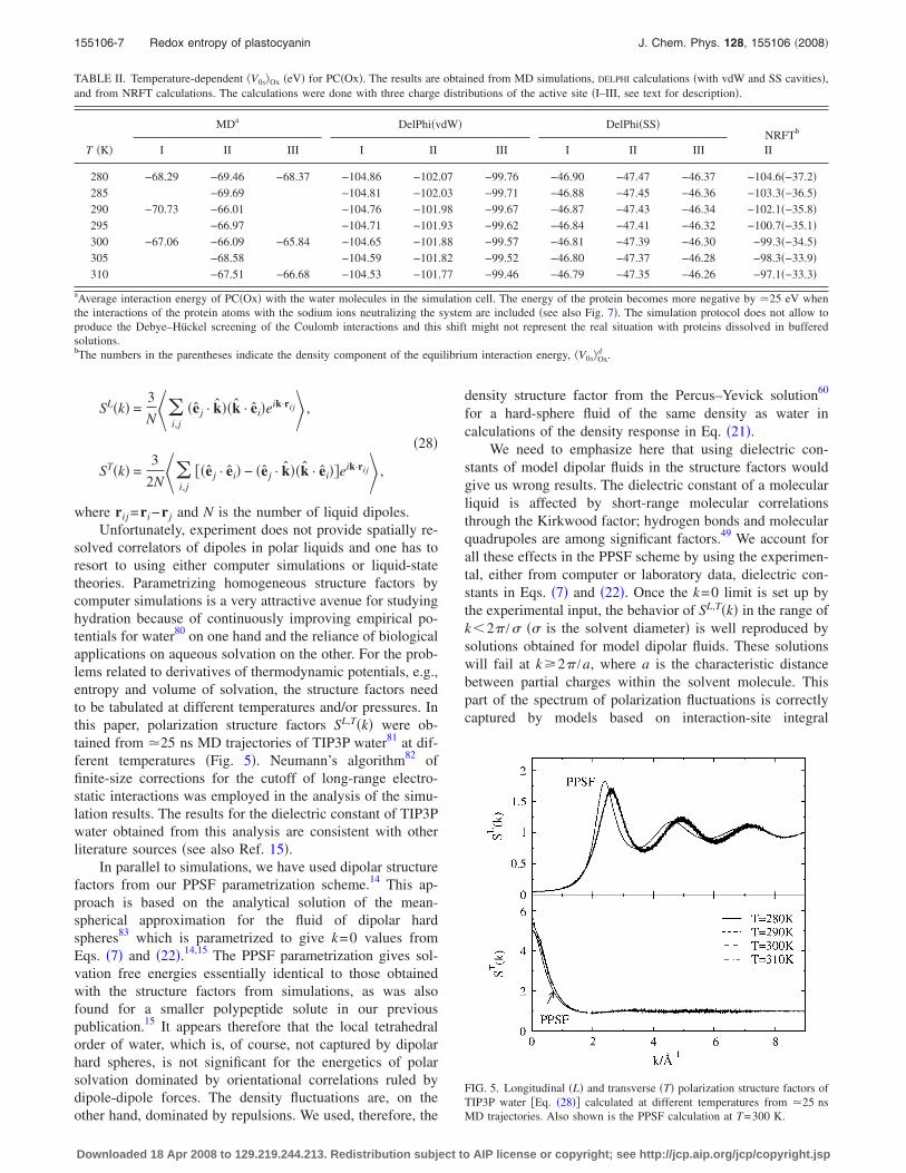
solved correlators of dipoles in polar liquids and one has toresort to using either computer simulations or liquid-statetheories. Parametrizing homogeneous structure factors bycomputer simulations is a very attractive avenue for studyinghydration because of continuously improving empirical po-tentials for water80 on one hand and the reliance of biologicalapplications on aqueous solvation on the other. For the prob-lems related to derivatives of thermodynamic potentials, e.g.,entropy and volume of solvation, the structure factors needto be tabulated at different temperatures and/or pressures. Inthis paper, polarization structure factors SL,T�k� were ob-tained from �25 ns MD trajectories of TIP3P water81 at dif-ferent temperatures �Fig. 5�. Neumann’s algorithm82 offinite-size corrections for the cutoff of long-range electro-static interactions was employed in the analysis of the simu-lation results. The results for the dielectric constant of TIP3Pwater obtained from this analysis are consistent with otherliterature sources �see also Ref. 15�.

In parallel to simulations, we have used dipolar structurefactors from our PPSF parametrization scheme.14 This ap-proach is based on the analytical solution of the mean-spherical approximation for the fluid of dipolar hardspheres83 which is parametrized to give k=0 values fromEqs. �7� and �22�.14,15 The PPSF parametrization gives sol-vation free energies essentially identical to those obtainedwith the structure factors from simulations, as was alsofound for a smaller polypeptide solute in our previouspublication.15 It appears therefore that the local tetrahedralorder of water, which is, of course, not captured by dipolarhard spheres, is not significant for the energetics of polarsolvation dominated by orientational correlations ruled bydipole-dipole forces. The density fluctuations are, on theother hand, dominated by repulsions. We used, therefore, the

density structure factor from the Percus–Yevick solution60

for a hard-sphere fluid of the same density as water incalculations of the density response in Eq. �21�.

We need to emphasize here that using dielectric con-stants of model dipolar fluids in the structure factors wouldgive us wrong results. The dielectric constant of a molecularliquid is affected by short-range molecular correlationsthrough the Kirkwood factor; hydrogen bonds and molecularquadrupoles are among significant factors.49 We account forall these effects in the PPSF scheme by using the experimen-tal, either from computer or laboratory data, dielectric con-stants in Eqs. �7� and �22�. Once the k=0 limit is set up bythe experimental input, the behavior of SL,T�k� in the range ofk�2� /� �� is the solvent diameter� is well reproduced bysolutions obtained for model dipolar fluids. These solutionswill fail at k�2� /a, where a is the characteristic distancebetween partial charges within the solvent molecule. Thispart of the spectrum of polarization fluctuations is correctlycaptured by models based on interaction-site integral

TABLE II. Temperature-dependent �V0s�Ox �eV� for PC�Ox�. The results are obtained from MD simulations, DELPHI calculations �with vdW and SS cavities�,and from NRFT calculations. The calculations were done with three charge distributions of the active site �I–III, see text for description�.

T �K�

MDa DelPhi�vdW� DelPhi�SS�NRFTb

III II III I II III I II III

280 −68.29 −69.46 −68.37 −104.86 −102.07 −99.76 −46.90 −47.47 −46.37 −104.6�−37.2�285 −69.69 −104.81 −102.03 −99.71 −46.88 −47.45 −46.36 −103.3�−36.5�290 −70.73 −66.01 −104.76 −101.98 −99.67 −46.87 −47.43 −46.34 −102.1�−35.8�295 −66.97 −104.71 −101.93 −99.62 −46.84 −47.41 −46.32 −100.7�−35.1�300 −67.06 −66.09 −65.84 −104.65 −101.88 −99.57 −46.81 −47.39 −46.30 −99.3�−34.5�305 −68.58 −104.59 −101.82 −99.52 −46.80 −47.37 −46.28 −98.3�−33.9�310 −67.51 −66.68 −104.53 −101.77 −99.46 −46.79 −47.35 −46.26 −97.1�−33.3�

aAverage interaction energy of PC�Ox� with the water molecules in the simulation cell. The energy of the protein becomes more negative by �25 eV whenthe interactions of the protein atoms with the sodium ions neutralizing the system are included �see also Fig. 7�. The simulation protocol does not allow toproduce the Debye–Hückel screening of the Coulomb interactions and this shift might not represent the real situation with proteins dissolved in bufferedsolutions.bThe numbers in the parentheses indicate the density component of the equilibrium interaction energy, �V0s�Ox

d .

FIG. 5. Longitudinal �L� and transverse �T� polarization structure factors ofTIP3P water �Eq. �28�� calculated at different temperatures from �25 nsMD trajectories. Also shown is the PPSF calculation at T=300 K.



equations,39 but that range of wave vectors normally does notcontribute to the solvation energy. In fact, the range of kvalues relevant for the solvation problem is limited byk�2� /R, where R is the characteristic dimension of the sol-ute. For large solutes, only the long-wavelength part of thepolarization structure factors is really needed for the solva-tion energy calculations. As is shown in Fig. 5, there is amismatch between the PPSF longitudinal structure factor andMD simulations. However, this difference makes no effecton the calculated solvation energies.

We can summarize our results on parametrizing the sol-vent properties by stating that the model fluid of dipolar hardspheres can serve as a reliable reference system for calculat-ing polar solvation given the macroscopic properties, thedensity of dipoles y and the dielectric constant s, have beentaken from experiment �either laboratory or computer�. Thetheory thus adds an additional parameter y to the dielectricconstant used in electrostatic solvation theories to produce afully microscopic solvent response. In practical applicationsof the theory �e.g., in case of solvation in ambient waterpresented below�, the parameter y needs to be calculatedfrom the molecular properties of the solvent. We use the 1-RWertheim theory84 to calculate the effective dipole momentof the solvent �see Ref. 85 for comparison to simulations�.The solvent input is thus made by five parameters:�� ,� ,m , ,s�. One needs, in addition, the high-frequencydielectric constant for the reorganization energy calcula-tions and the temperature slopes of two dielectric constants,as well as the isobaric expansivity of the solvent, for thesolvation entropy calculations. The big advantage of thePPSF scheme is that all these parameters have been tabulatedfor many solvents commonly used in solution chemistrymaking our method broadly applicable to solvation calcula-tions in polar molecular solvents.

Despite the fact that the dielectric constant is sensitive tolocal correlations, the polarization structure factors in thelong-wavelength limit are fully determined by dipolar corre-lations general for all polar liquids and not much sensitive todetails of the local structure which is, of course, very differ-ent in water than in a hard-sphere dipolar fluid. There areseveral advantages to using dipolar hard spheres as the ref-erence system. First, all thermodynamic and structural prop-erties are controlled by only two parameters, the reduceddensity ��3 and the dipolar density y. Second, this systemhas been well characterized both analytically and numeri-cally. It has served many times as a starting point for devel-oping theories of polar liquids,60 similarly to the role playedby the fluid of hard spheres in theories of nonpolar liquids.53

Once that stated, we, however, want to stress that the theoryitself is based on the structure factors of an arbitrary polarmedium with the Gaussian fluctuation spectrum and is notlimited to a choice of any particular reference system.

IV. SIMULATIONS PROTOCOL

AMBER 8.0 �Ref. 86� was used for all MD simulations.The initial configuration of PC was created using a proto-nated version of the x-ray crystal structure at 1.7 Å reso-lution �PDB: 1ag6, Ref. 87�. This initial configuration of the

protein was first minimized in vacuum by the conjugate gra-dient method for 10 000 steps to allow the protein to removeany bad initial contacts. Then the system was solvated in arectilinear box with several thousand TIP3P molecules,81

providing at least two to three solvation shells around theprotein. To neutralize the charge, a number of sodium ionsequal to the total charge of the protein were added. The pro-tein was then relaxed for a few thousand steps while waterand sodium were positionally constrained. Finally, the entiresystem containing solvent, counterions, and protein wasenergy minimized in 100 000 steps.

Next, the system was heated in a NVT ensemble for30 ps from 0 K to the desired temperature followed by vol-ume expansion in a 1 ns NPT run. NVT production runs,following density equilibration, lasted from 6 to 18 ns. Thelast 5–10 ns at the end of each trajectory were used to cal-culate the averages. The timestep for all MD simulations was2 fs, and SHAKE was employed to constrain bonds to hy-drogen atoms. Constant pressure and temperature simula-tions employed Berendsen barostat and thermostat,respectively.88 The long-range electrostatic interactions werehandled using a smooth particle mesh Ewald summationwith a 9 Å limit in the direct-space sum. The total charge forthe protein was −9.0 for the reduced state and −8.0 for theoxidized state.

The MD trajectories were produced in parallel runs atASU’s HPC facility and required 4.0–4.5 years of CPU timefor collecting the simulation data followed by 1.8–2.0 yearsof the analysis. The analysis was also done in parallel on theOpteron cluster using a parallel code developed for thisproject which directly reads binary AMBER files.

V. RESULTS

The calculations presented here are focused on twoproperties: The solvent portion of the redox chemicalpotential, ��s, and the solvent reorganization energy �s, bothcorresponding to the half reaction

PC�Ox�8− + e− → PC�Red�9−. �29�

The former can in principle be calculated as the difference ofsolvation chemical potentials in the Red and Ox states. How-ever, this approach involves calculating the difference in twolarge numbers, which is computationally unreliable. Instead,we use the linear response approximation to calculate ��s

according to the equation

��s = �0sRed − �0s

Ox = − �E0 � � � E0. �30�

Here, E0= �E0Ox+ E0

Red� /2 and �E0= E0Red− E0

Ox are the meanand the difference of the electric fields in the Red and Oxstates. Similarly, the solvent reorganization energy iscalculated from

�s = 12�E0 � � � �E0. �31�

Equation �31� applies to the reorganization energy of nonpo-larizable solvents employed in computer simulations. Forlaboratory data, nuclear polarization should be separatedfrom the overall solvent polarization and the response



function � is replaced by the nuclear response function �n asexplained above and in more detail in Ref. 15.

A. Redox thermodynamics

The solvation thermodynamics calculated here can berelated to experimental redox entropies reported by measur-ing the temperature dependence of the standard or midpointelectrode potentials.24,25,35 An electrochemical experimentcorresponds to bringing a solution containing given numbersof oxidized and reduced reagents, which are not necessarilyin equilibrium �the ratio of their numbers is not a Boltzmannfactor�, in contact with a metal electrode. The equilibrium isestablished between the electronic subsystem of the redoxpair and the electrode in such a way that the electrode ischarged and its electrochemical potential � is shifted fromthe vacuum Fermi energy F by the electrostatic potential�: �=F−e�.

The numbers of the oxidized and reduced forms of theredox pair, NOx and NRed, are assumed to be large enough sothat they are not affected by charging the electrode. The elec-trochemical potential of the electrode than becomes equal tothe absolute electrochemical potential of the redox couple inthe solution.89 The latter can be found from simple statisticalarguments. The grand-canonical free energy of twofermionic subsystems of NOx and NRed electronic levels is90

�� = − NOx ln�1 + e��−Ox�� − NRed ln�1 + e��−Red�� ,

�32�

where Ox and Red are the average energies of the electroniclevels in the corresponding redox states. The chemical poten-tial is then found by requiring that the derivative −�� /��T

is equal to the total number of electrons NRed. For the energygap between Ox and Red states greater than kBT, thisrequirement results in the Nernst equation,91

� =Ox + Red

2− kBT ln�NOx/NRed� , �33�

in which the standard potential is given by the mean of theaverage electronic energies

�0 = −Ox + Red

2e. �34�

The same result follows from the use of the stationarycondition �zero electrode current� for the rates of reductionand oxidation92

kOxcOx = kRedcRed, �35�

where cOx/Red are the surface concentrations. By using theMarcus equation for the reaction rate,93

kOx/Red � exp�− ��Ox/Red − ��2

4�s� , �36�

and neglecting the logarithmic correction including the ratioof two surface concentrations, one gets equal rates at��Ox+Red� /2. The double-well Marcus free energy sur-face for the electrode electron transfer is then symmetrical asillustrated in Fig. 6. This picture bears a clear similarity with

the formation of the Fermi level in the forbidden band of asemiconductor, as was noticed by Reiss.94

The electronic energies are given by the sums of theirvacuum components, Ox/Red

0 , and the interaction of the elec-tric field of the electron Ee with the polarization of thesolvent in equilibrium with the total electric field of themolecule in the solution,95

Ox/Red = Ox/Red0 − Ee � � � E0

Ox/Red. �37�

Taking into account that

Ee = E0Red − E0

Ox = �E0, �38�

one gets from Eqs. �34�, �37�, and �38� the commonly usedconnection between the standard electrode potential and thesolvation part of the redox free energy,

�0 = −Red

0 + Ox0

2e−

��s

e, �39�

where ��s is given by Eq. �30�. The first term in this equa-tion disappears in the temperature derivative reportedexperimentally,24–26

e ��0

�T�

P= �ss = ss

Red − ssOx = − ��s

�T�

P. �40�

We need to stress here that redox entropies in polar solutionsare sensitive to the presence of electrolyte.22,96 One thereforecan expect only a qualitative agreement between experimentsdone in buffered protein solutions25,26 and our calculations atzero ionic strength.

From Eqs. �34�, �37�, and �38�, one can directly derivethe equation for the solvation redox free energy,

��s = ��V0s�Ox + ��V0s�Red�/2, �41�

where �V0s is the difference in the solute-solvent interactionenergies in the Red and Ox states and the averages are takenover the corresponding ensembles. The same average verticalgaps can be used to calculate the reorganization energy as

FIG. 6. Contact of a redox pair with the metal electrode. Ox−� and Red

−� show the fluctuating energy gaps for reduction and oxidation electrontransfer, respectively. The equilibrium electrochemical potential of the elec-trode is established when the equilibrium energy gaps are equal for thereduction and oxidation reactions �Eq. �33��. The Marcus electron transferparabolas, shown by the dependence of free energy F�X� on the energy gapcoordinate X=Ox−�, are symmetric in this case producing equal oxidationand reduction currents �Eq. �35��.



�s = ��V0s�Ox − ��V0s�Red�/2. �42�

We need to caution here that, while Eq. �34� is a statistical-mechanical result, Eqs. �37� and �42� are based on the LRAfor the solute-solvent interaction energy and might be af-fected by deviations from this approximation.

B. Solute-solvent average energy

In addition to our NRFT formalism, we have used thedielectric continuum approximation implemented in theDELPHI program suite7 in the solvation calculations. Dielec-tric constant of ambient water was used for the solvent con-tinuum and s=1 for the protein. This latter choice wasdriven by our desire to compare continuum and microscopiccalculations of solvation thermodynamics since the latterdoes not assume any polarization of the protein. Three dif-ferent charging schemes have been used and compared toMD simulations �Table I and Sec. IV�. In the following, wewill discuss the results relevant to charging scheme II only,which are also visualized in Fig. 7. Table II lists the results ofNRFT and DELPHI calculations of the average energy �V0s�Ox

of PC in the Ox state, where V0s refers to the interaction ofthe protein with the water molecules in the simulation box.Sodium ions used to neutralize the simulation box shift theinteraction potential down by about −25 eV as is shown byopen circles in Fig. 7. It is not clear how realistic this numbermight be since Debye–Hückel screening is not accounted forby the simulations. In addition, we found that the variance ofthe Coulomb interactions with the counterions is negligiblethus resulting in a very small contribution to the reorganiza-tion energy, which is known to be the case from analyticalmodels which do include the Debye–Hückel screening.97

The NRFT calculations listed in Table II and shown inFig. 7 have been done by using Eqs. �3� and �9� in which the

electric field of PC in Ox state was used for E0�k�. The closediamonds in Fig. 7 refer to the total solvent response, whileopen diamonds represent the polarization response only��p in Eq. �9��. Two interesting observations result from ex-amining Fig. 7: �i� A close proximity of the NRFT result tothe standard �vdW� continuum calculation and �ii� a goodagreement between the polarization portion of the NRFT cal-

culations and MD results. The continuum electrostatics doesnot reproduce the slope of the average energy as we alsodiscuss below in relation to the redox entropy.

In order to understand the origin of the close agreementbetween MD and the polarization component of the solventresponse, one needs to recall what comes to the calculationof the polarization and density components of the solvationfree energy. The polarization response is calculated by as-suming that the only influence of the solute on the polariza-tion field is to exclude it from the solute volume representedby the step function �0�r� equal to one inside the solute andzero otherwise �Eq. �12��. The density component correctsthis result by taking into account the inhomogeneous densityprofile formed at the surface of a hard-wall solute. In denseliquids, such a profile is characterized by a sharp peak of theradial distribution function in the first solvation shell of thesolute. Correspondingly, reflecting the belief that the short-range structure of liquids is primarily determined byrepulsions,53 the density structure factor S�k� in Eq. �21� wastaken in our calculations from the Percus–Yevick solution forhard spheres.60 The close proximity of the full NRFT calcu-lation to the standard DELPHI/vdW algorithm �Fig. 7� illus-trates the fact that the common parametrization of the atomicradii is based on the experience learned for hydration ofsmall ions with tightly bound first solvation shell. In thepresent algorithm, this physics is accommodated by the den-sity component of the solvation free energy.

The structure of water at the protein surface is quitedifferent from what is normally obtained by inserting a smallsolute in a molecular solvent. The structure is inhomoge-neous, including islands of highly structured water aroundpolar and ionized residues and a much softer density profileat the hydrophobic patches. This reality is illustrated in Fig. 8which shows pair distribution functions between ionized and

FIG. 7. Average solute-solvent interaction energy �V0s�Ox obtained from MDsimulations �closed circles�, NRFT �diamonds�, and DELPHI continuum cal-culations �vdW cavity, triangles�. The closed diamonds refer to the totalaverage energy including the polarization and density components, while theopen diamonds denote the polarization component only. The dashed linesrepresent linear regressions through the points.

FIG. 8. Radial distribution functions between surface residues of PC andoxygens of water. The upper panel shows ionized residues and the lowerpanel refers to nonpolar residues. The legends in the figure list. aspartic acid�ASP�, the probe atom is the oxygen at the first � position; lysine �LYS�, theprobe atom is nitrogen at the � position; proline �PRO�, the probe atom isthe � carbon; tyrosine �TYR�, with the first carbon as the probe atom.



non-polar residues and water’s oxygens. While the distribu-tion functions of ionized residues are reminiscent of thestructures typically observed around small solutes in densesolvents, the water structure around nonpolar residues isquite different: There is no first shell peak and water inter-face is shifted by �1 Å, in accord with simulations of nanos-cale hydrophobic solutes.98

The stronger attraction of the surface water molecules tothe bulk than to a nonpolar hydrophobic patch of the protein�cavity expulsion potential99,100� results in a weak dewettingof the surface19 with the density at the interface lower than inthe bulk �Fig. 8�. Since there are only a few charged residueson the protein surface �see the Discussion section�, the aver-age surface structure is closer to a stepwise cutoff introducedin the polarization component of the response function thanto a structured liquid at the surface of a small polar/ionicsolute.101 This observation explains a good agreement be-tween MD and polarization calculations of the solvation ther-modynamics in this paper as well as an equally impressiveagreement with the simulations obtained in our previous cal-culations of charge transfer across a polypeptide bridge.15

C. Solvent Gibbs and reorganization free energies

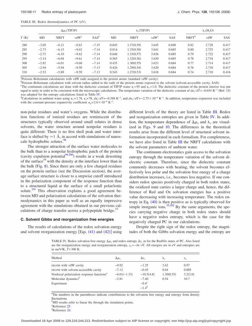
The results of calculations of the redox solvation energyand solvent reorganization energy �Eqs. �41� and �42�� using

different levels of the theory are listed in Table III. Redoxand reorganization entropies are given in Table IV. In addi-tion, the temperature dependence of ��s and �s are visual-ized in Figs. 9 and 10. The differences in the theoreticalresults arise from the different level of structural solvent in-formation incorporated in each formalism. For completeness,we have also listed in Table III the NRFT calculations withthe solvent parameters of ambient water.

The continuum electrostatics gain access to the solvationentropy through the temperature variation of the solvent di-electric constant. Therefore, since the dielectric constantcommonly decreases with heating, the solvent becomes ef-fectively less polar and the solvation free energy of a chargedistribution increases, i.e., becomes less negative. If one con-siders redox species positively charged in both redox states,the oxidized state carries a larger charge and, hence, the dif-ference of Red and Ox solvation energies has a positivevalue decreasing with increasing temperature. The redox en-tropy in Eq. �40� is then positive as is typically observed forsimple inorganic ions.35,102 By the same arguments, the spe-cies carrying negative charge in both redox states shouldhave a negative redox entropy, which is the case for thenegatively charged PC in our calculations.

Despite the right sign of the redox entropy, the magni-tudes of both the Gibbs solvation energy and the entropy are

TABLE III. Redox thermodynamics of PC �eV�.

T �K�

��s�TIP3P� �s�TIP3P� �s�H2O�

MD NRFT vdWa SASb MD NRFT vdWc SAS NRFTd vdW SAS

280 −3.05 −6.21 −9.63 −7.15 0.845 1.37�0.59� 3.645 0.690 0.82 2.728 0.417285 −2.73 −6.15 −9.62 −7.14 0.814 1.35�0.58� 3.641 0.685 0.80 2.725 0.417290 −2.71 −6.10 −9.62 −7.14 0.646 1.33�0.57� 3.636 0.685 0.79 2.722 0.417295 −3.14 −6.04 −9.61 −7.14 0.565 1.32�0.56� 3.630 0.685 0.78 2.718 0.417300 −2.82 −6.01 −9.60 −7.14 0.435 1.30�0.55� 3.623 0.684 0.77 2.714 0.417305 −2.94 −5.94 −9.59 −7.13 0.426 1.29�0.54� 3.620 0.684 0.76 2.710 0.417310 −2.53 −5.89 −9.59 −7.13 0.543 1.27�0.53� 3.618 0.684 0.74 2.710 0.416

aPoisson–Boltzmann calculations with vdW radii assigned to the protein atoms �standard vdW cavity�.bPoisson–Boltzmann calculation with solvent radius added to the radii of the protein atoms exposed to the solvent �solvent-accessible cavity, SAS�.cThe continuum calculations are done with the dielectric constant of TIP3P water s=95 and =1.0. The dielectric constant of the protein interior was putequal to unity in order to be consistent with the microscopic calculations. The temperature variation of the dielectric constant of ds /dT=−0.654 K−1 �Ref. 15�was adopted for the entropy calculations listed in Table IV.dCalculations in ambient water using =1.78, s=78, ds /dT=−0.398 K−1, and d /dT=−2.75�10−4 K−1. In addition, temperature expansion was includedwith the constant pressure expansivity coefficient p=2.6�10−4 K−1.

TABLE IV. Redox solvation free energy ��s and redox entropy �ss in for the Red/Ox states of PC. Also listedare the reorganization energy and reorganization entropy, s�=−�� /�T. All energies are in eV and entropies arein meV/K, T=300 K.

Method ��s �ss �s s�

DELPHI with vdW cavity −9.92 −1.25 3.62 0.97DELPHI with solvent-accessible cavity −7.12 −0.45 0.64 0.005Nonlocal polarization response functionsa −6.01�−1.33� −10.5�4.8� 1.30�0.55� 3.2�2.0�Molecular dynamicsb −2.81 −7.40 0.54 10.7Experiment −0.4c

−1.4d

aThe numbers in the parentheses indicate contributions to the solvation free energy and entropy from densityfluctuations.bMD results refer to linear fits through the simulation points.cReference 25.dReference 24.



markedly different in continuum and microscopic/simulationapproaches: ��s is higher in the standard implementationof DELPHI �vdW cavity� than the NRFT value by a factor of1.5 while the redox entropy is lower by a factor of ten. Theuse of the solvent-accessible cavity brings the value of ��s

in a closer proximity to the NRFT, but the redox entropy islowered even more �Table IV�. The magnitude of ��s fromNRFT is significantly higher than from MD even if the den-sity component is subtracted from the total response. Thisinitially comes a bit of surprise given a good agreement be-tween the polarization-NRFT and MD values of �V0s�Ox re-ported in Table II and Fig. 7. We do not currently have agood explanation of this disagreement �see Discussionbelow�.

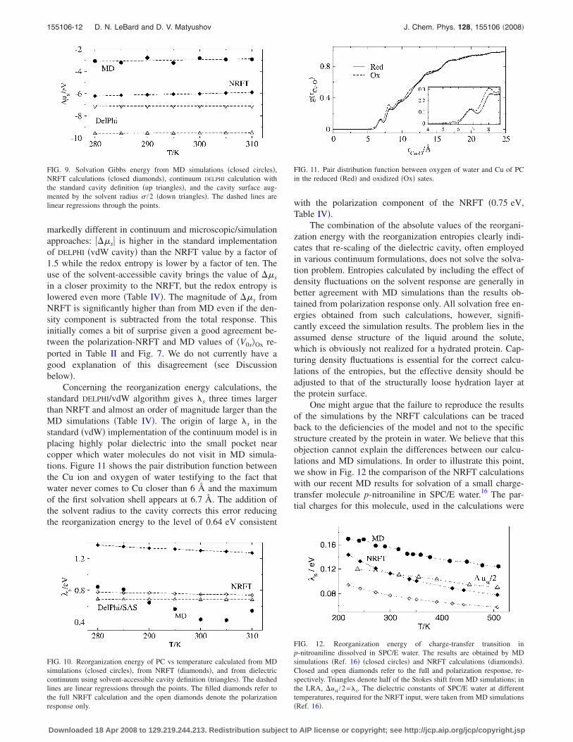
Concerning the reorganization energy calculations, thestandard DELPHI/vdW algorithm gives �s three times largerthan NRFT and almost an order of magnitude larger than theMD simulations �Table IV�. The origin of large �s in thestandard �vdW� implementation of the continuum model is inplacing highly polar dielectric into the small pocket nearcopper which water molecules do not visit in MD simula-tions. Figure 11 shows the pair distribution function betweenthe Cu ion and oxygen of water testifying to the fact thatwater never comes to Cu closer than 6 Å and the maximumof the first solvation shell appears at 6.7 Å. The addition ofthe solvent radius to the cavity corrects this error reducingthe reorganization energy to the level of 0.64 eV consistent

with the polarization component of the NRFT �0.75 eV,Table IV�.

The combination of the absolute values of the reorgani-zation energy with the reorganization entropies clearly indi-cates that re-scaling of the dielectric cavity, often employedin various continuum formulations, does not solve the solva-tion problem. Entropies calculated by including the effect ofdensity fluctuations on the solvent response are generally inbetter agreement with MD simulations than the results ob-tained from polarization response only. All solvation free en-ergies obtained from such calculations, however, signifi-cantly exceed the simulation results. The problem lies in theassumed dense structure of the liquid around the solute,which is obviously not realized for a hydrated protein. Cap-turing density fluctuations is essential for the correct calcu-lations of the entropies, but the effective density should beadjusted to that of the structurally loose hydration layer atthe protein surface.

One might argue that the failure to reproduce the resultsof the simulations by the NRFT calculations can be tracedback to the deficiencies of the model and not to the specificstructure created by the protein in water. We believe that thisobjection cannot explain the differences between our calcu-lations and MD simulations. In order to illustrate this point,we show in Fig. 12 the comparison of the NRFT calculationswith our recent MD results for solvation of a small charge-transfer molecule p-nitroaniline in SPC/E water.16 The par-tial charges for this molecule, used in the calculations were

FIG. 9. Solvation Gibbs energy from MD simulations �closed circles�,NRFT calculations �closed diamonds�, continuum DELPHI calculation withthe standard cavity definition �up triangles�, and the cavity surface aug-mented by the solvent radius � /2 �down triangles�. The dashed lines arelinear regressions through the points.

FIG. 10. Reorganization energy of PC vs temperature calculated from MDsimulations �closed circles�, from NRFT �diamonds�, and from dielectriccontinuum using solvent-accessible cavity definition �triangles�. The dashedlines are linear regressions through the points. The filled diamonds refer tothe full NRFT calculation and the open diamonds denote the polarizationresponse only.

FIG. 11. Pair distribution function between oxygen of water and Cu of PCin the reduced �Red� and oxidized �Ox� sates.

FIG. 12. Reorganization energy of charge-transfer transition inp-nitroaniline dissolved in SPC/E water. The results are obtained by MDsimulations �Ref. 16� �closed circles� and NRFT calculations �diamonds�.Closed and open diamonds refer to the full and polarization response, re-spectively. Triangles denote half of the Stokes shift from MD simulations; inthe LRA, �ust /2=�s. The dielectric constants of SPC/E water at differenttemperatures, required for the NRFT input, were taken from MD simulations�Ref. 16�.



tabulated in Ref. 103. The comparison with the NRFTmethod is somewhat complicated in this case by nonlinearsolvation effects related to specific binding of water to theoxygen sites and seen in the deviation of the half of theStokes shift from the reorganization energy. Nevertheless,the NRFT calculation with the density component included isin a reasonable agreement with the simulation data for boththe reorganization energy and entropy, while the polarizationresponse alone clearly underestimates the reorganizationenergy.

VI. DISCUSSION

This paper has addressed the thermodynamics of electro-static interactions of the protein with water. The free energyof electrostatic protein/water coupling is a part of the overallfree energy of protein solvation. This component is experi-mentally probed by changing the charge of the redox site inredox reactions. What has been left out from our analysis isthe electrostatic interaction of the active site with the proteincharges. This component is probably less significant for theredox entropy �see below�, but needs to be included into acomplete analysis of the redox thermodynamics. The exten-sion of the present algorithm to this case is currently delayedby the absence of reliable models of microscopic polariza-tion correlation functions of the protein. Once these areavailable, the formalism can be extended to include proteinelectrostatics. Our hope for this development is based on theobservation, from our current simulations, that the cross cor-relation of interaction potentials of the redox site with waterand protein is small �approximately 10%� �Ref. 104� in theoverall cumulant ��V0s�2� allowing one to treat, in the firstapproximation, the protein and water cumulants separately.

The formalism developed here is based on the LRA sug-gesting that knowing the variance of electrostatic fluctuationsaround a neutral repulsive solute is sufficient to calculate thesolvation chemical potential �Eq. �2��. One can arrive at Eq.�2� from the following simple considerations. The chemicalpotential of solvation can be written as the integral over themagnitude of the solute-solvent electrostatic interaction=V0s as follows:

e−��0s = dP�,��e−�. �43�

Here, the probability density P� ,�� of reaching the value is obtained by taking the statistical average over the refer-ence Hamiltonian H0 which includes all the interactionpotentials in the system except the solute-solvent electro-static potential V0s,

P�,�� = Q0−1 �� − V0s�e−�H0d� , �44�

where Q0=� exp�−�H0�d� and � denotes the phase spacevolume.90 Since the solute-solvent component of H0 includesmostly isotropic short-range interactions, one can put �V0s�0

=0. In addition, the Gaussian approximation can be appliedto P� ,��,

P�,�� exp�−2

2�2� , �45�

with

�2 = ��V0s�2�0. �46�

Combining Eqs. �43� and �45�, one immediately arrives atEq. �2�.

One of the important lessons of Eqs. �43� and �44� is thatall the thermodynamic information required for the solvationproblem is contained in the distribution of electrostatic po-tential fluctuations around a “nonpolar” solute in which allthe electrostatic interactions with the solvent have beenswitched off. For large solutes, the spectrum of electrostaticfluctuations around the repulsive solute core will ultimatelydetermine the thermodynamics of solvation. The Gaussianityof electrostatic fluctuations created by polar solvents insidenonpolar solutes �Eq. �45�� still needs testing, in particular atlarge scale, since it was questioned for small solutesdissolved in water.105 However, it is important to stress thatEqs. �43� and �44� are exact and not limited to linearsolvation.

The reasoning outlined above works well for small- andmedium-size solutes, as is exemplified in Fig. 12. However,the application of the same procedure to protein solvationstudied in this paper has encountered some difficulties sug-gesting that methods developed over several decades andsuccessfully applied to solvation of small solutes in densepolar solvents are probably not directly transferable withoutsignificant modifications to mesoscopic hydration of pro-teins. The application of our algorithm to the calculation ofthe average solute-solvent interaction energy turned out to bequite successful when the density profile of water around theprotein is approximated by a step function �Fig. 7�. The cal-culations agree with MD within simulation uncertainties��5% �. As mentioned above, this comes as a result of av-eraging between tight and loose water structures at the pro-tein surface. The application of the same procedure to solva-tion of the difference charges of the active site�reorganization energy, Fig. 10� was less successful, but theagreement is probably still acceptable, in particular, at lowesttemperatures.

Where the calculations and simulations come in signifi-cant disagreement is for the free energy of solvation obtainedin simulations as the mean of two vertical transition energies�Eq. �41��. Some recent simulations of cavities in force-fieldwater models106,107 and of uncharged protein108 have sug-gested a possible origin of this effect. It was found that waterstructured at the protein surface creates a positive potentialwithin an uncharged cavity/protein. In terms of Eq. �45�, thisimplies a constant shift of the solute-solvent energy →−0. Since we have assumed random orientations of wateraround an uncharged solute, as is indeed the case for smallsolutes,16 our calculations do not include the effect of a posi-tive background potential and include only changes of thepotential in response to protein’s charges. In the case of aconstant background potential �, Eq. �41� modifies to



��s = ��V0s�Ox + ��V0s�Red�/2 − �q� , �47�

where �q=qRed−qOx=−1. Ashbaugh106 reported an averagepositive potential of about e��9 kcal /mol for cavities inSPC water comparable in size with PC. In terms of our cal-culations, it amounts a positive shift of the simulation databy about 0.4 eV which will increase the current gap of about3.2 eV �300 K� between the MD and NRFT.

The origin of the difference in solvation free energiesbetween calculations and MD simulations might be related tothe weakly dewetted water density profile near the activesite. This would imply that some of the properties of waterstructure around large cavities expelled by the protein fromits volume are quite different from the common experiencegained with small solutes. This qualitative difference be-tween small-size and large-size solvation has recently gainedappreciation for hydrophobic solvation101 as we discuss next.

The Gaussian model of hydrophobic solvation goes backto the Pratt–Chandler theory of hydrophobicity109 recentlyextended by Pratt and co-workers.110,111 The formulation ofthe theory of hydrophobic solvation follows a path similar tothe one outlined in Eqs. �43�–�46� asking what is the freeenergy �� needed to solvate a solute of volume �0. It isgiven by the Gaussian probability,101,110

�� 2�0

2

2��

, �48�

with the fluctuation of the number of solvent particles involume �0,

�� = ��N�2�� = ��0 + �2�0

drdr�hss�r − r�� . �49�

In Eq. �49�, hss�r� is the pair correlation function of thehomogeneous solvent.

The Gaussian probability of electron transfer carries aclose similarity with Eq. �48� giving the activation freeenergy as

��act =X0

2

2�2 , �50�

where X0 is the average vertical donor-acceptor energy gapand �

2 is the variance of the solute-solvent interaction po-tential when V0s=�V0s is used in Eqs. �44� and �45�. Notsurprisingly, the structure of the equation for �

2 resemblesEq. �49�:

�2 = � V0s

2 �1�d�1 + �2 V0s�1�V0s�2�hss�1,2�d�1d�2

+ �2 V0s2 �1�hss�1,2��0�2�d�1d�2. �51�

The last summand in this equation represents the densitycomponent of the response since it transforms into thek-space integral with the density structure factor of the liquid�Eq. �21��.

Equation �51� carries a close resemblance with thePratt-Chandler theory of hydrophobicity.109 The sum of the

first and the third terms is the average of the squared solute-solvent potential V0s

2 �1� over the solute-solvent densityprofile,112

��r� = ��1 + c0s�r�� + �2 c0s�r��hss�r − r��dr�, �52�

in which the solute-solvent direct correlation functionc0s�r� is replaced by its lowest density expansion,60 c0s�r��−�0�r� ��0�r� is one inside the solute and zero otherwise�.The observation that the density profile around solutes ofsize �1 nm can be approximated by a step function �Fig. 11,also see Fig. 3 in Ref. 101� amounts to neglecting the secondterm in Eq. �52� and, correspondingly, the density compo-nents �d in the solvent response function �Eq. �9��.

The fact that the spectrum of electrostatic potential fluc-tuations around a nonpolar solute gives complete informationabout polar solvation brings this latter problem in close rela-tion to the problem of hydrophobic solvation. It was realizedin recent years that hydrophobic solvation of small and largesolutes are qualitatively different.19,101,112 Solvation characterchanges at the critical size of �1 nm from entropy-dominated solvation of small solutes �Gaussian statistics110�to enthalpy-dominated solvation of large solutes driven bythe creation of the solute-solvent interface �non-Gaussianstatistics113�. The solvent interface around large solutes in-volves partial dewetting, strongly sensitive to the strength ofsolute-solvent attractions17 and the appearance of large-sizeinterfacial density fluctuations.101 In case of protein solva-tion, surface water creates a nonzero potential around un-charged proteins discussed above, while density fluctuationslead to complex protein-solvent dynamics18 and are probablyconnected to “slaving” of the protein dynamics by thesolvent.114

The inhomogeneous nature of the protein/water interfaceis illustrated in Fig. 13. The inset in the figure shows thedistribution of distances between charged residues at the pro-tein surface with the average of about 17 Å. This distance issufficient for a buildup of partially dewetted water structuresat the hydrophobic surface between the charges, with thecritical distance estimated to be about 1 nm.101 Figure 13

FIG. 13. The distribution of binding energies of water molecules in the firstsolvation shell of PC�Ox� defined by adding the water diameter 2.87 Å to allprotein atoms exposed to solution. The binding energy is defined as the totalinteraction energy of a given water molecule with all atoms of the protein.The inset shows the distribution of distances of charged residues at theprotein surface.



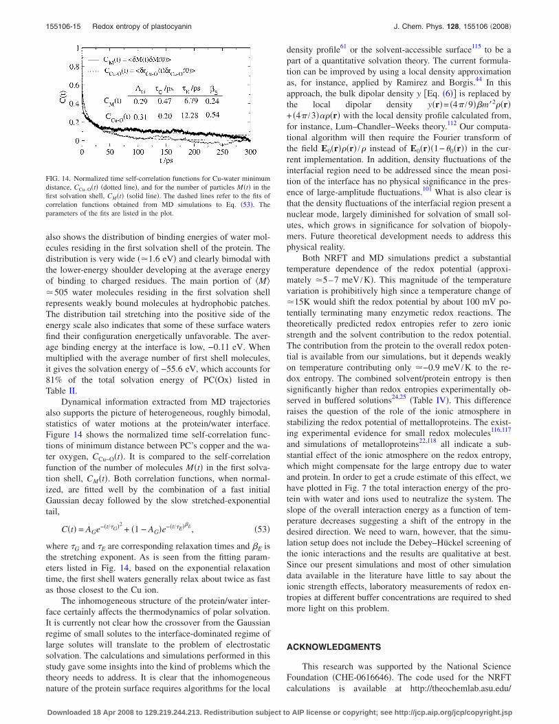
also shows the distribution of binding energies of water mol-ecules residing in the first solvation shell of the protein. Thedistribution is very wide ��1.6 eV� and clearly bimodal withthe lower-energy shoulder developing at the average energyof binding to charged residues. The main portion of �M��505 water molecules residing in the first solvation shellrepresents weakly bound molecules at hydrophobic patches.The distribution tail stretching into the positive side of theenergy scale also indicates that some of these surface watersfind their configuration energetically unfavorable. The aver-age binding energy at the interface is low, −0.11 eV. Whenmultiplied with the average number of first shell molecules,it gives the solvation energy of −55.6 eV, which accounts for81% of the total solvation energy of PC�Ox� listed inTable II.

Dynamical information extracted from MD trajectoriesalso supports the picture of heterogeneous, roughly bimodal,statistics of water motions at the protein/water interface.Figure 14 shows the normalized time self-correlation func-tions of minimum distance between PC’s copper and the wa-ter oxygen, CCu–O�t�. It is compared to the self-correlationfunction of the number of molecules M�t� in the first solva-tion shell, CM�t�. Both correlation functions, when normal-ized, are fitted well by the combination of a fast initialGaussian decay followed by the slow stretched-exponentialtail,

C�t� = AGe−�t/�G�2+ �1 − AG�e−�t/�E��E, �53�

where �G and �E are corresponding relaxation times and �E isthe stretching exponent. As is seen from the fitting param-eters listed in Fig. 14, based on the exponential relaxationtime, the first shell waters generally relax about twice as fastas those closest to the Cu ion.

The inhomogeneous structure of the protein/water inter-face certainly affects the thermodynamics of polar solvation.It is currently not clear how the crossover from the Gaussianregime of small solutes to the interface-dominated regime oflarge solutes will translate to the problem of electrostaticsolvation. The calculations and simulations performed in thisstudy gave some insights into the kind of problems which thetheory needs to address. It is clear that the inhomogeneousnature of the protein surface requires algorithms for the local

density profile61 or the solvent-accessible surface115 to be apart of a quantitative solvation theory. The current formula-tion can be improved by using a local density approximationas, for instance, applied by Ramirez and Borgis.44 In thisapproach, the bulk dipolar density y �Eq. �6�� is replaced bythe local dipolar density y�r�= �4� /9��m�2��r�+ �4� /3��r� with the local density profile calculated from,for instance, Lum–Chandler–Weeks theory.112 Our computa-tional algorithm will then require the Fourier transform ofthe field E0�r��r� /� instead of E0�r��1−�0�r�� in the cur-rent implementation. In addition, density fluctuations of theinterfacial region need to be addressed since the mean posi-tion of the interface has no physical significance in the pres-ence of large-amplitude fluctuations.101 What is also clear isthat the density fluctuations of the interfacial region present anuclear mode, largely diminished for solvation of small sol-utes, which grows in significance for solvation of biopoly-mers. Future theoretical development needs to address thisphysical reality.

Both NRFT and MD simulations predict a substantialtemperature dependence of the redox potential �approxi-mately �5–7 meV /K�. This magnitude of the temperaturevariation is prohibitively high since a temperature change of�15K would shift the redox potential by about 100 mV po-tentially terminating many enzymetic redox reactions. Thetheoretically predicted redox entropies refer to zero ionicstrength and the solvent contribution to the redox potential.The contribution from the protein to the overall redox poten-tial is available from our simulations, but it depends weaklyon temperature contributing only �−0.9 meV /K to the re-dox entropy. The combined solvent/protein entropy is thensignificantly higher than redox entropies experimentally ob-served in buffered solutions24,25 �Table IV�. This differenceraises the question of the role of the ionic atmosphere instabilizing the redox potential of mettalloproteins. The exist-ing experimental evidence for small redox molecules116,117

and simulations of metalloproteins22,118 all indicate a sub-stantial effect of the ionic atmosphere on the redox entropy,which might compensate for the large entropy due to waterand protein. In order to get a crude estimate of this effect, wehave plotted in Fig. 7 the total interaction energy of the pro-tein with water and ions used to neutralize the system. Theslope of the overall interaction energy as a function of tem-perature decreases suggesting a shift of the entropy in thedesired direction. We need to warn, however, that the simu-lation setup does not include the Debey–Hückel screening ofthe ionic interactions and the results are qualitative at best.Since our present simulations and most of other simulationdata available in the literature have little to say about theionic strength effects, laboratory measurements of redox en-tropies at different buffer concentrations are required to shedmore light on this problem.

ACKNOWLEDGMENTS

This research was supported by the National ScienceFoundation �CHE-0616646�. The code used for the NRFTcalculations is available at http://theochemlab.asu.edu/

FIG. 14. Normalized time self-correlation functions for Cu-water minimumdistance, CCu–O�t� �dotted line�, and for the number of particles M�t� in thefirst solvation shell, CM�t� �solid line�. The dashed lines refer to the fits ofcorrelation functions obtained from MD simulations to Eq. �53�. Theparameters of the fits are listed in the plot.



codes.html. We are grateful to Marco Sola for introducing usto the problem of protein redox entropy.

1 C. L. Brooks, M. Karplus, and B. M. Pettitt, Adv. Chem. Phys. 71, 1�1988�.

2 D. Eisenberg and A. D. McLachlan, Nature �London� 319, 199 �1986�.3 R. Zhou, G. Krilov, and B. J. Berne, J. Phys. Chem. B 108, 7528 �2004�.4 K. A. Dill, T. M. Truskett, V. Vlachy, and B. Hribar-Lee, Annu. Rev.Biophys. Biomol. Struct. 34, 173 �2005�.

5 M. Mueller, K. Katsov, and M. Schick, Phys. Rep. 434, 113 �2006�.6 H. Gohlke and M. F. Thorpe, Biophys. J. 91, 2115 �2006�.7 W. Rocchia, S. Sridharan, A. Nicholls, E. Alexov, A. Chiabrera, and B.Honig, J. Comput. Chem. 23, 128 �2002�.

8 M. Schaefer and M. Karplus, J. Phys. Chem. 100, 1578 �1996�.9 M. R. Gunner and B. Honig, Proc. Natl. Acad. Sci. U.S.A. 88, 9151�1991�.

10 K. A. Sharp, Biophys. J. 73, 1241 �1998�.11 K. Siriwong, A. A. Voityuk, M. D. Newton, and N. Rösch, J. Phys.

Chem. B 107, 2595 �2003�.12 D. Qiu, P. Shenkin, F. Hollinger, and W. Still, J. Phys. Chem. A 101,

3005 �1997�.13 P. Vath, M. B. Zimmt, D. V. Matyushov, and G. A. Voth, J. Phys. Chem.

B 103, 9130 �1999�.14 D. V. Matyushov, J. Chem. Phys. 120, 7532 �2004�.15 A. A. Milischuk, D. V. Matyushov, and M. D. Newton, Chem. Phys. 324,

172 �2006�.16 P. K. Ghorai and D. V. Matyushov, J. Phys. Chem. A 110, 8857 �2006�.17 R. Zhou, X. Huang, C. J. Margulis, and B. J. Berne, Science 305, 1605

�2004�.18 M. Tarek and D. J. Tobias, Phys. Rev. Lett. 88, 138101 �2002�.19 N. Choudhury and B. Pettitt, J. Am. Chem. Soc. 129, 4847 �2007�.20 D. V. Matyushov, Chem. Phys. 174, 199 �1993�.21 M. Ubbink, M. Ejdebäck, B. G. Karlsson, and D. S. Bendall, Structure

�London� 6, 323 �1998�.22 P. D. Swartz and T. Ichiye, Biochemistry 35, 13772 �1996�.23 M. Sulpizi, S. Raugei, J. VandeVondele, P. Carloni, and M. Sprik, J. Phys.

Chem. B 111, 3969 �2007�.24 N. Sailasuta, F. C. Anson, and H. B. Gray, J. Am. Chem. Soc. 101, 455

�1979�.25 G. Battistuzzi, M. Borsari, L. Loschi, F. Righi, and M. Sola, J. Am.

Chem. Soc. 121, 501 �1999�.26 G. Battistuzzi, M. Bellei, M. Borsari, G. W. Canters, E. de Waal, L. J. C.

Jeuken, A. Ranieri, and M. Sola, Biochemistry 42, 9214 �2003�.27 D. M. Lockwood, Y.-K. Cheng, and P. J. Rossky, Chem. Phys. Lett. 345,

159 �2001�.28 S. N. Datta, J. Sudhamsu, and A. Pandey, J. Phys. Chem. B 108, 8007

�2004�.29 D. F. Hansen and J. J. Led, J. Am. Chem. Soc. 126, 1247 �2004�.30 E. Solomon, R. Szilagyi, S. DeBeerGeorge, and L. Basumallick, Chem.

Rev. �Washington, D.C.� 104, 419 �2004�.31 E. I. Solomon, Inorg. Chem. 45, 8012 �2006�.32 J. M. Guss, P. R. Harrowell, M. Murata, V. A. Norris, and H. C. Freeman,

J. Mol. Biol. 192, 361 �1986�.33 P. J. Stephens, D. R. Jollie, and A. Warshel, Chem. Rev. �Washington,

D.C.� 96, 2491 �1996�.34 M. Olsson, G. Hong, and A. Warshel, J. Am. Chem. Soc. 125, 5025

�2003�.35 E. L. Yee, R. J. Cave, K. L. Guyer, P. D. Tyma, and M. J. Weaver, J. Am.

Chem. Soc. 101, 1131 �1979�.36 M. Born, Z. Phys. 1, 45 �1920�.37 L. Onsager, J. Am. Chem. Soc. 58, 1486 �1936�.38 J. G. Kirkwood, J. Chem. Phys. 2, 351 �1934�.39 F. O. Raineri and H. L. Friedman, Adv. Chem. Phys. 107, 81 �1999�.40 A. Yoshimori, J. Theor. Comput. Chem. 3, 117 �2004�.41 I. Burghardta and B. Bagchi, Chem. Phys. 329, 343 �2006�.42 T. Biben, J. P. Hansen, and Y. Rosenfeld, Phys. Rev. E 57, R3727 �1998�.43 R. Ramirez, R. Gebauer, M. Mareschal, and D. Borgis, Phys. Rev. E 66,

031206 �2002�.44 R. Ramirez and D. Borgis, J. Phys. Chem. B 109, 6754 �2005�.45 A. A. Milischuk and D. V. Matyushov, J. Chem. Phys. 124, 204502

�2006�.46 D. N. LeBard, M. Lilichenko, D. V. Matyushov, Y. A. Berlin, and M. A.

Ratner, J. Phys. Chem. B 107, 14509 �2003�.

47 A. A. Milischuk and D. V. Matyushov, J. Chem. Phys. 123, 044501�2005�.

48 D. V. Matyushov and M. D. Newton, J. Phys. Chem. A 105, 8516 �2001�.49 G. Stell, G. N. Patey, and J. S. Høye, Adv. Chem. Phys. 18, 183 �1981�.50 G. G. Ferenczy and C. A. Reynolds, J. Phys. Chem. A 105, 11470

�2001�.51 D. V. Matyushov and B. M. Ladanyi, J. Chem. Phys. 110, 994 �1999�.52 E. A. Carter and J. T. Hynes, J. Chem. Phys. 94, 5961 �1991�.53 H. C. Andersen, D. Chandler, and J. D. Weeks, Adv. Chem. Phys. 34,

105 �1976�.54 J.-K. Hwang and A. Warshel, J. Am. Chem. Soc. 109, 715 �1987�.55 R. A. Kuharski, J. S. Bader, D. Chandler, M. Sprik, M. L. Klein, and R.

W. Impey, J. Chem. Phys. 89, 3248 �1988�.56 J. Blumberger and M. Sprik, J. Phys. Chem. B 109, 6793 �2005�.57 T. Fonseca and B. M. Ladanyi, J. Mol. Liq. 60, 1 �1994�.58 S. Lee and J. T. Hynes, J. Chem. Phys. 88, 6853 �1988�.59 D. Chandler, Phys. Rev. E 48, 2898 �1993�.60 J. P. Hansen and I. R. McDonald, Theory of Simple Liquids �Academic,

Amsterdam, 2003�.61 J. D. Weeks, Annu. Rev. Phys. Chem. 53, 533 �2002�.62 L. E. Fried and S. Mukamel, J. Chem. Phys. 93, 932 �1990�.63 B. Bagchi and A. Chandra, Adv. Chem. Phys. 80, 1 �1991�.64 P. Madden and D. Kivelson, Adv. Chem. Phys. 56, 467 �1984�.65 C. J. F. Böttcher, Theory of Electric Polarization �Elsevier, Amsterdam,

1973�, Vol. 1.66 Y. I. Kharkats, A. A. Kornyshev, and M. A. Vorotyntsev, J. Chem. Soc.,

Faraday Trans. 2 72, 361 �1976�.67 H. Li and M. Kardar, Phys. Rev. A 46, 6490 �1992�.68 D. V. Matyushov, J. Chem. Phys. 120, 1375 �2004�.69 W. H. Press, S. A. Teukolsky, W. T. Vetterling, and B. P. Flannery, Nu-

merical Recipes in Fortran 77: The Art of Scientific Computing �Cam-bridge University Press, Cambridge, 1996�.

70 E. I. Solomon and M. D. Lowery, Science 259, 1575 �1993�.71 L. W. Ungar, N. F. Scherer, and G. A. Voth, Biophys. J. 72, 5 �1997�.72 G. M. Ullmann, E.-W. Knapp, and N. M. Kostić, J. Am. Chem. Soc. 119,

42 �1997�.73 P. Comba and R. Remenyi, J. Comput. Chem. 23, 697 �2002�.74 M. M. Werst, C. E. Davoust, and B. M. Hoffman, J. Am. Chem. Soc.

113, 1533 �1991�.75 C. A. P. Libeu, M. Kikimoto, M. Nishiyama, S. Horinouchi, and E. T.

Adman, Biochemistry 36, 13160 �1997�.76 J. O. D. Kerpel and U. Ryde, Proteins: Struct., Funct., Genet. 36, 157

�1999�.77 Y. Duan, C. Wu, S. Chowdhury, M. C. Lee, G. Xiong, W. Zhang, R.

Yang, P. Cieplak, R. Luo, T. Lee, J. Caldwell, J. Wang, and P. Kollman,J. Comput. Chem. 24, 1999 �2003�.

78 M. Cascella, A. Magistrato, I. Tavernelli, P. Carloni, and U. Rothlis-berger, Proc. Natl. Acad. Sci. U.S.A. 103, 19641 �2006�.

79 J. Blumberger and M. L. Klein, J. Am. Chem. Soc. 128, 13854 �2006�.80 B. Guillot, J. Mol. Liq. 101, 219 �2002�.81 W. L. Jorgensen, J. Chandrasekhar, J. D. Madura, R. W. Impey, and M. L.

Klein, J. Chem. Phys. 79, 926 �1983�.82 M. Neumann, Mol. Phys. 57, 97 �1986�.83 M. S. Wertheim, J. Chem. Phys. 55, 4291 �1971�.84 M. S. Wertheim, Mol. Phys. 37, 83 �1979�.85 S. Gupta and D. V. Matyushov, J. Phys. Chem. A 108, 2087 �2004�.86 D. A. Case, T. E. Cheatham, T. Darden, H. Gohlke, R. Luo, K. M. Merz,

Jr., A. Onufriev, C. Simmerling, B. Wang, and R. J. Woods, J. Comput.Chem. 26, 1668 �2005�.

87 Y. Xue, M. Okvist, O. Hansson, and S. Young, Protein Sci. 7, 2099�1998�.

88 H. J. C. Berendsen, J. P. M. Postma, W. F. van Gunsteren, A. DiNola, andJ. R. Haak, J. Chem. Phys. 81, 3684 �1984�.

89 H. Reiss, J. Electrochem. Soc. 135, 247C �1988�.90 L. D. Landau and E. M. Lifshits, Statistical Physics �Pergamon, New

York, 1980�.91 J. O. Bockris, Modern Electrochemistry �McDonald, London, 1970�.92 W. Schmickler, Interfacial Electrochemistry �Oxford University Press,

New York, 1996�.93 R. A. Marcus, J. Chem. Phys. 43, 679 �1965�.94 H. Reiss, J. Phys. Chem. 89, 3783 �1985�.95 A. V. Gorodyskii, A. I. Karasevskii, and D. V. Matyushov, J. Electroanal.

Chem. 315, 9 �1991�.



http://dx.doi.org/10.1002/9780470141205.ch1

http://dx.doi.org/10.1038/319199a0

http://dx.doi.org/10.1021/jp037812c

http://dx.doi.org/10.1146/annurev.biophys.34.040204.144517

http://dx.doi.org/10.1146/annurev.biophys.34.040204.144517

http://dx.doi.org/10.1016/j.physrep.2006.08.003

http://dx.doi.org/10.1529/biophysj.106.083568

http://dx.doi.org/10.1002/jcc.1161

http://dx.doi.org/10.1021/jp9521621

http://dx.doi.org/10.1073/pnas.88.20.9151

http://dx.doi.org/10.1021/jp027052q


http://dx.doi.org/10.1021/jp961992r



http://dx.doi.org/10.1063/1.1676122

http://dx.doi.org/10.1016/j.chemphys.2005.11.037

http://dx.doi.org/10.1021/jp056261i

http://dx.doi.org/10.1126/science.1101176

http://dx.doi.org/10.1103/PhysRevLett.88.138101

http://dx.doi.org/10.1021/ja069242a

http://dx.doi.org/10.1016/0301-0104(93)87005-8

http://dx.doi.org/10.1016/S0969-2126(98)00035-5

http://dx.doi.org/10.1016/S0969-2126(98)00035-5

http://dx.doi.org/10.1021/bi960611x

http://dx.doi.org/10.1021/jp067387y

http://dx.doi.org/10.1021/jp067387y

http://dx.doi.org/10.1021/ja00496a031

http://dx.doi.org/10.1021/ja982126q

http://dx.doi.org/10.1021/ja982126q

http://dx.doi.org/10.1021/bi034585w

http://dx.doi.org/10.1016/S0009-2614(01)00855-7


http://dx.doi.org/10.1021/ja0379464

http://dx.doi.org/10.1021/cr0206317

http://dx.doi.org/10.1021/cr0206317

http://dx.doi.org/10.1021/ic060450d

http://dx.doi.org/10.1016/0022-2836(86)90371-2

http://dx.doi.org/10.1021/cr950045w

http://dx.doi.org/10.1021/cr950045w

http://dx.doi.org/10.1021/ja0212157



http://dx.doi.org/10.1007/BF01881023


http://dx.doi.org/10.1063/1.1749489

http://dx.doi.org/10.1002/9780470141663.ch2

http://dx.doi.org/10.1142/S0219633604000878

http://dx.doi.org/10.1016/j.chemphys.2006.07.014

http://dx.doi.org/10.1103/PhysRevE.57.R3727

http://dx.doi.org/10.1103/PhysRevE.66.031206

http://dx.doi.org/10.1021/jp045453v

http://dx.doi.org/10.1063/1.2199829

http://dx.doi.org/10.1021/jp035546x

http://dx.doi.org/10.1063/1.1961442

http://dx.doi.org/10.1021/jp011074f

http://dx.doi.org/10.1002/9780470142684.ch3


http://dx.doi.org/10.1063/1.478144

http://dx.doi.org/10.1063/1.460431

http://dx.doi.org/10.1002/9780470142530.ch2


http://dx.doi.org/10.1063/1.454929


http://dx.doi.org/10.1016/0167-7322(94)00737-3

http://dx.doi.org/10.1063/1.454383


http://dx.doi.org/10.1146/annurev.physchem.53.100201.133929

http://dx.doi.org/10.1063/1.459119

http://dx.doi.org/10.1002/9780470141298.ch1

http://dx.doi.org/10.1002/9780470142806.ch5

http://dx.doi.org/10.1039/f29767200361

http://dx.doi.org/10.1039/f29767200361

http://dx.doi.org/10.1103/PhysRevA.46.6490

http://dx.doi.org/10.1063/1.1633545

http://dx.doi.org/10.1126/science.8384374

http://dx.doi.org/10.1021/ja962237u



http://dx.doi.org/10.1021/bi9704111

http://dx.doi.org/10.1002/(SICI)1097-0134(19990801)36:2<157::AID-PROT3>3.0.CO;2-Y


http://dx.doi.org/10.1073/pnas.0607890103

http://dx.doi.org/10.1021/ja063852t

http://dx.doi.org/10.1016/S0167-7322(02)00094-6

http://dx.doi.org/10.1063/1.445869

http://dx.doi.org/10.1080/00268978600100081

http://dx.doi.org/10.1063/1.1676751

http://dx.doi.org/10.1080/00268977900100081

http://dx.doi.org/10.1021/jp036388c



http://dx.doi.org/10.1063/1.448118

http://dx.doi.org/10.1149/1.2096068

http://dx.doi.org/10.1063/1.1696792

http://dx.doi.org/10.1021/j100264a005

http://dx.doi.org/10.1016/0022-0728(91)80058-X

http://dx.doi.org/10.1016/0022-0728(91)80058-X

96 G. R. Moore, G. W. Pettigrew, and N. K. Rogers, Proc. Natl. Acad. Sci.U.S.A. 83, 4998 �1986�.

97 E. D. German and A. M. Kuznetsov, Elektrokhimiya 28, 294 �1992�.98 T. Hotta, A. Kimura, and M. Sasai, J. Phys. Chem. B 109, 18600 �2005�.99 F. H. Stillinger, J. Solution Chem. 2, 141 �1973�.

100 G. Hummer and S. Garde, Phys. Rev. Lett. 80, 4193 �1998�.101 D. Chandler, Nature �London� 437, 640 �2005�.102 J. Florian and A. Warshel, J. Phys. Chem. B 103, 10282 �1999�.103 P. K. Ghorai and D. V. Matyushov, J. Phys. Chem. B 110, 1866 �2006�.104 D. N. LeBard and D. V. Matyushov, J. Phys. Chem. B 112, 5218 �2008�.105 C. Hartnig and M. T. M. Koper, J. Chem. Phys. 115, 8540 �2001�.106 H. S. Ashbaugh, J. Phys. Chem. B 104, 7235 �2000�.107 S. Rajamani, T. Ghosh, and S. Garde, J. Chem. Phys. 120, 4457 �2004�.108 D. S. Cerutti, N. A. Baker, and J. A. McCammon, J. Chem. Phys. 127,

155101 �2007�.109 L. R. Pratt and D. Chandler, J. Chem. Phys. 67, 3683 �1977�.110 S. Garde, G. Hummer, A. E. García, M. E. Paulaitis, and L. R. Pratt,

Phys. Rev. Lett. 77, 4966 �1996�.

111 H. S. Ashbaugh and L. R. Pratt, Rev. Mod. Phys. 78, 159 �2006�.112 K. Lum, D. Chandler, and J. Weeks, J. Phys. Chem. B 103, 4570 �1999�.113 D. M. Huang and D. Chandler, Phys. Rev. E 61, 1501 �2000�.114 P. W. Fenimore, H. Frauenfelder, B. H. McMahon, and R. D. Young,

Proc. Natl. Acad. Sci. U.S.A. 101, 14408 �2004�.115 J. Dzubiella, J. M. J. Swanson, and J. A. McCammon, Phys. Rev. Lett.

96, 087802 �2006�.116 J. T. Hupp, Y. Dong, R. L. Blackbourn, and H. Lu, J. Phys. Chem. 97,

3278 �1993�.117 D. M. D’Alessandro, P. C. Junk, and F. R. Keene, Supramol. Chem. 17,

529 �2005�.118 14 Na+ and 6 Cl− ions dissolved in 1402 water molecules around rubre-

doxin protein were used in the simulations in Ref. 22. Given that elec-trostatic interactions were truncated and the number of water moleculeswas probably insufficient to build the complete second solvation shell, itis not clear whether this simulation protocol provided an adequate mod-eling of the ionic strength effects.






http://dx.doi.org/10.1007/BF00651970


http://dx.doi.org/10.1038/nature04162

http://dx.doi.org/10.1021/jp992041r

http://dx.doi.org/10.1021/jp055235h

http://dx.doi.org/10.1021/jp709586e

http://dx.doi.org/10.1063/1.1408295


http://dx.doi.org/10.1063/1.1644536

http://dx.doi.org/10.1063/1.2771171

http://dx.doi.org/10.1063/1.435308


http://dx.doi.org/10.1103/RevModPhys.78.159

http://dx.doi.org/10.1021/jp984327m


http://dx.doi.org/10.1073/pnas.0405573101


http://dx.doi.org/10.1021/j100115a032

http://dx.doi.org/10.1080/10610270500310537

Documents

Redox entropy of plastocyanin: Developing a microscopic