Embed Size (px)
Citation preview

Redistributive Taxation in a Roy Model∗
Casey RothschildWellesley College
Florian ScheuerStanford University
May 2012
Abstract
We consider optimal redistribution in a model where individuals can self-selectinto one of several possible sectors based on heterogeneity in a multidimensional skillvector. We show that when the government does not observe the sectoral choice orunderlying skills of its citizens, the constrained Pareto frontier can be implementedwith a single non-linear income tax. We derive formulas for this optimal tax schedule.If sectoral inputs are complements, a many-sector model with self-selection leads tooptimal income taxes that are less progressive than the corresponding taxes in a stan-dard single-sector model under natural conditions. However, they are more progres-sive than in a multi-sector model without occupational choice or without overlappingwage distributions, as in Stiglitz (1982).
∗Email addresses: [email protected], [email protected].
1 Introduction
Since Borjas (1987), the Roy (1951) model of self-selection has been a workhorse model inlabor economics. Its essential characteristic is that individuals have a range of sectors tochoose to work in and self-select into the one which affords them the greatest returns. Forexample, Borjas (2002) considers the implications of self-selection into the governmentversus non-government sectors. This sort of self-selection has obvious implications forthe implementation of redistributive income taxation. It is surprising, then, that theseimplications have not been studied formally heretofore. This paper takes a step towardsunderstanding these implications by studying optimal Mirrleesian income taxation in atwo-sector Roy model.
Incorporating self-selection à la Roy in an optimal income tax framework à la Mir-rlees raises some challenges. In particular, in the Mirrleesian approach, the governmentcomputing an optimal income tax effectively “screens” individuals based on their un-observed skill (or wage). When there are multiple sectors in which any given individualcan choose to work, the underlying “skill” is multi-dimensional: any given individualhas a skill for each possible sector. It is well known that multi-dimensional screeningproblems are challenging (Rochet and Choné, 1998). We show that the particular screen-ing problem that is raised by considering optimal taxation in a many-sector model istractable, however, despite the fact that the underlying skill is multi-dimensional.
We do this by showing that the most general direct mechanism for allocating con-sumption and effort to individuals in such a model is to use a single non-linear incometax. Since income is monotonic in wages, this allows us to use the single-dimensionalscreening tools developed by Mirrlees (1971), Diamond (1998) and others, with one im-portant difference: the wage distribution will, in general, be endogenous when there ismore than one sector to choose from. This is because the productivity of effort in anygiven sector will, in general, depend on the aggregate effort expended in that and in othersectors. (Agriculture will be more productive when there is a well-functioning trans-portation sector, and vice versa, for example.) We characterize optimal taxes accountingfor this endogeneity and show that under quite natural and general assumptions it im-plies a force for less progressive taxation relative to a world with a single sector and anexogenous wage distribution.
The basic intuition for this result can be understood by considering the following sim-ple framework. There are two sectors in the economy, a “blue collar” and “white collar”sector, and individuals are free to choose to work in either sector. The government ischoosing an income tax system. It has a strict desire to redistribute from high income to
1

low income individuals, but it does not care about sectoral choice per se. Moreover, foradministrative, informational, or political reasons, the income tax system chosen by thegovernment cannot distinguish between the two sectors. Taxes are based only on incomesearned: a white collar and blue collar worker who earn the same income y will pay thesame tax T(y).
With a linear production technology (i.e., when white and blue collar work are perfectsubstitutes), the fact that there are two sectors would be irrelevant unless the governmenthas an intrinsic preference for workers in one of the sectors. Individuals would choose towork in the sector in which they are more productive (as reflected by their wage). Withlinear technology, sectoral choices and the wage distribution would be independent oftax policy. Since the government does not care about sectoral choice per se, the opti-mal tax would therefore be exactly the same as it would be in a single-sector Mirrleesianframework with the same wage distribution.
Contrast this with the case in which the two sectors are gross complements. In thiscase, sectoral choices and wages are endogenous to tax policy. Raising taxes at incomelevels that are dominated by white collar workers, for example, will differentially dis-courage white collar effort. Under standard assumptions about aggregate productivity,this will raise the marginal productivity of white collar effort (by diminishing marginalproducts within a given sector) and lower the marginal productivity of blue collar effort(by complementarity across sectors). Such a tax therefore indirectly redistributes from blueto white collar workers.
Suppose now that the blue collar sector is the low-income sector, in the sense that thefraction of white collar workers is higher at higher income levels. Then this “indirectredistribution” channel will lead the government to choose a tax system which is lessprogressive than it would choose in a Mirrleesian world with exogenous wages: Lower-ing taxes on high earners will differentially spur effort in the white collar sector, whichwill indirectly redistribute from the disproportionately wealthy white collar workers tothe disproportionately poor blue collar workers by raising blue collar wages and lower-ing white collar wages. Similarly, raising taxes on lower earners will differentially dis-courage effort in the blue collar sector, again indirectly redistributing from relatively richwhite collar workers to relatively poor blue collar workers. The presence of this indirectredistribution channel therefore implies less progressive taxes than in a model with ex-ogenous wages. For example, it implies an optimal top income tax rate that will generallybe negative when the skill distribution is bounded—i.e., strictly below the well knownzero top rate results.1 Note that these conclusions would be further reinforced if the gov-
1There is no intrinsic difference between the two sectors here except that one is assumed to be the low-
2

ernment also had a direct preference for redistribution towards blue collar workers, at anygiven income level: the indirect redistribution channel would push against any incentivethis provides for increased progressivity.
It is important to note that this result does not say taxes should be regressive. Rather,it says that optimal taxes will be less progressive than they would be in the alternativeallocation that would obtain if the endogeneity of wages implied by a multi-sector Roymodel were neglected. Deriving this result requires that we further develop a formalnotion for this alternative allocation. We use the notion of a self-confirming policy equi-librium (SCPE) for this (see Rothschild and Scheuer (2011) for a discussion of an SCPEin a different context). A SCPE here is a tax system (and allocations of effort and con-sumption) that would emerge in the same economy if the government naively believedthat it was operating in a standard world with exogenous wages. In such a world, agovernment would, following Saez (2001), infer an underlying skill distribution from theincome distribution it observes given an existing tax system. Taking this skill distributionas exogenous, it would then compute the optimal income tax system. In an SCPE, thisnewly computed optimal income tax system would coincide with the existing tax system,thus “confirming” its optimality. Our results show that taxes in such an SCPE are not,in fact, optimal in a multi-sector economy, since the wage-cum-skill distribution is not, infact, exogenous. In particular, the optimal taxes would be less progressive.
Most closely related to our analysis is Stiglitz (1982), who considers optimal nonlineartaxation in a two-type model with endogenous wages, but without occupational choice.He also shows that the optimal top marginal tax rate is negative when the efforts of thetwo types are complements and redistribution is from the high to the low wage earners.2
Our model differs in two significant ways. First, our continuous type model allows us tocompare the progressivity of the entire tax schedule across different policy regimes, ratherthan just the top marginal tax rates. Second, we show that the general Roy model weconsider gives rise to extra effects, which result from (i) endogenous occupational choiceand (ii) the fact that our model with continuous types generates overlapping wage dis-tributions in the two sectors, whereas a discrete type model generically – and somewhatunrealistically – rules out workers in different sectors earning the same wage.
We show that these extra effects mitigate the general equilibrium effects of taxationfound in Stiglitz (1982) and therefore make optimal taxes more progressive than in a dis-
income and the other the high-income sector. In particular, the same results about the shape of the incometax schedule would obtain if the blue collar sector was the high-income rather than the low-income sector.
2See also Naito (1999), who focuses on the role of sector-specific taxes in such a two-type model. Hepoints out that manipulating wages can relax incentive constraints and therefore be desirable even if itintroduces production inefficiencies.
3

crete type model without occupational choice. To understand why, suppose we reducetaxes at the top to increase the effort of the top earners. This is desirable insofar as itindirectly redistributes from high to low incomes by raising the wages of workers in thelow wage sector and lowering the wages of workers in the high wage sector. When thereis endogenous occupational choice, however, there is an additional effect: the change inwages leads some individuals to shift out of the high wage into the low wage sector.This undoes some of the original increase in aggregate effort in the high wage sector andblunts the desirable effects of the original reduction in taxes.
Our paper also relates to earlier research on optimal income taxation in models withendogenous wages and occupational choice, such as Feldstein (1973), Zeckhauser (1977),Allen (1982), Boadway, Marceau, and Pestieau (1991), and Parker (1999). This literaturehas largely restricted attention to linear taxation. An exception is work by Moresi (1997),who considers non-linear taxation of profits in a model of occupational choice betweenworkers and entrepreneurs. The occupational choice margin in his model is considerablysimplified, however, and heterogeneity is confined to affect one occupation only, not theother.
Restricting heterogeneity to affect one occupation only, or tax schedules to be linear,sidesteps the complexities of multidimensional screening, which emerges naturally in thepresent model. In fact, few studies in the optimal taxation literature have attempted todeal with multidimensional screening problems until recently. In a recent study of theoptimal income taxation of couples, Kleven, Kreiner and Saez (2009) have made progressalong these lines, as have Choné and Laroque (2010). Both papers have significantly dif-ferent information structures than ours, however. The second dimension of heterogeneityenters preferences additively in the former, and in the latter it is a taste for labor ratherthan a second standard skill type as we employ here.3
More generally, this paper builds on the large literature on optimal income taxationfollowing the seminal contributions by Mirrlees (1971) and Diamond (1998). Until re-cently, the focus of the theoretical literature was on deriving results for a given assumeddistribution of skills and social welfare function. Saez (2001) focused instead on inferringoptimal taxes from observed income distributions. Moreover, Laroque (2005), Werning(2007) and Choné and Laroque (2010) study conditions under which an observer can testwhether an existing set of taxes is or is not Pareto efficient. In the same spirit, we char-acterize the set of Pareto efficient tax policies rather than focusing on a particular socialwelfare function. With multiple complementary sectors, however, the wage distribution
3In Rothschild and Scheuer (2011), we use a similar model to the one considered here to characterizeoptimal corrective taxation in the presence of a rent-seeking sector.
4
is endogenous to the tax code, so earlier tests—e.g., Werning (2007), who infers wage-cum-skill distributions from income distributions as a test of optimality—are potentiallymisleading. One might conclude that the tax code is indeed Pareto efficient given theinferred skill distribution under the (implicit and incorrect) assumption that the skill dis-tribution is independent of the tax code. Our concept of a self-confirming policy equi-librium, described above, is meant to capture this situation. It is closely related to therecent literature on self-confirming equilibria in learning models (e.g., Sargent, 2009, andFudenberg and Levine, 2009).
This paper proceeds as follows. In section 2, we describe the basic model, and showthat a single non-linear income tax implements the most general direct mechanism. Insection 3, we characterize and compare the optimal and SCPE non-linear taxes. In Section4, we point out the role of occupational choice and overlapping wage distributions bycomparing our results to those in a discrete type model without occupational choice, asin Stiglitz (1982). Section 5 provides a stylized numerical example and Section 6 extendsour results to an unbounded support of the skill distribution and additional heterogeneityin tastes for different occupations. Section 7 offers some brief conclusions. Proofs are inthe Appendix.
2 The Model
2.1 Setup
We consider an economy where a unit mass of individuals can choose between work-ing in either of two sectors. Accordingly, individuals have a two-dimensional skill type(θ, ϕ) ∈ Θ× Φ with Θ = [θ, θ] and Φ = [ϕ, ϕ]. θ captures an individual’s productivitywhen working in the Θ-sector, whereas its skill in the Φ-sector is ϕ. These skills follow adistribution in the population described by the two-dimensional cdf F(θ, ϕ) and densityf (θ, ϕ).
Individuals have preferences over consumption c and effort e captured by the utilityfunction U(c, e) with Uc > 0, Ue < 0. We denote the consumption, effort, utility, and sec-tor assigned to an individual of type (θ, ϕ) by c(θ, ϕ), e(θ, ϕ), V(θ, ϕ) ≡ U(c(θ, ϕ), e(θ, ϕ)),and S(θ, ϕ) ∈ Θ, Φ, respectively.
The technology in the economy is described by a constant returns to scale (CRS) ag-gregate production function Y(Eθ, Eϕ) that combines the skill-weighted aggregate effortin the two sectors to produce the consumption good. Formally, aggregate effort in the
5

two sectors is given by
Eθ ≡∫
P⊂Θ×Φθe(θ, ϕ)dF(θ, ϕ) and Eϕ ≡
∫Θ×Φ\P
ϕe(θ, ϕ)dF(θ, ϕ)
withP ≡ (θ, ϕ)|S(θ, ϕ) = Θ .
Since technology is linear homogeneous, the marginal products only depend on the ratioof aggregate effort in the two sectors x ≡ Eθ/Eϕ and are therefore denoted by Yθ(x) andYϕ(x). We define an individual’s wage w as the marginal return to effort, so that
w =
Yθ(x)θ if S(θ, ϕ) = Θ,
Yϕ(x)ϕ if S(θ, ϕ) = Φ.(1)
An individual’s income is then given by y(θ, ϕ) ≡ we(θ, ϕ). As is standard, we assumethat U(c, e) satisfies the single-crossing property, i.e. an individual’s marginal rate of sub-stitution between income and consumption, −Ue(c, y/w)/(wUc(c, y/w)) is decreasing.
2.2 Example: Entrepreneurs and Workers
Our model readily captures the situation where occupational choice is between becomingan entrepreneur and a worker, and entrepreneurs hire workers. To see this, suppose Θ isthe entrepreneurial sector and Φ the workers’ sector, and each individual has the accord-ing skills θ and ϕ for each activity. Moreover, suppose entrepreneurs combine their owneffective entrepreneurial effort eθ = θe and the effective labor supply of workers eϕ = ϕein a constant returns to scale production function Y to produce the consumption good.They hire labor in a competitive labor market, taking the wage wϕ as given, so that theirlabor demand problem becomes, for any given eθ,
π(eθ) = maxeϕ
Y(eθ, eϕ)− wϕ eϕ.
Hence, they hire labor so as to equalize the marginal product of labor to the wage, i.e.Yϕ = wϕ and, by constant returns to scale, profits are just
π(eθ) = Yθeθ + Yϕ eϕ − Yϕ eϕ = Y
θeθ.
We can therefore view entrepreneurs as facing a wage wθ = Yθ on their effective en-trepreneurial effort eθ. Since all entrepreneurs have the same technology in terms of
6

effective effort, aggregating to total effective effort Eθ =∫
eθ and Eϕ =∫
eϕ implieswθ = Yθ = Yθ(x) and wϕ = Yϕ = Yϕ(x) as before.
2.3 A Mechanism Design Approach
We start with characterizing the implementation of a direct mechanism where individualsannounce their privately known type (θ, ϕ) and then get assigned consumption c(θ, ϕ),income y(θ, ϕ) and a sector to work in S(θ, ϕ). Assuming that only income and con-sumption are observable, but an individual’s sectoral choice is not, the resulting incen-tive constraints that guarantee truth-telling of the agents are as follows. First, supposeS(θ, ϕ) = Θ, i.e. we want to send type (θ, ϕ) to the Θ-sector. Then incentive compatibilityrequires that
U(
c(θ, ϕ),y(θ, ϕ)
Yθ(x)θ
)≥ max
U(
c(θ′, ϕ′),y(θ′, ϕ′)
Yθ(x)θ
), U(
c(θ′, ϕ′),y(θ′, ϕ′)
Yϕ(x)ϕ
)∀θ′, ϕ′
since there are two ways for type (θ, ϕ) to imitate another type (θ′, ϕ′), namely by earning(θ′, ϕ′)’s income either in the Θ- or the Φ-sector. Analogously, if S(θ, ϕ) = Φ, we need
U(
c(θ, ϕ),y(θ, ϕ)
Yϕ(x)ϕ
)≥ max
U(
c(θ′, ϕ′),y(θ′, ϕ′)
Yθ(x)θ
), U(
c(θ′, ϕ′),y(θ′, ϕ′)
Yϕ(x)ϕ
)∀θ′, ϕ′.
The following lemma shows that any incentive compatible direct mechanism in this frame-work can be implemented by offering a single (non-linear) income tax schedule.
Lemma 1. Suppose that only income y and consumption c are observable, whereas an individual’sskill type (θ, ϕ), effort e and sectoral choice S are private information. Then any incentive com-patible direct mechanism can be implemented by offering a schedule of c(w), y(w)-bundles withw ≡ maxYθ(x)θ, Yϕ(x)ϕ and
S(θ, ϕ) =
Θ if Yθ(x)θ > Yϕ(x)ϕ,Φ if Yθ(x)θ < Yϕ(x)ϕ,
which is equivalent to offering a single (non-linear) income tax schedule.
Proof. In Appendix A.1.
In other words, if an individual’s sectoral choice is not observable, there is no lossin considering the set of allocations implemented by offering a single non-linear incometax schedule and letting individuals choose their preferred income and sector given this.
7

In particular, any such allocation will treat any two individuals who earn the same wage(albeit in different sectors) the same, and individuals will work in the sector in which theycan achieve a higher wage. We study these allocations below.
Even though we do not consider it in (this version of) this paper, it is worth observingthat a similar analysis applies if sectoral choice is observable, so that the social planner cancondition taxes on sectoral choice. In this case, any incentive compatible allocation can beimplemented by offering two non-linear income tax schedules—one for each sector.
3 Characterizing Optimal Income Taxes
By Lemma 1, when the income tax does not condition on sectoral choice, individuals willchoose sectors based only on their wage w = maxYθ(x)θ, Yϕ(x)ϕ and all individualswith the same wage get the same allocation c(w), y(w) or, equivalently, V(w), e(w). (Withmild notational abuse, we will use c(V, e) to denote the inverse of U(c, e) with respect tothe first argument.)
3.1 Pareto Optima and Self-Confirming Equilibria
We start with observing that, for any given x, the marginal productivities in the two sec-tors Yθ(x) and Yϕ(x), the two-dimensional skill distribution F(θ, ϕ) and the implied sec-toral choice induce a one-dimensional wage distribution characterized by the cdf
Fx(w) ≡ F(
wYθ(x)
,w
Yϕ(x)
)and the sectoral densities
f θx (w) =
1Yθ(x)
∫ w/Yϕ(x)
ϕf(
wYθ(x)
, ϕ
)dϕ, f ϕ
x (w) =1
Yϕ(x)
∫ w/Yθ(x)
θf(
θ,w
Yϕ(x)
)dθ
with associated cdfs Fθx (w) and Fϕ
x (w) and with fx(w) = f θx (w) + f ϕ
x (w). We also definethe bottom and top wages given x as
wx = max
Yθ(x)θ, Yϕ(x)ϕ
, wx = max
Yθ(x)θ, Yϕ(x)ϕ
.
If we assign Pareto weights G(θ, ϕ) in the two-dimensional skill space, we analogouslyobtain a distribution of Pareto weights over wages given x, denoted by Gx(w), with thecorresponding densities gx(w) = gθ
x(w) + gϕx (w) (and cdfs Gθ
x(w) and Gϕx (w)). Noting
8

that
x =
∫ wx
wx
wYθ(x)
e(w) f θx (w)dw∫ wx
wx
wYϕ(x)
e(w) f ϕx (w)dw
≡ x(x), (2)
we can therefore write the Pareto problem for income taxation in the Roy model as
maxx,e(w),V(w)
∫ wx
wx
V(w)dGx(w) (3)
s.t.V′(w) + Ue(c(V(w), e(w)), e(w))
e(w)
w= 0 ∀w ∈ [wx, wx] (4)
Γ(x)∫ wx
wx
we(w) f θx (w)dw−
∫ wx
wx
we(w) f ϕx (w)dw = 0 (5)
with Γ(x) ≡ Yϕ(x)/xYθ(x) and
∫ wx
wx
(we(w)− c(V(w), e(w))) fx(w)dw ≥ 0. (6)
We refer to the three constraints (4), (5) and (6) as the incentive constraints, the consistencycondition and the resource constraint, respectively.4
We can decompose the Pareto problem (3) to (6) into an inner problem, given x, andan outer problem, which maximizes over x. Formally, fix some x and let W(x) denote thevalue of the objective (3) when maximizing it over V(w), e(w) subject to (4), (5) and (6)(the inner problem). Then the outer problem is simply maxx W(x).5
For some of the subsequent analysis, it will be useful to restrict attention to the subsetof allocations on the Pareto frontier that result from attaching the same Pareto weight toany two individuals who end up earning the same wage (and thus income), regardlessof their sectoral choice. These allocations are obtained by solving the Pareto problem us-ing relative welfare weights Ψ(Fx(w)) rather than the more general Pareto weights Gx(w).Intuitively, Ψ(.) determines how much social welfare weight is attached to different quan-
4Note that we have made use of the local version of the incentive constraints in (4) and dropped theadditional monotonicity constraint that y(w) = we(w) must be increasing in w (which would guaranteeglobal incentive compatibility together with (4) an the single-crossing condition). We thus abstract fromissues of bunching.
5Because W(x) may not be concave, there may be Pareto optimal allocations that do not solve a Paretoproblem for any Pareto weights. The first order conditions for some Pareto problem will be satisfied at anyPareto optimum, however.
9

tiles of the wage (and thus income) distribution.6 Lemma 2 shows that using the relativePareto weights Ψ(.) indeed produces Pareto optimal allocations.
Lemma 2. Any solution x, e(θ, ϕ), V(θ, ϕ) to the planning problem (3) to (6) with relativewelfare weights Ψ(Fx(w)) in (3) is Pareto optimal.
Proof. See Appendix B.1
To compare Pareto optimal tax schedules to those that would be optimal in a standardMirrlees model with an exogenous skill and thus wage distribution, we consider a naivesocial planner who incorrectly presumes that the wage distribution is exogenous. We de-fine a self-confirming equilibrium (SCPE) as a mutually consistent tax schedule and wagedistribution pair where, when the planner designs an optimal tax schedule taking thewage distribution as given, this tax policy induces the wage distribution that was takenas given.7 In particular, if the government identifies the wage distribution from the ob-served income distribution and for a given tax schedule, as suggested by Saez (2001), anddesigns an optimal tax schedule taking this wage distribution as given, then the optimal-ity of the tax schedule is confirmed in a SCPE.
Formally, and using relative welfare weights Ψ, the inner SCPE problem for a given xis just
maxx,e(w),V(w)
∫ wx
wx
V(w)dΨ(Fx(w)) (7)
subject to (4) and (6). The consistency constraint (5) disappears because such a planneris not aware of the fact that the wage distribution is endogenous and the allocation hasto be consistent with x. But to ensure that the allocation in aggregate is consistent, wehave to require that the value of x implied by the solution to the inner problem equalsx. Formally, the outer problem requires finding a fixed point of the mapping x → x∗(x),where x∗(x) is defined by (2), evaluated at the e(w), V(w) that solves the inner SCPEproblem. To summarize, we define a SCPE as follows:
Definition 1. A self-confirming equilibrium (SCPE) is a value of x and an allocation V(w), e(w)
such that (i) x is a fixed point of x∗(x) and (ii) V(w) and e(w) solve the inner SCPE problemgiven x.
6These allocations would be obtained by considering Pareto weights in the (θ, ϕ)-space of the formG(θ, ϕ) = Ψ(F(θ, ϕ)), so that Gx(w) = Ψ(Fx(w)).
7This definition is analogous to the notion of SCPE introduced in Rothschild and Scheuer (2011) in thecontext of rent-seeking.
10

3.2 Inner Problem
We can use the inner problem, for fixed x, to derive formulas for marginal tax rates. Westart with Pareto optimal tax schedules using general Pareto weights G(θ, ϕ).
Proposition 1. Let µ denote the multiplier on the resource constraint (6), let µξ denote the multi-plier on the consistency condition (5), and use εu(w) and εc(w) to denote the uncompensated andcompensated labor supply elasticities, respectively. For given x and Pareto weights G, marginaltax rates satisfy
1− T′(y(w)) =
1 + ξ(1 + Γ(x))
(Yϕ(x)
Yϕ(x) + xYθ(x)− f ϕ
x (w)
fx(w)
)
1 +η(w)
w fx(w)
1 + εu(w)
εc(w)
(8)
where
η(w) =∫ wx
w
(1− gx(z)
fx(z)Uc(z)
µ
)exp
(∫ z
w
(1− εu(s)
εc(s)
)dy(s)y(s)
)fx(z)dz. (9)
Proof. See Appendix B.2.
Since the inner SCPE problem differs from the inner Pareto problem because of theabsence of the consistency condition (5), the marginal tax rates for the SCPE can be foundby using relative Pareto weights Ψ and setting ξ = 0 in Proposition 1, as in the followingCorollary.
Corollary 1. For given x and relative Pareto weights Ψ, marginal tax rates satisfy
1− T′(y(w)) =1
1 +η(w)
w fx(w)
1 + εu(w)
εc(w)
(10)
in an SCPE and
1− T′(y(w)) =
1 + ξ(1 + Γ(x))
(Yϕ(x)
Yϕ(x) + xYθ(x)− f ϕ
x (w)
fx(w)
)
1 +η(w)
w fx(w)
1 + εu(w)
εc(w)
(11)
11
in a Pareto optimum, where
η(w) =∫ wx
w
(1− ψ(Fx(z))
Uc(z)µ
)exp
(∫ z
w
(1− εu(s)
εc(s)
)dy(s)y(s)
)fx(z)dz. (12)
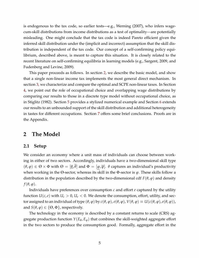
These formulas show that the formula for marginal keep shares 1− T′ is adjusted inthe Pareto problem compared to the SCPE problem by a correction factor that depends onξ and a comparison between the aggregate income share of the Φ-sector, given by
Yϕ(x)Yϕ(x) + xYθ(x)
=Yϕ(x)Eϕ
Yϕ(x)Eϕ + Yθ(x)Eθ=
Yϕ(x)Eϕ
Y(Eθ, Eϕ),
with its local income share y(w) f ϕx (w)/(y(w) fx(w)) = f ϕ
x (w)/ fx(w).8
This is intuitive. For instance, suppose ξ > 0 (we will show below that this corre-sponds to the case where Φ is the low-income sector). Then the marginal keep share isscaled down in the Pareto problem relative to the SCPE whenever, at the given wage (orequivalently income) level, the local income share of the Φ-sector exceeds its aggregateincome share. This disproportionately discourages Φ-sector effort and therefore raiseswages in the Φ-sector relative to the Θ-sector. Hence, the solution to the Pareto problemuses this “indirect redistribution” channel through wages in order to redistribute to thelow-income sector, which is desirable for relative Pareto weights with Ψ(F) ≥ F for allF ∈ [0, 1]. Note that this implies a force towards less progressivity in the Pareto problemrelative to the SCPE: If Φ is the low-income sector, marginal tax rates will be scaled upin the Pareto problem compared to the SCPE for low income levels, and scaled down forhigh income levels.9
Note that, in particular, the top marginal tax rate is not generally zero in a Paretooptimum. It is given by
8It is important, of course, to keep in mind that the formulas in the preceding corollary are evaluatedat endogenously determined values of x. Since, in general, the level of x in the SCPE and the solution tothe Pareto problem will differ for a given economy, the formulas do not permit a direct comparison of taxrates at the two solutions. One interpretation of such a comparison is as a comparison of the tax rates intwo different economies that endogenously happen to have the same skill distribution. By comparing thetax rates with the two formulas, one can infer whether the social planner is solving for an SCPE or a Paretooptimum.
9The same would be true if Φ were the high-income sector. In this case, we will show below that ξ < 0and hence marginal tax rates are again higher in the Pareto optimum compared to the SCPE for low incomelevels, and lower for high income levels, according to (11).
12

Corollary 2. The top marginal tax rate is zero in any SCPE and given by
T′(y(wx)) = ξ(1 + Γ(x))
(f ϕx (wx)
fx(wx)−
Yϕ(x)Yϕ(x) + xYθ(x)
)
in any Pareto optimum. In particular, if f ϕx (wx)/ fx(wx) = 1
(respectively f ϕ
x (wx)/ fx(wx) = 0),
then T′(y(wx)) = ξ (respectively T′(y(wx)) = −ξΓ(x)).
It will turn out below that ξ > 0 if Φ is the low-income sector, and vice versa. But ifΦ is the low-income sector, its local income share at the top of the income distribution issmaller than its aggregate income share, and vice versa. Hence, by Corollary 2, the topmarginal tax rate will generally be negative in a Roy model with regular Pareto weights.For instance, consider the special case of a constant elasticity of substitution (CES) pro-duction function
Y(Eθ, Eϕ) =[αEρ
θ + (1− α)Eρϕ
]1/ρ, (13)
where 1/(1− ρ) is the constant elasticity of substitution. Then the top marginal tax ratein the solution to the Pareto problem simplifies as follows:
Corollary 3. With CES technology, the Pareto optimal top marginal tax rate is
T′(y(wx)) = ξ
(1 +
1− α
αx−ρ
)(f ϕx (wx)
fx(wx)− 1− α
αxρ + 1− α
)
and with Cobb-Douglas technology (ρ = 0),
T′(y(wx)) =ξ
α
(f ϕx (wx)
fx(wx)− (1− α)
).
With Cobb-Douglas technology, the aggregate income share of the Φ-sector is inde-pendent of x and given by the constant 1− α, so that we only need to (i) compare thelocal income (or population) share of the Φ-sector workers among the top wage earnersto 1− α and (ii) determine the sign of the multiplier ξ in order to sign the top marginaltax rate. In order to achieve the second requirement, we consider the outer problem inthe following section.
3.3 Outer Problem
For the following, the substitution elasticity of the production function Y(Eθ, Eϕ), denotedby σ(x), will be useful. The following Lemma provides a simple expression for it.
13

Lemma 3. The substitution elasticity of Y(Eθ, Eϕ) is given by
σ(x) ≡ − 1xλ(x)
with λ(x) ≡Y′θ(x)Yθ(x)
−Y′ϕ(x)Yϕ(x)
.
Proof. See Appendix B.3
Using this, we can derive the following decomposition of the welfare effect of a marginalchange in x.
Lemma 4. For any Pareto weights G, the welfare effect of a marginal change in x can be decom-posed as follows:
W ′(x) = − 1xσ(x)
(I + R + ξµ
[Yϕ(x)Eϕσ(x) + (1 + Γ(x))(S + C)
]), (14)
whereS ≡ 1
Yθ(x)Yϕ(x)
∫ wx
wx
w2e(w) f(
wYθ(x)
,w
Yϕ(x)
)dw > 0, (15)
I ≡ µ∫ wx
wx
η(w)wV′(w)d
dw
(f ϕx (w)
fx(w)
)dw (16)
R ≡∫ wx
wx
wV′(w)f θx (w) f ϕ
x (w)
fx(w)
(gθ
x(w)
f θx (w)
− gϕx (w)
f ϕx (w)
)dw, (17)
and
C ≡∫ wx
wx
w2e′(w)f ϕx (w) f θ
x (w)
fx(w)dw. (18)
Proof. In Appendix B.4.
We provide a heuristic derivation that reveals the intuition behind this result. To thatend, we break the welfare effects of a small change in x into four effects:
1. A direct effect: the effect of changing x on Γ(x) in (5), holding wages and sectors ofeach individual constant.
2. A direct wage shift effect: the effect arising from the change in wages induced by thechange in x, holding each individual’s allocation and sector constant.
3. An indirect wage shift effect: the effect arising from the change in allocations causedby the change in wages induced by the change in x, holding the individual’s sectorconstant.
14

4. A sectoral shift effect: the effect that arises from individuals changing sectors, holdingtheir wages constant.
Notice first that if technology is linear, so that σ(x) = ∞, then setting W ′(x) = 0immediately implies ξ = 0. By Corollary 1, the marginal tax formulas for the SCPEand Pareto problems coincide. This is intuitive: in this case, wages are exogenous tothe tax code, so the fact that there are two sectors is irrelevant. It is only the wage shiftand sectoral shift effects driven by the endogeneity of wages in the finite σ(x) case thatprovide scope for using additional tools for accomplishing redistributive objectives.
Because individual allocations are held constant, the direct wage shift has no effect onthe objective. Because of constant returns to scale, it also has no effect on the resourceconstraint. However, it affects both the incentive and consistency constraints. The ef-fect on the latter can be combined with the direct effect (of changing x on Γ(x)) to yield−Yϕ(x)Eϕ/x. To wit: re-write the consistency condition (5) as Yϕ(x)
(Eθ/x− Eϕ
)= 0,
and consider the effect of a change in x, holding sectors and efforts constant. The termsEθ and Eϕ are unchanged, so the effect is just −Yϕ(x)Eθ/x2 = −Yϕ(x)Eϕ/x.
The term in expression (14) containing I arises from the direct effect of the wage shifton the incentive constraints. To understand it, consider the effects of a small decrease inx for a portion of the wage distribution centered at wage w. Such a decrease will raiseΘ-sector wages and lower Φ-sector wages. If the share of Φ-sector workers is increasinglocally, this leads to a local compression of wage distribution. Such a compression easesthe incentive compatibility constraints if they are binding in the downward direction (i.e.,higher wage individuals need to be prevented from imitating lower wage individuals)—i.e., if η(w) > 0. A decrease in x therefore leads to a welfare improvement insofar asη(w)d
(f ϕx (w)/ fx(w)
)/dw > 0 (and the magnitude of this improvement will be related to
how steeply increasing the utility distribution is). As we will formalize in the subsequentsection, I can be thought of as a (generalized) Stiglitz (1982) effect: with endogenouswages, increasing (decreasing) effort at high (low) wages will raise (lower) wages at low(high) wages.
The sectoral shift and indirect wage-shift effects are effects that are not present inStiglitz’s (1982) framework. It is therefore worth elaborating on why they take the formthey do, and in particular, why they reinforce each other whenever e′(w) > 0. We con-sider the sectoral shift effect first.
15

Δ + Ω Δ
Density: ,
Incomeperindividual:
)
Figure 1: Illustrating the computation of the sectoral shift effect
3.3.1 The sectoral shift
To compute the sectoral shift effect, it is useful to write the consistency condition asΓ(x)Iθ(x) − Iϕ(x) = 0, where Iθ(x) ≡
∫ ww we(w) f θ
x (w)dw is the income earned in theΘ-sector, and similarly for Iϕ(x). Consider a small decrease ∆x in x, holding efforts andwages constant. This will lead some individuals to shift from the Φ- to the Θ-sector, asillustrated in figure 1. Let ∆Iθ(x) denote the resulting change in Θ-sector income. Sincethere is an equal and opposite change in Φ-sector income, the sectoral shift effect can bewritten as
S = (Γ(x) + 1)∆Iθ(x).
Figure 1 illustrates the computation of ∆Iθ(x). It considers the mass element of indi-viduals with Θ-sector skills between θ and θ + dθ who are in the Φ-sector at x but theΘ-sector at x + ∆x. The height of this element is
d(Yθ(x)/Yϕ(x)
)dx
θ∆x =
(Y′θ(x)Yϕ(x)−Yθ(x)Y′ϕ(x)
Yϕ(x)2
)θ∆x.
16

The income earned by each individual in that element is θYθ(x)e (θYθ(x)), and the densityof individuals is f
(θ, θ
Yθ(x)Yϕ(x)
). Multiplying the width (dθ) by the height, the density, and
the per individual income, and then integrating over θ gives:
∆Iθ(x) = ∆x∫ θ
θ
(Y′θ(x)Yϕ(x)−Yθ(x)Y′ϕ(x)
Yϕ(x)2
)Yθ(x)θ2e (θYθ(x)) f
(θ,
θYθ(x)Yϕ(x)
)dθ. (19)
Changing variables to w = θYθ(x) yields,
∆Iθ(x) = ∆xλ(x)
Yθ(x)Yϕ(x)
∫ w
ww2e (w) f
(w
Yθ(x),
wYϕ(x)
)dw. (20)
and the sectoral shift term S defined in expression (15) follows directly.
3.3.2 The indirect wage shift effect
There is no simple graphical representation of the indirect wage shift effect, but a similarheuristic could be used to derive the terms C and R. We omit the algebraic details here,and instead providing the basic intuition behind those effects. (See Appendix B.4 for aformal treatment.)
Imagine increasing x by a small amount while holding the tax code constant so thatallocations e(w) and V(w) are an unchanged function of wages. The two types of indi-viduals at original wage w∗ are affected differently by the change in x: individuals inthe Φ-sector find their (Φ-sector) wage increases; Θ-sector individuals see their wage de-crease. The Θ-sector individuals move down along the (fixed) schedules e(w) and V(w),and Φ-sector individuals move up. Depending on the schedules and the proportions ofthe two types at w∗, the net effort and utility effect on wage w∗-individuals may be posi-tive or negative. The algebraic manipulations in Appendix B.4 are motivated by thinkingof these shifts in two steps: a level shift of all wage w∗-individuals that absorbs the netshift of effort and utility, and a re-allocation of effort and utility across the two types. Theformer involves a particular shift in the e(w) and V(w) schedules, and has zero welfareeffects by an envelope argument (the original schedule was optimal). The re-allocation ofeffort and utility in the latter respectively give rise to the terms C and R in Lemma 4.
Because it arises from a re-allocation of utility across individuals at the same w∗ in-duced by the change in x, the term R disappears when there is no intrinsic sectoralpreference—i.e., when gθ
x(w)/gϕx (w) = f θ
x (w)/ f ϕx (w) for all w. It is straightforward to
show that this will be the case whenever G(θ, ϕ) takes the form G(θ, ϕ) = Ψ(F(θ, ϕ)) orwith relative welfare weights Ψ(Fx(w)). In contrast, when the social planner has an in-
17

trinsic preference for the Θ-sector individuals at wage w∗, the re-allocation of utility fromthe Θ- to the Φ-sector is welfare reducing.
The term C arises from an analogous re-allocation of effort. If the effort schedule isincreasing (i.e. e′(w) ≥ 0), then an increase in x effectively re-allocates effort from theΘ- to the Φ-sector, because Θ-workers move down and Φ-workers up along the e(w)
schedule. This effect therefore reinforces the sectoral shift effect.
3.4 Marginal Tax Rate Results
We can use the decomposition in Lemma 4 to sign the multiplier on the consistency con-dition ξ at an optimal x by setting W ′(x) = 0:
ξ =−(I + R)/σ(x)
Yϕ(x)Eϕ +1 + Γ(x)
σ(x)(C + S)
. (21)
We summarize the resulting conditions for the sign of ξ in the following corollary:
Corollary 4. With linear technology (σ(x) = ∞), ξ = 0.For σ(x) ∈ (0, ∞), the following holds for any Pareto optimum with (i) increasing effort (e′(w) ≥0) and (ii) downwards-binding incentive constraints (η(w) ≥ 0 for all w):
1. ξ ≥ 0 if f θx (w)/ fx(w) is increasing in w and gθ
x(w)/ f θx (w) ≤ gϕ
x (w)/ f ϕx (w) ∀w,
2. ξ ≤ 0 if f ϕx (w)/ fx(w) is increasing in w and gθ
x(w)/ f θx (w) ≥ gϕ
x (w)/ f ϕx (w) ∀w.
The inequalities in (1) and (2) are strict if η(w) is not identically zero.
Conditions (i) and (ii) are sufficient, but not necessary conditions. The former ensuresthat the indirect wage shift term C reinforces the sectoral shift effect. The latter holdswhenever the (average) marginal social value of consumption, given by Uc(w)gx(w)/ fx(w),is decreasing. This is guaranteed with quasilinear-in-consumption preferences and weaklyprogressive welfare weights (such that gx(w)/ fx(w) is increasing), for example. It ensuresthat a compression of the wage distribution eases the incentive compatibility constraints.If f θ
x (w)/ fx(w) is increasing in w, then Θ is the high-skill sector, and an increase in x,by raising wages in the Φ-sector and lowering them in the Θ-sector, has desirable wagecompression effects, as in Stiglitz (1982). This desirable effect is reinforced by R when-ever gϕ
x (w)/ f ϕx (w) ≥ gθ
x(w)/ f θx (w) ∀w. In this case, the social planner puts higher social
welfare weight on Φ-sector workers than on Θ-sector workers at any given wage, and thewage changes induced by an increase in x also have direct benefits.
18

Combining these results from the outer problem with the marginal tax rate resultsfrom the inner problem has crisp implications for the comparison between Pareto op-timal and SCPE tax schedules. For instance, suppose Θ is the high-skilled sector, i.e.f ϕx (w)/ fx(w) is decreasing so that ξ > 0 by Corollary 4. Then the marginal keep share in
the Pareto optimum is scaled down relative to the SCPE if the local income share in theΦ-sector is higher than in aggregate. This disproportionately reduces Φ-sector effort andtherefore indirectly increases wages in the Φ-sector, achieving redistribution to the low-skilled sector. In particular, since f ϕ
x (w)/ fx(w) is decreasing, this means that marginalkeep shares are scaled down for low wages and scaled up for high wages and the topmarginal tax rate is negative.
On the other hand, suppose f ϕx (w)/ fx(w) is increasing, so that ξ < 0. Marginal keep
shares will be scaled down whenever f ϕx (w)/ fx(w) is low, i.e. again for high wages. The
top marginal tax rate is also again negative. I.e. in both of the two cases the general equi-librium effects in the Roy model work in favor of less progressive taxation. We summarizethese insights in the following Proposition:
Proposition 2. If σ(x) ∈ (0, ∞), then the top marginal tax rate is negative in any Pareto opti-mum with
(a) a decreasing i-sector share of workers f ix(w)/ fx(w), i ∈ θ, ϕ,
(b) an increasing effort schedule e(w),
(c) a decreasing social marginal utility of consumption schedule uc(w)gx(w)/ fx(w) and
(d) a weak intrinsic social preference for the i-sector, i.e. gix(w)/ f i
x(w) ≥ gjx(w)/ f j
x(w) for allw, j 6= i ∈ θ, ϕ.
Notably, consider the special case with relative welfare weights Gx(w) = Ψ(Fx(w)).Then gx(w) = ψ(Fx(w)) fx(w) and hence
gθx(w) = ψ(Fx(w)) f θ
x (w) and gϕx (w) = ψ(Fx(w)) f ϕ
x (w).
This immediately implies gθx(w)/ f θ
x (w) = gϕx (w)/ f ϕ
x (w) ∀w and thus R = 0. With rela-tive welfare weights, condition (d) can therefore be dropped.
Hence, these results reveal the following intuitive separation: Per Corollary 4, the signof the multiplier ξ on the consistency constraint accounts for the overall redistributivemotive across sectors, i.e. whether we want to redistribute from Θ to Φ or vice versa.Then conditional on this direction, the nonlinear marginal tax rate correction in the Pareto
19

optimum relative to the SCPE is determined by comparing local and aggregate incomeshares between sectors, per Proposition 1.
4 The Role of Occupational Choice and Continuous Types
In this section, we relate our results to those in Stiglitz (1982), who considers optimalnonlinear taxation in a two-type model with endogenous wages, but without occupa-tional choice. We demonstrate that the general Roy model, with continuous types andoccupational choice, features three extra effects, as captured by S, C and R in the previoussection, that do not appear in any generic discrete type model. The disappearance of thesectoral shift effect S in a model without occupational choice is obvious. In addition, theRoy model with continuous types generates overlapping wage distributions in the twosectors, which gives rise to the effects C and R. In contrast, in a discrete type model, gener-ically – and somewhat unrealistically – there are no workers in different sectors earningthe same wage.
Moreover, we show that the extra “Roy” effects that emerge in our model do notchange the sign of the general equilibrium effects found in Stiglitz (1982), but they miti-gate them. In this sense, redistribution in the Roy model, while implying a less progres-sive optimal tax schedule than a standard Mirrlees model (as captured by a SCPE), leadsto more progressive taxes than a discrete type model without occupational choice.
We start by formulating Stiglitz’s (1982) model in terms of the decomposition into aninner problem (for fixed x) and outer problem (optimizing over x) as so far. Let there betwo types with skills θ and ϕ and with fractions fθ and fϕ = 1− fθ in the population. Weput (relative) Pareto weights ψθ and ψϕ on them such that fθψθ + fϕψϕ = 1. Without lossof generality, we will think of θ as the high wage sector and ϕ as the low wage sector, sothat regular welfare weights satisfy ψθ ≤ 1 and ψϕ ≥ 1. As in Stiglitz (1982), we thereforefocus on the case where only the θ-type’s incentive constraint binds.
4.1 Inner Problem
Individuals are paid their marginal products, wθ = θYθ(x), and wϕ = ϕYϕ(x). Hence, wecan write the inner problem for fixed x as
W(x) = maxeθ ,eϕ,Vθ ,Vϕ
fθψθVθ + fϕψϕVϕ (22)
20

subject to
Vθ ≥ U(
c(cϕ, Vϕ), eϕwϕ
wθ
), (23)
Γ(x) fθwθeθ = fϕwϕeϕ, (24)
fθwθeθ + fϕwϕeϕ ≥ fθc(Vθ, eθ) + fϕc(Vϕ, eϕ
). (25)
As before, the outer problem is just maxx W(x).We focus on the top marginal tax rate and consider the optimal allocation for the θ-
type. Denoting by µ the multiplier on (25) and ξµ on (24), the first order condition w.r.t.eθ is
− fθµ (∂c(Vθ, eθ)/∂eθ − wθ) + fθΓ(x)ξµwθ = 0. (26)
Using ∂c/∂e = −Ue/Uc = MRS, this simplifies to MRSθ = wθ(1 + Γ(x)ξ). By the firstorder condition for the worker’s utility maximization problem, i.e., MRS/w = 1− T′(y),this implies that the marginal tax rate for the high-wage, Θ-sector individual, is −Γ(x)ξas in Corollary 2.
4.2 Outer Problem
We next turn to the outer problem to determine ξ. As before, we can decompose thewelfare effect of a marginal change in x into a direct effect (the derivative with respect tox, holding wages constant), and wage shift effects (from the direct and indirect effects ofchanges in wθ and wϕ). The direct effect is simply
ξµΓ′(x) fθwθeθ = ξµΓ′(x)Yθ(x)Eθ. (27)
We can break the wage shift effects into the effect on the objective and the effects on each ofthe 3 constraints. By the envelope theorem, we can hold Vi and ei, i = θ, ϕ, constant. Thismakes the effect on the objective identically zero. The effect on the resource constraint(25) is also zero, since
fθeθdwθ
dx+ fϕeϕ
dwϕ
dx= EθY′θ(x) + EϕY′ϕ(x) = 0
by constant returns to scale. To compute the effect on (24), re-write the constraint as
Γ(x)(
fθwθeθ + fϕwϕeϕ
)− (1 + Γ(x)) fϕwϕeϕ,
21
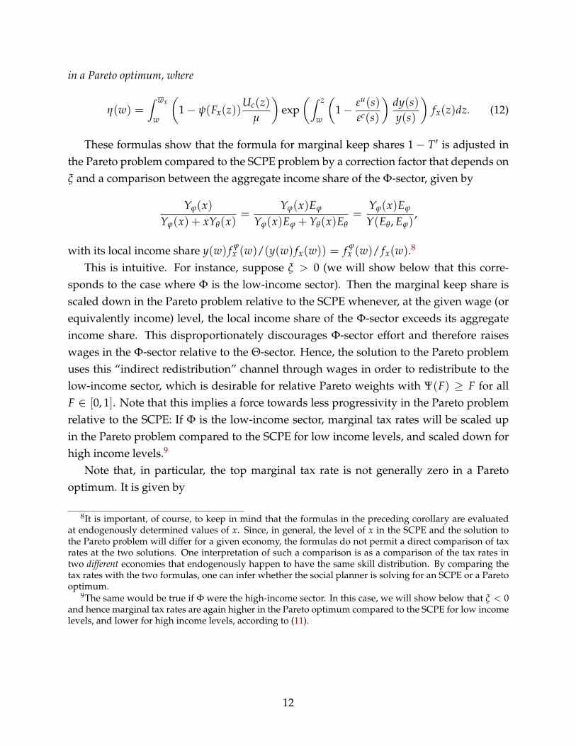
and observe that the derivative of the first term is zero, by the preceding argument.Hence, the effect here is
− ξµ(1 + Γ(x))EϕY′ϕ(x). (28)
Combining (27) and (28) yields −ξµYϕ(x)Eϕ/x just as in section 3.3.Finally, putting a multiplier ηµ on (23), the effect of the wage shift on the incentive
constraint is
−µηUe
(cϕ, eϕ
wϕ
wθ
)eϕ
ϕ
θ
[Y′ϕ(x)Yθ(x)
−Yϕ(x)Y′θ(x)Yθ(x)Yθ(x)
]
= λ(x)µηUe
(cϕ, eϕ
wϕ
wθ
)eϕ
wϕ
wθ≡ λ(x) I. (29)
To see why calling this effect I by analogy to I from the general Roy model is appropriate,consider the definition of I in equation (16) and take the limit where f θ
x (w)/ fx(w) is 0 upuntil wθ, and 1 thereafter. Then the ratio f θ
x (w)/ fx(w) is a step function, the derivative ofwhich is the Dirac δ-function. Hence, the integral in (16) evaluates to −V′(wθ)wθη(wθ) =
Ue(cθ, eθ)eθη(wθ) by the incentive constraint (4). The only difference from I is that it haseϕwϕ/wθ instead of eθ and cϕ rather than cθ (and η is discrete rather than continuous). Thisdifference is a result of the fact that the incentive constraint is discrete rather than local:in the density limit, the θ-type is imitating an infinitesimally close individual, whereas inthe two-type case, the imitation is at a distance. If we let wθ be arbitrarily close to wθ, thenwe would get eθ and cθ, as in the limit case of I.
Combining all of the effects gives
W ′(x) = −ξµYϕ(x)Eϕ/x + λ(x) I
= − 1xσ(x)
[ξµYϕ(x)Eϕ(x)σ(x) + I
].
4.3 Marginal Tax Rates
At an optimum, W ′(x) = 0, so
ξ = − I/σ(x)Yϕ(x)Eϕ
, (30)
which coincides with the general formula (21) if S = C = R = 0 and when we replaceI with I. In particular, the fact that the discrete type model generically rules out twoindividuals with the same wage in different sectors implies C = R = 0. The exogeneity of
22

sectoral allocations eliminates the sectoral shift effect, so S = 0. Moreover, note that thesign of I is opposite of the sign of η. This means that ξ > 0 (and hence top marginal taxesare negative) precisely when we want to redistribute from the θ- to the ϕ-types, so thatthe downward incentive constraint binds.
This is analogous to our results in the general Roy model, but the addition of S andC will make ξ, and hence top marginal taxes, smaller in absolute value. To understandthe intuition behind this, suppose we lower taxes at the top to increase the effort of thetop earners. This is welfare enhancing because it raises the wages of the low wage sectorworkers and lowers the wages of high wage sector workers and thus relaxes the down-ward incentive constraint. However, when there is endogenous occupational choice, thesectoral shift effect works against this, since this change in wages leads some individu-als to shift out of the high wage into the low wage sector, undoing some of the originalincrease in aggregate effort in the high wage sector. The indirect wage shift effect C issimilar: the increase in wages in the low wage sector leads those who do not shift sectorsto work harder, and the decrease in wages in the high wage sector leads those (again, whodo not shift sectors) to work less hard. This also partially offsets the beneficial impact ofincreased effort among high earners.
These additional sectoral shift effects make the regressivity of the tax schedule that isoptimal in the Stiglitz (1982) model less effective. As a result, optimal taxes in the generalRoy model with continuous types, while less progressive than in a standard Mirrleesmodel, are more progressive than in a discrete type model without occupational choice.
5 A Numerical Example
In this section, we briefly illustrate our results with a simple numerical example. Weassume quasilinear preferences U(c, e) = c − h(e) with an isoelastic disutility h(e) =
e1+1/ε/(1 + 1/ε) and an elasticity of labor supply ε = 0.5. The skill distribution hassupport [θ, θ] × [ϕ, ϕ] = [1, 16] × [1, 6] and is independent across the two dimensions,so that F(θ, ϕ) = Fθ(θ)Fϕ(ϕ). We assume that both Fθ and Fϕ are Pareto distributionswith parameters κθ = 2 and κϕ = 8. As a result, there is more mass on lower skillsin the ϕ-dimension compared to θ, and we take Φ as the low skill and Θ as the highskill sector in the following. We truncate both distributions at the top and renormalizeaccordingly. Moreover, to prevent a kink in the wage distribution at ϕ = 6, we shift fϕ sothat fϕ(ϕ) = 0 and renormalize accordingly.
Technology is given by a CES production function as in (13), so that σ = 1/(1− ρ)
is the constant substitution elasticity. In particular, we start with the case ρ = 0 so that
23

0 1 2 3 4 5−0.1
0
0.1
0.2
0.3
0.4
0.5
0.6Marginal Tax Rate
wage0 1 2 3 4 5−0.5
0
0.5
1
1.5
2
2.5Tax Schedule
wage
0 1 2 3 4 5−0.1
0
0.1
0.2
0.3
0.4Average Tax Rate
wage0 1 2 3 4 50
0.2
0.4
0.6
0.8
1Phi−share
wage
OptimumSCPE
Figure 2: Marginal and average tax rates as a function of the wage
the substitution elasticity is one and technology is Cobb-Douglas. We set the aggregateincome share of the high skill sector Θ to α = .2.
Finally, we assume Pareto weights of the form Ψ(F) = 1− (1− F)r. The parameter rthus characterizes the magnitude of the government’s desire for redistribution from highto low wages: With quasilinear preferences, r = 1 implies no redistributive motives, andr → ∞ for a Rawlsian social planner. We take r = 1.3, so that there is some intermediatedesire for redistribution.
Figure 2 shows the marginal tax schedule T′(y(w)), the tax schedule T(y(w)), the av-erage tax rate T(y(w))/y(w) and the share of Φ-sector workers f ϕ
x (w)/ fx(w) as a functionof the wage w both for the Pareto optimum and the SCPE resulting from our parametriza-tion. It illustrates the patterns of the optimal tax policy derived so far: the top marginaltax rate is negative (-9.2%) and the optimal tax schedule is overall less progressive than inthe SCPE. Figure 3 shows the same pattern as a function of income. Since the optimal taxschedule involves lower marginal tax rates at the top, it induces higher effort and hencethe optimal income distribution extends to higher incomes than under the SCPE policy.
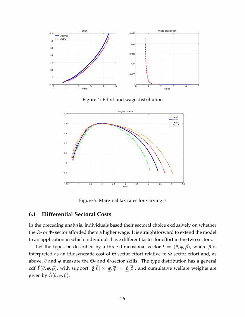
Figure 4 demonstrates that our assumptions are satisfied in the numerical example:individual effort is increasing in the wage w, and the share of Φ-sector workers is mono-
24

0 2 4 6 8 10−0.1
0
0.1
0.2
0.3
0.4
0.5
0.6Marginal Tax Rate
income
0 2 4 6 8 10−0.5
0
0.5
1
1.5
2
2.5Tax Schedule
income
0 2 4 6 8 10−0.1
0
0.1
0.2
0.3
0.4Average Tax Rate
income0 2 4 6 8 100
0.2
0.4
0.6
0.8
1Phi−share
income
OptimalSCPE
Figure 3: Marginal and average tax rates as a function of income
tone. A fortiori, income y(w) = we(w) is increasing in the wage, so that bunching doesnot need to be considered.
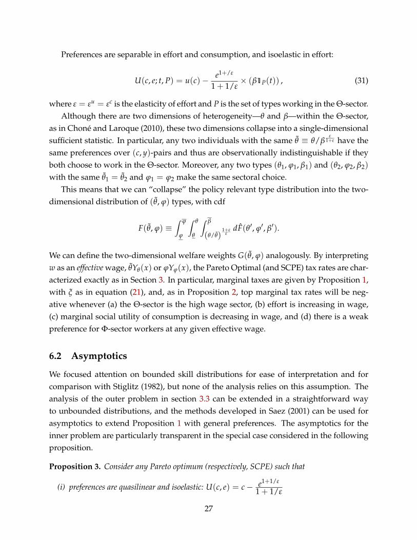
In figure 5, we plot the marginal tax schedule for varying substitution elasticities σ ∈2, 1, 0.5, 0.1. It shows that the tax schedule becomes less and less progressive as wemove to lower substitution elasticities. This is because the general equilibrium effectsfrom the endogeneity of wages become more pronounced as we move away from lineartechnology, with σ = ∞ and ρ = 1. As a result, the corresponding top marginal tax ratesbecome more negative, moving from -7.6% to -9.2%, -10.8% and -11.9%.
6 Extensions
We consider two extensions here: allowing individuals to face different costs of workingin different sectors, and an extension to unbounded skill distributions.
25
0 1 2 3 4 50.8
1
1.2
1.4
1.6
1.8
2
2.2Effort
wage
0 1 2 3 4 50
0.005
0.01
0.015
0.02
0.025Wage distribution
wage
OptimalSCPE
Figure 4: Effort and wage distribution
0.5 1 1.5 2 2.5 3 3.5 4 4.5 5 5.5−0.2
−0.1
0
0.1
0.2
0.3
0.4
0.5Marginal Tax Rate
wage
rho=.5rho=0rho=−1rho=−9
Figure 5: Marginal tax rates for varying σ
6.1 Differential Sectoral Costs
In the preceding analysis, individuals based their sectoral choice exclusively on whetherthe Θ- or Φ- sector afforded them a higher wage. It is straightforward to extend the modelto an application in which individuals have different tastes for effort in the two sectors.
Let the types be described by a three-dimensional vector t = (θ, ϕ, β), where β isinterpreted as an idiosyncratic cost of Θ-sector effort relative to Φ-sector effort and, asabove, θ and ϕ measure the Θ- and Φ-sector skills. The type distribution has a generalcdf F(θ, ϕ, β), with support [θ, θ] × [ϕ, ϕ] × [β, β], and cumulative welfare weights aregiven by G(θ, ϕ, β).
26
Preferences are separable in effort and consumption, and isoelastic in effort:
U(c, e; t, P) = u(c)− e1+/ε
1 + 1/ε× (β1P(t)) , (31)
where ε = εu = εc is the elasticity of effort and P is the set of types working in the Θ-sector.Although there are two dimensions of heterogeneity—θ and β—within the Θ-sector,
as in Choné and Laroque (2010), these two dimensions collapse into a single-dimensionalsufficient statistic. In particular, any two individuals with the same θ ≡ θ/β
ε1+ε have the
same preferences over (c, y)-pairs and thus are observationally indistinguishable if theyboth choose to work in the Θ-sector. Moreover, any two types (θ1, ϕ1, β1) and (θ2, ϕ2, β2)
with the same θ1 = θ2 and ϕ1 = ϕ2 make the same sectoral choice.This means that we can “collapse” the policy relevant type distribution into the two-
dimensional distribution of (θ, ϕ) types, with cdf
F(θ, ϕ) ≡∫ ϕ
ϕ
∫ θ
θ
∫ β
(θ/θ)1+ε
εdF(θ′, ϕ′, β′).
We can define the two-dimensional welfare weights G(θ, ϕ) analogously. By interpretingw as an effective wage, θYθ(x) or ϕYϕ(x), the Pareto Optimal (and SCPE) tax rates are char-acterized exactly as in Section 3. In particular, marginal taxes are given by Proposition 1,with ξ as in equation (21), and, as in Proposition 2, top marginal tax rates will be neg-ative whenever (a) the Θ-sector is the high wage sector, (b) effort is increasing in wage,(c) marginal social utility of consumption is decreasing in wage, and (d) there is a weakpreference for Φ-sector workers at any given effective wage.
6.2 Asymptotics
We focused attention on bounded skill distributions for ease of interpretation and forcomparison with Stiglitz (1982), but none of the analysis relies on this assumption. Theanalysis of the outer problem in section 3.3 can be extended in a straightforward wayto unbounded distributions, and the methods developed in Saez (2001) can be used forasymptotics to extend Proposition 1 with general preferences. The asymptotics for theinner problem are particularly transparent in the special case considered in the followingproposition.
Proposition 3. Consider any Pareto optimum (respectively, SCPE) such that
(i) preferences are quasilinear and isoelastic: U(c, e) = c− e1+1/ε
1 + 1/ε
27

(ii) the top earners are all in the Θ-sector: limw→∞f ϕx (w)fx(w)
= 0
(iii) the Θ-sector skill distribution has Pareto tails with parameter κ: limw→∞1− Fx(w)
w fx(w)= κ
(iv) Pareto weights are relative and progressive: Gx(w) = Ψ(Fx(w)) with Ψ′′(x) < 0 and
(vi) zero welfare weight is put on the top earners: Ψ′(1) = 0.
Then the top marginal tax rate is
κ (1 + 1/ε)− ξΓ(x)κ (1 + 1/ε) + 1
(respectively,
κ (1 + 1/ε)
κ (1 + 1/ε) + 1
), (32)
and ξ > 0.
Proof. In Appendix B.5
In particular, this implies that asymptotic taxes are scaled down in the Pareto optimumrelative to the SCPE.
7 Conclusion
We view this paper as making a two-fold contribution. The first is methodological: weprovide a technique for solving a multi-dimensional screening problem in an importantclass of contexts. Specifically, we show that the multi-dimensional screening problemthat arises in designing optimal taxation in a multiple-sector economy can be reduced toa single dimensional optimal income tax problem à la Mirrlees. This basic technique islikely to be applicable more broadly.
Our second contribution is to derive some of the implications that self-selection intooccupational sectors can have for optimal income taxation. In particular, we show thatthe presence of several complementary sectors in an economy provides a force pushingtowards less progressive taxation.
Central to this result is our assumption—we believe quite reasonable—that the gov-ernment cannot or chooses not to observe the sector an individual is employed in when itlevies taxes. In ongoing research, we aim at relaxing this assumption and characterizingoptimal sector-specific taxation.
28

References
ALLEN, F. (1982): “Optimal Linear Income Taxation with General Equilibrium Effects onWages,” Journal of Public Economics, 17, 135–143.
BOADWAY, R., N. MARCEAU, AND P. PESTIEAU (1991): “Optimal Linear Income Taxationin Models with Occupational Choice,” Journal of Public Economics, 46, 133–162.
BORJAS, G. (1987): “Self-Selection and the Earnings of Immigrants,” American EconomicReview, 77, 531–553.
(2002): “The Wage Structure and the Sorting of Workers into the Public Sector,”NBER Working Paper 9313.
CHONÉ, P., AND G. LAROQUE (2010): “Negative Marginal Tax Rates and Heterogeneity,”American Economic Review, 100, 2532–2547.
DIAMOND, P. (1998): “Optimal Income Taxation: An Example with a U-shaped Patternof Optimal Tax Rates,” American Economic Review, 88, 83–95.
FELDSTEIN, M. (1973): “On the Optimal Progressivity of the Income Tax,” Journal of PublicEconomics, 2, 356–376.
FUDENBERG, D., AND D. LEVINE (2009): “Self-confirming equilibrium and the Lucas cri-tique,” Journal of Economic Theory, 144, 2354–2371.
KLEVEN, H. J., C. T. KREINER, AND E. SAEZ (2009): “The Optimal Income Taxation ofCouples,” Econometrica, 77, 537–560.
LAROQUE, G. (2005): “Income maintenance and labor force participation,” Econometrica,73, 341–376.
MIRRLEES, J. (1971): “An Exploration in the Theory of Optimum Income Taxation,” Re-view of Economic Studies, 38, 175–208.
MORESI, S. (1997): “Optimal Taxation and Firm Formation: A Model of AsymmetricInformation,” European Economic Review, 42, 1525–1551.
NAITO, H. (1999): “Re-Examination of Uniform Commodity Taxes Under A Non-LinearIncome Tax System And Its Implication for Production Efficiency,” Journal of PublicEconomics, 71, 165–188.
29

PARKER, S. C. (1999): “The Optimal Linear Taxation of Employment and Self-Employment Incomes,” Journal of Public Economics, 73, 107–123.
ROCHET, J.-C., AND P. CHONÉ (1998): “Ironing, Sweeping and Multidimensional Screen-ing,” Econometrica, 66, 783–826.
ROTHSCHILD, C., AND F. SCHEUER (2011): “Optimal Taxation with Rent-Seeking,” NBERWorking Paper 17035.
ROY, A. (1951): “Some Thoughts on the Distribution of Earnings,” Oxford Economic Papers,3, 135–146.
SAEZ, E. (2001): “Using Elasticities to Derive Optimal Tax Rates,” Review of EconomicStudies, 68, 205–229.
SARGENT, T. (2008): “Evolution and Intelligent Design,” American Economic Review, 98,5–37.
STIGLITZ, J. (1982): “Self-Selection and Pareto Efficient Taxation,” Journal of Public Eco-nomics, 17, 213–240.
WERNING, I. (2007): “Pareto-Efficient Income Taxation,” Mimeo, MIT.
ZECKHAUSER, R. (1977): “Taxes in Fantasy, or Most Any Tax on Labor Can Turn Out toHelp the Laborers,” Journal of Public Economics, 8, 133–150.
A Proofs for Section 2
A.1 Proof of Lemma 1
We prove the result in the following four steps:Step 1. It is an immediate consequence of the incentive constraints that the utility of a type sent to a
given sector can only depend on his wage in that sector. Formally, consider two types (θ0, ϕ0) and (θ1, ϕ1)
withS(θ0, ϕ0) = S(θ1, ϕ1) = Θ and Yθ(x)θ0 = Yθ(x)θ1 = w.
Whenever
U(
c(w/Yθ(x), ϕ0),y(w/Yθ(x), ϕ0)
w
)6= U
(c(w/Yθ(x), ϕ1),
y(w/Yθ(x), ϕ1)
w
),
either type (w/Yθ(x), ϕ0)’s or type (w/Yθ(x), ϕ1)’s incentive constraint is violated. An analogous argumentapplies to types sent to the Φ-sector. Since w is the wage of the agent in the sector that he is sent to, we canthus write utilities as Vθ(w) for all types for which S(θ, ϕ) = Θ and Vϕ(w) for all types with S(θ, ϕ) = Φ.
30

Step 2. We now show that the consumption and income allocated to a type who is sent to a given sectorcan also only depend on his skill in that sector. To see this, consider again two types (θ0, ϕ0) and (θ1, ϕ1)
withS(θ0, ϕ0) = S(θ1, ϕ1) = Θ and θ0 = θ1 = w/Yθ(x).
Consider the expression
H(w, w′) =
[U(
c(w′/Yθ(x), ϕ0),y(w′/Yθ(x), ϕ0)
w′
)−U
(c(w/Yθ(x), ϕ0),
y(w/Yθ(x), ϕ0)
w′
)]−[
U(
c(w′/Yθ(x), ϕ1),y(w′/Yθ(x), ϕ1)
w′
)−U
(c(w/Yθ(x), ϕ1),
y(w/Yθ(x), ϕ1)
w′
)].
Mechanically, we have∂H(w, w′)
∂w′
∣∣∣∣w′=w
= 0,
since the partial derivative of each bracketed term, evaluated at w′ = w, is individually zero. On the otherhand, we showed in 1. that
U(
c(w′/Yθ(x), ϕ0),y(w′/Yθ(x), ϕ0)
w′
)= U
(c(w′/Yθ(x), ϕ1),
y(w′/Yθ(x), ϕ1)
w′
)= Vθ(w′),
so that H(w, w′) reduces to
H(w, w′) = U(
c(w/Yθ(x), ϕ1),y(w/Yθ(x), ϕ1)
w′
)−U
(c(w/Yθ(x), ϕ0),
y(w/Yθ(x), ϕ0)
w′
).
Single-crossing implies that
Uw
(c(w/Yθ(x), ϕ1),
y(w/Yθ(x), ϕ1)
w
)≷ Uw
(c(w/Yθ(x), ϕ0),
y(w/Yθ(x), ϕ0)
w
)whenever
U(
c(w/Yθ(x), ϕ1),y(w/Yθ(x), ϕ1)
w
)= U
(c(w/Yθ(x), ϕ0),
y(w/Yθ(x), ϕ0)
w
)and c(w/Yθ(x), ϕ1) ≷ c(w/Yθ(x), ϕ0).10 Hence, it must be that
c(w/Yθ(x), ϕ1) = c(w/Yθ(x), ϕ0) and y(w/Yθ(x), ϕ1) = y(w/Yθ(x), ϕ0).
The same argument applies to types sent to the Φ-sector. We can thus write allocations as cθ(w), yθ(w) forall types with S(θ, ϕ) = Θ and cϕ(w), yϕ(w) for all types with S(θ, ϕ) = Φ.
Step 3. It is also straightforward to see that two types who earn the same wage in different sectors mustget the same utility. Consider two types (θ0, ϕ0) and (θ1, ϕ1) with
S(θ0, ϕ0) = Θ, S(θ1, ϕ1) = Φ and Yθ(x)θ0 = Yϕ(x)ϕ1 = w.
10Recall that single crossing implies that −Ue/(wUc) is decreasing in w, or equivalently that Uy/Uc isincreasing in w and hence UywUc −UyUcw > 0. Therefore, the change in Uw from a marginal increase in cand y along w’s indifference curve (i.e. such that dc = −(Uy/Uc)dy) is dUw = Uwy − (Uy/Uc)Uwc > 0.
31

Next, assume w.l.o.g.
U(
cθ(w),yθ(w)
w
)> U
(cϕ(w),
yϕ(w)
w
).
Then the (θ1, w/Yϕ(x))-type could imitate the (w/Yθ(x), ϕ0)-type by producing income yθ(w) but doing soin the Φ-sector, i.e. using his skill w/Yϕ(x). His utility from this deviation would be exactly the LHS of theabove inequality, contradicting incentive compatibility. This shows
Vθ(w) = Vϕ(w) ≡ V(w) ∀w.
Step 4. We finally show that the incentive constraints also imply that allocations have to be such that
cθ(w) = cϕ(w) ≡ c(w) and yθ(w) = yϕ(w) ≡ y(w) ∀w,
i.e. two types who earn the same wage in different sectors must get the same consumption and income. Forthis purpose, consider again the expression
H(w, w′) =
[U(
cθ(w′),yθ(w′)
w′
)−U
(cθ(w),
yθ(w)
w′
)]−[
U(
cϕ(w′),yϕ(w′)
w′
)−U
(cϕ(w),
yϕ(w)
w′
)].
Now consider again ∂H/∂w′|w′=w. On the one hand, this is mechanically zero since the partial derivativeof each bracketed term is individually zero. On the other hand,
U(
cθ(w′),yθ(w′)
w′
)= U
(cϕ(w′),
yϕ(w′)w′
)by step 3., so
H(w, w′) = U(
cϕ(w),yϕ(w)
w′
)−U
(cθ(w),
yθ(w)
w′
),
and, by single crossing
Uw
(cϕ(w),
yϕ(w)
w
)≷ Uw
(cθ(w),
yθ(w)
w
)whenever U(cϕ(w), yϕ(w)/w) = U(cθ(w), yθ(w)/w) and cϕ(w) ≷ cθ(w). Hence, it must be that cϕ(w) =
cθ(w) and yϕ(w) = yθ(w) for all w.These four steps prove that any incentive compatible direct mechanism in our economy can be imple-
mented by offering a schedule of c(w), y(w) bundles with w ≡ maxYθ(x)θ, Yϕ(x)ϕ, which is equivalentto a single non-linear tax schedule.
32

B Proofs for Section 3
B.1 Proof of Lemma 2By changing variables to p ≡ Fx(w), we can write the planner’s welfare in any feasible allocation as
SW =∫ wx
wx
ψ(Fx(w))V(w)dFx(w) =∫ 1
0ψ(p)V
(F−1
x (p))
dp
with ψ(F) = Ψ′(F). Note that the welfare weights ψ(p) are independent of the allocation and that SWdepends only on the distribution of V in this formulation. It follows that if the distribution of V underone feasible allocation first order stochastically dominates (FOSD) the distribution of V under a secondfeasible allocation, then social welfare is higher under the first allocation. To complete the proof, notethat x0, e0(θ, ϕ), V0(θ, ϕ) cannot maximize social welfare if it is Pareto dominated by a feasible allocationx1, e1(θ, ϕ), V1(θ, ϕ), as the distribution of V1 would then FOSD the distribution of V0.
B.2 Proof of Proposition 1Putting multipliers µ on (6), ξλ on (5) and η(w)µ on (4), the Lagrangian corresponding to (3)-(6) is, afterintegrating by parts (4),
L =∫ wx
wxV(w)gx(w)dw−
∫ wxwx
V(w)η′(w)µdw +∫ wx
wxUe(c(V(w), e(w)), e(w)) e(w)
w η(w)µdw
+ξµΓ(x)∫ wx
wxwe(w) f θ
x (w)dw− ξµ∫ wx
wxwe(w) f ϕ
x (w)dw
+µ∫ wx
wxwe(w) fx(w)dw− µ
∫ wxwx
c(V(w), e(w)) fx(w)dw. (33)
Using ∂c/∂V = 1/Uc and compressing notation, the first order condition for V(w) is
η′(w)µ = gx(w)− µ fx(w)1
Uc(w)+ η(w)µ
Uec(w)
Uc(w)
e(w)
w. (34)
Defining η(w) ≡ η(w)Uc(w), this becomes
η′(w) = gx(w)Uc(w)
µ− fx(w) + η(w)
Ucc(w)c′(w) + Uce(w)e′(w) + Uce(w)e(w)/wUc(w)
. (35)
Using the first order condition corresponding to the optimization problem for an individual worker,
Uc(w)c′(w) + Ue(w)e′(w) + Ue(w)e(w)
w= 0,
the fraction in (35) can be written as −(∂MRS(w)/∂c)y′(w)/w where
MRS(w) ≡ −Ue(c(w), e(w))
Uc(c(w), e(w))
33

is the marginal rate of substitution between effort and consumption. Substituting in (35) and rearrangingyields
− ∂MRS(w)
∂ce(w)
y′(w)
y(w)η(w) = fE(w)− ψE(w)
Uc(w)
µ+ η′(w). (36)
Integrating this ODE gives
η(w) =∫ wx
w
(fx(w)− ψx(z)
Uc(z)µ
)exp
(∫ z
w
∂MRS(s)∂c
e(s)y′(s)y(s)
ds)
dz
=∫ wx
w
(1− ψx(z)
fx(z)Uc(z)
µ
)exp
(∫ z
w
(1− εu(s)
εc(s)
)dy(s)y(s)
)fx(z)dz, (37)
where the last step follows from e(w)∂MRS(w)/∂c = 1− εu(w)/εc(w) after tedious algebra (e.g. usingequations (23) and (24) in Saez, 2001).
Using ∂c/∂e = MRS, the first order condition for e(w) is
µw fx(w)
(1− MRS(w)
w
)− ξµw
(Γ(x) f θ
x (w)− f ϕx (w)
)= −η(w)µ
[(−Uec(w)Ue(w)/Uc(w) + Uee(w)) e(w)
w+
Ue(w)
w
],
which after some algebra can be rewritten as
w fx(w)
(1− MRS(w)
w
)+ ξw
(Γ(x) f θ
x (w)− f ϕx (w)
)= η(w)
(∂MRS(w)
∂eew
+MRS(w)
w
). (38)
Noting that MRS(w)/w = 1− T′(y(w)) from the first order condition of the workers’ utility maximizationproblem and using the definition of η(w), this becomes
1 + ξΓ(x) f θ
x (w)− f ϕx (w)
fx(w)= (1− T′(y(w)))
[1 +
η(w)
w fx(w)
(1 +
∂MRS(w)
∂ee
MRS(w)
)]. (39)
Simple algebra again shows that 1 + ∂ log MRS(w)/∂ log e = (1 + εu(w))/εc(w), and that
Γ(x) f θx (w)− f ϕ
x (w)
fx(w)=
Yϕ(x)Yϕ(x) + xYθ(x)
− f ϕx (w)
fx(w).
The Proposition follows from (37) and (39).
B.3 Proof of Lemma 3The substitution elasticity is defined as
σ(x) ≡ dxx
Yϕ(x)/Yθ(x)d(Yϕ(x)/Yθ(x)
) =1
d(Yϕ(x)/Yθ(x)
)dx
Yϕ(x)xYθ(x)
=Yθ(x)Yϕ(x)
x1
Yθ(x)Y′ϕ(x)−Yϕ(x)Y′θ(x)=
1
xY′ϕ(x)Yϕ(x)
− xY′θ(x)Yθ(x)
= − 1xλ(x)
.
34

B.4 Proof of Lemma 4We first state the following technical lemma—the proof of which involves nothing more than tedious alge-bra.
Lemma 5.
dFθx (w)
dx= −
Y′θ(x)Yθ(x)
w f θx (w) + Ωx(w) and
dFϕx (w)
dx= −
Y′ϕ(x)Yϕ(x)
w f ϕx (w)−Ωx(w)
with
Ωx(w) ≡ 1Yθ(x)Yϕ(x)
λ(x)∫ w
wx
w′ f(
w′
Yθ(x),
w′
Yϕ(x)
)dw′.
Completely analogous expressions hold for Gθx(w) and Gϕ
x (w).
This will be useful in the proof of Lemma 4, to which we now turn. Using (33),
W ′(x) =∫ wx
wx
V(w)dgx(w)
dxdw− µ
∫ wx
wx
c(V(w), e(w))d fx(w)
dxdw + ξµΓ′(x)Yθ(x)Eθ
+ µξ
(Γ(x)
∫ wx
wx
we(w)d f θ
x (w)
dxdw−
∫ wx
wx
we(w)d f ϕ
x (w)
dxdw
)+ µ
∫ wx
wx
we(w)d fx(w)
dxdw + B1
with
B1 ≡dwx
dx
[V(wx)gx(wx)− µc(V(wx), e(wx)) fx(wx) + µ
(fx(wx) + ξ
(Γ(x) f θ
x (e(wx))− f ϕx (e(wx))
))wxe(wx)
]−dwx
dx
[V(wx)gx(wx)− µc(V(wx), e(wx)) fE(wx) + µ
(fx(wx) + ξ
(Γ(x) f θ
x (e(wx))− f ϕx (e(wx))
))wxe(wx)
].
Integrating by parts the five integral terms yields
W ′(x) = B1 + B2 −∫ wx
wx
V′(w)dGx(w)
dxdw + µ
∫ wx
wx
(V′(w)
Uc(w)+ MRS(w)e′(w)
)dFx(w)
dxdw + ξµΓ′(x)Yθ(x)Eθ
+µξ
(∫ wx
wx
(we′(w) + e(w))
(dFϕ
x (w)
dx− Γ(x)
dFθx (w)
dx
)dw
)− µ
∫ wx
wx
(we′(w) + e(w))dFx(w)
dxdw
(40)
with
B2 =
[V(w)
dGx(w)
dx− µc(V(w), e(w))
dFx(w)
dx+ µξwe(w)
(Γ(x)
dFθx (w)
dx− dFϕ
x (w)
dx
)+ µwe(w)
dFx(w)
dx
]wx
wx
.
By the first order conditions (36) and (38) with respect to V(w) and e(w) from the inner problem, the terms
µ∫ wx
wx
e′(w)
fx(w)
[w fx(w)
(1− MRS(w)
w
)+ ξw
(Γ(x) f θ
x − f ϕx (w)
)− η(w)
(∂MRS(w)
∂ee(w)
w+
MRS(w)
w
)]dFx(w)
dxdw
and
µ∫ wx
wx
V′(w)
Uc(w) fx(w)
[gx(w)
Uc(w)
λ− fx(w)− η′(w)− η(w)
∂MRS(w)
∂ce(w)
y′(w)
y(w)
]dFx(w)
dxdw
35

are both equal to zero. Adding them to (40), using (4) and re-arranging yields
W ′(x) = B1 + B2 + ξµΓ′(x)Yθ(x)Eθ +∫ wx
wx
V′(w)
(gx(w)
fx(w)
dFx(w)
dx− dGx(w)
dx
)dw
− µ∫ wx
wx
e(w)dFx(w)
dxdw− µ
∫ wx
wx
(η(w)
wd [MRS(w)e(w)]
dw+ η′(w)
V′(w)
Uc(w)
)1
fx(w)
dFx(w)
dxdw
+ ξµ∫ wx
wx
((e(w) + we′(w))
(dFϕ
x (w)
dx− Γ(x)
dFθx (w)
dx
)+ we′(w)
(Γ(x)
f θx (w)
fx(w)− f ϕ
x (w)
fx(w)
)dFx(w)
dx
)dw.
(41)
From Lemma 5,
gx(w)
fx(w)
dFx(w)
dx− dGx(w)
dx= −
Y′θ(x)Yθ(x)
[gx(w)
fx(w)f θx (w)− gθ
x(w)
]+
Y′ϕ(x)Yϕ(x)
[gx(w)
fx(w)f ϕx (w)− gϕ
x (w).]
=
(Y′θ(x)Yθ(x)
−Y′ϕ(x)Yϕ(x)
)[gx(w)
fx(w)f ϕx (w)− gϕ
x (w)
]
= λ(x)f ϕx (w) f θ
x (w)
fx(w)
(gθ
x(w)
f θx (w)
− gϕx (w)
f ϕx (w)
).
The first integral in (41) is therefore
∫ wx
wx
V′(w)
(gx(w)
fx(w)
dFx(w)
dx− dGx(w)
dx
)dw = λ(x)R (42)
Combining the terms with e(w) on the second and third line of (41) and using lemma 5 and the identityY′θ(x)Eθ + Y′ϕ(x)Eϕ ≡ 0 gives:
−µ∫ wx
wx
e(w)dFx(w)
dxdw + ξµ
∫ wx
wx
e(w)
(dFϕ
x (w)
dx− Γ(x)
dFθx (w)
dx
)dw
= µ
[Y′θ(x)Yθ(x)
∫ wx
wx
we(w) f θx (w)dw +
Y′ϕ(x)Yϕ(x)
∫ wx
wx
we(w) f ϕx (w)dw
]
+ ξµ∫ wx
wx
we(w)
(Γ(x)
Y′θ(x)Yθ(x)
f θx (w)−
Y′ϕ(x)Yϕ(x)
f ϕx (w)
)dw− ξµ(1 + Γ(x))
∫ wx
wx
e(w)Ωx(w)dw
= 0 + ξµ (1 + Γ(x))Y′θEθ − ξµ(1 + Γ(x))∫ wx
wx
e(w)Ωx(w)dw. (43)
36

The terms with we′(w) in the last line (41) can be written, using Lemma 5 again, as
ξµ∫ wx
wx
we′(w)
(dFϕ
x (w)
dx− Γ(x)
dFθx (w)
dx
)+ we′(w)
(Γ(x)
f θx (w)
fx(w)− f ϕ
x (w)
fx(w)
)dFx(w)
dx
= ξµ∫ wx
wx
w2e′(w)
[Γ(x)
Y′θ(x)Yθ(x)
f θx (w)−
Y′ϕ(x)Yϕ(x)
f ϕx (x)−
(Γ(x)
f θx (w)
fx(w)− f ϕ
x (w)
fx(w)
)(Y′θ(x)Yθ(x)
f θx (w) +
Y′ϕ(x)Yϕ(x)
f ϕx (x)
)]dw
− ξµ(1 + Γ(x))∫ wx
wx
we′(w)Ωx(w)dw
= λ(x)ξµ(1 + Γ(x))C− ξµ(1 + Γ(x))∫ wx
wx
we′(w)Ωx(w)dw, (44)
where the first term in the last step follows after some tedious algebra.Combining the terms with Ωx(w) from (43) and (44) gives−ξµ(1+ Γ(x))
∫ wxwx
(we(w))′Ωx(w)dw, whichcan be integrated by parts to yield:
− B3 + (1 + Γ(x))ξµλ(x)
Yθ(x)Yϕ(x)
∫ wx
wx
w2e(w) f(
wYθ(x)
,w
Yϕ(x)
)dw = (1 + Γ(x))ξµλ(x)S, (45)
with B3 = (1 + Γ(x))ξµwxe(wx)Ωx(wx) since Ωx(wx) = 0.Finally, use the incentive constraint (4), rewritten as V′(w)/Uc(w) = MRS(w)e(w), to write the last line
of (41) as
−λ∫ wx
wx
(η(w)w
d[V′(w)/Uc(w)]
dw+ η′(w)w
V′(w)
Uc(w)+ η(w)
V′(w)
Uc(w)
)1
w fx(w)
dFx(w)
dxdw
or, recognizing the sum of the bracketed terms as d[η(w)wV′(w)/Uc(w)]/dw, integrating by parts, andusing the transversality condition η(wx) = η(wx) = 0 and Lemma 5,
µ∫ wx
wx
η(w)wV′(w)d
dw
(−(
Y′θ(x)Yθ(x)
f θx (w)
fx(w)−
Y′ϕ(x)Yϕ(x)
f ϕx (w)
fx(w)
))dw = µλ(x)I (46)
Define F(w, x) ≡ Fx(w). Since F(wx, x) ≡ 1 for all x,
dF(wx, x)dx
=∂F(wx, x)
∂x+
∂F(wx, x)∂w
dwx
dx=
dFx(wx)
dx+ fx(wx)
dwx
dx= 0. (47)
Together with an analogous expression at wx, the fact that Ωx(wx) = 0, and Lemma 5, this yields
B1 + B2 = −ξµwxe(wx)Ωx(wx) = B3.
Using (42), (43), (44), (45) and (46) in (41) yields
W ′(E) = λ(x)(
I + R + ξµ[Yϕ(x)Eϕσ(x) + (1 + Γ(x))(S + C)
]), (48)
where we have used(Γ′(x)Yθ(x) + (1 + Γ(x))Y′θ(x)
)Eθ = −Yϕ(x)Eϕ/x.
37

B.5 Proof of Proposition 3
limw→∞
1− T′(y(w)) = limw→∞
1 + ξ(1 + Γ(x))
(Yϕ(x)
Yϕ(x) + xYθ(x)− f ϕ
x (w)
fx(w)
)
1 +η(w)
w fx(w)
1 + εu(w)
εc(w)
=
1 + ξ(1 + Γ(x))
(Yϕ(x)
Yϕ(x) + xYθ(x)− lim
w→∞
(f ϕx (w)
fx(w)
))
1 +(
1 +1ε
)lim
w→∞
(1− Fx(w)
w fx(w)
)(Ψ(Fx(w))− Fx(w)
1− Fx(w)
)
=
1 + ξ(1 + Γ(x))(
Yϕ(x)Yϕ(x) + xYθ(x)
)1 +
(1 +
1ε
)κ
=1 + ξΓ(x)
1 +(
1 +1ε
)κ
.
The first equality is from (11). The second uses (iv) and (i), which implies η(w) = Ψ(Fx(w))− Fx(w). Thethird line uses (ii) to simplify the numerator, and (iii) and (v) to take the limits of the two terms in thedenominator. The final step is simple algebra. The top tax rate result for the Pareto optimum follows witha little re-arranging. Setting ξ = 0 yields the result for the SCPE. Corollary 4 and (iv) imply ξ > 0, sinceΨ′′(x) < 0 implies that gx(w)/ fx(w) = Ψ′(Fx(w)) is decreasing in w.
38