Embed Size (px)
Citation preview
Postadress: Besöksadress: Telefon:
Box 1026 Gjuterigatan 5 036-10 10 00 (vx)
551 11 Jönköping
REDESIGN OF A SHOCK ABSORBER
PISTON USING SINTERING
Ömer Kus
Hamed Mojtabavi
EXAM WORK 2012
MECHANICAL ENGINEERING
Postadress: Besöksadress: Telefon:
Box 1026 Gjuterigatan 5 036-10 10 00 (vx)
551 11 Jönköping
This exam work has been carried out at the School of Engineering in
Jönköping in the subject area Mechanical Engineering. The work is a part of
the Master of Science programme.
The authors take full responsibility for opinions, conclusions and findings
presented.
Examiner: Roland Stolt
Supervisor: Roland Stolt
Scope: 30 credits
Date: 12.06.2012
Abstract
1
Abstract
The main objective of this report is to re-design of a product by substituting for another manufacturing process in order to get a cheaper product with the same function and quality. The current shock absorber piston is manufactured by the machining process at Öhlins Racing AB Company. Power Metallurgy (P/M) method could be a good substitute process to meet the technical requirements of the current piston with total lower cost. In this case, the whole process of product development gets involved in designing two new pistons from base-design to final product. One design is assigned to a cheaper P/M process as called Conventional Press and Sinter. Another P/M process as called Metal Injection Molding (MIM) is considered to produce the more expensive piston. According to the design guidelines of P/M processes, the base pistons are modelled in a three dimensional environment, and then an appropriate powder metal is selected for each. Consequently, the next stage is to analyse the piston strengths by Finite Element Method under the static and dynamic loadings. Fatigue analysis is taken into consideration for the cyclic loadings, and the static strength can be assessed for the static loading mode. The results show the infinite fatigue life for two different designs, and no plastic deformation is observed during analysing of the pistons under static loading. Cost estimation is the last stage of this master thesis. Compared to the total costs for the current design, the total estimations for the whole final P/M products can prove the significant drop in the final prise for each design. Thus, environmental and financial issues are already met in achieving the new pistons in this project by saving considerably money and energy. On-going stages will be to make prototype and get them tested under the real working conditions in respect to the standards.

Keywords
2
Keywords
P/M (Power Metallurgy), Sintering, Conventional Press and Sintering, Metal Injection Molding, shock absorber piston, design, Finite Element Analysis.
Contents
3
Contents
1 Introduction ............................................................................. 5
1.1 BACKGROUND ............................................................................................................................. 5 1.1.1 Company background ....................................................................................................... 5 1.1.2 Shock Absorber System ..................................................................................................... 6 1.1.3 Problems with the Current Part........................................................................................ 8
1.2 PURPOSE & RESEARCH QUESTIONS ............................................................................................ 8 1.3 DELIMITATIONS .......................................................................................................................... 8
2 Theoretical background .......................................................... 9
2.1 BASICS OF POWDER METALLURGY ............................................................................................. 9 2.1.1 Strength Properties of P/M Parts ................................................................................... 11
2.2 CONVENTIONAL PRESS AND SINTERING .................................................................................... 12 2.2.1 Manufacturing Steps of Conventional Press and Sintering ............................................ 12 2.2.2 Design for Conventional Press and Sintering ................................................................ 17 2.2.3 Holes ............................................................................................................................... 18 2.2.4 Spring back effect ........................................................................................................... 19 2.2.5 Chamfers, Fillets and Tapers.......................................................................................... 19 2.2.6 Dimensional Accuracy .................................................................................................... 22 2.2.7 Blind Holes ..................................................................................................................... 22
2.3 METAL INJECTION MOLDING (MIM) ........................................................................................ 22 2.3.1 Manufacturing Steps for Metal Injection Molding ......................................................... 23 2.3.2 Design for Metal Injection Molding (MIM) .................................................................... 24
2.4 PROPERTIES OF SINTERED IRON-BASED MATERIALS .................................................................. 25 2.5 IMPROVING THE STRENGTH OF P/M STEELS.............................................................................. 26 2.6 FINITE ELEMENT ANALYSIS ...................................................................................................... 27
2.6.1 Defining the material ...................................................................................................... 27 2.6.2 Assessment of different Loading modes .......................................................................... 28 2.6.3 Element Selection............................................................................................................ 38
3 Method .................................................................................... 41
3.1 PRODUCT DEVELOPMENT METHODOLOGY ............................................................................... 41 3.1.1 Load Calculation and Assessment .................................................................................. 41 3.1.2 Dimensional Geometry of Component & Structural Parts ............................................. 41 3.1.3 Material and manufacturing process selection ............................................................... 42 3.1.4 Stress Analysis ................................................................................................................ 42 3.1.5 Allowable Local Stresses ................................................................................................ 42 3.1.6 Comparison of Stresses ................................................................................................... 42 3.1.7 Testing and Verification ................................................................................................. 43
4 Implementation ..................................................................... 44
4.1 CURRENT DESIGN ..................................................................................................................... 44 4.2 GENERAL REQUIREMENTS TO DESIGN THE NEW PISTON............................................................. 48 4.3 LOW-COST DESIGN ................................................................................................................... 51
4.3.1 First design ..................................................................................................................... 51 4.3.2 New design ...................................................................................................................... 53 4.3.3 Feasibility study on manufacturability and cost-efficiency ............................................ 54 4.3.4 Final Design for Low-cost Piston ................................................................................... 57 4.3.5 Material Selection ........................................................................................................... 63 4.3.6 Geometrical and Dimensional Tolerances ..................................................................... 63
4.4 HIGH-PERFORMANCE DESIGN ................................................................................................... 64 4.4.1 First design ..................................................................................................................... 64 4.4.2 New design ...................................................................................................................... 67 4.4.3 Material Selection ........................................................................................................... 70
Contents
4
4.4.4 Geometrical and Dimensional Tolerances ..................................................................... 71 4.4.5 Manufacturability ........................................................................................................... 71
4.5 FINITE ELEMENT ANALYSIS ...................................................................................................... 72 4.5.1 Low Cost Design ............................................................................................................. 72 4.5.2 High performance Design ............................................................................................... 81
5 Findings and Analysis ............................................................. 89
5.1 STRESS ANALYSIS ..................................................................................................................... 89 5.1.1 Low-Cost Piston ............................................................................................................. 89 5.1.2 High-performance Piston ............................................................................................... 92
5.2 COST ESTIMATION .................................................................................................................... 95 5.2.1 Low Cost Design ............................................................................................................. 95
6 Discussion and Conclusions .................................................. 96
6.1 DISCUSSION OF METHOD ........................................................................................................... 96 6.2 DISCUSSION OF FINDINGS .......................................................................................................... 97 6.3 CONCLUSIONS ........................................................................................................................... 98 6.4 FUTURE WORK .......................................................................................................................... 99
7 References ............................................................................ 100
8 Appendices ........................................................................... 102
Introduction
5
1 Introduction
This project work deals with the redesign of a shock absorber piston for Öhlins Racing AB. This shock absorber piston is manufactured by using machining method. The aim of the project is to redesign this shock absorber piston so that it can be produced by sintering and then to investigate different properties of the new piston to see if it can give a performance at least as good as that of the machined piston.
To begin with, functionality and properties of existing shock absorber pistons were studied. Characteristics, design limitations and advantages of Powder Metallurgy process were also investigated. Further study was done on Finite Element Method analysis of powder metallurgy parts using ABAQUS and HyperMesh.
It was decided that there would be two different designs aimed at two different price ranges. The low-cost design was done with the considerations that it would be produced by Conventional Press and Sintering, while the high-performance design would be manufactured by Metal Injection Moulding (MIM) method using very fine metal powders.
This project work was done as a part of Master’s degree program Product Development and Materials Engineering at the school of engineering of Jönköping University, Sweden together with the company Öhlins Racing AB, Jönköping, Sweden.
1.1 Background
In this chapter we will present the company, give information on shock absorber system and point out the problems in the current piston.
1.1.1 Company background
Öhlins Racing AB was founded in 1976 by Kenth Öhlin. Before this date, he was constructing exhaust pipes, engines, and shock absorbers. When he was starting up his own company, it was decided to focus on developing shock absorbers early in its history and stopped designing other automotive parts. Öhlins Racing AB has a R&D and Testing Services Centre which is located in Jönköping, Sweden. It was built in 1984. Head quarter of the company is located in Upplands Väsby, Sweden. Over 200 employees are currently working at the head quarter.
Furthermore, the company has a distribution centre in Nürburgring, Germany, an office in USA, North Carolina, as well as a distributor in Karlstad, Sweden.
Introduction
6
Öhlins Racing AB holds its own patent for CES Technologies (Continuously Controlled Electronic Suspension), which allows monitoring the damping characteristics of all shock absorbers caused by the movements of the body & the wheels of a car through a highly advanced suspension unit which employs the latest technology in hydraulics & electronics, and then guarantees the optimum damping performance for all conditions all the time. The CES technology is now sold to some of the biggest car manufacturers in the world such as Mercedes, Audi, Volvo and Ford.
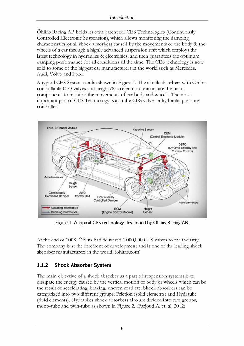
A typical CES System can be shown in Figure 1. The shock absorbers with Öhlins controllable CES valves and height & acceleration sensors are the main components to monitor the movements of car body and wheels. The most important part of CES Technology is also the CES valve - a hydraulic pressure controller.
Figure 1. A typical CES technology developed by Öhlins Racing AB.
At the end of 2008, Öhlins had delivered 1,000,000 CES valves to the industry. The company is at the forefront of development and is one of the leading shock absorber manufacturers in the world. (ohlins.com)
1.1.2 Shock Absorber System
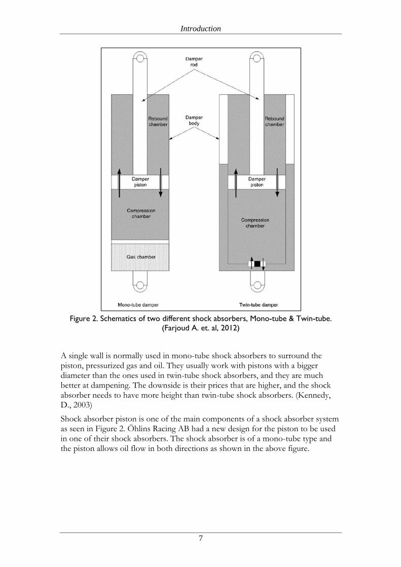
The main objective of a shock absorber as a part of suspension systems is to dissipate the energy caused by the vertical motion of body or wheels which can be the result of accelerating, braking, uneven road etc. Shock absorbers can be categorized into two different groups; Friction (solid elements) and Hydraulic (fluid elements). Hydraulics shock absorbers also are divided into two groups, mono-tube and twin-tube as shown in Figure 2. (Farjoud A. et. al, 2012)
Introduction
7
Figure 2. Schematics of two different shock absorbers, Mono-tube & Twin-tube.
(Farjoud A. et. al, 2012)
A single wall is normally used in mono-tube shock absorbers to surround the piston, pressurized gas and oil. They usually work with pistons with a bigger diameter than the ones used in twin-tube shock absorbers, and they are much better at dampening. The downside is their prices that are higher, and the shock absorber needs to have more height than twin-tube shock absorbers. (Kennedy, D., 2003)
Shock absorber piston is one of the main components of a shock absorber system as seen in Figure 2. Öhlins Racing AB had a new design for the piston to be used in one of their shock absorbers. The shock absorber is of a mono-tube type and the piston allows oil flow in both directions as shown in the above figure.
Introduction
8
1.1.3 Problems with the Current Part
The problem with the current design of the piston is that the intricate details on the piston are produced by machining. The estimated batch size of the product is 100,000/year. In fact, machining is not an economic and efficient way of manufacturing such a number of products. The company is looking for a cheaper and more efficient way of producing the shock absorber piston. Another problem is that, since machining produces very fine surfaces, the design had to include very thin wall thicknesses in order to avoid sliding. Rougher surfaces, faster & cheaper mass production, instead, were needed.
1.2 Purpose & Research Questions
The purpose of this thesis work is to investigate the possibility of adapting the existing design for Powder Metallurgy method in order to get a cheaper product while maintaining the same performance. In this regard, designing of the piston was to be done by the whole product development process starting by modeling in SolidWorks environment (3D-CAD modeling program), selecting the right material by searching the current database and similar products. The next step was to consult Callo Sintermetall AB to verify the feasibility of manufacturability of the design. Consequently, it will be followed by Finite Element Method analysis in ABAQUS. If the test results are satisfactory, the company can switch the manufacturing process from machining to P/M method and then reduce the cost significantly while decreasing the cycle time needed for manufacturing the parts.
How can this current machined shock absorber piston be redesigned and developed for Powder Metallurgy process so that it fulfills the technical requirements associated with it?
What approach would be more reliable to estimate the fatigue life for a P/M part?
1.3 Delimitations
The rest of the shock absorber components, properties of the oil, the friction between oil and the side walls and the friction between the piston and the tube walls are not covered. In fatigue analysis, frequency effects are not taken into consideration.
Theoretical background
9
2 Theoretical background
Upon consulting with Öhlins Racing AB, it was decided that we would propose two different designs aimed at two different price ranges.
The first one is a low-cost design which will use Conventional Press and Sintering as the manufacturing method, which is the most basic, cheapest and simplest method within P/M processes. In this case, the density range is from 82% to 95% of the wrought corresponding material. (Sonsino, 1994)
The second design will employ Metal Injection Moulding (MIM) as the manufacturing method. As we will discuss later, MIM allows very complex shapes, and it can reach densities up to 97% of the wrought counterpart, so improving the mechanical properties. (epma.com)
2.1 Basics of Powder Metallurgy
Powder Metallurgy (P/M) is a type of metalworking technology using metal powders as the main material. One of the biggest advantages of P/M process is its ability to manufacture net or near-net shape components with relatively high complexity by an economical method. Parts can be manufactured to close tolerances, with high utilization of material.
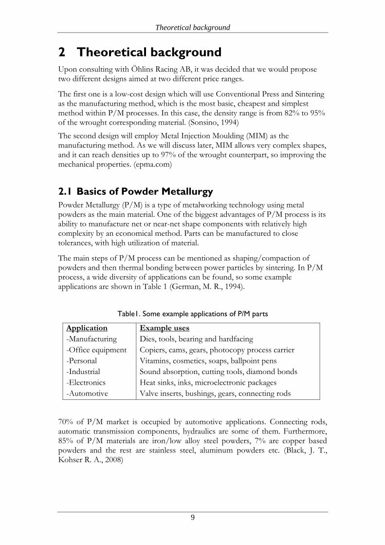
The main steps of P/M process can be mentioned as shaping/compaction of powders and then thermal bonding between power particles by sintering. In P/M process, a wide diversity of applications can be found, so some example applications are shown in Table 1 (German, M. R., 1994).
Table1. Some example applications of P/M parts
Application Example uses
-Manufacturing Dies, tools, bearing and hardfacing
-Office equipment Copiers, cams, gears, photocopy process carrier
-Personal Vitamins, cosmetics, soaps, ballpoint pens
-Industrial Sound absorption, cutting tools, diamond bonds
-Electronics Heat sinks, inks, microelectronic packages
-Automotive Valve inserts, bushings, gears, connecting rods
70% of P/M market is occupied by automotive applications. Connecting rods, automatic transmission components, hydraulics are some of them. Furthermore, 85% of P/M materials are iron/low alloy steel powders, 7% are copper based powders and the rest are stainless steel, aluminum powders etc. (Black, J. T., Kohser R. A., 2008)
Theoretical background
10
In fact, P/M is an advanced method for producing reliable ferrous and non-ferrous parts. The European market has an annual turnover more than Six Billion Euros while annual powder product is more than one million tones worldwide. The high precision forming ability of P/M process often makes it possible to eliminate the need for machining. A wide variety of P/M products can be manufactured by mixing diverse alloying and elemental powders, compacting in a die and finally sintering. (epma.com)
P/M methods also allow for unique mixtures of materials which are not possible with other manufacturing methods. This enables new opportunities for P/M process to be used in new and exciting products with specially tailored materials. (German, M. R., 1994)
Because of the homogenous structure it provides, P/M is also attractive to companies looking for more consistent, repeatable and predictable parts with high quality. The fact that the P/M process is growing can be attributed to cost savings which can be achieved through successful implementation of this process. In some cases, these cost savings can be up to 40% if a cast or wrought component is manufactured by P/M process.
P/M usually uses 97% of the starting raw material which adds to cost savings. Two main reasons for using P/M process are;
Cost savings compared to the other processes,
Unique properties which can only be achieved with P/M process.
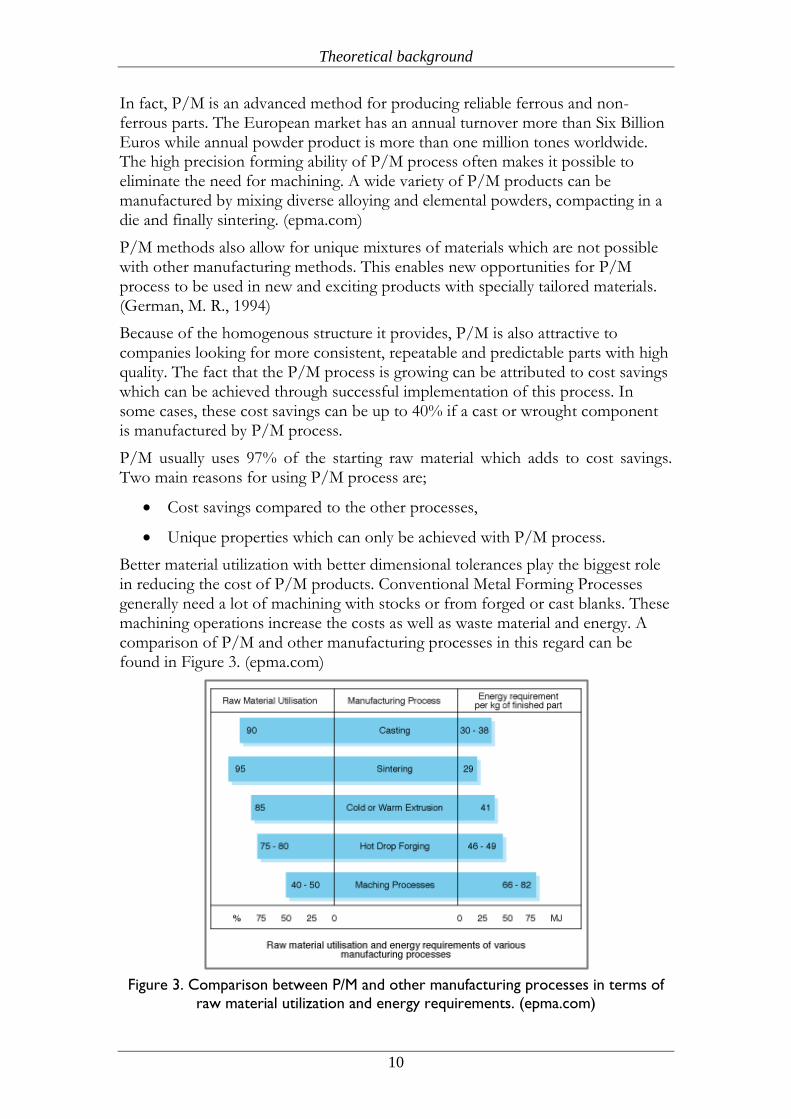
Better material utilization with better dimensional tolerances play the biggest role in reducing the cost of P/M products. Conventional Metal Forming Processes generally need a lot of machining with stocks or from forged or cast blanks. These machining operations increase the costs as well as waste material and energy. A comparison of P/M and other manufacturing processes in this regard can be found in Figure 3. (epma.com)
Figure 3. Comparison between P/M and other manufacturing processes in terms of
raw material utilization and energy requirements. (epma.com)
Theoretical background
11
Moreover, tooling wear is a major concern in P/M manufacturing methods, since metal powders tend to be abrasive. Thus, hardened tool steel is commonly used for P/M tooling components. Cemented carbide can be also used if the production rate is high and if the powders are too abrasive. Die surfaces should be highly polished. Dies and the tooling should be rigid enough to sustain the pressing pressures. (Black, J. T., Kohser R. A., 2008)
In P/M methods, powder densification of parts can be done in three different methods: sinter densifying a low density preform, pressing to a high density and then sintering, simultaneous sintering and pressing. Powders which show good sintering densification do not need very high pressures and can be pressed at low pressures. Metal Injection Molding (MIM) is such a process. The way of delivering this pressure to the powder, the rate of pressurization and the mechanical constraints play a big role in determining the final density of the pressed product. (German, M. R., 1994)
2.1.1 Strength Properties of P/M Parts
There are some aspects affecting the strength properties of P/M products. The most important of these are:
Density
Alloying elements
Sintering conditions
Heat treating conditions
Density is a very important factor in determining final properties of a P/M product. There is a linear relation between the density and tensile strength and fatigue strength. Elongation and impact strength increase exponentially with increased density.
Achievable density is dependent on the compacting pressure. Pressures higher than 650 MPa are not practical because of damaging the tool. Also, after a certain pressure, the increase in pressure will not be as effective as earlier.
In iron-based powder metallurgy, sintering is usually carried out in continuous belt furnaces at about 1120C degrees for usually 20-30 minutes. Sintering affects how efficient the powder particles weld to each other as well as the speed of the homogenization of alloying elements. In fact, alloying elements take part in forming microstructures and increasing the resistance to deformation. Different alloying elements, thus, can be used for achieving different results.
Although alloying elements have almost the same effect on sintered steels as conventional steels, not all elements can be used in sintering because some of them oxidize too easily in sintering atmospheres and have a negative impact on physical and mechanical properties.
Theoretical background
12
The choice of alloy composition should be made carefully according to required properties as well as dimensional stability. Resulting hardness is important in determining if the part can be sized or coined after sintering or not. Parts having the hardness with more than 150 HV are hard to size or coin.
Heat treating conditions should be selected and controlled carefully in order to have good dimensional stability. It’s important to have symmetric heating and cooling, otherwise the part will distort so severely that it might even be rejected. (Höganäs, 2007)
2.2 Conventional Press and Sintering
Conventional Press and Sintering is one of the P/M methods in order to produce P/M parts with the simplest geometrical complexity and the lowest cost.
In general, Conventional Powder Metallurgy processes can be divided into four main stages discussed later in this chapter;
Powder Manufacturing
Mixing/Blending
Compaction
Sintering
Post-sintering operations (machining, drilling, sizing, coining, etc.) can be also considered as important steps in P/M methods. (Black, J. T., Kohser R. A., 2008)
2.2.1 Manufacturing Steps of Conventional Press and Sintering
There are five main steps to describe Conventional Press and Sintering manufacturing process as the followings:
Powder Manufacturing
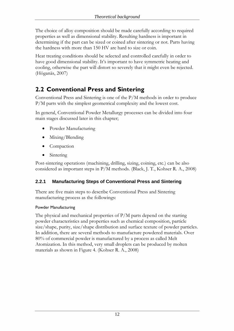
The physical and mechanical properties of P/M parts depend on the starting powder characteristics and properties such as chemical composition, particle size/shape, purity, size/shape distribution and surface texture of powder particles. In addition, there are several methods to manufacture powdered materials. Over 80% of commercial powder is manufactured by a process as called Melt Atomization. In this method, very small droplets can be produced by molten materials as shown in Figure 4. (Kohser R. A., 2008)
Theoretical background
13
Figure 4. Melt Atomization Method to produce metal powders.
There are some factors which help us assess the quality of the powder. Flow rate, apparent density, compressibility, green strength and so on. Firstly, flow rate is the ability of the powder to fill the die. If it is poor, the die filling will be non-uniform, resulting in a non-uniform density. Secondly, apparent density is the density of the powder prior to pressing. Thirdly, compressibility is the effect by which the powder can be pressed and densified, and finally green strength is the strength of the component after compacting, before sintering. Good green strength is needed to maintain sharp corners, smooth surfaces and intricate details. (Black, J. T., Kohser R. A., 2008)
Mixing
After the manufacture of powder, it is time for mixing. Mixing is where the lubricant is added, and a homogenous structure is achieved. Stearic acid, stearin, metallic stearates and other organic compounds can be used as lubricants.
Main objective of adding the lubricant is to reduce the friction between the powder mass and the tools; therefore, assisting in achieving a uniform density can be made. Lubricants also aid in ejecting the part and minimize the tendency to form cracks.
Over-mixing (adding more than enough lubricant) should be avoided because it will increase the apparent density. It is also detrimental to green strength because if the lubricant covers the whole surface of particles it will prevent metal from contacting to metal. (epma.com)
Theoretical background
14
Compacting
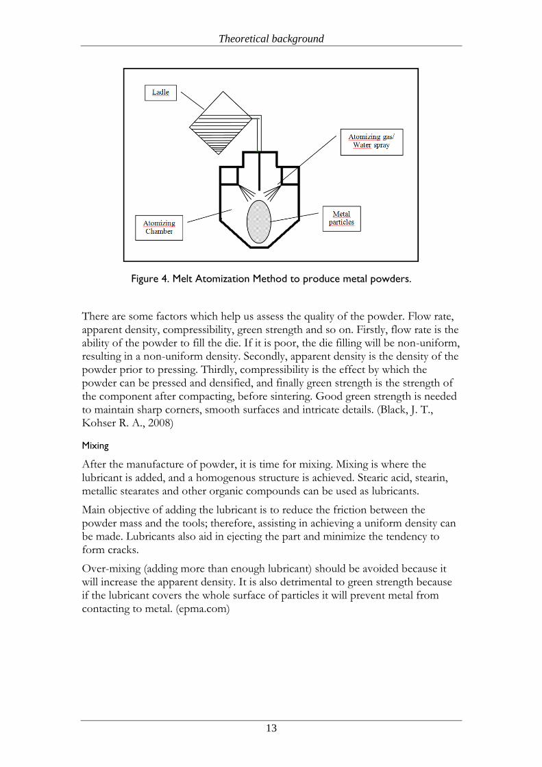
Before discussing about compaction, the different classes of the complexity of P/M products can be categorized. Class 1 being the one-level simplest parts and they are compressed easily from one direction. The thickness of such parts is supposed to be kept under 6.35 mm. Class 2 parts can be considered as thicker one-level with any thickness, so they are normally compressed in dies from two directions , while Class 3 being the two-level parts requiring two-direction compaction. Finally Class 4 is the most complex multi-level part, and they are necessarily compressed at multi-pressing motions as shown in Figure 5. The shock absorber piston in this project has different levels, different thicknesses, through holes and blind holes, therefore it is a class 4 component and needs relatively complicated tooling and punches. (Black, J. T., Kohser R. A., 2008)
Figure 5. Sample P/M parts with different geometrical classes. (Black, J. T., Kohser R.
A., 2008)
To compact the powder mass in a die (e.g. made of rigid steel or carbide), the pressures between 150 and 900 MPa are normally used. In this stage, the green compact are produced by the mechanical interlocking and cold-welding between powder particles. After compaction, parts should have sufficient strength for further handling. (epma.com)
Class 1
Class 2
Class 3
Class 4
Theoretical background
15
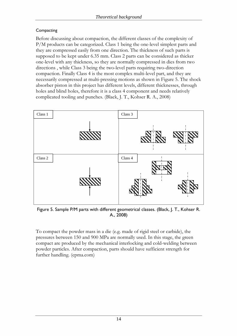
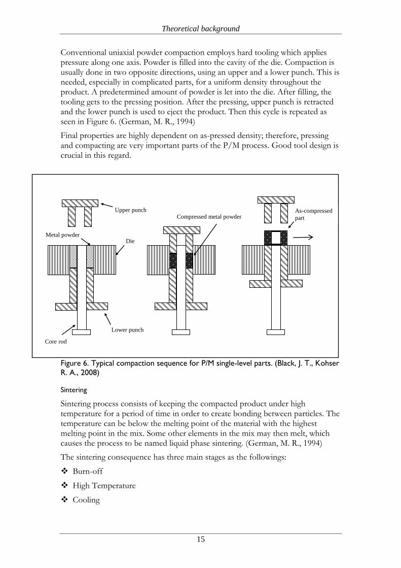
Conventional uniaxial powder compaction employs hard tooling which applies pressure along one axis. Powder is filled into the cavity of the die. Compaction is usually done in two opposite directions, using an upper and a lower punch. This is needed, especially in complicated parts, for a uniform density throughout the product. A predetermined amount of powder is let into the die. After filling, the tooling gets to the pressing position. After the pressing, upper punch is retracted and the lower punch is used to eject the product. Then this cycle is repeated as seen in Figure 6. (German, M. R., 1994)
Final properties are highly dependent on as-pressed density; therefore, pressing and compacting are very important parts of the P/M process. Good tool design is crucial in this regard.
Figure 6. Typical compaction sequence for P/M single-level parts. (Black, J. T., Kohser
R. A., 2008)
Sintering
Sintering process consists of keeping the compacted product under high temperature for a period of time in order to create bonding between particles. The temperature can be below the melting point of the material with the highest melting point in the mix. Some other elements in the mix may then melt, which causes the process to be named liquid phase sintering. (German, M. R., 1994)
The sintering consequence has three main stages as the followings:
Burn-off
High Temperature
Cooling
Die
Upper punch
Lower punch
Core rod
Metal powder
Compressed metal powder As-compressed
part
Theoretical background
16
During the first stage (burn-off) lubricants and binders are burnt off and removed from as-compressed parts, and then in High temperature stage the welding of the particles to each other takes place.
Cooling period is, then, used to prevent the thermal shock which the component would have if it went directly from high temperature to room temperature. (Black, J. T., Kohser R. A., 2008)
Sintering is usually done in a continuous belt furnace. However, there have been some developments in this area, and microwaves can be used for sintering as well. The process where the microwave technology is used to sinter products is called Microwave Sintering.
Microwave sintering is a rather new variation of sintering method. Although the microwave sintering of ceramics started as early as 1967, application of this method to metallic powder materials happened only in recent years.
Microwave sintering has some obvious advantages over conventional sintering. Rapid & effective heating, time & energy saving and the ability to reach high temperatures with a relatively low temperature in the applicator are some of these advantages.
A. Nadjafi Maryam Negari et. al. compared a mixture of Fe-Cu powder sintered with microwave sintering and conventional sintering. They found out that the density of the microwave sintered powders were higher than the conventionally sintered ones. The yield strength, hardness and microhardness of the microwave sintered samples were also about 10% higher than the conventionally sintered ones. It was also shown that microwave sintering was faster than the conventional sintering. Microstructure of the microwave sintered powders was much finer and more uniform than the conventionally sintered counterparts. Pore distribution was also better in microwave sintered samples, having rounded pores, while in conventional sintering the powders had sharp edges pores with non-uniform distribution. (Negari, M. N. A., et. al., 2007)
For microwave sintering purposes, frequency bands around 915 MHz, 2.45 GHz, 28 GHz and 80 GHz are permitted. Another advantage of microwave processing is the opportunity to heat the component uniformly. Peng Yuandong et. al. experimented on Fe-2Cu-0.6C powder sintered by microwave radiation and conventional sintering. Microwave sintering was carried out for 10 minutes at 1150C degrees while conventional sintering was done in a molybdenum-sintering furnace at the same temperature for 60 minutes.
In conventionally sintered sample, the resulting density was 6.94 gr/cm3, while in microwave sintered one it was 7.2 gr/cm3. Depending on density and finer microstructure, tensile strength, hardness and elongation of the sintered powder were all significantly better than the conventionally sintered sample. Moreover, it was carried out only in 10 minutes. The tensile strength of the conventionally sintered sample was 266 MPa, while the microwave sintered sample had 413 MPa. Elongation also increased from 2.2% to 6.0%. (Yuandong, P., et. al., 2009)
Theoretical background
17
There are numerous factors which may interfere with the electromagnetic field and the way the components are heated, resulting in a difficulty of repeatability of the same quality in all components. (Leonelli, C., et. al., 2008)
It has been suggested that in order for microwave sintering process to be attractive, the product should be large or have wide thickness, the material should be expensive, electricity should be cheap and the improvements by using microwave sintering should be significant.
The use of microwave sintering is hindered by high process cost and inefficient electric power. Successful use of microwave sintering arises after improvement of material’s properties, savings in time, space and capital equipment. The decision to use microwave sintering has to be made after analyzing the process for each product individually. (National Research Council (U.S.), 1994)
Post-Sintering Operations
The physical and mechanical properties of P/M products can be improved by a wide range of post-sintering operations after sintering. Mechanical Surface Densification and Heat Treatment can be mentioned as two main post-sintering operations for strength improvement of P/M parts. To reach a better improved strength, the surface layers can be densified by some operations like sizing, coining, surface rolling, shot peening etc. On the other hand, post-sintering heat treatments can increase both the static and fatigue strength with other operations such as quenching and tempering, Carbo-Nitriding, Carburizing, Nitriding, plasma-Nitriding, induction hardening etc.(Sonsino, C. M., 1994)
Sizing is one of post-sintering operations employed in order to reach better dimensional tolerances. In this case, parts are pressed once more after sintering. During re-pressing, density will increase as well. This is important in some structural parts where better properties in connection with higher densities are needed.
Hot re-pressing is a variation of re-pressing which can give better densification but worse dimensional tolerances. (epma.com)
2.2.2 Design for Conventional Press and Sintering
There are some design guidelines that should be considered while designing the parts to be produced by P/M process. We have focused on some of them really involved in this project, and some others will be briefly mentioned.
Although there are some design restrictions which one should take into account while designing P/M parts, it is possible to adapt existing designs into suitable designs for P/M. For this, there are some criteria which we should keep in mind as the followings:
The batch size should be big enough to make up for the tooling costs,
Shape and the dimensional tolerances of the part should be examined, and necessary changes should be made,
Physical & mechanical property requirements should be attainable with P/M,
Theoretical background
18
Calculate to see if indeed P/M is cheaper than other methods.
It is almost impossible to improve on all of these issues. Usually we have to sacrifice one aspect, in order to improve the other. (Höganäs, 2007)
Length-to-Width ratio is one important aspect in design for Conventional Press & Sintering. Applied pressure, and corresponding densification created by this pressure, decreases over the length of the product. Upper and lower punches are utilized in order to minimize this problem. However, the length-to-width ratio should not exceed 3:1 if possible.
Re-entrant grooves and reverse tapers cannot be manufactured directly with P/M process because it would be impossible to eject products from dies. Therefore, such features should be machined after sintering.
Abrupt changes in sections should be avoided as they tend to increase stresses and may lead to cracks upon ejection from dies. Sections should be as uniform as possible.
Capacity of presses available directly influences size of the parts which can be pressed. There is also a direct relation between production rates and simplicity of products. The simpler products are, the easier it is to press at high speeds. (epma.com)
2.2.3 Holes
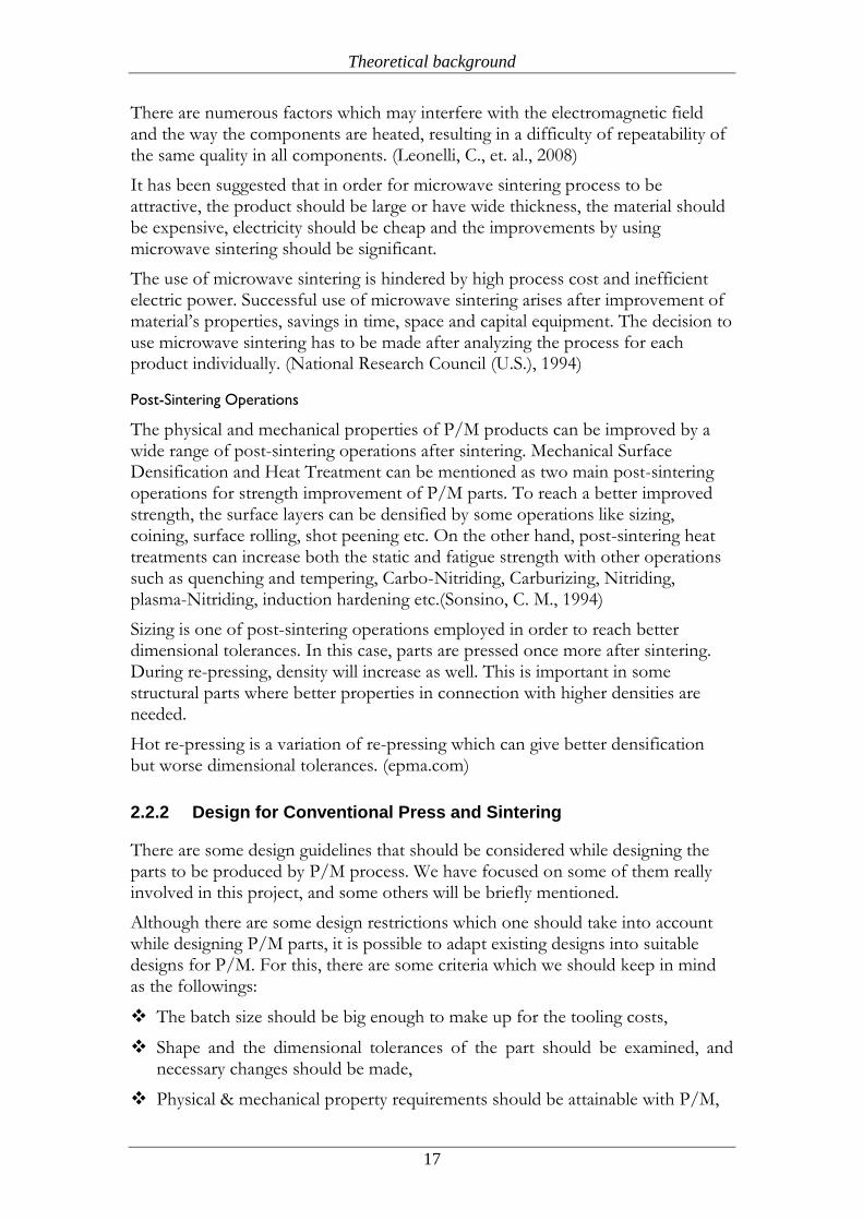
Holes are produced with the help of core rods in P/M. Although any kind of shapes can be made with core rods, round holes are preferable in that the tooling is much easier to produce as shown in Figure 7. (Höganäs, 2007)
In our current task as low-cost design, we have tried incorporating round holes into the part, but because of other requirements from the piston (e.g. maximizing the oil flow rate between compression and rebound chambers, meaning the holes should be as big as possible) we have decided to have polygonal holes.
Figure 7. Simple rounded holes are easily produced. (Höganäs, 2007)
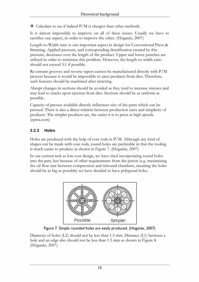
Diameter of holes (L2) should not be less than 1.5 mm. Distance (L1) between a hole and an edge also should not be less than 1.5 mm as shown in Figure 8. (Höganäs, 2007)
Theoretical background
19
Figure 8. Minimum diameter of holes and distance between holes from an edge.
(Höganäs, 2007)
In current Öhlins design (the machined piston), there are many holes with the radius from 1.4 to 1.8 mm, so we have eliminated all the holes for the new design to improve the robustness of piston & tooling design, and as mentioned earlier to increase the oil flow rate in the shock absorber while working.
2.2.4 Spring back effect
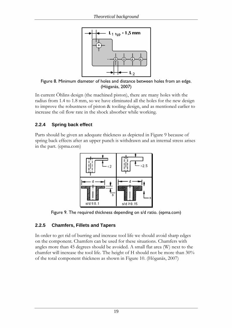
Parts should be given an adequate thickness as depicted in Figure 9 because of spring back effects after an upper punch is withdrawn and an internal stress arises in the part. (epma.com)
Figure 9. The required thickness depending on s/d ratio. (epma.com)
2.2.5 Chamfers, Fillets and Tapers
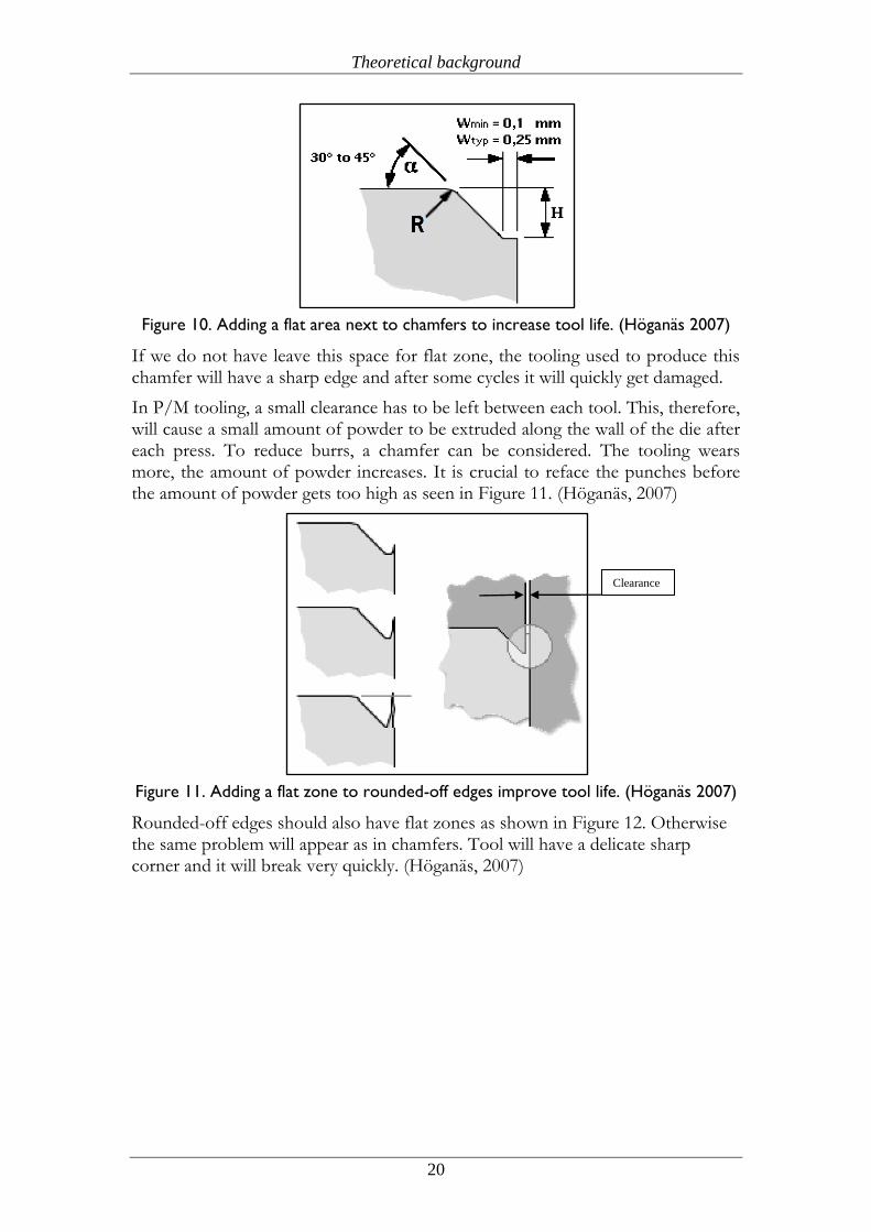
In order to get rid of burring and increase tool life we should avoid sharp edges on the component. Chamfers can be used for these situations. Chamfers with angles more than 45 degrees should be avoided. A small flat area (W) next to the chamfer will increase the tool life. The height of H should not be more than 30% of the total component thickness as shown in Figure 10. (Höganäs, 2007)
Theoretical background
20
Figure 10. Adding a flat area next to chamfers to increase tool life. (Höganäs 2007)
If we do not have leave this space for flat zone, the tooling used to produce this chamfer will have a sharp edge and after some cycles it will quickly get damaged.
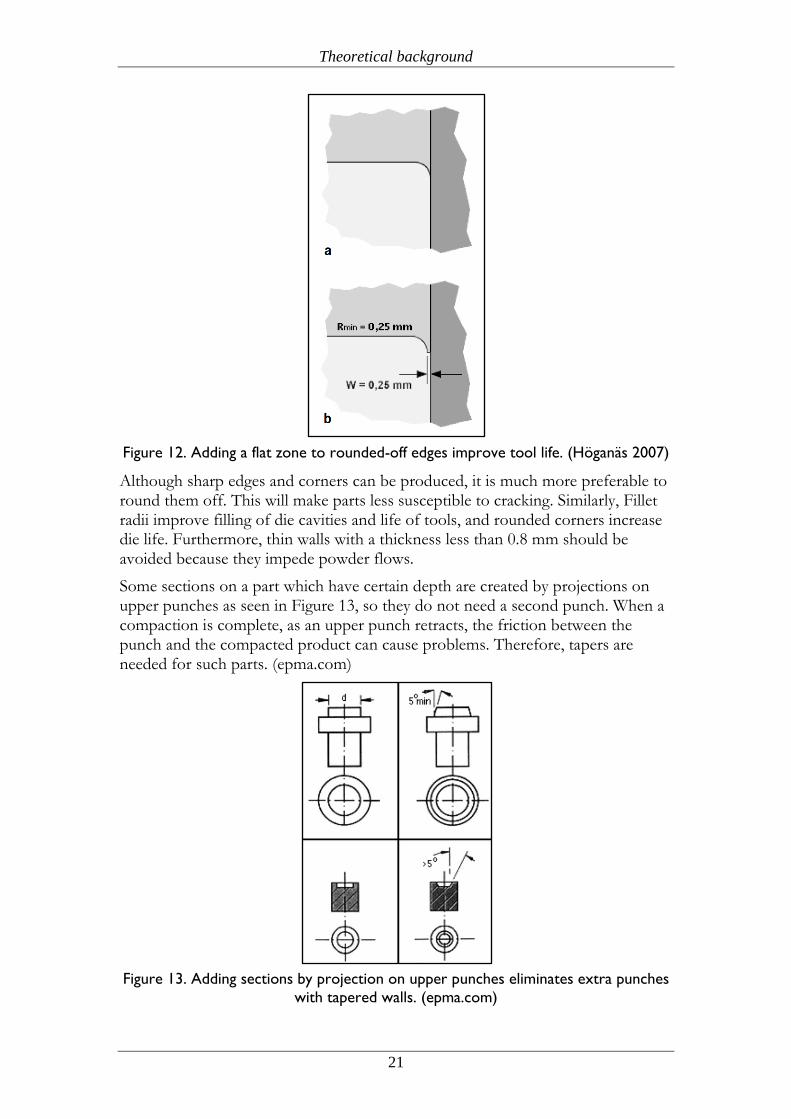
In P/M tooling, a small clearance has to be left between each tool. This, therefore, will cause a small amount of powder to be extruded along the wall of the die after each press. To reduce burrs, a chamfer can be considered. The tooling wears more, the amount of powder increases. It is crucial to reface the punches before the amount of powder gets too high as seen in Figure 11. (Höganäs, 2007)
Figure 11. Adding a flat zone to rounded-off edges improve tool life. (Höganäs 2007)
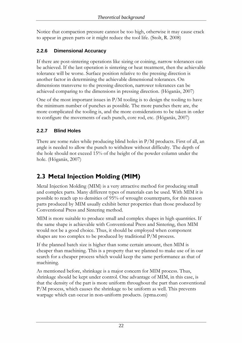
Rounded-off edges should also have flat zones as shown in Figure 12. Otherwise the same problem will appear as in chamfers. Tool will have a delicate sharp corner and it will break very quickly. (Höganäs, 2007)
Clearance
Theoretical background
21
Figure 12. Adding a flat zone to rounded-off edges improve tool life. (Höganäs 2007)
Although sharp edges and corners can be produced, it is much more preferable to round them off. This will make parts less susceptible to cracking. Similarly, Fillet radii improve filling of die cavities and life of tools, and rounded corners increase die life. Furthermore, thin walls with a thickness less than 0.8 mm should be avoided because they impede powder flows.
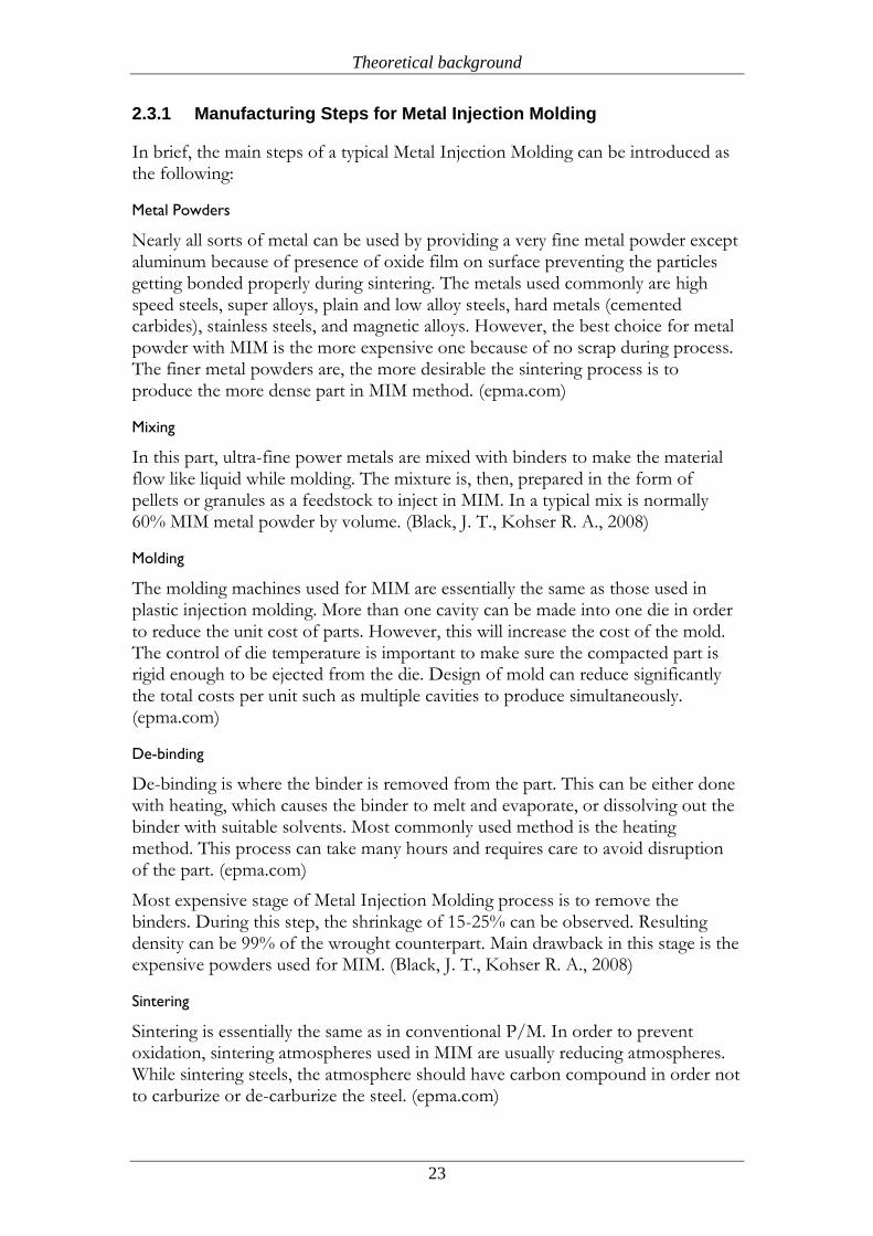
Some sections on a part which have certain depth are created by projections on upper punches as seen in Figure 13, so they do not need a second punch. When a compaction is complete, as an upper punch retracts, the friction between the punch and the compacted product can cause problems. Therefore, tapers are needed for such parts. (epma.com)
Figure 13. Adding sections by projection on upper punches eliminates extra punches
with tapered walls. (epma.com)
Theoretical background
22
Notice that compaction pressure cannot be too high, otherwise it may cause crack to appear in green parts or it might reduce the tool life. (Stolt, R. 2008)
2.2.6 Dimensional Accuracy
If there are post-sintering operations like sizing or coining, narrow tolerances can be achieved. If the last operation is sintering or heat treatment, then the achievable tolerance will be worse. Surface position relative to the pressing direction is another factor in determining the achievable dimensional tolerances. On dimensions transverse to the pressing direction, narrower tolerances can be achieved comparing to the dimensions in pressing direction. (Höganäs, 2007)
One of the most important issues in P/M tooling is to design the tooling to have the minimum number of punches as possible. The more punches there are, the more complicated the tooling is, and the more considerations to be taken in order to configure the movements of each punch, core rod, etc. (Höganäs, 2007)
2.2.7 Blind Holes
There are some rules while producing blind holes in P/M products. First of all, an angle is needed to allow the punch to withdraw without difficulty. The depth of the hole should not exceed 15% of the height of the powder column under the hole. (Höganäs, 2007)
2.3 Metal Injection Molding (MIM)
Metal Injection Molding (MIM) is a very attractive method for producing small and complex parts. Many different types of materials can be used. With MIM it is possible to reach up to densities of 95% of wrought counterparts, for this reason parts produced by MIM usually exhibit better properties than those produced by Conventional Press and Sintering method.
MIM is more suitable to produce small and complex shapes in high quantities. If the same shape is achievable with Conventional Press and Sintering, then MIM would not be a good choice. Thus, it should be employed when component shapes are too complex to be produced by traditional P/M process.
If the planned batch size is higher than some certain amount, then MIM is cheaper than machining. This is a property that we planned to make use of in our search for a cheaper process which would keep the same performance as that of machining.
As mentioned before, shrinkage is a major concern for MIM process. Thus, shrinkage should be kept under control. One advantage of MIM, in this case, is that the density of the part is more uniform throughout the part than conventional P/M process, which causes the shrinkage to be uniform as well. This prevents warpage which can occur in non-uniform products. (epma.com)
Theoretical background
23
2.3.1 Manufacturing Steps for Metal Injection Molding
In brief, the main steps of a typical Metal Injection Molding can be introduced as the following:
Metal Powders
Nearly all sorts of metal can be used by providing a very fine metal powder except aluminum because of presence of oxide film on surface preventing the particles getting bonded properly during sintering. The metals used commonly are high speed steels, super alloys, plain and low alloy steels, hard metals (cemented carbides), stainless steels, and magnetic alloys. However, the best choice for metal powder with MIM is the more expensive one because of no scrap during process. The finer metal powders are, the more desirable the sintering process is to produce the more dense part in MIM method. (epma.com)
Mixing
In this part, ultra-fine power metals are mixed with binders to make the material flow like liquid while molding. The mixture is, then, prepared in the form of pellets or granules as a feedstock to inject in MIM. In a typical mix is normally 60% MIM metal powder by volume. (Black, J. T., Kohser R. A., 2008)
Molding
The molding machines used for MIM are essentially the same as those used in plastic injection molding. More than one cavity can be made into one die in order to reduce the unit cost of parts. However, this will increase the cost of the mold. The control of die temperature is important to make sure the compacted part is rigid enough to be ejected from the die. Design of mold can reduce significantly the total costs per unit such as multiple cavities to produce simultaneously. (epma.com)
De-binding
De-binding is where the binder is removed from the part. This can be either done with heating, which causes the binder to melt and evaporate, or dissolving out the binder with suitable solvents. Most commonly used method is the heating method. This process can take many hours and requires care to avoid disruption of the part. (epma.com)
Most expensive stage of Metal Injection Molding process is to remove the binders. During this step, the shrinkage of 15-25% can be observed. Resulting density can be 99% of the wrought counterpart. Main drawback in this stage is the expensive powders used for MIM. (Black, J. T., Kohser R. A., 2008)
Sintering
Sintering is essentially the same as in conventional P/M. In order to prevent oxidation, sintering atmospheres used in MIM are usually reducing atmospheres. While sintering steels, the atmosphere should have carbon compound in order not to carburize or de-carburize the steel. (epma.com)
Theoretical background
24
2.3.2 Design for Metal Injection Molding (MIM)
Designing for Metal Injection Molding (MIM) has some different requirements comparing to Conventional Press and Sintering. Uniform wall thicknesses are desired in order to avoid cracking, distortion and internal stresses. Similarly, shrinkage can be a main issue in MIM methods, and the part can shrink up to 20% after sintering. Thus, if the wall thicknesses are not uniform, shrinkage will not be uniform either, so this should be avoided as much as possible. Otherwise, the transition from thicker to thinner walls should be made gradually. Sudden changes also should be avoided.
Other issues such as sharp corners should be avoided because they can act as stress raisers. Fillets and radii can be utilized in order to avoid this while assisting in the ejection of the part from the mold, improving the strength of parts and the aesthetics as well. Radii less than 0.127 mm will be hard to produce in molds and will cause stress concentrations. Thus, radii should be kept bigger than 0.127 mm.
From the economical point of view, size of the MIM parts should be as small as possible in order to reduce the cost because the very fine powders which form the base materials for MIM are expensive. (epma.com)
Metal Injection Molding method combines the shaping capability of Plastic Injection Molding process with the mechanical properties of wrought metal materials. It’s being used in a wide variety of applications including automotive fuel & ignition systems, aerospace & defense systems, dental instruments, power hand-tools, pumps and so forth.
While designing for MIM, we should ignore the limitations for traditional metalworking processes. We have the freedom to put material only where it is needed for functionality and strength. In fact, since the very fine powders used for MIM are expensive, any opportunity to minimize the amount of material in the product should be taken.
Sintering supports are needed for some parts because of excessive shrinkage which may cause the parts to distort. This may happen to the parts which do not have a wide flat surface. In this case, such parts need sintering supports which increase the overall cost of the product. Since our shock absorber piston has a flat surface which it can rest upon, it does not need any sintering support.
MIM parts do not require draft. This is because the metal powders keep the heat long after it has been ejected from the mold, so the post molding shrinkage happens several minutes after the part has been ejected. This prevents the part from shrinking around cores and other mold features. Lubricants inside the mix also help in ejection which further reduces the need for drafts. However, drafts may still need to be used in some situations, such as holes deeper than 0.25 inch.
Holes and slots can be easily incorporated into MIM products without adding to the piece price. However, molds will be more complicated and thus more expensive to produce. Holes that are perpendicular to the parting line are the easiest to produce and they should be preferred.
Theoretical background
25
A minimum wall thickness of 0.25 mm is possible, but it depends on the overall size of the part. Generally, the wall thicknesses vary between 1 and 3 mm. In addition, minimizing the wall thickness is important in that the material amount and therefore the cost of the product can be reduced. (Kinetics, 2004)
2.4 Properties of Sintered iron-based materials
Ni, Cu, Mo, P and C are the most commonly used alloying elements in P/M steels. It’s important to note that Cu and P are harmful for ingot steels, but they can be used without problems in powder form and they have good strengthening effects. Elements like Mn, Cr and V should be added with care in order to avoid oxidation.
P/M materials contain pores which reduce the overall properties of the material. This strength loss can be made up for with the addition of alloying elements. These alloying elements can be concentrated around the pores, locally improving the strength.
Densities of P/M steels for structural parts are usually between 6.4 - 7.7 gr/cm3. In lower densities, the pores may be interconnected. Thus, this may lead to gaseous or liquid materials to infiltrate into the open pores. In order to avoid this possibility, these pores may need to be filled. Infiltration is one method which can be used in this case. This is done through infiltrating the part with a metal which has lower melting temperature than the sintering temperature.
Most mechanical properties decrease with increasing porosity, but the size, shape and distribution of these pores are also important. For example, large rounded pores with a uniform distribution are less harmful than smaller pores with sharp edges and non-uniform distribution.
Another issue is the hardness of P/M structural parts directly related to density, microstructure and chemical composition.
Young’s modulus is also approximately a linear function of the density. Like in solid steels, Young’s modulus does not change significantly with alloying elements.
The fatigue strength of P/M steels increases with increasing density. The composition does not affect it significantly. In fact, between the most commonly used medium strength P/M steels there is approximately 20% difference. The decrease of fatigue strength with increased notch factor in P/M steels is not as big as wrought steels. Since the material is porous, it’s not as sensitive to external notches as fully solid materials.
Loading mode is another factor in determining fatigue strength. Under bending loading, fatigue strength is higher than in axial loading. This is because the most stressed material’s volume is small, decreasing the number of defects which can act as failure starters. Therefore it was important for us to determine the mode of loading first. (Sonsino, C. M., Esper, F. J., 1994)
Theoretical background
26
The current shock absorber piston in this project is fixed in the middle in connected with the shock absorber rod, while having its sides free. Pressure is applied on sides, thereby creating a bending loading mode, and then it results the more fatigue strength. It will be discussed extensively later in the chapter 4.2.
2.5 Improving the Strength of P/M Steels
Shot peening, sizing, coining operations can densify the surface layers of the part, and thus improve fatigue strength. The more severe the densification is, the more improvement we get. Phenomena which have a significant effect in increasing the fatigue strength are surface densification, increasing hardness and accumulation of residual stresses. Similarly, it has been shown that the endurance limit can be raised by 22% with shot peening.
It is also possible to apply sizing only to certain areas of the component to increase the fatigue strength of that specific area. This can be useful when critical areas in the part are known.
Surface rolling has been shown to increase the fatigue strength of the component by a factor of 2.2. The strengthening effect of surface rolling seems considerably larger than that of sizing or shot peening, because bigger residual stresses are induced by this method.
The effect of surface rolling is also stronger in low-density components, making this method a very effective way of improving the low strength P/M steels so that they can meet the requirements for higher strength applications. This makes surface rolling an attractive alternative for our part as well. If we cannot obtain a density more than 6.8 gr/cm3, we will either use an expensive powder with a different alloyed composition or need to improve the properties of our powder with post-sintering operations. Since surface rolling has greater effect on low-density P/M steels, it might be a good choice for the low-cost piston.
Heat treatment is another way of improving the properties of the sintered material. There are different ways of heat treating the sintered component, including quenching and tempering, Carbo-Nitriding, Carburizing, induction hardening etc. Some experiments show that Carbo-Nitriding is the most effective in increasing the fatigue strength. (Sonsino, C. M., Esper, F. J., 1994)
Another cost-effective way of increasing the density and, therefore, improving the properties of P/M steels is warm compaction. The die and the powder are heated
to about 130-150 degrees.
Lubricants are used in press and sintering in order to aid in ejection of the part as well as helping the compaction of powders. However, they should not be used excessively as they tend to reduce the mechanical properties. They also have to be burnt off at the beginning of the sintering stage.
Instead of mixing the lubricants directly in the powder, some researchers suggested that only the die wall may be lubricated. This would avoid the possible entrapment of lubricants in the powder which reduces the mechanical properties.
Theoretical background
27
It has been shown that using die wall lubrication instead of admixed powder, coupled with warm compaction increases density, thereby increasing the mechanical properties of P/M steels. (Babakhani, A., Haerian, A., Ghambari, M., 2006)
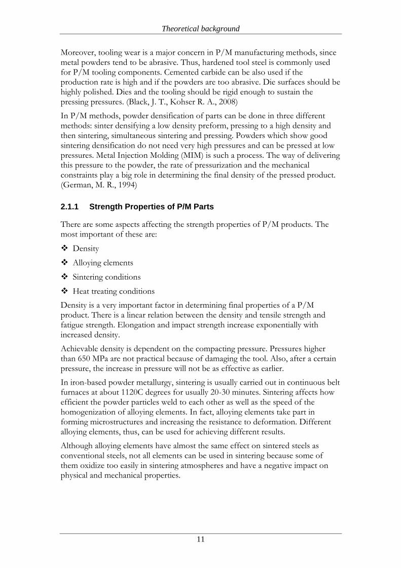
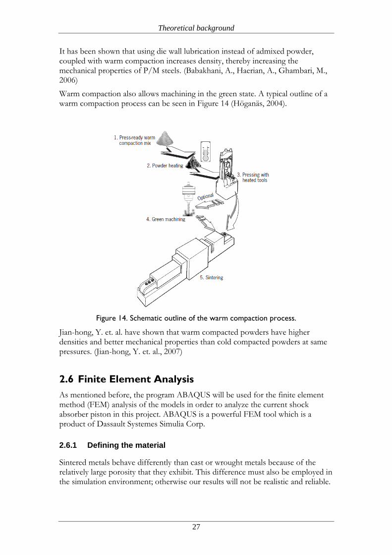
Warm compaction also allows machining in the green state. A typical outline of a warm compaction process can be seen in Figure 14 (Höganäs, 2004).
Figure 14. Schematic outline of the warm compaction process.
Jian-hong, Y. et. al. have shown that warm compacted powders have higher densities and better mechanical properties than cold compacted powders at same pressures. (Jian-hong, Y. et. al., 2007)
2.6 Finite Element Analysis
As mentioned before, the program ABAQUS will be used for the finite element method (FEM) analysis of the models in order to analyze the current shock absorber piston in this project. ABAQUS is a powerful FEM tool which is a product of Dassault Systemes Simulia Corp.
2.6.1 Defining the material
Sintered metals behave differently than cast or wrought metals because of the relatively large porosity that they exhibit. This difference must also be employed in the simulation environment; otherwise our results will not be realistic and reliable.
Theoretical background
28
There are different material models available for use in ABAQUS software. The ones that we can use for sintered metals are Porous Metal Plasticity model and Porous Elastic material model. Since we are not going to use any plastic material properties in our simulations, we will use Porous Elastic Material model. In order to assess the fatigue life of our component, we will run static simulations in the elastic region, determine which region of the component is subjected to the highest local stress amplitude & the corresponding mean stress and use this data to establish the Haigh diagram where we can see if our product is in the safe or unsafe region as all will be discussed later in this chapter.
For simulating MIM products, we can use Linear Elastic Material model since the relative density of MIM products can be up to 95%. Therefore, the effect of pores is not so significant.
Porous Elastic Material Model
In ABAQUS, there are two ways to define the deviatoric (related to shape changes) elastic behavior of a porous material. One of these is to define it by using Shear Modulus and the other is by using Poisson’s Ratio. Since the data for Poisson’s Ratio for powder metals is readily available, we will define our material in this way.
In this model, we have to define the following material parameters in ABAQUS;
Logarithmic bulk modulus
Poisson’s Ratio
Tensile limit.
Additionally we have to define the Initial Void Ratio of the porous material, which is the ratio of pores in the material. However, this cannot be done in ABAQUS CAE environment, and we have to make changes in the input file. For each job that we are running, we will first write an input file for that job and then edit that input file to include the Initial Void Ratio and the element set for which this void ratio is valid, which includes the whole elements in the product.
Linear Elastic Material Model
Linear elastic material model is the most straightforward material model in ABAQUS which is used to define the behavior of isotropic materials. (ABAQUS Analysis User’s Manual)
The only parameters we need in order to define the material model are;
Young’s Modulus
Poisson’s Ratio.
2.6.2 Assessment of different Loading modes
In order to assess the durability of the piston correctly, we have to carry out both a static and a dynamic analysis.
Theoretical background
29
Static Loading Mode
For the static loading, we will apply a static uniform pressure on both sides of the low-cost and the high-performance piston respectively on the certain areas in ABAQUS. This kind of pressure can be considered as a hyrostatic pressure because of pressurized oil on both sides of the piston. In this case, we must determine the maximum local stress concentration area of the piston and then compare it with the allowable values for the yield strength.
Dynamic Loading Mode
For dynamic analysis, there are two cyclic loads with different frequencies being considered to design the pistons. These two different cases, which were provided by Öhlins Racing AB, simplify the actual varying loads that act on the piston. We should take into account that the alternating forces acting on the different sides are not equal to each other. The fatigue failure analysis will be the next step.
Stress-Based Fatigue Analysis
Parts subjected to dynamic loading may break even at very low load levels. These kinds of load levels can be far below UTS (Ultimate Tensile Strength) or YS (Yield Strength) of the materials. This kind of failure is normally called Fatigue. This phenomenon has been dealt with by engineers for more than 150 years, and it should be mentioned that fatigue failure is still very common in industry now a days. Furthermore, nearly 60 to 90 percent of all mechanical failures of components can be considered due to fatigue. (Dahlberg, T., 2002)
In cyclic loading, the type of load variation normally is sinusoidal. In addition, there are only two important values in the form of load variation. Mean stress ( )
and Stress amplitude ( ) in materials are both of them as shown in Formula 1.
The stress in the material under cyclic loading varies between the two limits, the
maximum stress ( ) and the minimum stress ( ).
) and
) Formula (1)
Furthermore, Stress ratio (R) and Stress range ( ) as seen in Formula 2.
R=
and =2 Formula (2)
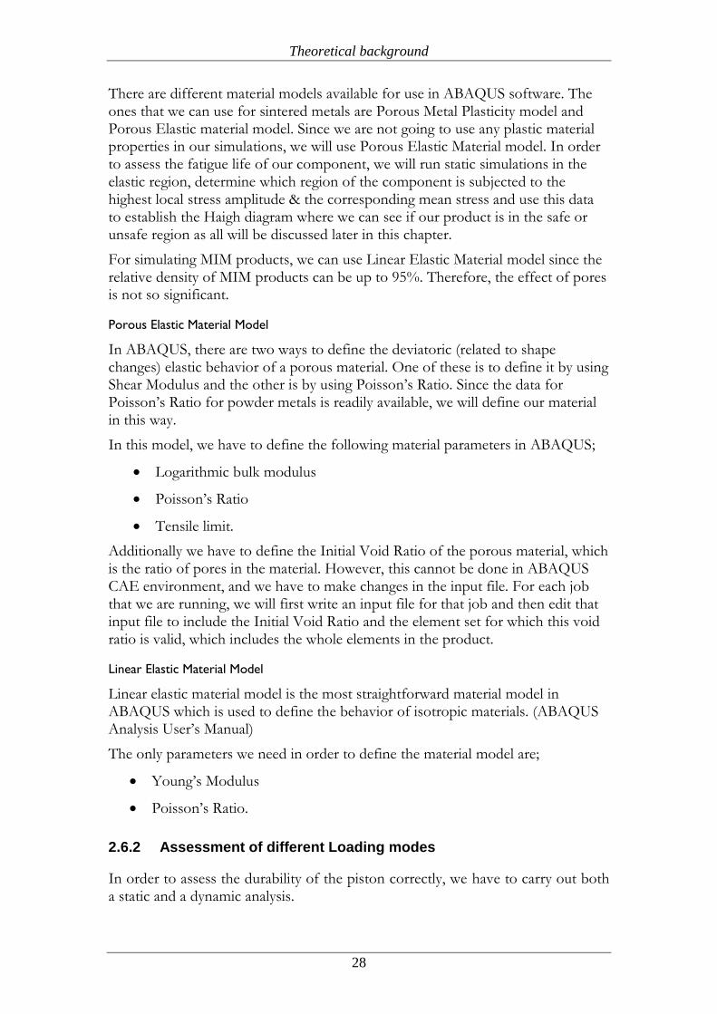
The fatigue data of the material are given for mostly two different loading types: alternating and pulsating. In alternating, fully reversed loading, the mean stress has a zero value ( =0, ≠0) as shown in Figure 15 (a). On the other hand, pulsating loading provides a zero value for the minimum stress ( =0, ≠0), and the mean
stress is equal to the stress amplitude ( = ) as seen in Figure 15 (b). In addition, there is a general definition for a typical cyclic loading in which the mean stress and stress amplitude are not zero as shown in Figure 15 (c). (Dahlberg, T., 2002)
Theoretical background
30
Figure 15. (a) Alternating (fully reversed) stress when R=-1, (b) Pulsating stress when
R=0 and (c) periodically fluctuating stress when R 0.
In this project, the cyclic loads on the piston for both frequencies are defined as general periodically fluctuating stresses by Öhlins Racing AB, where the stress ratios and the mean stresses will not be zero, and more details will be discussed later in the next chapters.
Wöhler diagram (S-N curve)
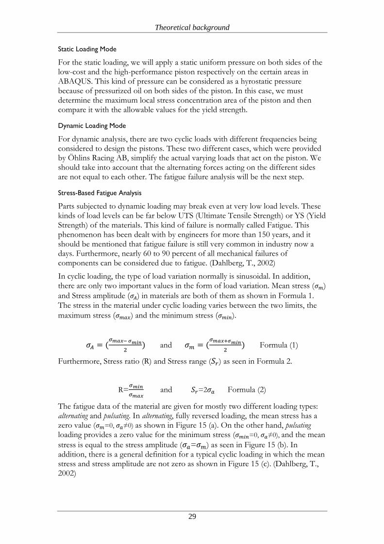
Based on the experiments, it seems just in the elastic region (no plastic deformations) the fatigue failure can be avoided. August Wöhler designed and developed the test machines as early as in 1858, and then carried out extensive series of fatigue test by controlling the applied load magnitude very carefully. According of those test series, the conclusion showed that there was a correlation between the fatigue life and the stress amplitude ( ) rather than the maximum stress. The fatigue life in stress cycles (N) can be plotted as a function of the
applied stress amplitude ( ). This graph is normally called a Wöhler or S-N (Stress-Number of cycles) curve as seen in Figure 16. (Dahlberg, T., 2002)
Figure 16. Wöhler or S-N curve.
Given stress..
σFL
σFL σUTS
Giv
es f
atig
ue
life
σUTS
N
S/𝜎𝐴
Giv
en f
atig
ue
life
Gives allowable stress..
101 10 103 104 1054 1064 1074
𝜎𝑎
−𝜎𝑎
𝜎
𝜎𝑚
𝜎𝑎
(a) (b) (c)
time
Theoretical background
31
As it can be shown from the above graph, the more fatigue life increases, the less stress amplitude is. In this logarithmic plot, the relation between fatigue life and stress amplitude is almost linear for a large portion in the form of a function as shown in Formula 3. Furthermore, the fatigue limit or sometimes endurance limit
stress as called is where no fatigue failure occurs. (Dahlberg, T., 2002)
=A logN+B Formula (3)
A & B are some parameters of material can be derived from the fatigue test.
However, in some cases when both axes for the stress amplitude ( ) and the number of cycles (N) are plotted in logarithm, a linear relation between them can be determined that may fit better to the experimental fatigue data as shown in Formula 4. (Dahlberg, T., 2002)
.N=K Formula (4)
As can be seen in the above-mentioned formula, m and K are material factors (determined from the fatigue tests).
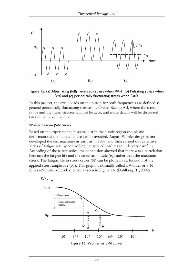
As already discussed, some materials never fail below the fatigue limit level ( ) as shown in Figure 17 (a) while the fatigue failure may occur for other materials
even at very low stress level as (b) in Figure 17. Thus, the fatigue strength ( )
would be defined for the stress amplitude level ( ) for a specified number of cycles of fatigue life (N) at which a test specimen or real structure may have as shown in Figure 17. Fatigue Strength can be also called Endurance Limit for N number of cycles. (Dahlberg, T., 2002)
Figure 17. Wöhler or S-N diagram for two main groups of materials. Curve (a) could
be defined as Steel and the other one (b) for Aluminium.
(a)
(b)
𝜎𝐴
𝜎𝑁
𝜎𝐹𝐿
101 10 103 104 1054 1064 1074
N
Theoretical background
32
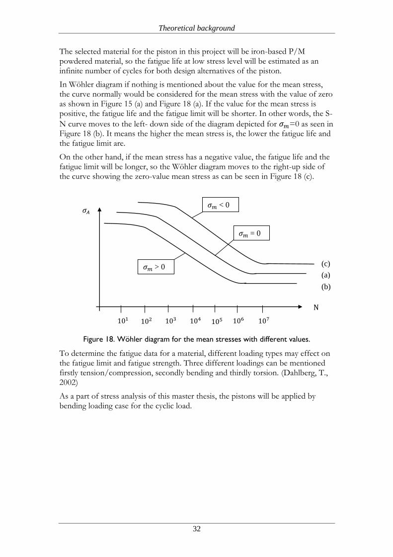
The selected material for the piston in this project will be iron-based P/M powdered material, so the fatigue life at low stress level will be estimated as an infinite number of cycles for both design alternatives of the piston.
In Wöhler diagram if nothing is mentioned about the value for the mean stress, the curve normally would be considered for the mean stress with the value of zero as shown in Figure 15 (a) and Figure 18 (a). If the value for the mean stress is positive, the fatigue life and the fatigue limit will be shorter. In other words, the S-
N curve moves to the left- down side of the diagram depicted for =0 as seen in Figure 18 (b). It means the higher the mean stress is, the lower the fatigue life and the fatigue limit are.
On the other hand, if the mean stress has a negative value, the fatigue life and the fatigue limit will be longer, so the Wöhler diagram moves to the right-up side of the curve showing the zero-value mean stress as can be seen in Figure 18 (c).
Figure 18. Wöhler diagram for the mean stresses with different values.
To determine the fatigue data for a material, different loading types may effect on the fatigue limit and fatigue strength. Three different loadings can be mentioned firstly tension/compression, secondly bending and thirdly torsion. (Dahlberg, T., 2002)
As a part of stress analysis of this master thesis, the pistons will be applied by bending loading case for the cyclic load.
(a)
(b)
101 10 103 104 1054 1064 1074
N
𝜎𝐴
(c) 𝜎𝑚 > 0
𝜎𝑚 < 0
𝜎𝑚 = 0
Theoretical background
33
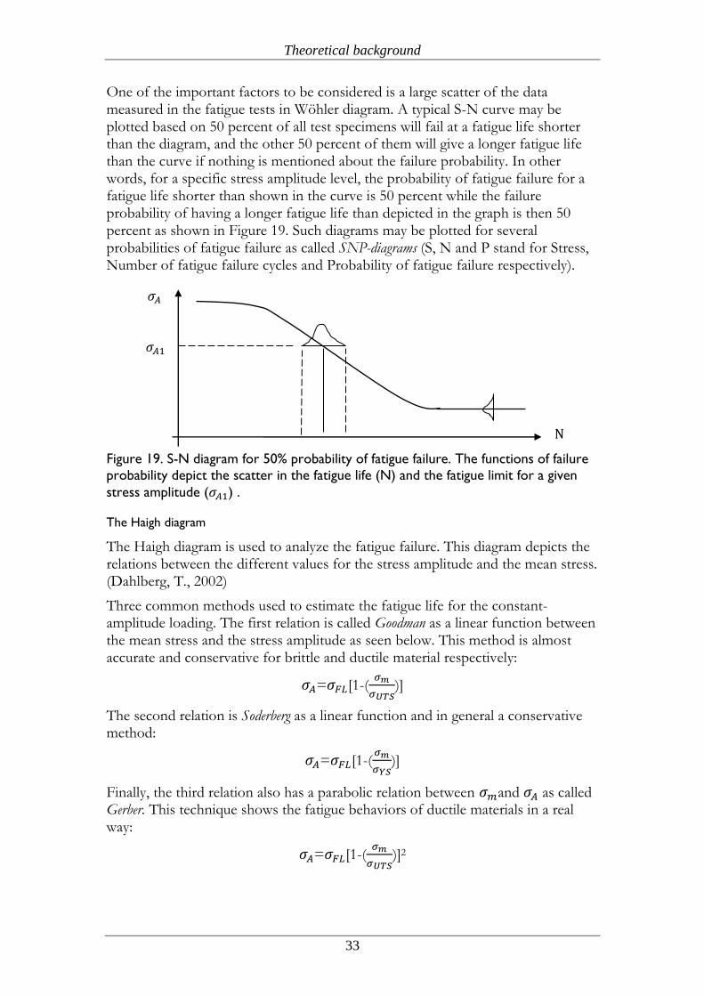
One of the important factors to be considered is a large scatter of the data measured in the fatigue tests in Wöhler diagram. A typical S-N curve may be plotted based on 50 percent of all test specimens will fail at a fatigue life shorter than the diagram, and the other 50 percent of them will give a longer fatigue life than the curve if nothing is mentioned about the failure probability. In other words, for a specific stress amplitude level, the probability of fatigue failure for a fatigue life shorter than shown in the curve is 50 percent while the failure probability of having a longer fatigue life than depicted in the graph is then 50 percent as shown in Figure 19. Such diagrams may be plotted for several probabilities of fatigue failure as called SNP-diagrams (S, N and P stand for Stress, Number of fatigue failure cycles and Probability of fatigue failure respectively).
Figure 19. S-N diagram for 50% probability of fatigue failure. The functions of failure
probability depict the scatter in the fatigue life (N) and the fatigue limit for a given
stress amplitude ( 1) .
The Haigh diagram
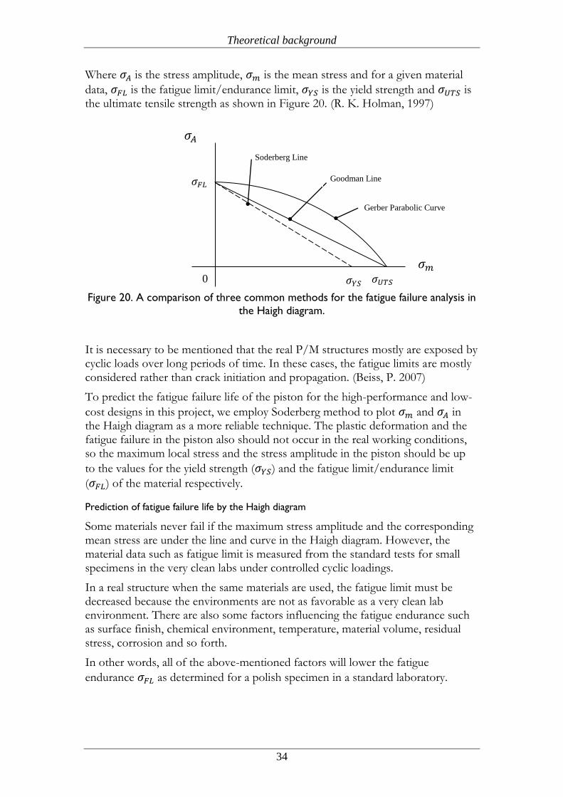
The Haigh diagram is used to analyze the fatigue failure. This diagram depicts the relations between the different values for the stress amplitude and the mean stress. (Dahlberg, T., 2002)
Three common methods used to estimate the fatigue life for the constant-amplitude loading. The first relation is called Goodman as a linear function between the mean stress and the stress amplitude as seen below. This method is almost accurate and conservative for brittle and ductile material respectively:
= [1-(
)]
The second relation is Soderberg as a linear function and in general a conservative method:
= [1-(
)]
Finally, the third relation also has a parabolic relation between and as called Gerber. This technique shows the fatigue behaviors of ductile materials in a real way:
= [1-(
)]2
N
𝜎𝐴
𝜎𝐴1
Theoretical background
34
Where is the stress amplitude, is the mean stress and for a given material
data, is the fatigue limit/endurance limit, is the yield strength and is the ultimate tensile strength as shown in Figure 20. (R. K. Holman, 1997)
Figure 20. A comparison of three common methods for the fatigue failure analysis in
the Haigh diagram.
It is necessary to be mentioned that the real P/M structures mostly are exposed by cyclic loads over long periods of time. In these cases, the fatigue limits are mostly considered rather than crack initiation and propagation. (Beiss, P. 2007)
To predict the fatigue failure life of the piston for the high-performance and low-
cost designs in this project, we employ Soderberg method to plot and in the Haigh diagram as a more reliable technique. The plastic deformation and the fatigue failure in the piston also should not occur in the real working conditions, so the maximum local stress and the stress amplitude in the piston should be up
to the values for the yield strength ( ) and the fatigue limit/endurance limit
( ) of the material respectively.
Prediction of fatigue failure life by the Haigh diagram
Some materials never fail if the maximum stress amplitude and the corresponding mean stress are under the line and curve in the Haigh diagram. However, the material data such as fatigue limit is measured from the standard tests for small specimens in the very clean labs under controlled cyclic loadings.
In a real structure when the same materials are used, the fatigue limit must be decreased because the environments are not as favorable as a very clean lab environment. There are also some factors influencing the fatigue endurance such as surface finish, chemical environment, temperature, material volume, residual stress, corrosion and so forth.
In other words, all of the above-mentioned factors will lower the fatigue
endurance as determined for a polish specimen in a standard laboratory.
0
𝜎𝐴
𝜎𝑚
𝜎𝐹𝐿
𝜎𝑌𝑆 𝜎𝑈𝑇𝑆
Gerber Parabolic Curve
Goodman Line
Soderberg Line
Theoretical background
35
The surface finish factor even on a polished part can reduce the fatigue endurance
( ). A rough surface on a component can cause stress concentration at the irregularities on surface, and consequently it can make the fatigue cracks start
propagating easily on the uneven surface. This factor is denoted by (kappa).
The other factor is called (Lambda) for the material volume/size. All material data are gathered from a test specimen with a standard size (Dim. 10 mm). For real components or bigger specimens, the fatigue limit will be reduced because of higher probabilities of finding a discontinuity, irregularities, inclusions, defects and so forth for a fatigue crack to initiate and propagate in a whole mass. Thus, the larger the structure is in size, the lower the fatigue limit is in comparison with the fatigue endurance measured from a standard test specimen in a lab. It is necessary to be mentioned that the volume of raw material should be considered not the volume of the final component.
The (delta) is another factor for the loaded volume will be put on the list of reducing factors in calculating of the real fatigue limit. This factor is defined to reduce the fatigue limit only for the specimens or structures loaded by cyclic bending/torsion where the stress ingredient is present. It is supposed to be taken into consideration that in a larger structure/specimen there is higher probability of existing defects, inclusions, and discontinuities to make fatigue cracks initiate and grow faster than in a normal test specimen. For the tension/compression loading,
the value for (delta) will be one ( =1). (Dahlberg, T., 2002)
In some other references the value of load factor for bending loading also refers to one. (Marghitu, D. B., 2001)
The material behavior in some standard experiments shows greater fatigue strength under bending loading that axial loading. During applying the bending load, the stress gradients in the components are quite steeper, so the most maximum stressed volume of material may get smaller. In this case, the probability of failure will be considerably reduced because the lower number of defects in that smaller material volume in which failure may occur gets involved. (Sonsino, C. M., 1994)
After determining all three factors, the fatigue limit for both the alternating and
the pulsating cyclic loadings should be multiplied by the coefficient of . . as the followings:
. . . Reduced
The reduced fatigue limit will be plotted in the High diagram.
However, there are some other factors can influence the fatigue limit such as temperature in a real working condition, chemical environment, welding and so forth.
Theoretical background
36
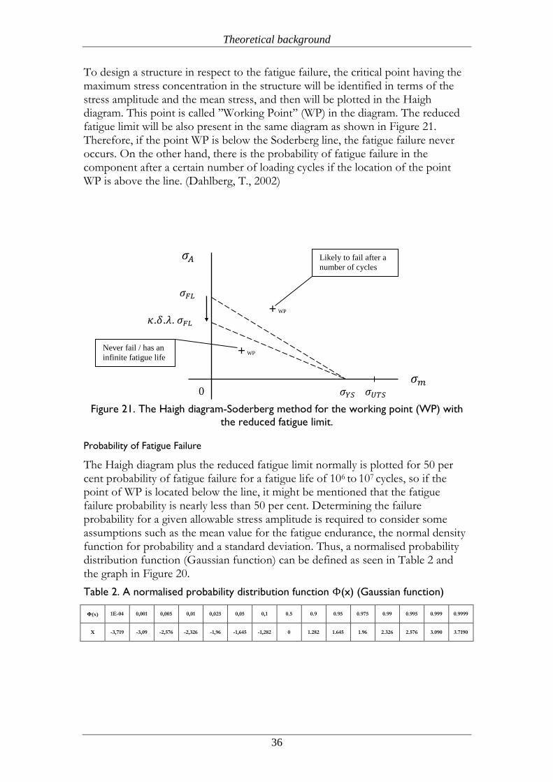
To design a structure in respect to the fatigue failure, the critical point having the maximum stress concentration in the structure will be identified in terms of the stress amplitude and the mean stress, and then will be plotted in the Haigh diagram. This point is called ’’Working Point’’ (WP) in the diagram. The reduced fatigue limit will be also present in the same diagram as shown in Figure 21. Therefore, if the point WP is below the Soderberg line, the fatigue failure never occurs. On the other hand, there is the probability of fatigue failure in the component after a certain number of loading cycles if the location of the point WP is above the line. (Dahlberg, T., 2002)
Figure 21. The Haigh diagram-Soderberg method for the working point (WP) with
the reduced fatigue limit.
Probability of Fatigue Failure
The Haigh diagram plus the reduced fatigue limit normally is plotted for 50 per cent probability of fatigue failure for a fatigue life of 106 to 107 cycles, so if the point of WP is located below the line, it might be mentioned that the fatigue failure probability is nearly less than 50 per cent. Determining the failure probability for a given allowable stress amplitude is required to consider some assumptions such as the mean value for the fatigue endurance, the normal density function for probability and a standard deviation. Thus, a normalised probability distribution function (Gaussian function) can be defined as seen in Table 2 and the graph in Figure 20.
Table 2. A normalised probability distribution function (x) (Gaussian function)
(x) 1E-04 0,001 0,005 0,01 0,025 0,05 0,1 0.5 0.9 0.95 0.975 0.99 0.995 0.999 0.9999
X -3,719 -3,09 -2,576 -2,326 -1,96 -1,645 -1,282 0 1.282 1.645 1.96 2.326 2.576 3.090 3.7190
0
𝜎𝐴
𝜎𝑚
𝜎𝐹𝐿
𝜎𝑌𝑆 𝜎𝑈𝑇𝑆
𝜅.𝛿.𝜆. 𝜎𝐹𝐿
+ WP
+ WP
Likely to fail after a
number of cycles
Never fail / has an
infinite fatigue life
Theoretical background
37
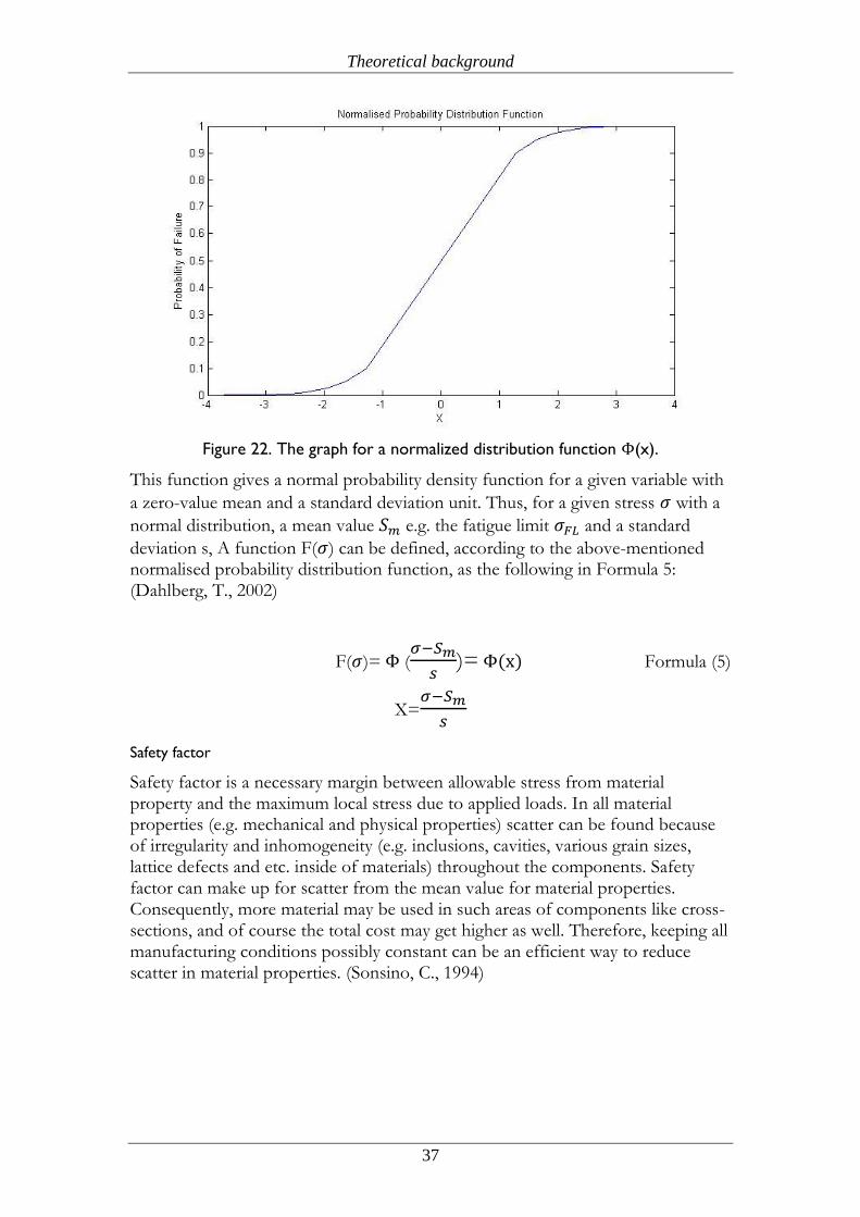
Figure 22. The graph for a normalized distribution function (x).
This function gives a normal probability density function for a given variable with
a zero-value mean and a standard deviation unit. Thus, for a given stress with a
normal distribution, a mean value e.g. the fatigue limit and a standard
deviation s, A function F( ) can be defined, according to the above-mentioned normalised probability distribution function, as the following in Formula 5: (Dahlberg, T., 2002)
F( )= (
)= Formula (5)
X=
Safety factor
Safety factor is a necessary margin between allowable stress from material property and the maximum local stress due to applied loads. In all material properties (e.g. mechanical and physical properties) scatter can be found because of irregularity and inhomogeneity (e.g. inclusions, cavities, various grain sizes, lattice defects and etc. inside of materials) throughout the components. Safety factor can make up for scatter from the mean value for material properties. Consequently, more material may be used in such areas of components like cross-sections, and of course the total cost may get higher as well. Therefore, keeping all manufacturing conditions possibly constant can be an efficient way to reduce scatter in material properties. (Sonsino, C., 1994)
Theoretical background
38
For P/M steel components, the scatter of the fatigue strength ( ) is not greater that wrought steels, but less than welded and cast iron parts for a given batch. Other scatters may be considerably observed if the important parameters of P/M manufacturing process (e.g. sintering time/temperature, compacting pressure, chemical composition and etc.) are not controlled in a structured way. However, the results from test samples (produced by different manufacturers under very well-controlled production conditions) show less scatters and more reliable structures.
According to the normalised probability distribution function (x) (Gaussian function) in the above-mentioned part (Figure 22 and Table 2)and the experience, the safety factor can be determined by calculating different scatters
(S S S ) and probability of failure ( ). Formula 6 mentioned below is shown the safety factor as a function of various variables as the followings: (Sonsino, C., 1994)
N= 10 Formula (6)
Where S=√
And =0.39 * log (1/ ) and = 1:
N= Safety factor,
S = the standard derivation of the cyclic loading,
S = the standard derivation of the mean value for the strength, e.g. in a given batch,
S = the standard derivation for the fluctuation of the mean value, e.g. within several batches,
X= a relative- dependent variable on the probability of failure ( ), e.g. can be
calculated by using Table 2 for a given ,
Then, allowable local stress (.e.g. for the fatigue endurance at of 50%) may be determined to be divided by N as shown in Formula 7:
Allowable = (
) Formula (7)
2.6.3 Element Selection
Element selection is an important part of a finite element simulation. One should be aware of the advantages and disadvantages of the element at hand in order not to misinterpret the results.
Theoretical background
39
ABAQUS offers a variety of choices when it comes to elements, most common being linear/quadratic hexahedral and linear/quadratic tetrahedral elements. It is known that hexahedral elements hold an advantage over tetrahedral elements in terms of accuracy, reliability and reduced errors. However, hexahedral elements can be extremely time consuming and hard to establish on complex models, whereas tetrahedral elements are easy to automate and can be applied readily on very complex geometries in relatively shorter times. There are some algorithms available that can create more than 400,000 tetrahedrons per minute. But concerning hexahedral mesh algorithms this is not the case. (Shepherd, 2008)
Hexahedral meshes can be built only on specific geometries. Thus, the model to be analysed should be cut down into smaller sections, on which hexahedral meshes can be generated. This operation of cutting the model into smaller pieces, which is also called partitioning, can be extremely time consuming, taking up to several months for generalized models. Tetrahedral meshes in this regard have a significant advantage over hexahedral meshes. The same operation for tetrahedral meshes might take only hours or days to accomplish. (Shepherd, 2008)
However, despite this disadvantage, sometimes hexahedral meshes can be preferred over tetrahedral meshes because of some reasons. First of all, in order to get a similar level of accuracy and reliability, number of elements in a tetrahedral mesh model should be 4-10 times the number of hexahedral model. This will increase the simulation time. Moreover, in some applications tetrahedral elements will be stiffer because of reduced number of degrees of freedom associated with tetrahedral elements. This is called tet-locking or mesh-locking and it may lead us to interpret the results in a wrong way (Shepherd, 2008).
However, there has been some research which suggested that quadratic tetrahedral elements showed equal performance compared to bilinear hexahedral elements with respect to accuracy and computational time. (Cifuentes, 1992)
Wang et. Al. Simulated a beam fixed on one end and loaded on the other end. They compared the experimental results with the numerical results. It was found that quadratic tetrahedral and quadradic hexahedral elements gave very close results to the experimental results. Linear tetrahedral elements, on the other hand, were less accurate (Wang, 2004). Cifuentes et. Al also used the same model to compare the processing times of different elements. They found out that quadratic tetrahedral and linear hexahedral elements exhibit same results in accuracy and processing time. (Cifuentes, 1992)
In another research, Veyhl et al did a study on a beam with a square, a circular and a rail section with tetrahedral, hexahedral, mixed and voxel meshes. They found out that mixed meshes (tetrahedral and hexahedral) exhibit the most accurate results compared to other type of elements. Linear hexahedral elements gave also good results, while tetrahedral elements resulted in the biggest deviation from the analytical results. However, with the increasing number of nodes, tetrahedral elements showed closer results to those of hexahedral elements. (Veyhl, 2010)
Theoretical background
40
Benzley et. al conducted an experiment with a beam model fixed on one end, subjected to bending and torsional load respectively. They used linear tetrahedron, quadratic tetrahedron, linear hexahedron and quadratic hexahedron elements and compared the results. They found out that in both types of loading, linear tetrahedron gave the biggest error compared to analytical solutions. Linear hexahedron was better comparing to linear tetrahedron. Both quadratic elements showed more or less the same performance and both were much closer to analytical solution than linear hexahedron. In the elastoplastic experiment with same model and same elements, linear tetrahedron elements showed again the worst performance and did not even initiate plasticity when it was supposed to, according to the analytical solution. Quadratic elements of both hexahedron and tetrahedron showed acceptable performance, however, giving bigger error comparing to elastic experiment. (Benzley, 1995)
Method
41
3 Method
Before starting to develop the piston form the base-design to the final product through the whole process of product development, it is crucial to set the methodology and then the requirements properly and keep them in mind throughout the product development process.
3.1 Product Development Methodology
A few components still are designed and developed by some trial & error methods nowadays. Instead, the modern and systematic product development methods facilitate this process for designers to develop the components by the efficient and modern tools such as CAD (Computer-Aided Design) for 3D modelling , FEM (Finite Element Method) for analysis, CES (Cambridge Engineering Software) for material & manufacturing process selection, CAM (Computer-Aided Manufacturing) for simulating the manufacturing processes and etc. To implement this project, the following stages as a product development procedure will be applied:
3.1.1 Load Calculation and Assessment
Load calculation is considered as the most important part of the whole product development methods. It actually influences the material/manufacturing method selection and geometrical dimensions of components especially for the structural parts. The load should be calculated and assessed very carefully by measuring the load from similar components or calculating and determining the real load, regarding the necessary assumptions and considerations such as the risk factors, standards, safety margins and so forth. The final results of this stage will have a strong effect on the next stages. (Sonsino, C. M., 1994)
3.1.2 Dimensional Geometry of Component & Structural Parts
Before modelling the three-dimensional geometrical shape of a component, some factors should be taken into consideration. Geometrical constraints, dimensional simplicity, functionality of the component (especially with other attached components), manufacturability (manufacturing process should be selected as simple and cheap as possible), material selection (meeting the main requirements), cost efficiency (analysis, design and manufacture cost), weight (less material & lighter material) and environmental issues (e.g. lower energy-consumption) can be kept in mind as some of those important factors in this stage.
Method
42
3.1.3 Material and manufacturing process selection
After the second stage in the product development procedure, it is time to select the material and manufacturing method efficiently and economically. The production rate can be the most important factor in determining the best choice of material and manufacturing method. The tooling, labour, energy and other costs can be considered to come up with the final decision for the manufacturing process. In addition, appropriate material (considering mechanical and physical properties) is selected based on meeting the requirements such as fulfilment of loads, cheaper price, environmental-friendly, safety issues, longer cycle life, recyclability, and other issues. In this step, an optimal point may be determined by comparing and selecting between various materials and manufacturing processes in terms of all above-mentioned factors.
3.1.4 Stress Analysis
Determination of the maximum local stresses and critical areas of loaded structural parts is the main task of this stage. Almost all components have geometrical irregularities like reduction of cross sectional areas or different forms of geometrical features which they are considered as stress raisers and notches. Consequently, design engineers must focus on them to find out the distribution of maximum local stresses and the most critical areas of the part. Furthermore, they should not exceed the maximum allowable stress of material in order not to fail in working conditions. This job can be done by FEM methods.
In this project, ABAQUS will be used to analyse the stresses while the piston is loaded by two different loads, static and cyclic.
3.1.5 Allowable Local Stresses
The allowable local stresses are a part of mechanical properties of materials measured by carrying out the standard test on specimens or structural parts. Then, scatter and other factors must be also considered to determine the allowable local stresses of the parts. They are mostly material-dependent, and some of them can be derived from the manufacturing methods, load scatter, surface finish, stress concentration factors, safety margins, loaded volume and so forth.
3.1.6 Comparison of Stresses
In this stage, the aim is to compare the maximum local stress with allowable local stress in the structural part. The final design can be considered as safe if the maximum local stress does not exceed the allowable local stress. Otherwise, there are two other results, first the failure may occur if the maximum local stress is more that allowable local stress, second the optimal design can be determined if they equal to each other.

Method
43
3.1.7 Testing and Verification
The final step of the whole product development process is to test and verify the prototype of the part. The purpose is to make sure whether the part is designed properly and safely. Regarding the related standards, making prototype and getting it tested under the service loading may be verified in the simulated real working conditions in the lab. (Sonsino, C. M., 1994)
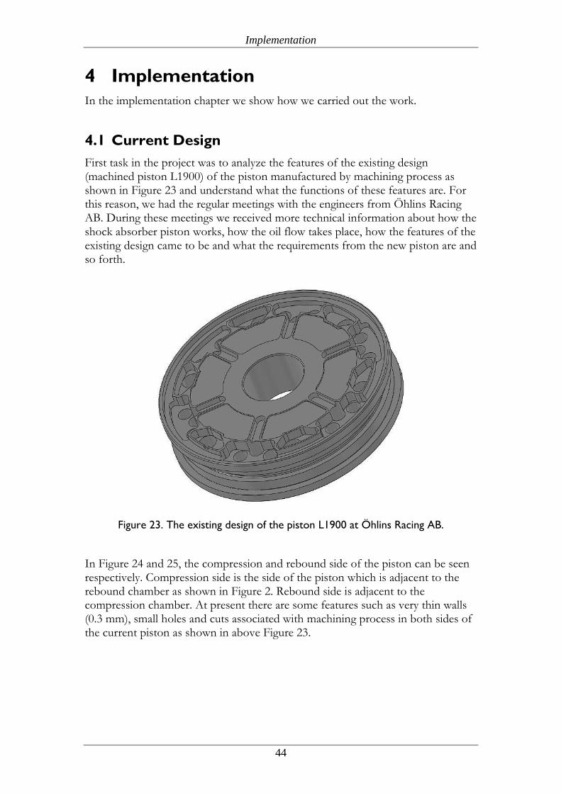
Implementation
44
4 Implementation
In the implementation chapter we show how we carried out the work.
4.1 Current Design
First task in the project was to analyze the features of the existing design (machined piston L1900) of the piston manufactured by machining process as shown in Figure 23 and understand what the functions of these features are. For this reason, we had the regular meetings with the engineers from Öhlins Racing AB. During these meetings we received more technical information about how the shock absorber piston works, how the oil flow takes place, how the features of the existing design came to be and what the requirements from the new piston are and so forth.
Figure 23. The existing design of the piston L1900 at Öhlins Racing AB.
In Figure 24 and 25, the compression and rebound side of the piston can be seen respectively. Compression side is the side of the piston which is adjacent to the rebound chamber as shown in Figure 2. Rebound side is adjacent to the compression chamber. At present there are some features such as very thin walls (0.3 mm), small holes and cuts associated with machining process in both sides of the current piston as shown in above Figure 23.
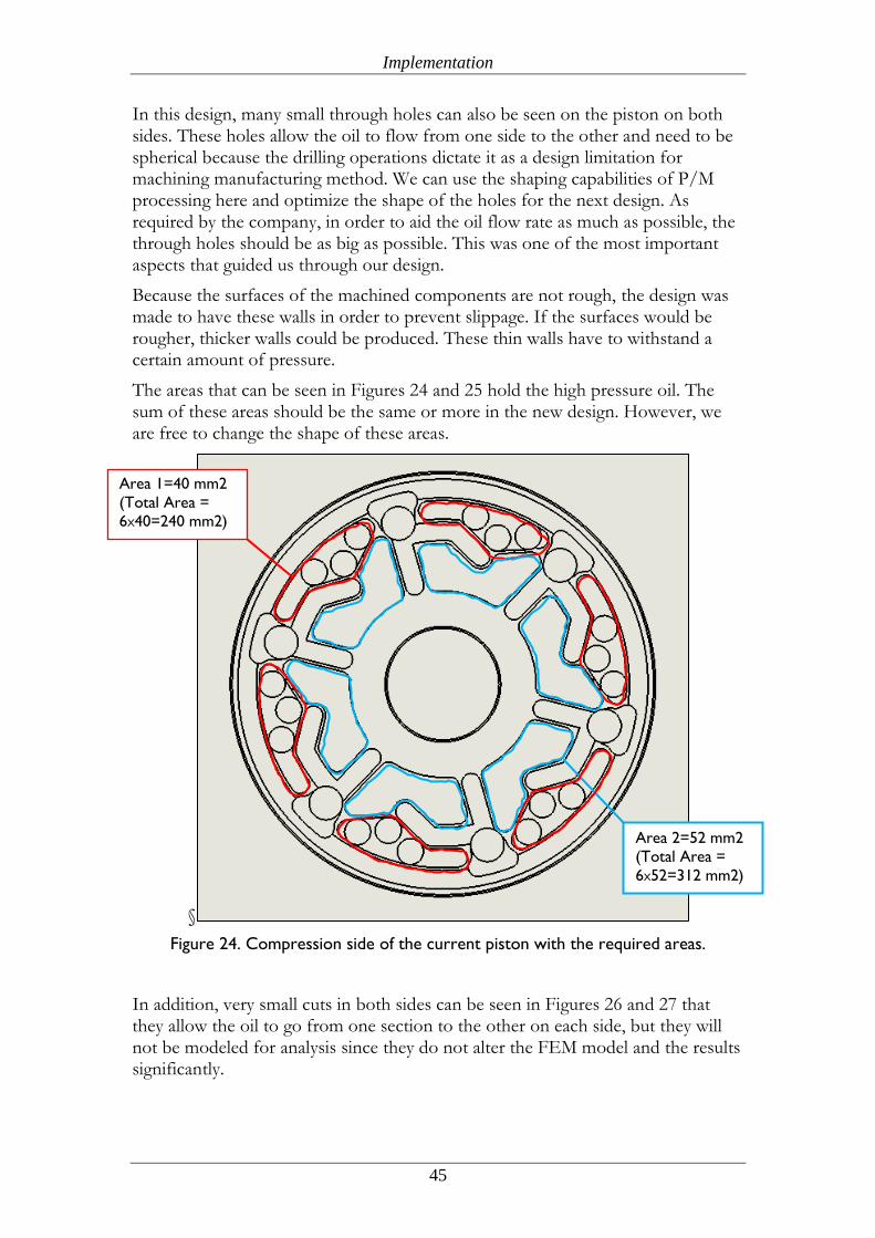
Implementation
45
In this design, many small through holes can also be seen on the piston on both sides. These holes allow the oil to flow from one side to the other and need to be spherical because the drilling operations dictate it as a design limitation for machining manufacturing method. We can use the shaping capabilities of P/M processing here and optimize the shape of the holes for the next design. As required by the company, in order to aid the oil flow rate as much as possible, the through holes should be as big as possible. This was one of the most important aspects that guided us through our design.
Because the surfaces of the machined components are not rough, the design was made to have these walls in order to prevent slippage. If the surfaces would be rougher, thicker walls could be produced. These thin walls have to withstand a certain amount of pressure.
The areas that can be seen in Figures 24 and 25 hold the high pressure oil. The sum of these areas should be the same or more in the new design. However, we are free to change the shape of these areas.
§
Figure 24. Compression side of the current piston with the required areas.
In addition, very small cuts in both sides can be seen in Figures 26 and 27 that they allow the oil to go from one section to the other on each side, but they will not be modeled for analysis since they do not alter the FEM model and the results significantly.
Area 1=40 mm2
(Total Area =
6X40=240 mm2)
Area 2=52 mm2
(Total Area =
6X52=312 mm2)
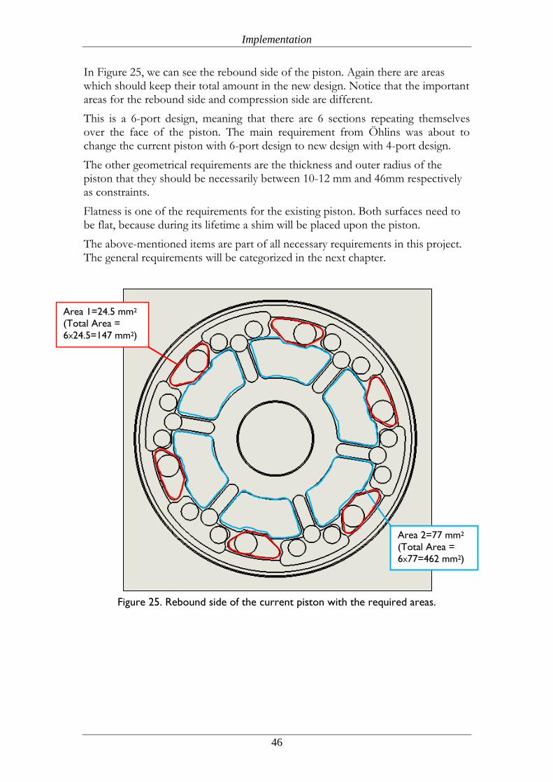
Implementation
46
In Figure 25, we can see the rebound side of the piston. Again there are areas which should keep their total amount in the new design. Notice that the important areas for the rebound side and compression side are different.
This is a 6-port design, meaning that there are 6 sections repeating themselves over the face of the piston. The main requirement from Öhlins was about to change the current piston with 6-port design to new design with 4-port design.
The other geometrical requirements are the thickness and outer radius of the piston that they should be necessarily between 10-12 mm and 46mm respectively as constraints.
Flatness is one of the requirements for the existing piston. Both surfaces need to be flat, because during its lifetime a shim will be placed upon the piston.
The above-mentioned items are part of all necessary requirements in this project. The general requirements will be categorized in the next chapter.
Figure 25. Rebound side of the current piston with the required areas.
Area 1=24.5 mm2
(Total Area =
6X24.5=147 mm2)
Area 2=77 mm2
(Total Area =
6X77=462 mm2)
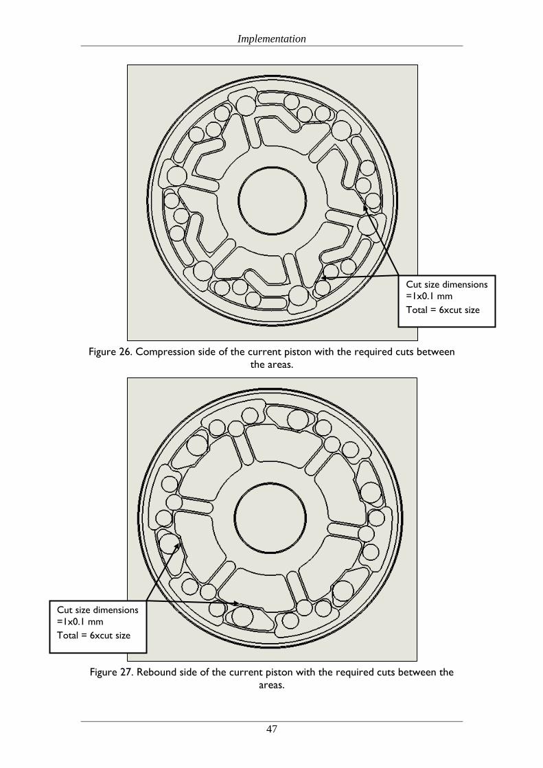
Implementation
47
Figure 26. Compression side of the current piston with the required cuts between
the areas.
Figure 27. Rebound side of the current piston with the required cuts between the
areas.
Cut size dimensions
=1x0.1 mm
Total = 6xcut size
Cut size dimensions
=1x0.1 mm
Total = 6xcut size
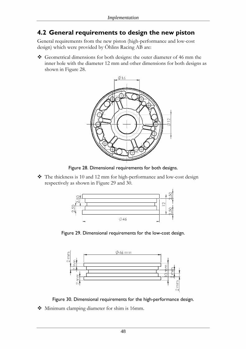
Implementation
48
4.2 General requirements to design the new piston
General requirements from the new piston (high-performance and low-cost design) which were provided by Öhlins Racing AB are:
Geometrical dimensions for both designs: the outer diameter of 46 mm the inner hole with the diameter 12 mm and other dimensions for both designs as shown in Figure 28.
Figure 28. Dimensional requirements for both designs.
The thickness is 10 and 12 mm for high-performance and low-cost design respectively as shown in Figure 29 and 30.
Figure 29. Dimensional requirements for the low-cost design.
Figure 30. Dimensional requirements for the high-performance design.
Minimum clamping diameter for shim is 16mm.
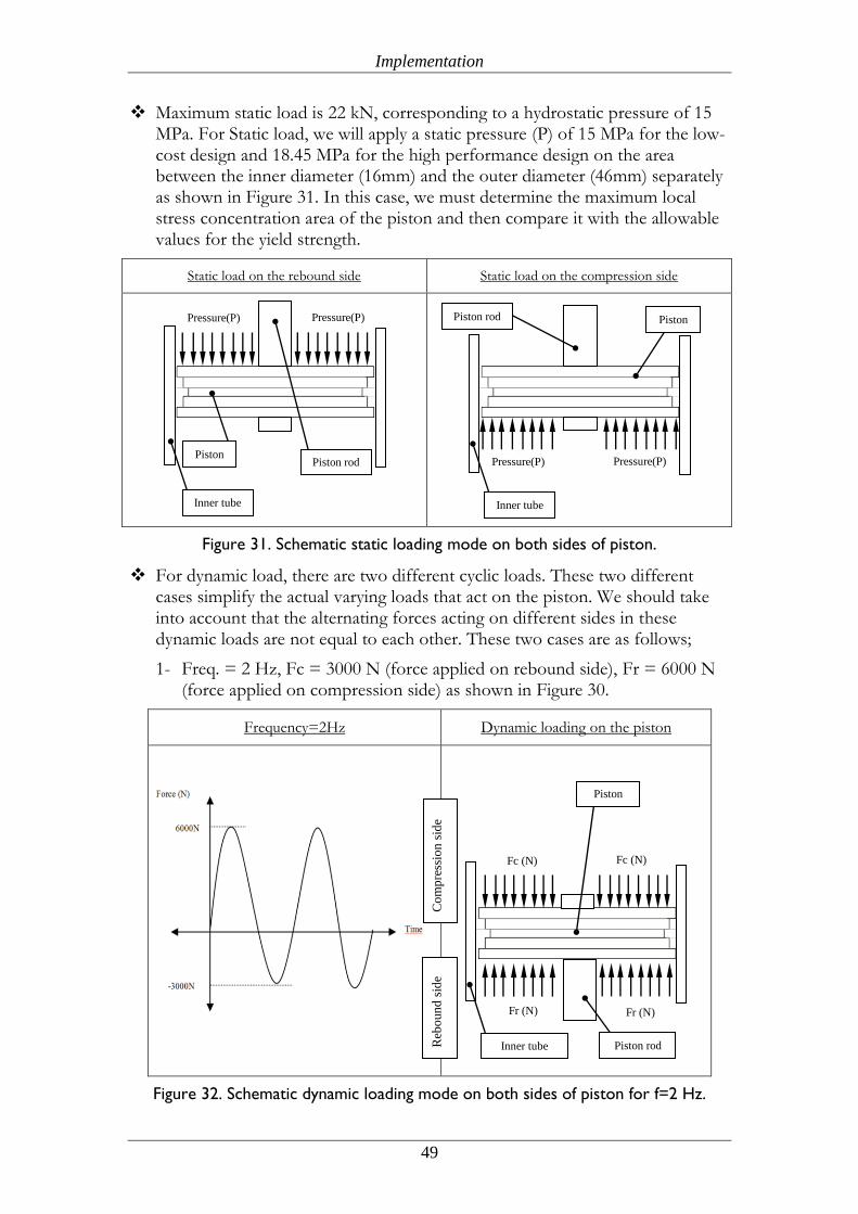
Implementation
49
Maximum static load is 22 kN, corresponding to a hydrostatic pressure of 15 MPa. For Static load, we will apply a static pressure (P) of 15 MPa for the low-cost design and 18.45 MPa for the high performance design on the area between the inner diameter (16mm) and the outer diameter (46mm) separately as shown in Figure 31. In this case, we must determine the maximum local stress concentration area of the piston and then compare it with the allowable values for the yield strength.
Static load on the rebound side Static load on the compression side
Figure 31. Schematic static loading mode on both sides of piston.
For dynamic load, there are two different cyclic loads. These two different cases simplify the actual varying loads that act on the piston. We should take into account that the alternating forces acting on different sides in these dynamic loads are not equal to each other. These two cases are as follows;
1- Freq. = 2 Hz, Fc = 3000 N (force applied on rebound side), Fr = 6000 N (force applied on compression side) as shown in Figure 30.
Frequency=2Hz Dynamic loading on the piston
Figure 32. Schematic dynamic loading mode on both sides of piston for f=2 Hz.
Piston Piston rod
Pressure(P) Pressure(P)
Inner tube
Piston rod Piston
Pressure(P) Pressure(P)
Inner tube
Piston
rod
Fr (N)
Inner tube
Co
mp
ress
ion
sid
e R
ebo
un
d s
ide
Fr (N)
Fc (N) Fc (N)
Piston rod
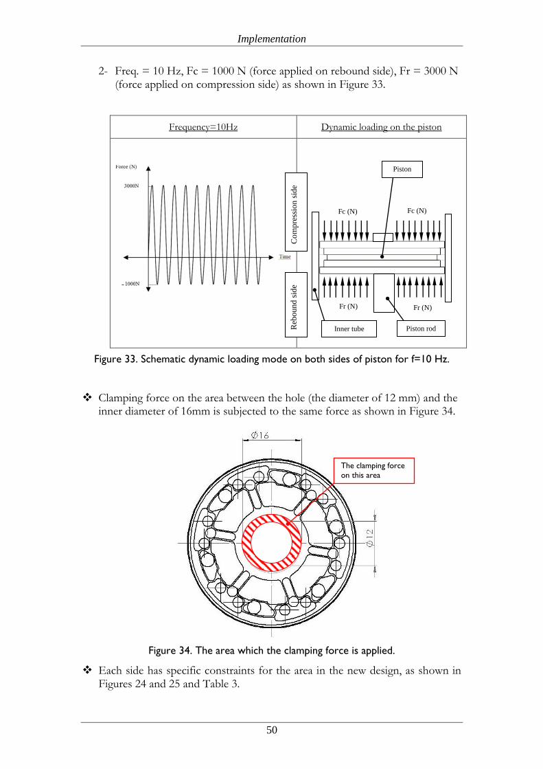
Implementation
50
2- Freq. = 10 Hz, Fc = 1000 N (force applied on rebound side), Fr = 3000 N (force applied on compression side) as shown in Figure 33.
Frequency=10Hz Dynamic loading on the piston
Figure 33. Schematic dynamic loading mode on both sides of piston for f=10 Hz.
Clamping force on the area between the hole (the diameter of 12 mm) and the inner diameter of 16mm is subjected to the same force as shown in Figure 34.
Figure 34. The area which the clamping force is applied.
Each side has specific constraints for the area in the new design, as shown in Figures 24 and 25 and Table 3.
Piston
rod
Fr (N)
Inner tube
Co
mp
ress
ion
sid
e R
ebo
un
d s
ide
Fr (N)
Fc (N) Fc (N)
Piston rod
The clamping force
on this area
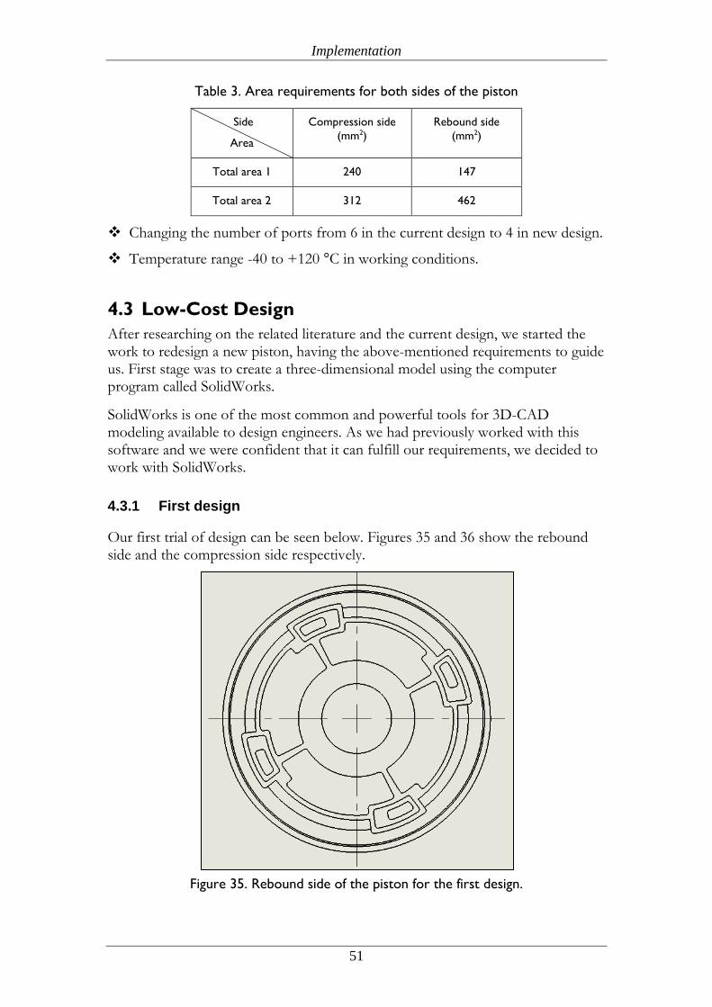
Implementation
51
Table 3. Area requirements for both sides of the piston
Side
Area
Compression side
(mm2)
Rebound side
(mm2)
Total area 1 240 147
Total area 2 312 462
Changing the number of ports from 6 in the current design to 4 in new design.
Temperature range -40 to +120 C in working conditions.
4.3 Low-Cost Design
After researching on the related literature and the current design, we started the work to redesign a new piston, having the above-mentioned requirements to guide us. First stage was to create a three-dimensional model using the computer program called SolidWorks.
SolidWorks is one of the most common and powerful tools for 3D-CAD modeling available to design engineers. As we had previously worked with this software and we were confident that it can fulfill our requirements, we decided to work with SolidWorks.
4.3.1 First design
Our first trial of design can be seen below. Figures 35 and 36 show the rebound side and the compression side respectively.
Figure 35. Rebound side of the piston for the first design.
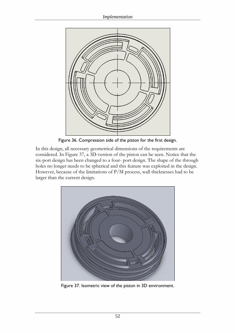
Implementation
52
Figure 36. Compression side of the piston for the first design.
In this design, all necessary geometrical dimensions of the requirements are considered. In Figure 37, a 3D-version of the piston can be seen. Notice that the six-port design has been changed to a four- port design. The shape of the through holes no longer needs to be spherical and this feature was exploited in the design. However, because of the limitations of P/M process, wall thicknesses had to be larger than the current design.
Figure 37. Isometric view of the piston in 3D environment.
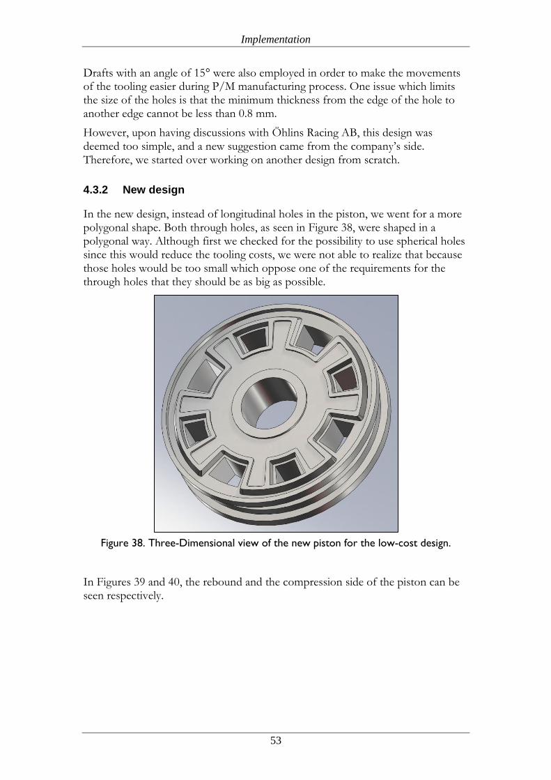
Implementation
53
Drafts with an angle of 15° were also employed in order to make the movements of the tooling easier during P/M manufacturing process. One issue which limits the size of the holes is that the minimum thickness from the edge of the hole to another edge cannot be less than 0.8 mm.
However, upon having discussions with Öhlins Racing AB, this design was deemed too simple, and a new suggestion came from the company’s side. Therefore, we started over working on another design from scratch.
4.3.2 New design
In the new design, instead of longitudinal holes in the piston, we went for a more polygonal shape. Both through holes, as seen in Figure 38, were shaped in a polygonal way. Although first we checked for the possibility to use spherical holes since this would reduce the tooling costs, we were not able to realize that because those holes would be too small which oppose one of the requirements for the through holes that they should be as big as possible.
Figure 38. Three-Dimensional view of the new piston for the low-cost design.
In Figures 39 and 40, the rebound and the compression side of the piston can be seen respectively.
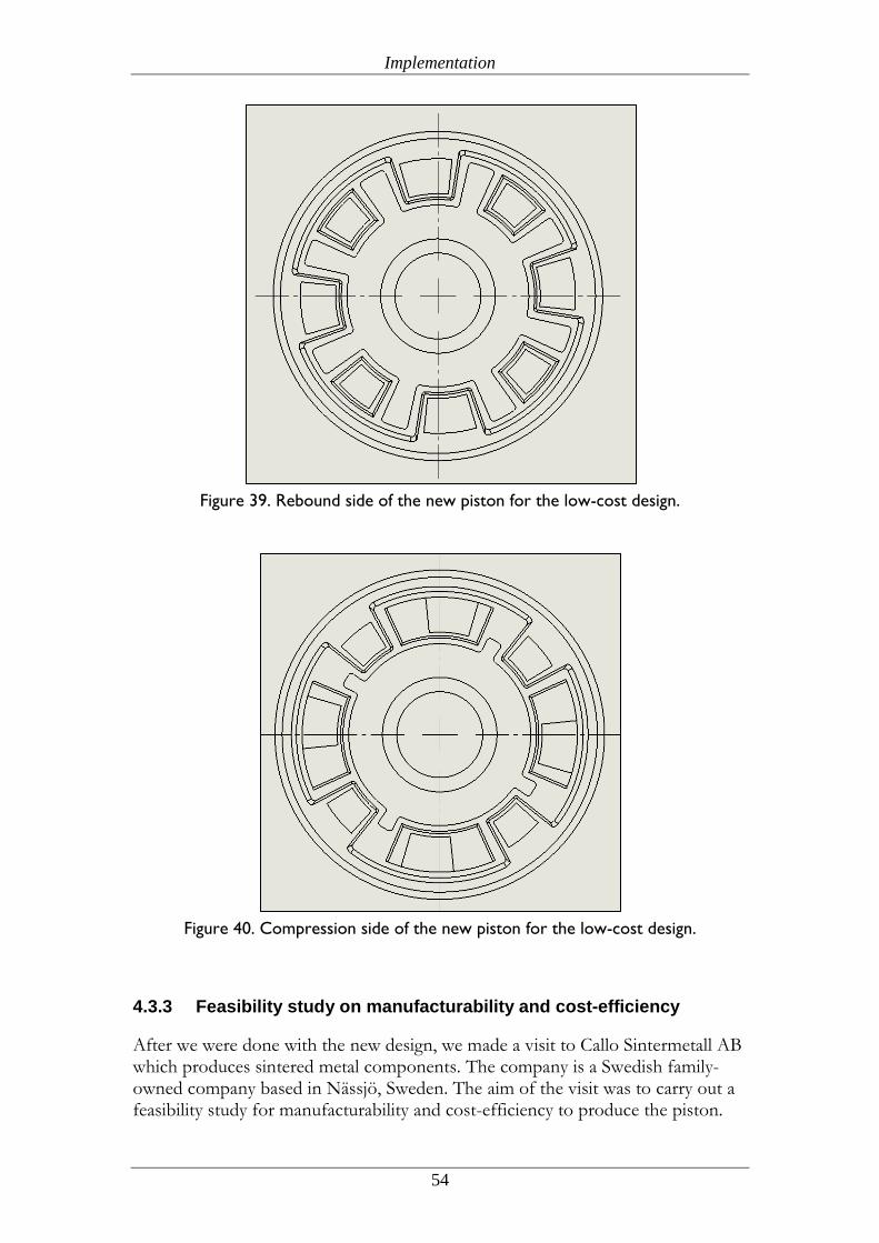
Implementation
54
Figure 39. Rebound side of the new piston for the low-cost design.
Figure 40. Compression side of the new piston for the low-cost design.
4.3.3 Feasibility study on manufacturability and cost-efficiency
After we were done with the new design, we made a visit to Callo Sintermetall AB which produces sintered metal components. The company is a Swedish family-owned company based in Nässjö, Sweden. The aim of the visit was to carry out a feasibility study for manufacturability and cost-efficiency to produce the piston.
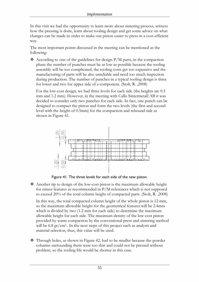
Implementation
55
In this visit we had the opportunity to learn more about sintering process, witness how the pressing is done, learn about tooling design and get some advice on what changes can be made in order to make our piston easier to press in a cost-efficient way.
The most important points discussed in the meeting can be mentioned as the following:
According to one of the guidelines for design P/M parts, in the compaction phase the number of punches must be as low as possible because the tooling assembly will be too complicated, the tooling costs get too expensive and the manufacturing of parts will be also unreliable and need too much inspection during production. The number of punches in a typical tooling design is three for lower and two for upper side of a component. (Stolt, R. ,2008)
For the low-cost design, we had three levels for each side (the heights are 0.5 mm and 1.2 mm). However, in the meeting with Callo Sintermetall AB it was decided to consider only two punches for each side. In fact, one punch can be designed to compact the piston and form the two levels (the first and second level with the height of 0.5mm) for the compaction and rebound side as shown in Figure 41.
Figure 41. The three levels for each side of the new piston.
Another tip to design of the low-cost piston is the maximum allowable height for minor features as recommended in P/M references which is not supposed to exceed 20% of the total column height of compacted parts. (Stolt, R. ,2008)
In this way, the total compacted column height of the whole piston is 12 mm, so the maximum allowable height for the geometrical features will be 2.4mm which is divided by two (1.2 mm for each side) to determine the maximum allowable height for each side. The maximum density of the low-cost piston provided by warm compaction by the conventional press and sintering method will be 6.8 gr/cm3 . In the next steps of this project such as analysis and material selection, thus, this value will be used.
Through holes, as shown in Figure 42, had to be smaller because the powder columns surrounding them were too thin and could not be pressed without problem, so the tooling life would be shorter in this case.
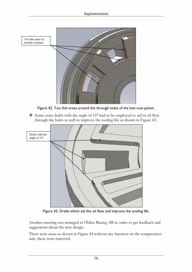
Implementation
56
Figure 42. Too thin areas around the through holes of the low-cost piston.
Some extra drafts with the angle of 15 had to be employed to aid in oil flow through the holes as well to improve the tooling life as shown in Figure 43.
Figure 43. Drafts which aid the oil flow and improve the tooling life.
Another meeting was arranged in Öhlins Racing AB in order to get feedback and suggestions about the new design.
There were areas as shown in Figure 44 without any function on the compression side, these were removed.
Too thin areas of
powder columns
Drafts with the
angle of 15°
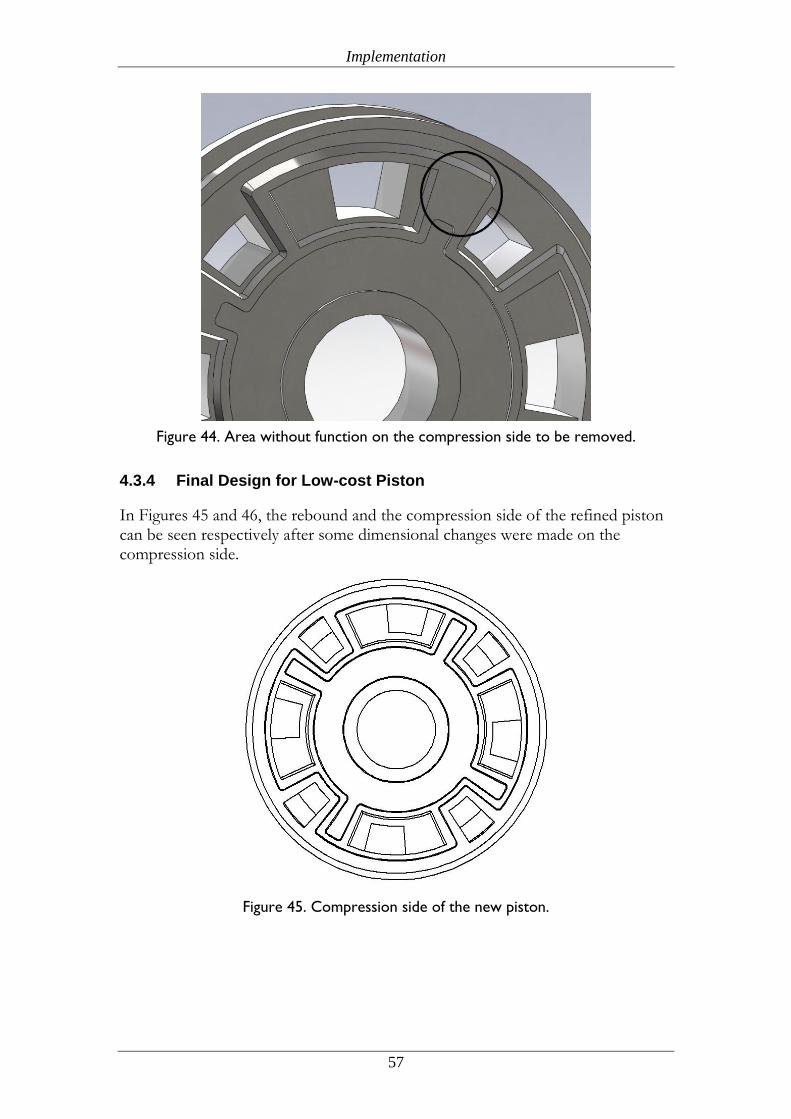
Implementation
57
Figure 44. Area without function on the compression side to be removed.
4.3.4 Final Design for Low-cost Piston
In Figures 45 and 46, the rebound and the compression side of the refined piston can be seen respectively after some dimensional changes were made on the compression side.
Figure 45. Compression side of the new piston.
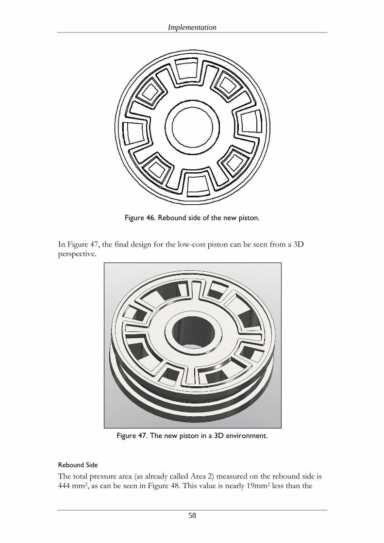
Implementation
58
Figure 46. Rebound side of the new piston.
In Figure 47, the final design for the low-cost piston can be seen from a 3D perspective.
Figure 47. The new piston in a 3D environment.
Rebound Side
The total pressure area (as already called Area 2) measured on the rebound side is 444 mm2, as can be seen in Figure 48. This value is nearly 19mm2 less than the
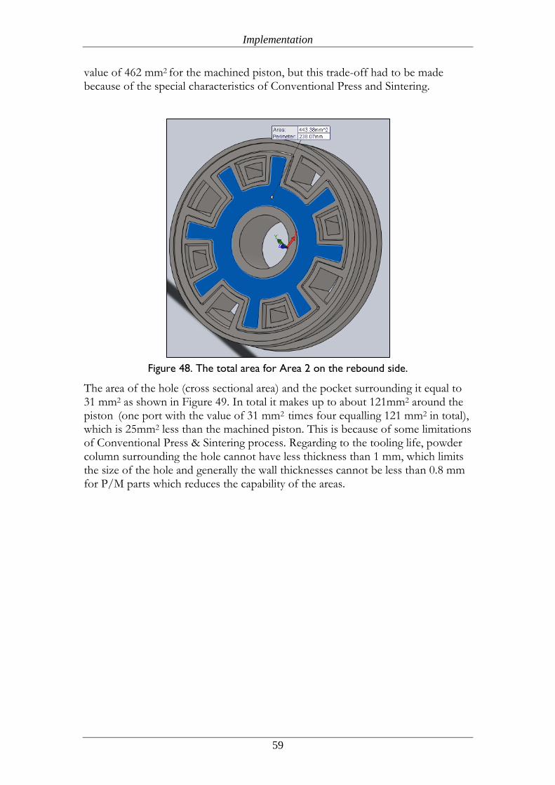
Implementation
59
value of 462 mm2 for the machined piston, but this trade-off had to be made because of the special characteristics of Conventional Press and Sintering.
Figure 48. The total area for Area 2 on the rebound side.
The area of the hole (cross sectional area) and the pocket surrounding it equal to 31 mm2 as shown in Figure 49. In total it makes up to about 121mm2 around the piston (one port with the value of 31 mm2 times four equalling 121 mm2 in total), which is 25mm2 less than the machined piston. This is because of some limitations of Conventional Press & Sintering process. Regarding to the tooling life, powder column surrounding the hole cannot have less thickness than 1 mm, which limits the size of the hole and generally the wall thicknesses cannot be less than 0.8 mm for P/M parts which reduces the capability of the areas.
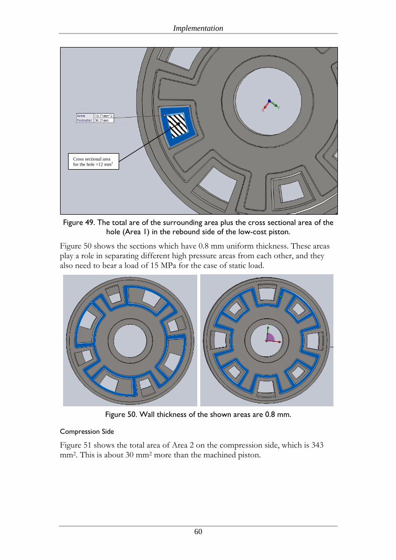
Implementation
60
Figure 49. The total are of the surrounding area plus the cross sectional area of the
hole (Area 1) in the rebound side of the low-cost piston.
Figure 50 shows the sections which have 0.8 mm uniform thickness. These areas play a role in separating different high pressure areas from each other, and they also need to bear a load of 15 MPa for the case of static load.
Figure 50. Wall thickness of the shown areas are 0.8 mm.
Compression Side
Figure 51 shows the total area of Area 2 on the compression side, which is 343 mm2. This is about 30 mm2 more than the machined piston.
Cross sectional area
for the hole =12 mm2
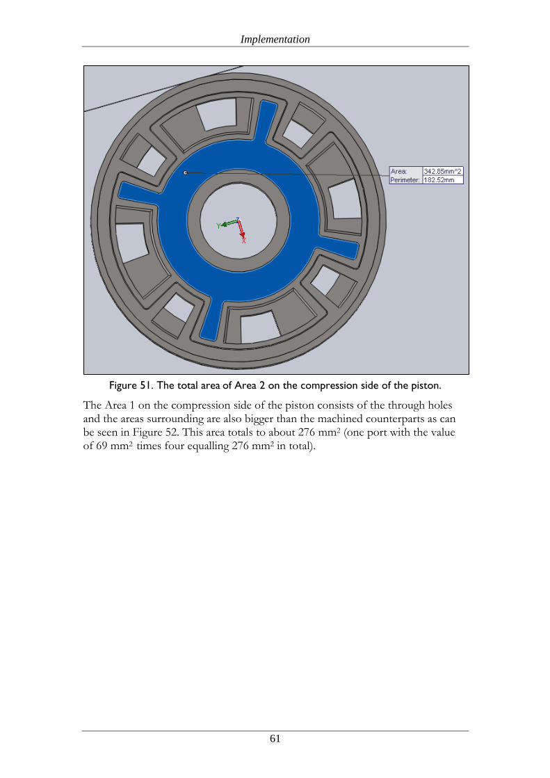
Implementation
61
Figure 51. The total area of Area 2 on the compression side of the piston.
The Area 1 on the compression side of the piston consists of the through holes and the areas surrounding are also bigger than the machined counterparts as can be seen in Figure 52. This area totals to about 276 mm2 (one port with the value of 69 mm2 times four equalling 276 mm2 in total).
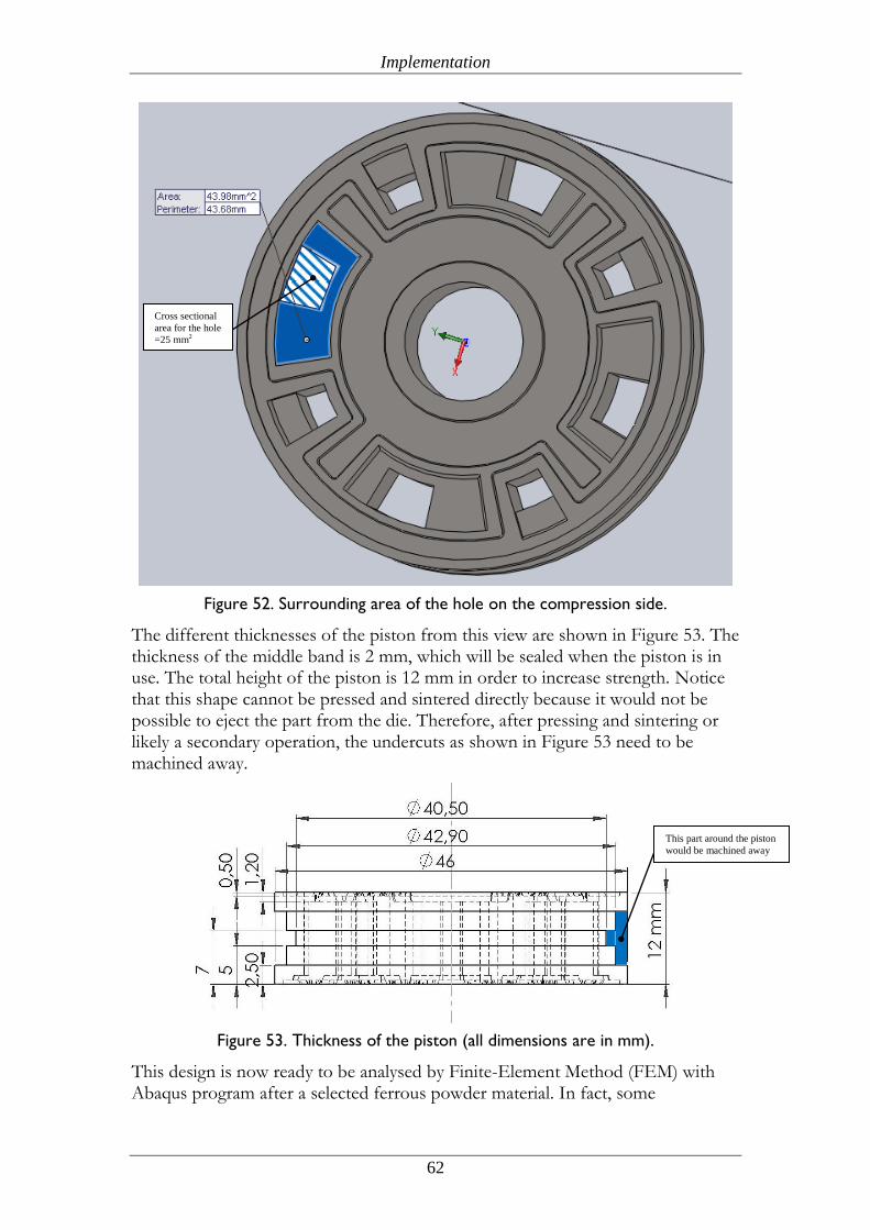
Implementation
62
Figure 52. Surrounding area of the hole on the compression side.
The different thicknesses of the piston from this view are shown in Figure 53. The thickness of the middle band is 2 mm, which will be sealed when the piston is in use. The total height of the piston is 12 mm in order to increase strength. Notice that this shape cannot be pressed and sintered directly because it would not be possible to eject the part from the die. Therefore, after pressing and sintering or likely a secondary operation, the undercuts as shown in Figure 53 need to be machined away.
Figure 53. Thickness of the piston (all dimensions are in mm).
This design is now ready to be analysed by Finite-Element Method (FEM) with Abaqus program after a selected ferrous powder material. In fact, some
Cross sectional
area for the hole
=25 mm2
This part around the piston
would be machined away
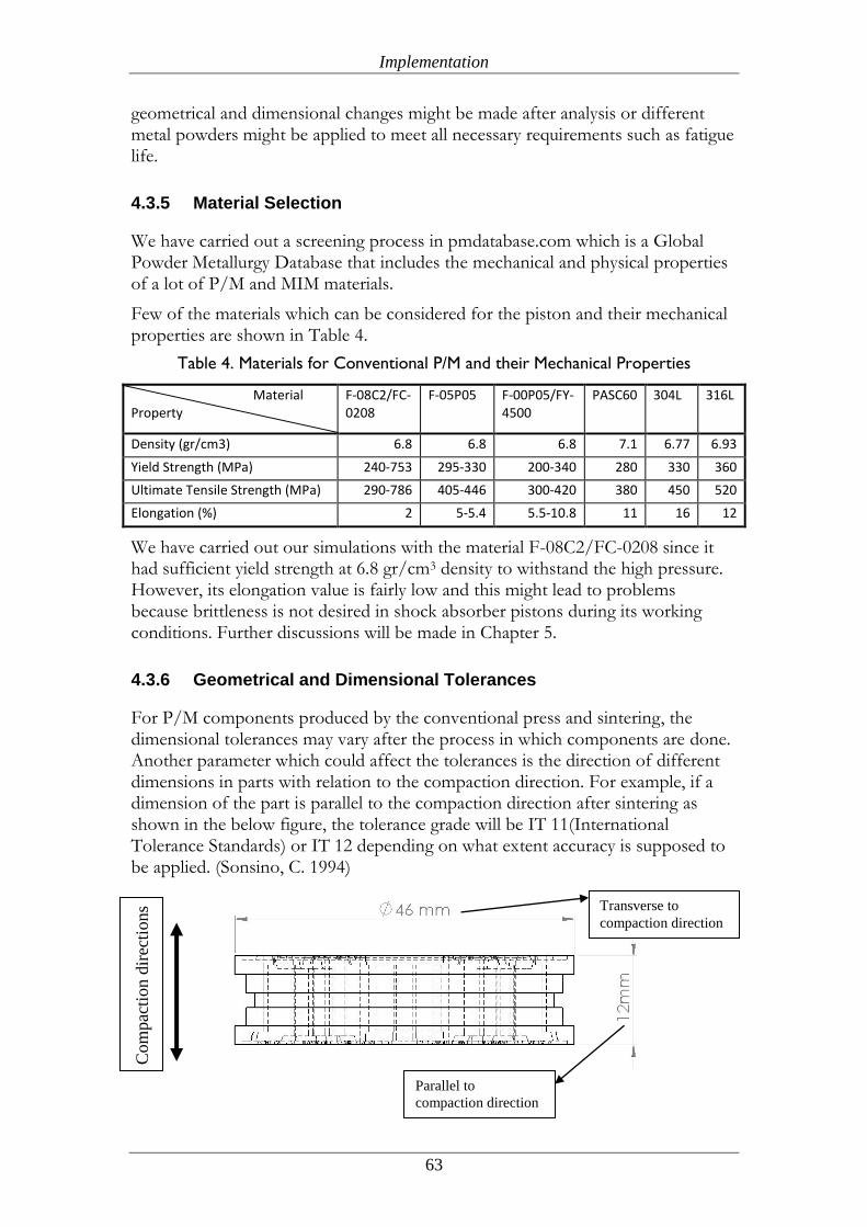
Implementation
63
geometrical and dimensional changes might be made after analysis or different metal powders might be applied to meet all necessary requirements such as fatigue life.
4.3.5 Material Selection
We have carried out a screening process in pmdatabase.com which is a Global Powder Metallurgy Database that includes the mechanical and physical properties of a lot of P/M and MIM materials.
Few of the materials which can be considered for the piston and their mechanical properties are shown in Table 4.
Table 4. Materials for Conventional P/M and their Mechanical Properties
Material Property
F-08C2/FC-0208
F-05P05 F-00P05/FY-4500
PASC60 304L 316L
Density (gr/cm3) 6.8 6.8 6.8 7.1 6.77 6.93
Yield Strength (MPa) 240-753 295-330 200-340 280 330 360
Ultimate Tensile Strength (MPa) 290-786 405-446 300-420 380 450 520
Elongation (%) 2 5-5.4 5.5-10.8 11 16 12
We have carried out our simulations with the material F-08C2/FC-0208 since it had sufficient yield strength at 6.8 gr/cm3 density to withstand the high pressure. However, its elongation value is fairly low and this might lead to problems because brittleness is not desired in shock absorber pistons during its working conditions. Further discussions will be made in Chapter 5.
4.3.6 Geometrical and Dimensional Tolerances
For P/M components produced by the conventional press and sintering, the dimensional tolerances may vary after the process in which components are done. Another parameter which could affect the tolerances is the direction of different dimensions in parts with relation to the compaction direction. For example, if a dimension of the part is parallel to the compaction direction after sintering as shown in the below figure, the tolerance grade will be IT 11(International Tolerance Standards) or IT 12 depending on what extent accuracy is supposed to be applied. (Sonsino, C. 1994)
Com
pac
tion d
irec
tions Transverse to
compaction direction
Parallel to
compaction direction
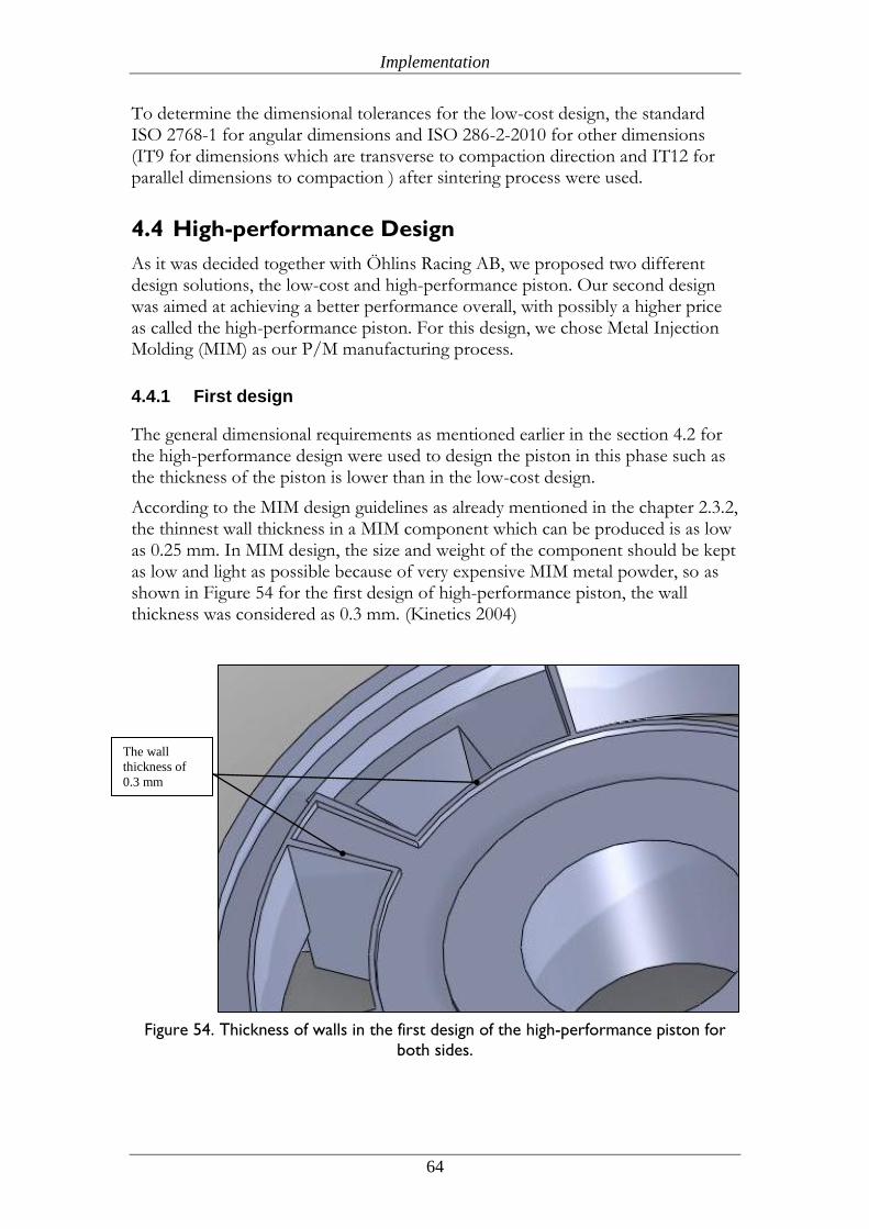
Implementation
64
To determine the dimensional tolerances for the low-cost design, the standard ISO 2768-1 for angular dimensions and ISO 286-2-2010 for other dimensions (IT9 for dimensions which are transverse to compaction direction and IT12 for parallel dimensions to compaction ) after sintering process were used.
4.4 High-performance Design
As it was decided together with Öhlins Racing AB, we proposed two different design solutions, the low-cost and high-performance piston. Our second design was aimed at achieving a better performance overall, with possibly a higher price as called the high-performance piston. For this design, we chose Metal Injection Molding (MIM) as our P/M manufacturing process.
4.4.1 First design
The general dimensional requirements as mentioned earlier in the section 4.2 for the high-performance design were used to design the piston in this phase such as the thickness of the piston is lower than in the low-cost design.
According to the MIM design guidelines as already mentioned in the chapter 2.3.2, the thinnest wall thickness in a MIM component which can be produced is as low as 0.25 mm. In MIM design, the size and weight of the component should be kept as low and light as possible because of very expensive MIM metal powder, so as shown in Figure 54 for the first design of high-performance piston, the wall thickness was considered as 0.3 mm. (Kinetics 2004)
Figure 54. Thickness of walls in the first design of the high-performance piston for
both sides.
The wall
thickness of
0.3 mm
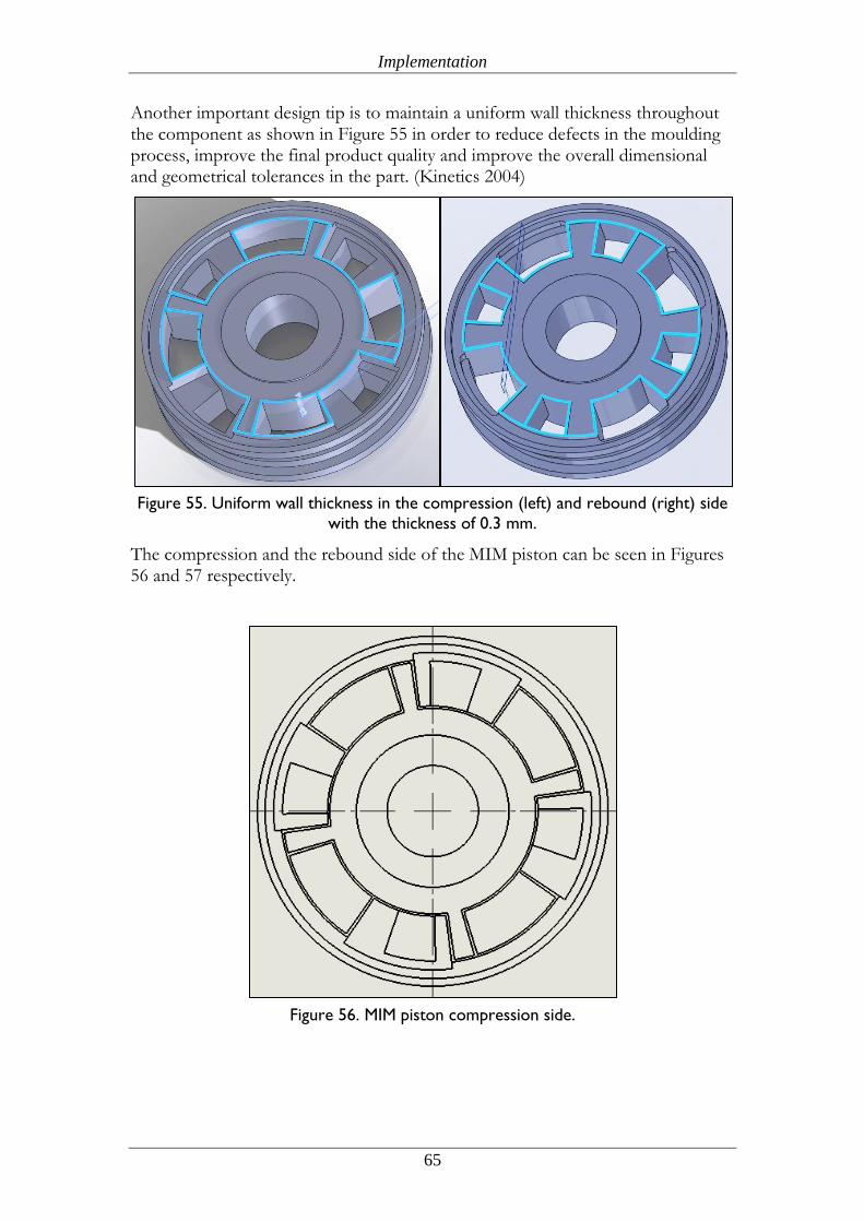
Implementation
65
Another important design tip is to maintain a uniform wall thickness throughout the component as shown in Figure 55 in order to reduce defects in the moulding process, improve the final product quality and improve the overall dimensional and geometrical tolerances in the part. (Kinetics 2004)
Figure 55. Uniform wall thickness in the compression (left) and rebound (right) side
with the thickness of 0.3 mm.
The compression and the rebound side of the MIM piston can be seen in Figures 56 and 57 respectively.
Figure 56. MIM piston compression side.
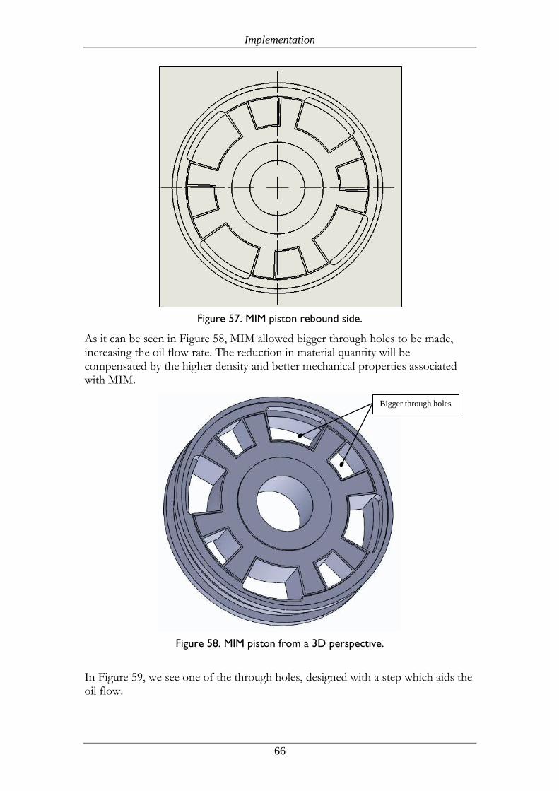
Implementation
66
Figure 57. MIM piston rebound side.
As it can be seen in Figure 58, MIM allowed bigger through holes to be made, increasing the oil flow rate. The reduction in material quantity will be compensated by the higher density and better mechanical properties associated with MIM.
Figure 58. MIM piston from a 3D perspective.
In Figure 59, we see one of the through holes, designed with a step which aids the oil flow.
Bigger through holes
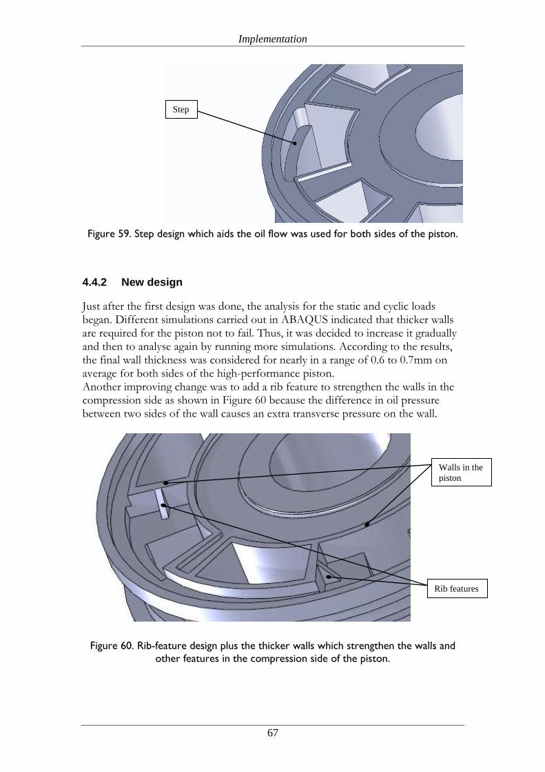
Implementation
67
Figure 59. Step design which aids the oil flow was used for both sides of the piston.
4.4.2 New design
Just after the first design was done, the analysis for the static and cyclic loads began. Different simulations carried out in ABAQUS indicated that thicker walls are required for the piston not to fail. Thus, it was decided to increase it gradually and then to analyse again by running more simulations. According to the results, the final wall thickness was considered for nearly in a range of 0.6 to 0.7mm on average for both sides of the high-performance piston. Another improving change was to add a rib feature to strengthen the walls in the compression side as shown in Figure 60 because the difference in oil pressure between two sides of the wall causes an extra transverse pressure on the wall.
Figure 60. Rib-feature design plus the thicker walls which strengthen the walls and
other features in the compression side of the piston.
Step
Rib features
Walls in the
piston
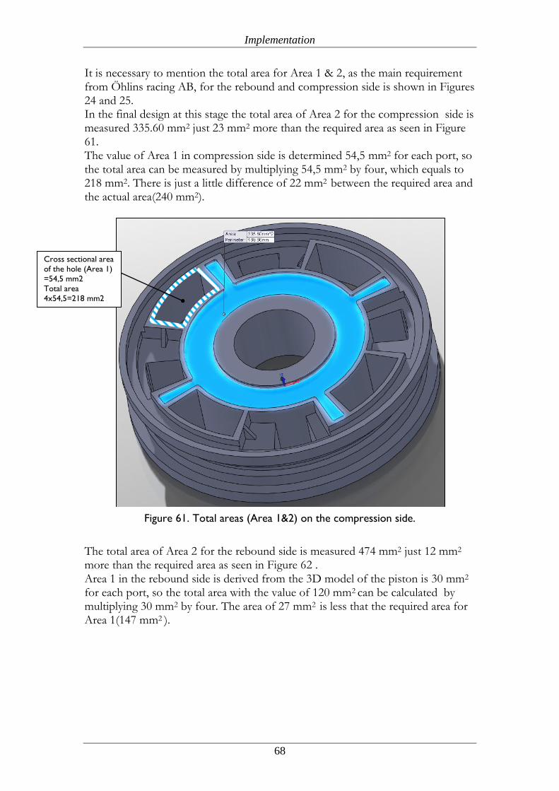
Implementation
68
It is necessary to mention the total area for Area 1 & 2, as the main requirement from Öhlins racing AB, for the rebound and compression side is shown in Figures 24 and 25. In the final design at this stage the total area of Area 2 for the compression side is measured 335.60 mm2 just 23 mm2 more than the required area as seen in Figure 61. The value of Area 1 in compression side is determined 54,5 mm2 for each port, so the total area can be measured by multiplying 54,5 mm2 by four, which equals to 218 mm2. There is just a little difference of 22 mm2 between the required area and the actual area(240 mm2).
Figure 61. Total areas (Area 1&2) on the compression side.
The total area of Area 2 for the rebound side is measured 474 mm2 just 12 mm2 more than the required area as seen in Figure 62 . Area 1 in the rebound side is derived from the 3D model of the piston is 30 mm2 for each port, so the total area with the value of 120 mm2 can be calculated by multiplying 30 mm2 by four. The area of 27 mm2 is less that the required area for Area 1(147 mm2 ).
Cross sectional area
of the hole (Area 1)
=54,5 mm2
Total area
4x54,5=218 mm2
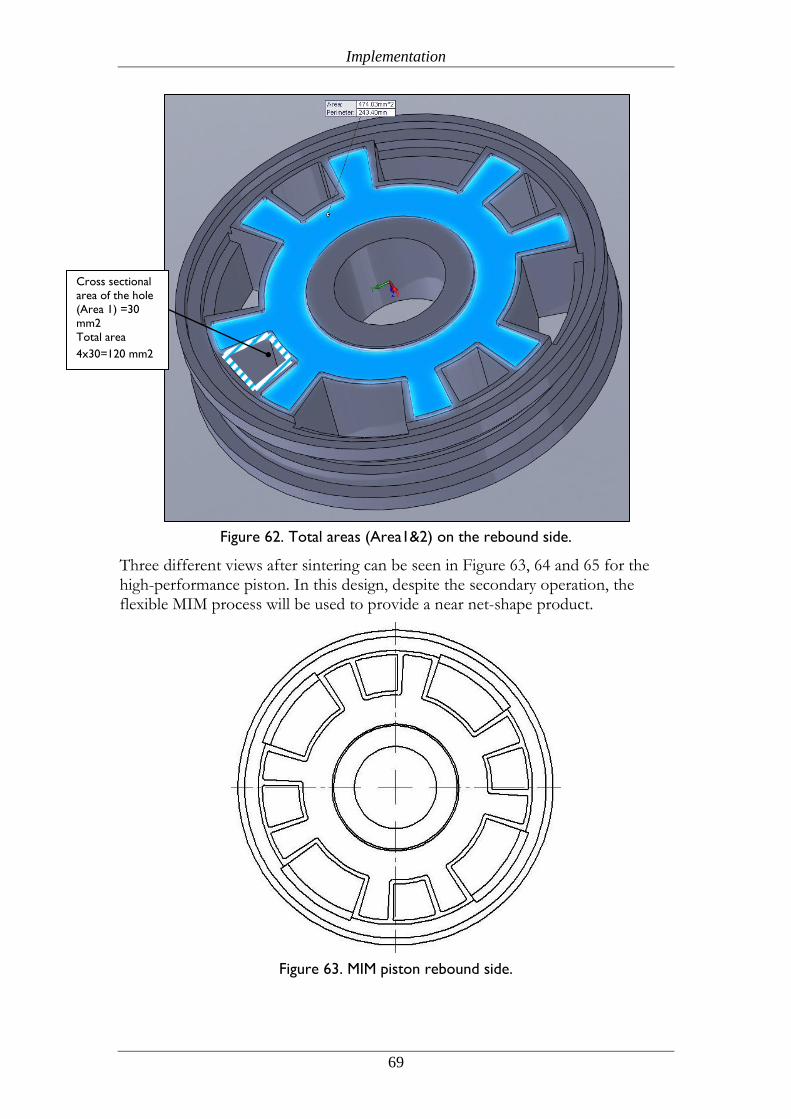
Implementation
69
Figure 62. Total areas (Area1&2) on the rebound side.
Three different views after sintering can be seen in Figure 63, 64 and 65 for the high-performance piston. In this design, despite the secondary operation, the flexible MIM process will be used to provide a near net-shape product.
Figure 63. MIM piston rebound side.
Cross sectional
area of the hole
(Area 1) =30
mm2
Total area
4x30=120 mm2
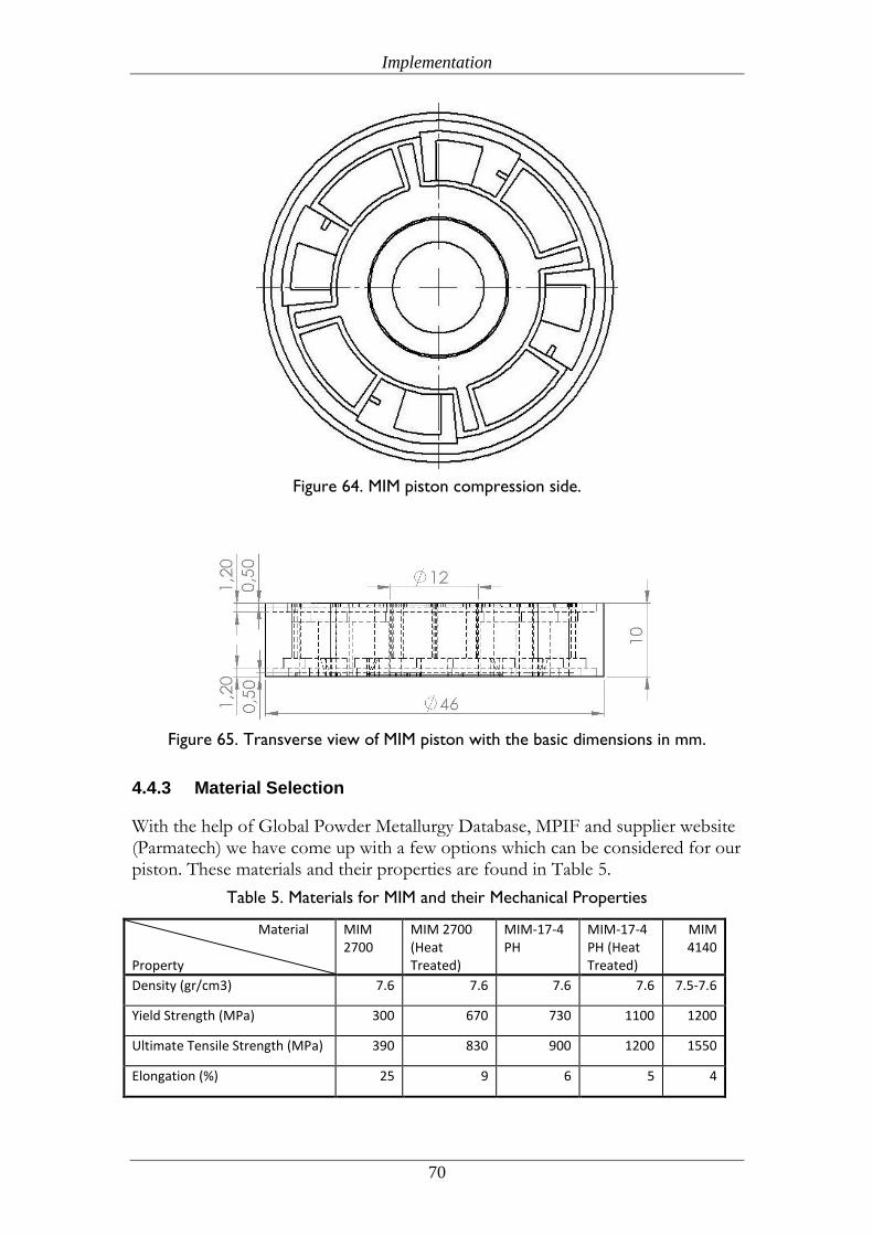
Implementation
70
Figure 64. MIM piston compression side.
Figure 65. Transverse view of MIM piston with the basic dimensions in mm.
4.4.3 Material Selection
With the help of Global Powder Metallurgy Database, MPIF and supplier website (Parmatech) we have come up with a few options which can be considered for our piston. These materials and their properties are found in Table 5.
Table 5. Materials for MIM and their Mechanical Properties
Material
Property
MIM 2700
MIM 2700 (Heat Treated)
MIM-17-4 PH
MIM-17-4 PH (Heat Treated)
MIM 4140
Density (gr/cm3) 7.6 7.6 7.6 7.6 7.5-7.6
Yield Strength (MPa) 300 670 730 1100 1200
Ultimate Tensile Strength (MPa) 390 830 900 1200 1550
Elongation (%) 25 9 6 5 4
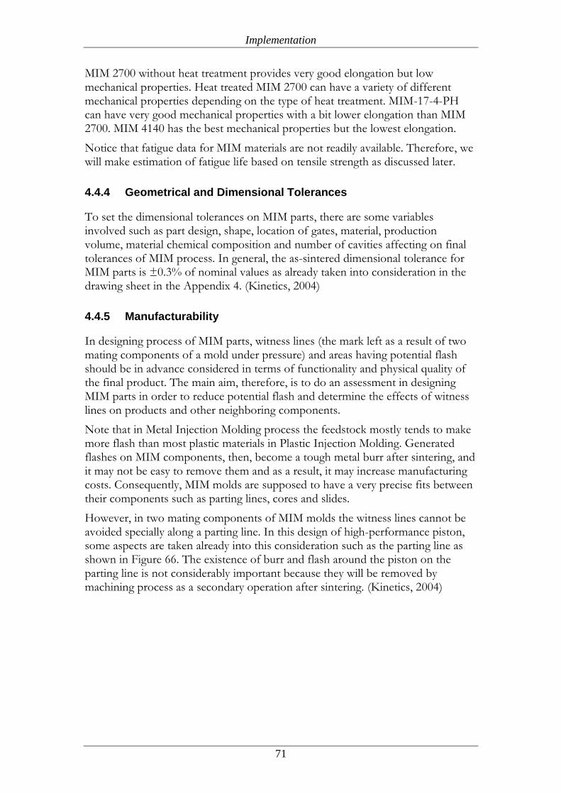
Implementation
71
MIM 2700 without heat treatment provides very good elongation but low mechanical properties. Heat treated MIM 2700 can have a variety of different mechanical properties depending on the type of heat treatment. MIM-17-4-PH can have very good mechanical properties with a bit lower elongation than MIM 2700. MIM 4140 has the best mechanical properties but the lowest elongation.
Notice that fatigue data for MIM materials are not readily available. Therefore, we will make estimation of fatigue life based on tensile strength as discussed later.
4.4.4 Geometrical and Dimensional Tolerances
To set the dimensional tolerances on MIM parts, there are some variables involved such as part design, shape, location of gates, material, production volume, material chemical composition and number of cavities affecting on final tolerances of MIM process. In general, the as-sintered dimensional tolerance for MIM parts is ±0.3% of nominal values as already taken into consideration in the drawing sheet in the Appendix 4. (Kinetics, 2004)
4.4.5 Manufacturability
In designing process of MIM parts, witness lines (the mark left as a result of two mating components of a mold under pressure) and areas having potential flash should be in advance considered in terms of functionality and physical quality of the final product. The main aim, therefore, is to do an assessment in designing MIM parts in order to reduce potential flash and determine the effects of witness lines on products and other neighboring components.
Note that in Metal Injection Molding process the feedstock mostly tends to make more flash than most plastic materials in Plastic Injection Molding. Generated flashes on MIM components, then, become a tough metal burr after sintering, and it may not be easy to remove them and as a result, it may increase manufacturing costs. Consequently, MIM molds are supposed to have a very precise fits between their components such as parting lines, cores and slides.
However, in two mating components of MIM molds the witness lines cannot be avoided specially along a parting line. In this design of high-performance piston, some aspects are taken already into this consideration such as the parting line as shown in Figure 66. The existence of burr and flash around the piston on the parting line is not considerably important because they will be removed by machining process as a secondary operation after sintering. (Kinetics, 2004)
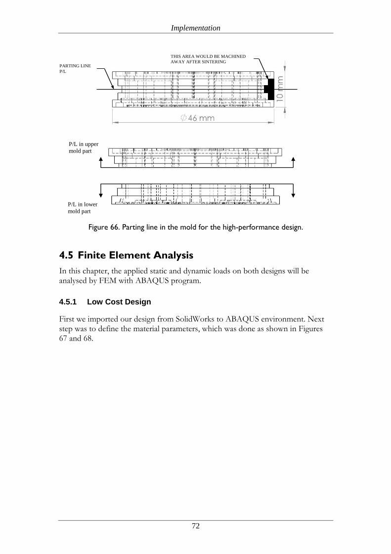
Implementation
72
Figure 66. Parting line in the mold for the high-performance design.
4.5 Finite Element Analysis
In this chapter, the applied static and dynamic loads on both designs will be analysed by FEM with ABAQUS program.
4.5.1 Low Cost Design
First we imported our design from SolidWorks to ABAQUS environment. Next step was to define the material parameters, which was done as shown in Figures 67 and 68.
PARTING LINE
P/L
THIS AREA WOULD BE MACHINED
AWAY AFTER SINTERING
P/L in upper
mold part
P/L in lower
mold part
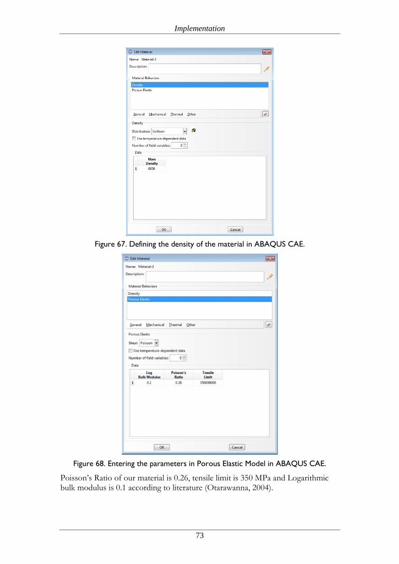
Implementation
73
Figure 67. Defining the density of the material in ABAQUS CAE.
Figure 68. Entering the parameters in Porous Elastic Model in ABAQUS CAE.
Poisson’s Ratio of our material is 0.26, tensile limit is 350 MPa and Logarithmic bulk modulus is 0.1 according to literature (Otarawanna, 2004).
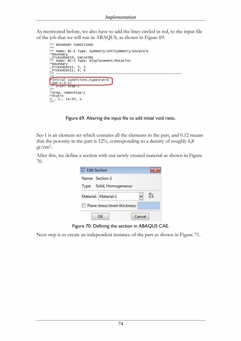
Implementation
74
As mentioned before, we also have to add the lines circled in red, to the input file of the job that we will run in ABAQUS, as shown in Figure 69.
Figure 69. Altering the input file to add initial void ratio.
Set-1 is an element set which contains all the elements in the part, and 0.12 means that the porosity in the part is 12%, corresponding to a density of roughly 6,8 gr/cm3.
After this, we define a section with our newly created material as shown in Figure 70.
Figure 70. Defining the section in ABAQUS CAE.
Next step is to create an independent instance of the part as shown in Figure 71.
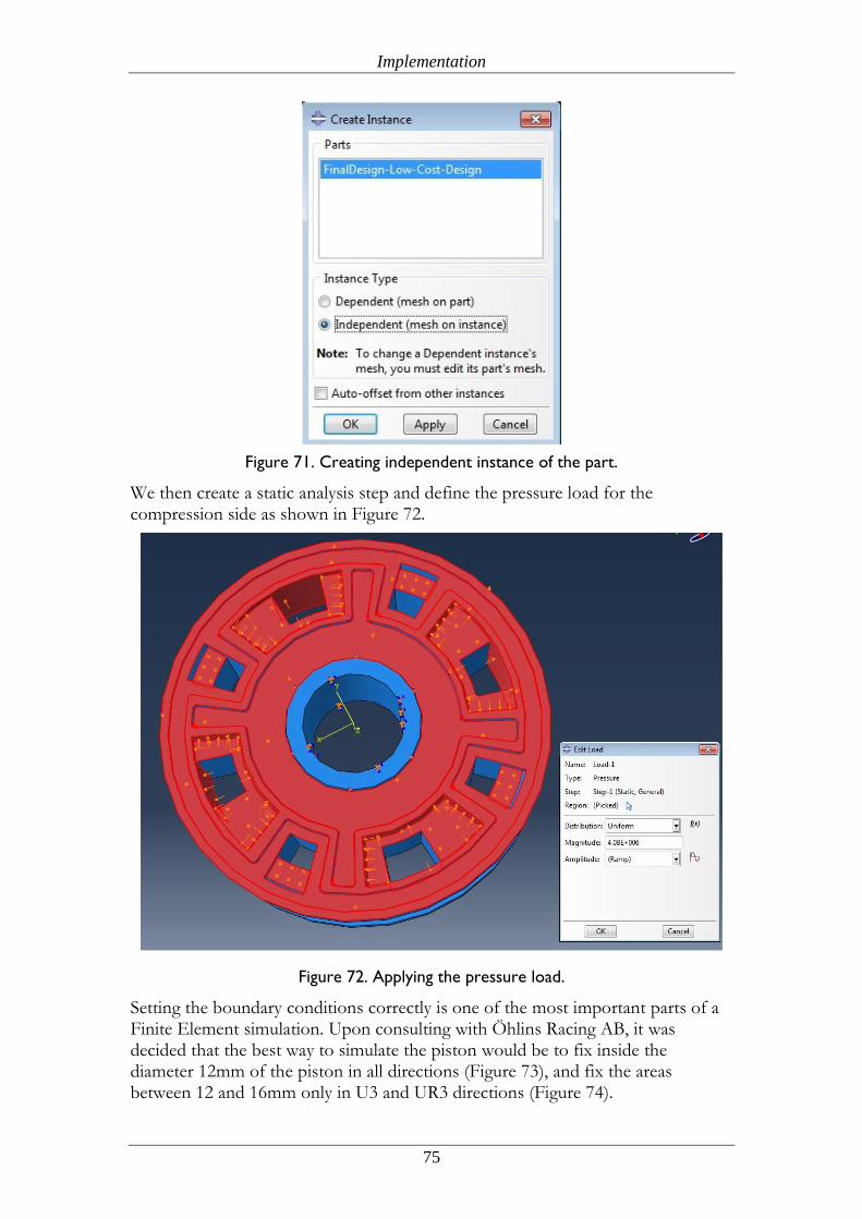
Implementation
75
Figure 71. Creating independent instance of the part.
We then create a static analysis step and define the pressure load for the compression side as shown in Figure 72.
Figure 72. Applying the pressure load.
Setting the boundary conditions correctly is one of the most important parts of a Finite Element simulation. Upon consulting with Öhlins Racing AB, it was decided that the best way to simulate the piston would be to fix inside the diameter 12mm of the piston in all directions (Figure 73), and fix the areas between 12 and 16mm only in U3 and UR3 directions (Figure 74).
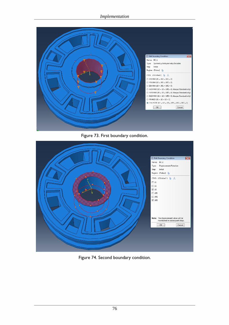
Implementation
76
Figure 73. First boundary condition.
Figure 74. Second boundary condition.
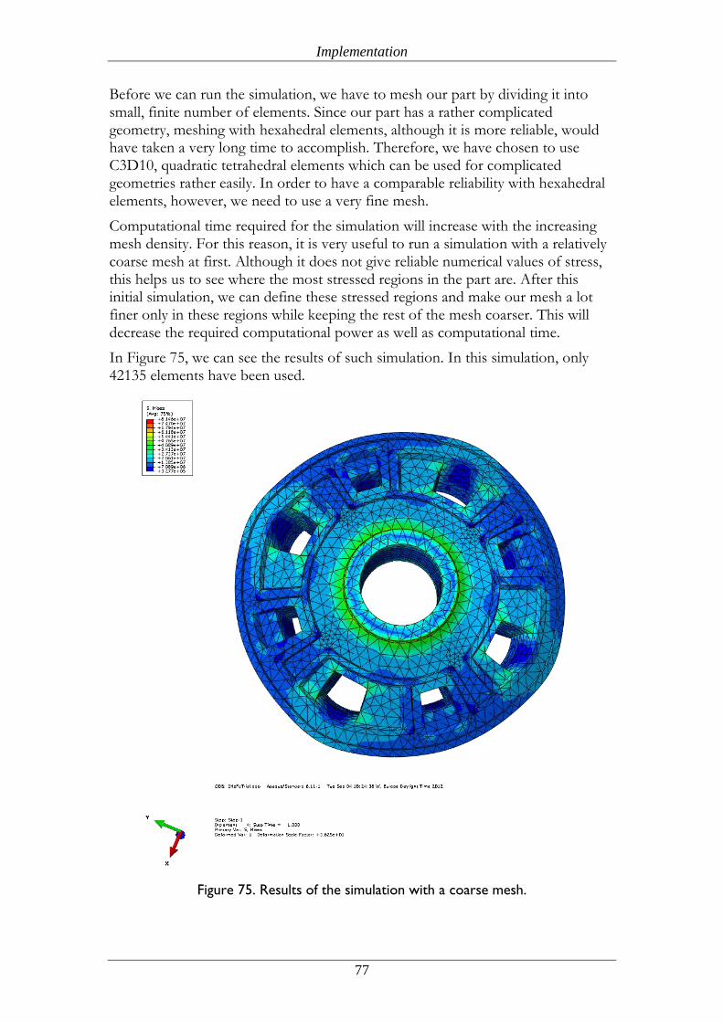
Implementation
77
Before we can run the simulation, we have to mesh our part by dividing it into small, finite number of elements. Since our part has a rather complicated geometry, meshing with hexahedral elements, although it is more reliable, would have taken a very long time to accomplish. Therefore, we have chosen to use C3D10, quadratic tetrahedral elements which can be used for complicated geometries rather easily. In order to have a comparable reliability with hexahedral elements, however, we need to use a very fine mesh.
Computational time required for the simulation will increase with the increasing mesh density. For this reason, it is very useful to run a simulation with a relatively coarse mesh at first. Although it does not give reliable numerical values of stress, this helps us to see where the most stressed regions in the part are. After this initial simulation, we can define these stressed regions and make our mesh a lot finer only in these regions while keeping the rest of the mesh coarser. This will decrease the required computational power as well as computational time.
In Figure 75, we can see the results of such simulation. In this simulation, only 42135 elements have been used.
Figure 75. Results of the simulation with a coarse mesh.
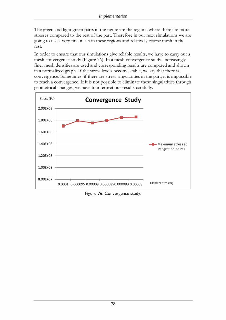
Implementation
78
The green and light green parts in the figure are the regions where there are more stresses compared to the rest of the part. Therefore in our next simulations we are going to use a very fine mesh in these regions and relatively coarse mesh in the rest.
In order to ensure that our simulations give reliable results, we have to carry out a mesh convergence study (Figure 76). In a mesh convergence study, increasingly finer mesh densities are used and corresponding results are compared and shown in a normalized graph. If the stress levels become stable, we say that there is convergence. Sometimes, if there are stress singularities in the part, it is impossible to reach a convergence. If it is not possible to eliminate these singularities through geometrical changes, we have to interpret our results carefully.
Figure 76. Convergence study.
8.00E+07
1.00E+08
1.20E+08
1.40E+08
1.60E+08
1.80E+08
2.00E+08
0.0001 0.000095 0.00009 0.0000850.000083 0.00008
Convergence Study
Maximum stress atintegration points
Stress (Pa)
Element size (m)
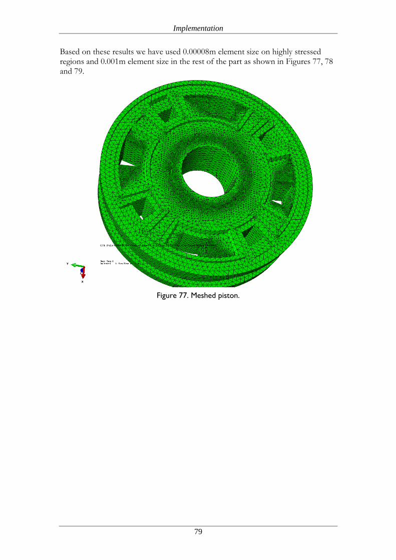
Implementation
79
Based on these results we have used 0.00008m element size on highly stressed regions and 0.001m element size in the rest of the part as shown in Figures 77, 78 and 79.
Figure 77. Meshed piston.
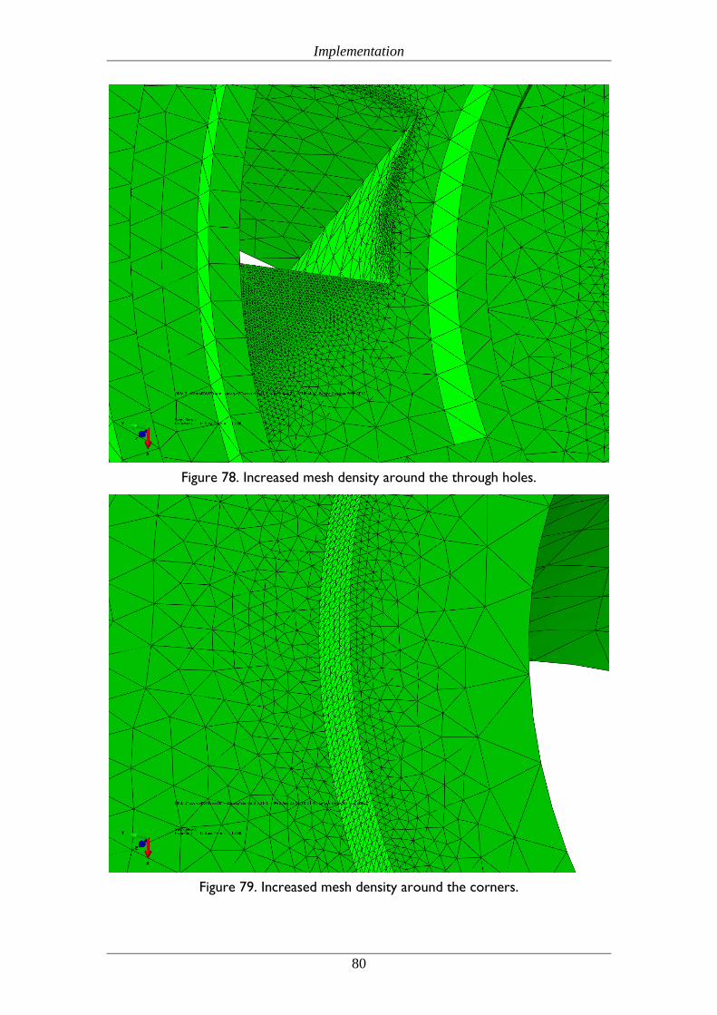
Implementation
80
Figure 78. Increased mesh density around the through holes.
Figure 79. Increased mesh density around the corners.
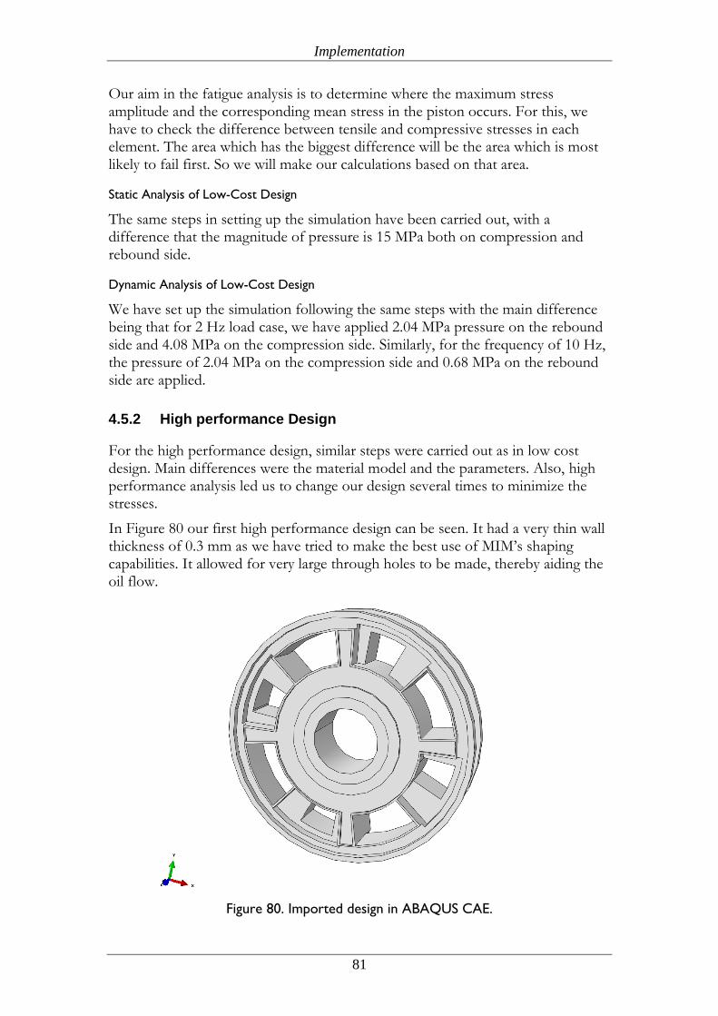
Implementation
81
Our aim in the fatigue analysis is to determine where the maximum stress amplitude and the corresponding mean stress in the piston occurs. For this, we have to check the difference between tensile and compressive stresses in each element. The area which has the biggest difference will be the area which is most likely to fail first. So we will make our calculations based on that area.
Static Analysis of Low-Cost Design
The same steps in setting up the simulation have been carried out, with a difference that the magnitude of pressure is 15 MPa both on compression and rebound side.
Dynamic Analysis of Low-Cost Design
We have set up the simulation following the same steps with the main difference being that for 2 Hz load case, we have applied 2.04 MPa pressure on the rebound side and 4.08 MPa on the compression side. Similarly, for the frequency of 10 Hz, the pressure of 2.04 MPa on the compression side and 0.68 MPa on the rebound side are applied.
4.5.2 High performance Design
For the high performance design, similar steps were carried out as in low cost design. Main differences were the material model and the parameters. Also, high performance analysis led us to change our design several times to minimize the stresses.
In Figure 80 our first high performance design can be seen. It had a very thin wall thickness of 0.3 mm as we have tried to make the best use of MIM’s shaping capabilities. It allowed for very large through holes to be made, thereby aiding the oil flow.
Figure 80. Imported design in ABAQUS CAE.
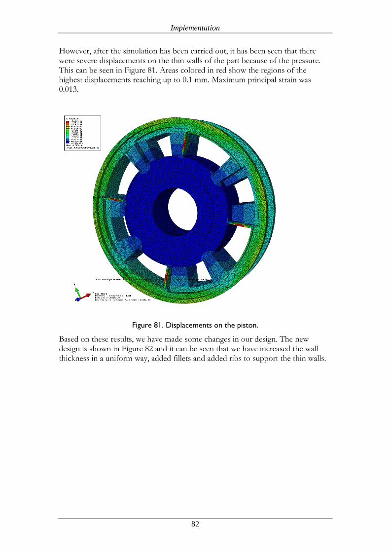
Implementation
82
However, after the simulation has been carried out, it has been seen that there were severe displacements on the thin walls of the part because of the pressure. This can be seen in Figure 81. Areas colored in red show the regions of the highest displacements reaching up to 0.1 mm. Maximum principal strain was 0.013.
Figure 81. Displacements on the piston.
Based on these results, we have made some changes in our design. The new design is shown in Figure 82 and it can be seen that we have increased the wall thickness in a uniform way, added fillets and added ribs to support the thin walls.
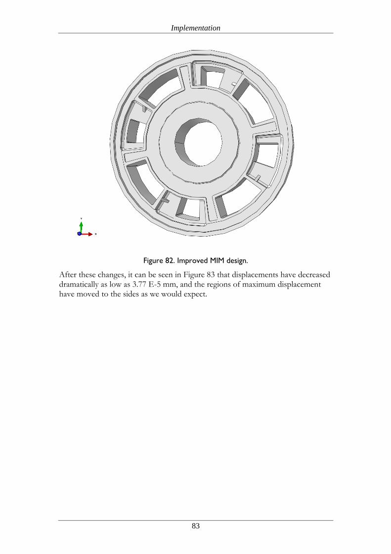
Implementation
83
Figure 82. Improved MIM design.
After these changes, it can be seen in Figure 83 that displacements have decreased dramatically as low as 3.77 E-5 mm, and the regions of maximum displacement have moved to the sides as we would expect.
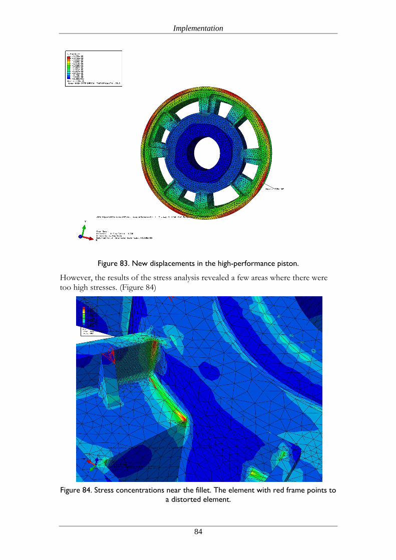
Implementation
84
Figure 83. New displacements in the high-performance piston.
However, the results of the stress analysis revealed a few areas where there were too high stresses. (Figure 84)
Figure 84. Stress concentrations near the fillet. The element with red frame points to
a distorted element.
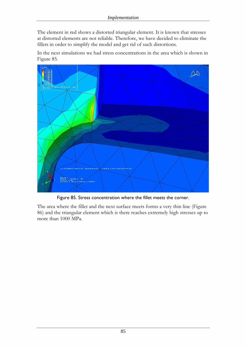
Implementation
85
The element in red shows a distorted triangular element. It is known that stresses at distorted elements are not reliable. Therefore, we have decided to eliminate the fillets in order to simplify the model and get rid of such distortions.
In the next simulations we had stress concentrations in the area which is shown in Figure 85.
Figure 85. Stress concentration where the fillet meets the corner.
The area where the fillet and the next surface meets forms a very thin line (Figure 86) and the triangular element which is there reaches extremely high stresses up to more than 1000 MPa.
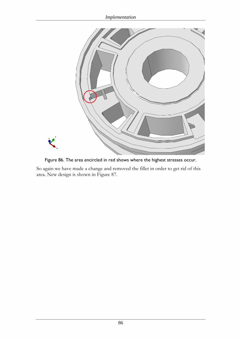
Implementation
86
Figure 86. The area encircled in red shows where the highest stresses occur.
So again we have made a change and removed the fillet in order to get rid of this area. New design is shown in Figure 87.
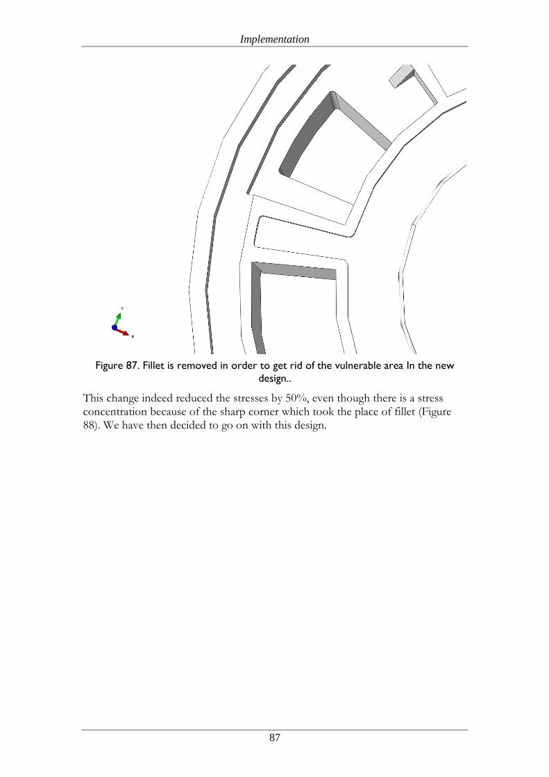
Implementation
87
Figure 87. Fillet is removed in order to get rid of the vulnerable area In the new
design..
This change indeed reduced the stresses by 50%, even though there is a stress concentration because of the sharp corner which took the place of fillet (Figure 88). We have then decided to go on with this design.
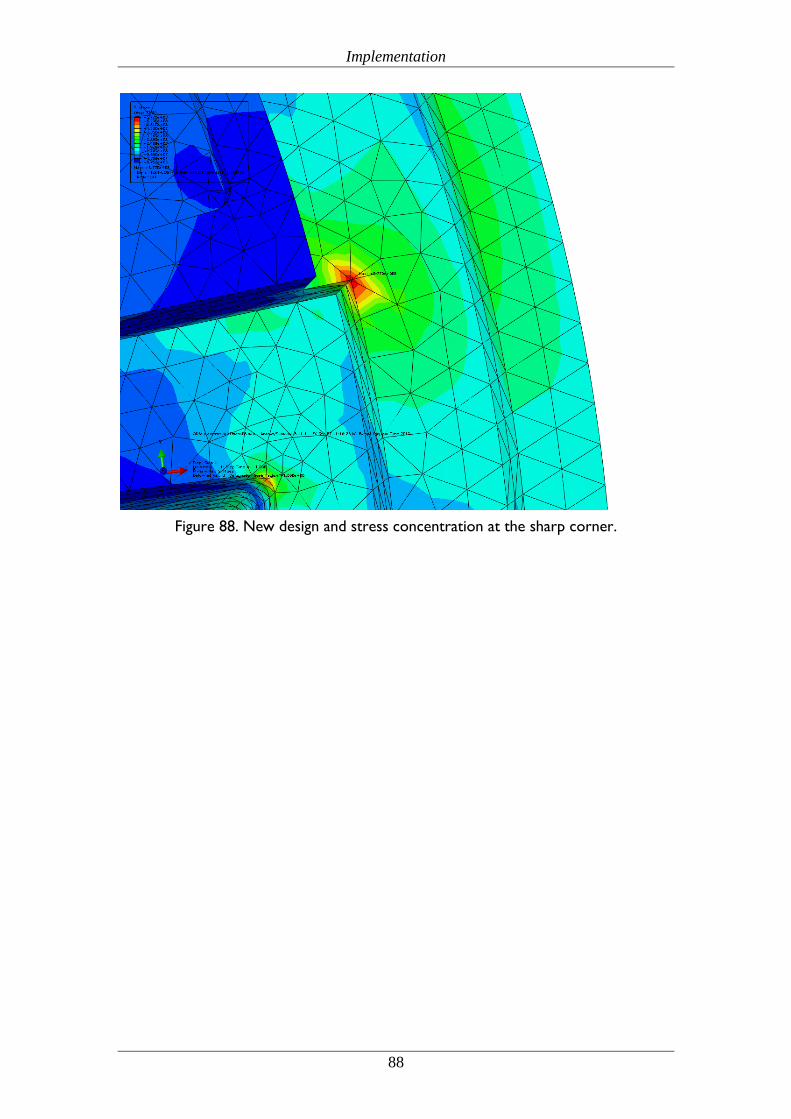
Implementation
88
Figure 88. New design and stress concentration at the sharp corner.
Findings and Analysis
89
5 Findings and Analysis
5.1 Stress Analysis
According to the product development method already mentioned in the chapter 3, the stress analysis is carried out for the high-performance and the low-cost designs. The main aim of this analysis will be to find out the maximum local stress and maximum allowable local stress of the piston in terms of the static and cyclic loading modes for each design in this part.
5.1.1 Low-Cost Piston
For the low-cost piston, we got the results of static loading and dynamic loading separately.
Static Loading
Because of the complicated geometry and constrained regions, there occurred some stress singularities in the piston. As a result of the simulation, the highest stress seemed to be around 450 MPa for the compression side and 348 MPa for the rebound side. This is indeed higher than the yield strength of our material, but when we analyze the part overall, we can see that only a number of elements have higher stresses than 250 MPa and these elements are at the intersection between a constrained and unconstrained region and at areas where the stress goes to infinity in a single element. It is obvious that these do not represent real conditions, so we can say that the highest stresses in the part are below the yield strength of our material.
Cyclic Loading (Fatigue Analysis)
The maximum tensile stresses ( ), maximum compressive stresses ( ) and
corresponding stress amplitudes ( ) can be seen in Appendix 5.
Here we have to take stress singularities into consideration. If we look at where the highest stresses are, we can see that these stresses are increased by stress singularities, and they do not represent a logical stress distribution. In a single element, there are huge differences between different nodes. Sometimes at node connection points (especially between constrained and unconstrained elements) and in regions where we apply a pressure on areas which are narrowing down and meeting at a point (since stress is force divided by area, if area becomes 0, stresses go to infinity), stresses may rise dramatically. Therefore, we have to make a logical assumption and ignore these highly stressed single nodes and continue our calculations with the next highly stressed region.
For the rebound side, highest stresses can be found in Appendix 6.
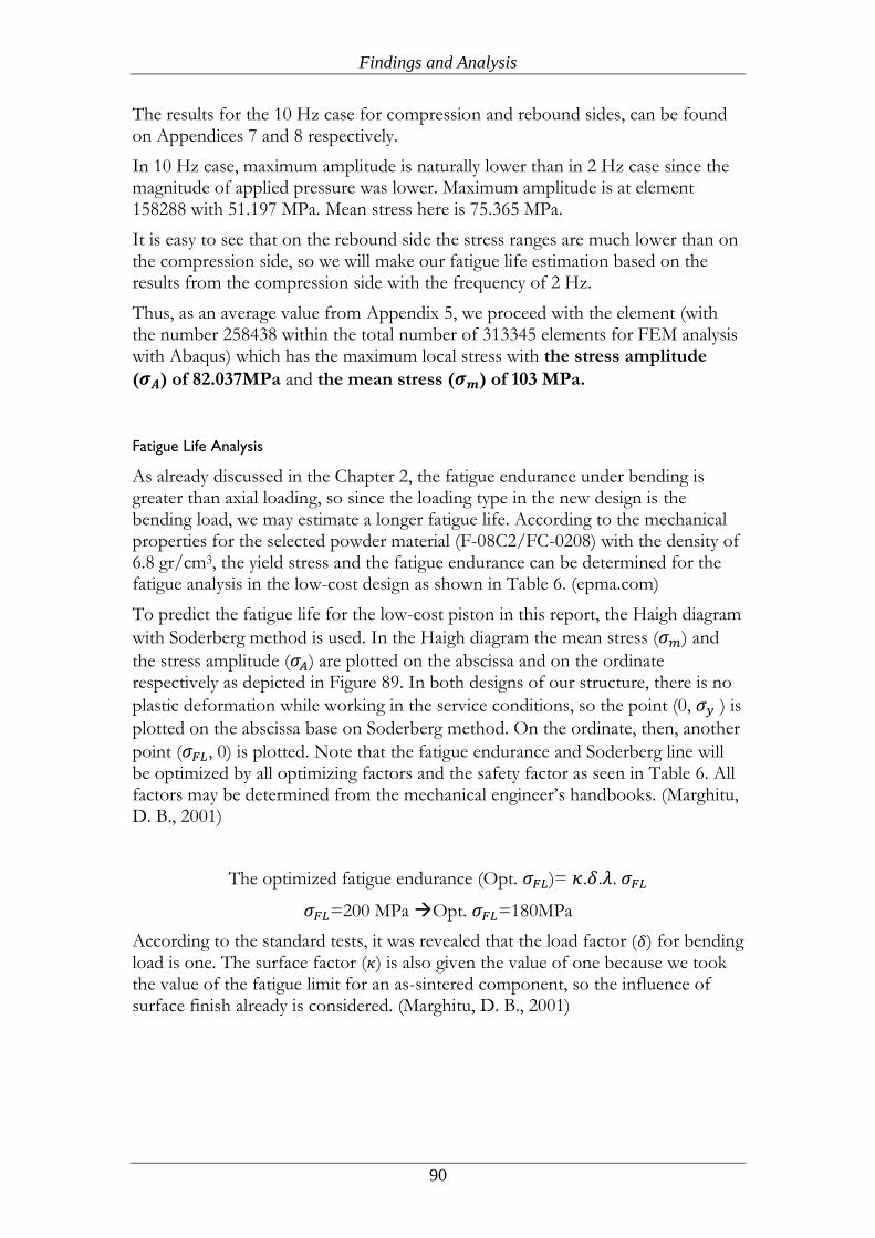
Findings and Analysis
90
The results for the 10 Hz case for compression and rebound sides, can be found on Appendices 7 and 8 respectively.
In 10 Hz case, maximum amplitude is naturally lower than in 2 Hz case since the magnitude of applied pressure was lower. Maximum amplitude is at element 158288 with 51.197 MPa. Mean stress here is 75.365 MPa.
It is easy to see that on the rebound side the stress ranges are much lower than on the compression side, so we will make our fatigue life estimation based on the results from the compression side with the frequency of 2 Hz.
Thus, as an average value from Appendix 5, we proceed with the element (with the number 258438 within the total number of 313345 elements for FEM analysis with Abaqus) which has the maximum local stress with the stress amplitude
( ) of 82.037MPa and the mean stress ( ) of 103 MPa.
Fatigue Life Analysis
As already discussed in the Chapter 2, the fatigue endurance under bending is greater than axial loading, so since the loading type in the new design is the bending load, we may estimate a longer fatigue life. According to the mechanical properties for the selected powder material (F-08C2/FC-0208) with the density of 6.8 gr/cm3, the yield stress and the fatigue endurance can be determined for the fatigue analysis in the low-cost design as shown in Table 6. (epma.com)
To predict the fatigue life for the low-cost piston in this report, the Haigh diagram
with Soderberg method is used. In the Haigh diagram the mean stress ( ) and
the stress amplitude ( ) are plotted on the abscissa and on the ordinate respectively as depicted in Figure 89. In both designs of our structure, there is no
plastic deformation while working in the service conditions, so the point (0, ) is
plotted on the abscissa base on Soderberg method. On the ordinate, then, another
point ( , 0) is plotted. Note that the fatigue endurance and Soderberg line will be optimized by all optimizing factors and the safety factor as seen in Table 6. All factors may be determined from the mechanical engineer’s handbooks. (Marghitu, D. B., 2001)
The optimized fatigue endurance (Opt. )= . . .
=200 MPa Opt. =180MPa
According to the standard tests, it was revealed that the load factor ( ) for bending load is one. The surface factor ( ) is also given the value of one because we took the value of the fatigue limit for an as-sintered component, so the influence of surface finish already is considered. (Marghitu, D. B., 2001)
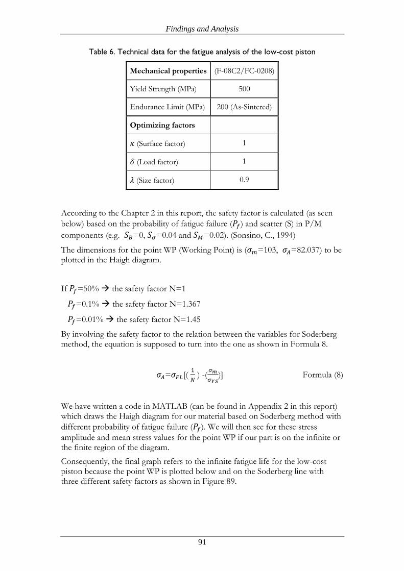
Findings and Analysis
91
Table 6. Technical data for the fatigue analysis of the low-cost piston
Mechanical properties (F-08C2/FC-0208)
Yield Strength (MPa) 500
Endurance Limit (MPa) 200 (As-Sintered)
Optimizing factors
(Surface factor) 1
(Load factor) 1
(Size factor) 0.9
According to the Chapter 2 in this report, the safety factor is calculated (as seen
below) based on the probability of fatigue failure ( ) and scatter (S) in P/M
components (e.g. =0, =0.04 and =0.02). (Sonsino, C., 1994)
The dimensions for the point WP (Working Point) is ( =103, =82.037) to be plotted in the Haigh diagram.
If =50% the safety factor N=1
=0.1% the safety factor N=1.367
=0.01% the safety factor N=1.45
By involving the safety factor to the relation between the variables for Soderberg method, the equation is supposed to turn into the one as shown in Formula 8.
= [( 1
) -(
)] Formula (8)
We have written a code in MATLAB (can be found in Appendix 2 in this report) which draws the Haigh diagram for our material based on Soderberg method with
different probability of fatigue failure ( ). We will then see for these stress
amplitude and mean stress values for the point WP if our part is on the infinite or the finite region of the diagram.
Consequently, the final graph refers to the infinite fatigue life for the low-cost piston because the point WP is plotted below and on the Soderberg line with three different safety factors as shown in Figure 89.
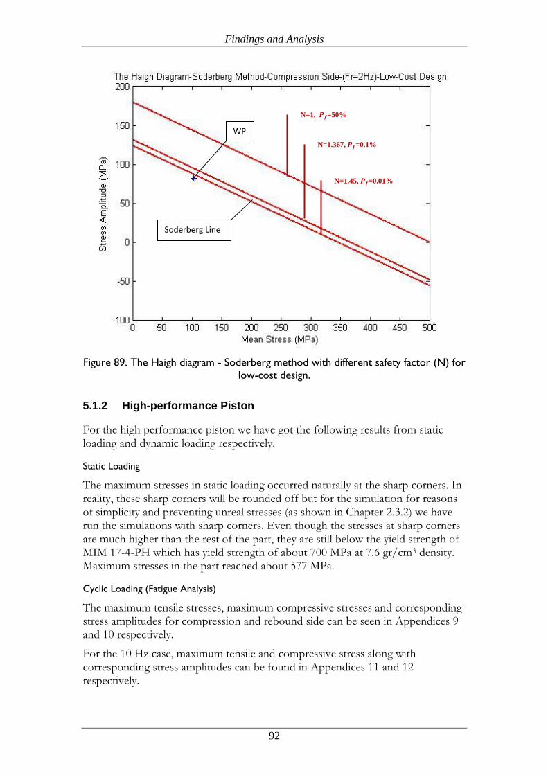
Findings and Analysis
92
Figure 89. The Haigh diagram - Soderberg method with different safety factor (N) for
low-cost design.
5.1.2 High-performance Piston
For the high performance piston we have got the following results from static loading and dynamic loading respectively.
Static Loading
The maximum stresses in static loading occurred naturally at the sharp corners. In reality, these sharp corners will be rounded off but for the simulation for reasons of simplicity and preventing unreal stresses (as shown in Chapter 2.3.2) we have run the simulations with sharp corners. Even though the stresses at sharp corners are much higher than the rest of the part, they are still below the yield strength of MIM 17-4-PH which has yield strength of about 700 MPa at 7.6 gr/cm3 density. Maximum stresses in the part reached about 577 MPa.
Cyclic Loading (Fatigue Analysis)
The maximum tensile stresses, maximum compressive stresses and corresponding stress amplitudes for compression and rebound side can be seen in Appendices 9 and 10 respectively.
For the 10 Hz case, maximum tensile and compressive stress along with corresponding stress amplitudes can be found in Appendices 11 and 12 respectively.
N=1.45, 𝑷𝒇=0.01%
N=1.367, 𝑷𝒇=0.1%
N=1, 𝑷𝒇=50%
Soderberg Line
WP
Findings and Analysis
93
It can been seen easily that on the rebound side stress ranges are much lower than on the compression side, therefore we will make our fatigue life estimation based on the results from the compression side with the frequency of 2 Hz.
Based on these results, the maximum local stress range is at element number 275046 (out of a total number of 478309 elements for FEM analysis with Abaqus)
which has a stress amplitude ( ) 89.020 MPa and a mean stress ( ) with the value of 97 MPa.
Fatigue Life Analysis
As already discussed in the Chapter 2 in this report, the fatigue life estimation is calculated based on the optimized fatigue endurance. The mechanical properties for the selected MIM powder material (MIM-17-4 PH) are shown in Table 7. The
endurance limit can be determined by dividing the ultimate tensile strength ( ) by the ratio of 0.315 (as an average for P/M part) for the high performance design in this project because there are no fatigue properties for MIM P/M parts. (O'Brien, R. C. 1988)
The endurance limit for MIM-17-4 PH = 0.315* =283.5 MPa
Similar to the low-cost design, to predict the fatigue life for the high-performance piston, the Haigh diagram with Soderberg method can be used. Note that the fatigue endurance and Soderberg line will be optimized by all optimizing factors and the safety factor almost the similar to the low-cost design in the previous chapter as seen in Table 7. All factors may be determined from the mechanical engineer’s handbooks. (Marghitu, D. B., 2001)
According to the standard tests, it was revealed that the load factor ( ) for bending
load is one. Since the surface finish for MIM parts is almost 0.8 , it may be estimated for factor ( ) is also given the value of 0.75, and the value for the last
factor is 0.9. (Marghitu, D. B., 2001, and epma.com)
The optimized fatigue endurance (Opt. )= . . .
=283.5 MPa Opt. =191.36MPa
Similarly, the safety factors are calculated based on the different probabilities of
fatigue failure ( ) and scatters (S) in MIM components nearly similar to
Conventional Sinter and Pressing parts. The dimensions for the point WP
(Working Point) for high-performance piston are ( =97, =89.020) to be plotted in the Haigh diagram as depicted in Figure 90.
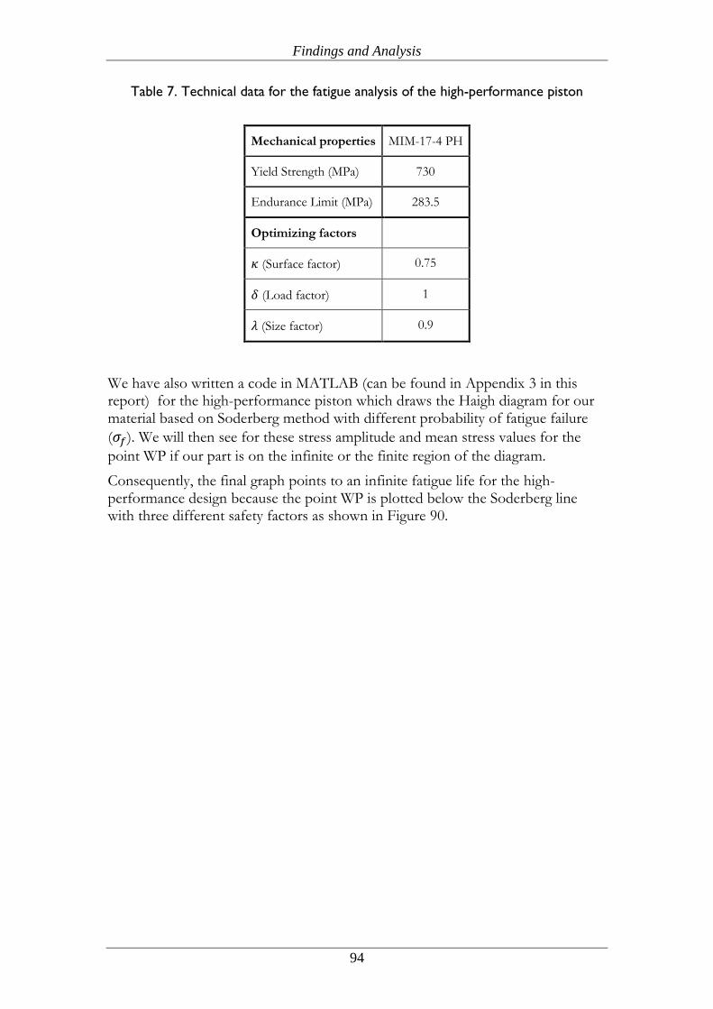
Findings and Analysis
94
Table 7. Technical data for the fatigue analysis of the high-performance piston
Mechanical properties MIM-17-4 PH
Yield Strength (MPa) 730
Endurance Limit (MPa) 283.5
Optimizing factors
(Surface factor) 0.75
(Load factor) 1
(Size factor) 0.9
We have also written a code in MATLAB (can be found in Appendix 3 in this report) for the high-performance piston which draws the Haigh diagram for our material based on Soderberg method with different probability of fatigue failure
( ). We will then see for these stress amplitude and mean stress values for the
point WP if our part is on the infinite or the finite region of the diagram.
Consequently, the final graph points to an infinite fatigue life for the high-performance design because the point WP is plotted below the Soderberg line with three different safety factors as shown in Figure 90.
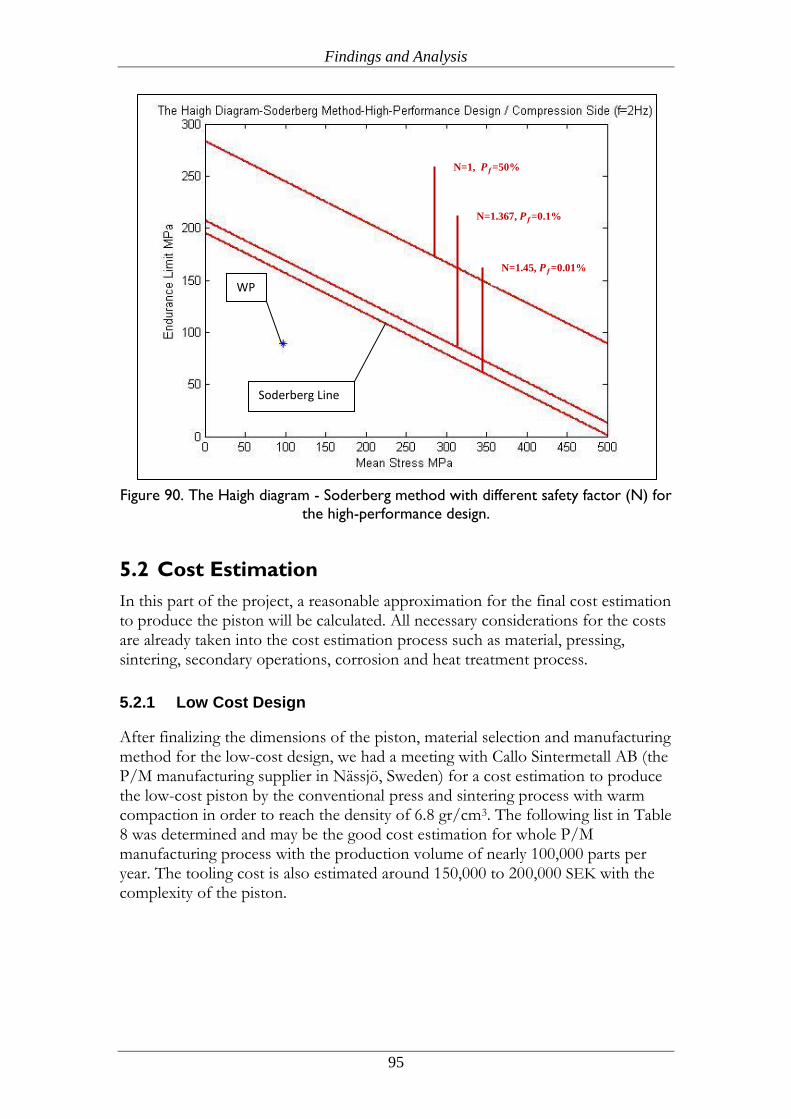
Findings and Analysis
95
Figure 90. The Haigh diagram - Soderberg method with different safety factor (N) for
the high-performance design.
5.2 Cost Estimation
In this part of the project, a reasonable approximation for the final cost estimation to produce the piston will be calculated. All necessary considerations for the costs are already taken into the cost estimation process such as material, pressing, sintering, secondary operations, corrosion and heat treatment process.
5.2.1 Low Cost Design
After finalizing the dimensions of the piston, material selection and manufacturing method for the low-cost design, we had a meeting with Callo Sintermetall AB (the P/M manufacturing supplier in Nässjö, Sweden) for a cost estimation to produce the low-cost piston by the conventional press and sintering process with warm compaction in order to reach the density of 6.8 gr/cm3. The following list in Table 8 was determined and may be the good cost estimation for whole P/M manufacturing process with the production volume of nearly 100,000 parts per year. The tooling cost is also estimated around 150,000 to 200,000 SEK with the complexity of the piston.
N=1.45, 𝑷𝒇=0.01%
N=1.367, 𝑷𝒇=0.1%
N=1, 𝑷𝒇=50%
Soderberg Line
WP
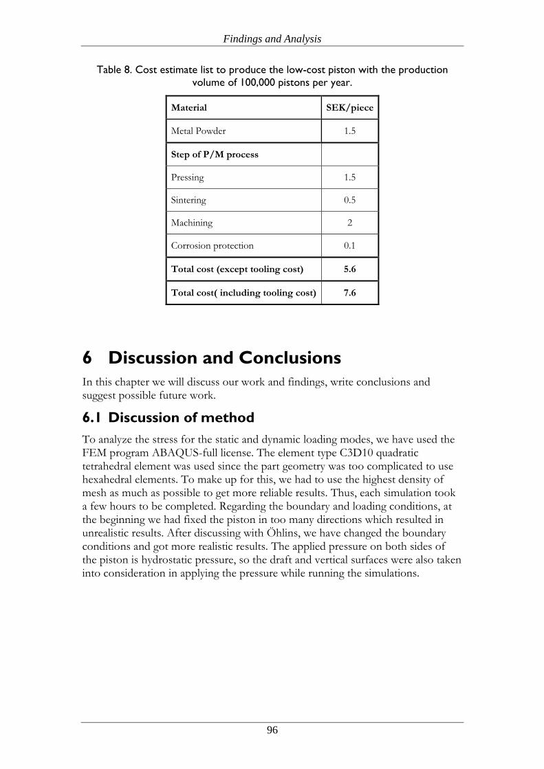
Findings and Analysis
96
Table 8. Cost estimate list to produce the low-cost piston with the production
volume of 100,000 pistons per year.
Material SEK/piece
Metal Powder 1.5
Step of P/M process
Pressing 1.5
Sintering 0.5
Machining 2
Corrosion protection 0.1
Total cost (except tooling cost) 5.6
Total cost( including tooling cost) 7.6
6 Discussion and Conclusions
In this chapter we will discuss our work and findings, write conclusions and suggest possible future work.
6.1 Discussion of method
To analyze the stress for the static and dynamic loading modes, we have used the FEM program ABAQUS-full license. The element type C3D10 quadratic tetrahedral element was used since the part geometry was too complicated to use hexahedral elements. To make up for this, we had to use the highest density of mesh as much as possible to get more reliable results. Thus, each simulation took a few hours to be completed. Regarding the boundary and loading conditions, at the beginning we had fixed the piston in too many directions which resulted in unrealistic results. After discussing with Öhlins, we have changed the boundary conditions and got more realistic results. The applied pressure on both sides of the piston is hydrostatic pressure, so the draft and vertical surfaces were also taken into consideration in applying the pressure while running the simulations.
Search terms
97
To carry out the fatigue failure analysis for dynamic loads, the frequencies were not considered. The first reason was lack of enough data for plastic material properties of P/M parts, and another reason was too much computational time to run the simulations in ABAQUS. First, we tried to analyze the cyclic load using a Direct Cyclic Step in ABAQUS. Although it was complicated to set up a varying load condition provided by Öhlins, we managed to make a simulation consisting of three cycles. However, such simulation took several hours to be completed even with only three cycles. To make a high cycle fatigue analysis, one needs to run a simulation with at least 100,000 cycles which would take a very long time in this case. We also needed plastic material data which we did not have. After discussing this with our supervisor based on his suggestions we have changed our approach for fatigue failure analysis and followed a more straightforward method in which we carried out the simulation statically and located the maximum stress amplitudes and corresponding mean stresses to see where the most critical areas are. Finally, Haigh diagram was accepted to carry out the calculations. Among different methods for plotting the Haigh diagram like Geber Parabolic, Goodman and Soderberg , eventually Soderberg technique was selected to predict fatigue life for both designs because this method was able to fulfill the technical requirements of the piston such as no plastic deformation on the piston during normal working conditions and estimation of an infinite fatigue life. In this case, the limit on
abscissa for the mean stress is less than yield strength ( ) and on ordinate for the
fatigue endurance ( ), so this line is called Soderberg line.
6.2 Discussion of findings
The purpose of the thesis was to investigate the possibility of redesigning this shock absorber piston so that it can be manufactured by sintering process and still keep the same performance.
We will restate our research questions and answer them.
How can this currently machined shock absorber piston be redesigned and developed for powder metallurgy process, so that it fulfills the technical requirements associated with it?
Search terms
98
We have followed the design guidelines for each manufacturing method (Conventional Press and Sintering & Metal Injection Molding) and redesigned the piston both according to these guidelines and the preset requirements of the shock absorber piston. We have made the wall thicknesses thicker, changed the shape of the through holes to make them as big as possible, merged the six different areas on the piston into one big area but kept the total area almost the same which is important for the performance of the piston. For the low-cost design we have made the height of the piston longer than the original piston in order to make up for the porous material and the lower mechanical properties associated with it. After carrying out the FEM simulations we have seen that both designs can withstand the applied forces while fulfilling the dimensional requirements. They were also designed with the economic issues and cheaper production taken into consideration. Next step would be to make a prototype and test the piston under real working conditions to see how it performs.
What approach would be more reliable to estimate the fatigue life for a P/M part?
The constant stress amplitude and no plastic deformation on the piston during the real working conditions were the most important requirements to choose the Haigh diagram with Soderberg method to analyze the fatigue failure. Other issues like having an infinite number of cycles of fatigue life and including the optimizing factors to determine the real fatigue endurance of materials led us to use the Haigh diagram technique to estimate fatigue life.
6.3 Conclusions
Two different shock absorber piston designs have been created to be manufactured by two different processes: Conventional Powder Metallurgy with warm compaction and Metal Injection Molding.
Suggested material for the low-cost design is F-08C2/FC-0208. However, 306L and 316L can also be considered depending on the elongation.
For the low-cost design, machining and corrosion protection are needed after sintering. Heat treatment might be necessary if the selected material is 306L or 316L in order to increase the strength.
Stress analysis results show that stresses in the low-cost design do not exceed the yield strength of the material F-08C2/FC-0208. Based on Soderberg approach and the given dynamic loading conditions, the part is safe regarding the fatigue life as well.
For the high performance piston, MIM-17-4 PH is a good option, providing high strength, moderate ductility and corrosion resistance. Heat treated MIM 2700 has also good mechanical properties but prices need to be investigated because of the heat treatment process.
Search terms
99
FEM analysis of the high performance piston showed that the maximum stress amplitude in the piston is under the Soderberg line by far which means it is in the safe region regarding fatigue life.
It must be kept in mind that prototypes need to be produced and tested under real working conditions. Finite element analysis includes some approximations and only gives an idea about the expected stress levels in the product.
6.4 Future work
Prototypes should be manufactured and tested under working conditions.
The frequency effects of the dynamic loading can be taken into consideration.
Simulations can be run on a computer with more memory in order to increase the number of elements and the accuracy of the results.
Parts can be meshed via a pre-processing tool (such as HyperMesh) so that quadratic hexahedral elements can be used in the simulations, leading to increased accuracy.
Further design changes can be made and simulations can be re-run in an iterative process to reach an optimal design.
Topology optimization can be the next step to get an optimal design for both pistons especially for the high-performance piston with very expensive powder metal.
Search terms
100
7 References
ABAQUS Analysis User’s Manual, Part V: Materials, Chapter 18.3.1 Elastic Behaviour of Porous Materials
Babakhani, A., Haerian, A., Ghambari, M. (2006) On the combined effect of lubrication and compaction temperature on properties of iron-based P/M parts. Materials Science and Engineering A 437 (2006) 360-365
Beiss, P. (2007) Functional Relationships between Fatigue Data. Design and Capabilities of PM Components and Materials, 2007 EPMA Powder Course Figures Vol 1.
Benzley, S. E., Perry, E., Merkley, K., Clark, B. (1995) A Comparison of All Hexagonal and All Tetrahedral Finite Element Meshes for Elastic and Elasto-plastic Analysis. Proceedings, 4th International Meshing Roundtable, Sandia National Laboratories. Pages 179-191
Black, J. T., Kohser, R. A. (2008) DeGarmo’s Materials & Processes In Manufacturing. John Wiley & Sons Inc.
Cifuentes, A. O., Kalbag, A. (1992) A performance study of tetrahedral and hexahedral elements in 3-D finite element structural analysis. Finite Elements in Analysis and Design 12 (1992) Pages 313-318
Dahlberg, T., Ekberg, A., (2002) Failure Fracture Fatigue: An introduction. Studentlitteratur, Lund
European Powder Metallurgy Association http://www.epma.com (Acc. 8 May 2012)
Farjoud, A., Ahmadian, M., Craft, M., Burke, W. (2012) Nonlinear modelling and experimental characterization of hydraulic dampers: effects of shim stack and orifice parameters on damper performance. Nonlinear Dynamics Volume 67 Number 2 DOI: 10.1007/s11071-011-0079-2
German, M. R. (1994) Powder Metallurgy Science. 2nd ed. Metal Powder Industry, New Jersey
Höganäs, (2004) Höganäs Handbook for Warm Compaction. Höganäs AB, Sweden (http://www.hoganas.com)
Höganäs, (2007) Höganäs Handbook for Design and Mechanical Properties. Höganäs AB, Sweden (http://www.hoganas.com)
Jian-hong, Y., Tu-ming, Y., Yuan-dong, P., Qing-lin, X., Hong-zhong, W. (2007) Effects of warm compaction on mechanical properties of sintered P/M steels. DOI: 10.1007/s11771-007-0087-z
Kennedy, D. (2003) Shock Q&A. Chassis & Suspension Handbook. HP Books, New York
Search terms
101
Kinetics (2004) Kinetics MIM Design Guide. Kinetics Metal Injection Molding, USA. (http://www.kinetics.com)
Leonelli, C., Veronesi, P., Denti, L., Gatto, A., Iuliano, L. (2008) Microwave assisted sintering of green metal parts. Journal of Materials Processing Technology Volume 205, Issues 1-3, 26 August 2008, Pages 489-496
Marghitu, D. B. (2001) Mechanical Engineer’s Handbook. Academic Press, San Diego, California
National Research Council (U.S.) (1994) Microwave Processing of Materials. National Academy Press, Washington
Negari, M. N. A., Mamoory, R. S., Simchi, A., Ehsani, N. (2007) Determination of the Physical and Mechanical Properties of Iron-based Powder Materials Produced by Microwave Sintering. Powder Metallurgy and Metal Ceramics, Vol. 46, Nos. 9-10, 2007
O'Brien, R. C. (1988) Fatigue Properties of P/M Materials. Höganäs Corporation. The SAE Congress, Detroit, Michigan
Öhlins Racing AB http://www.ohlins.com (Acc.8 May 2012)
R. K. Holman, P.K. Liaw, (1997) Methodologies for Predicting Fatigue Life. TMS (Minerals, Metals & Materials Society) Fall Extraction & Processing Conference, Royal Sonesta, Cambridge, Massachusetts.
Shepherd, J. F., Johnson, C. R. (2008) Hexahedral Mesh Generation Constraints. Engineering with Computers 24, Pages 195-213
Sonsino, C. M., Esper, F. J. (1994) Fatigue Design for PM Components. European Powder Metallurgy Association, Shrewsbury
Stolt, R. (2008) CAD-Model Parsing for Automated Design and Design Evaluation. Chalmers University of Technology, Göteborg
Veyhl, C., Belova, I.V., Murch, G. E., Öchsner, A., Fiedler, T. (2010) On the mesh dependence of non-linear mechanical finite element analysis. Finite Elements in Analysis and Design 46 (2010) Pages 371-378
Wang, E., Nelson, T., Rauch, R. (2004) Back to Elements-Tetrahedra vs. Hexahedra. International ANSYS Conference Proceedings 2004
Yalcin, B., Ucun, I., Usal, M.R. (2009) Failure Analysis of a Shock Absorber Piston Produced by Powder Metallurgy Processing. 5th International Advanced Technologies Symposium 2009
Yuandong, P., Jianhong, Y., Shudong, L., Yingli, G., Liya, L. (2009) Microstructure Analysis of Microwave Sintered Ferrous PM Alloys. Journal of Wuhan University of Technology Materials Science Edition Volume 24, Number 2 (2009), DOI: 10.1007/s11595-009-2214-1
Appendices
102
8 Appendices
Appendix 1. Drawing technical sheet of piston for the low-cost design
Appendix 2. Matlab code for the Haigh diagram for low cost design
Appendix 3. Matlab code for the Haigh diagram for high performance design
Appendix 4. Drawing technical sheet of piston for the high-performance design
Appendix 5. Maximum stress values (Case: 2 Hz, Compression side)
Appendix 6. Maximum stress values (Case: 2 Hz, Rebound side)
Appendix 7. Maximum stress values (Case: 10 Hz, Compression side)
Appendix 8. Maximum stress values (Case: 10 Hz, Rebound side)
Appendix 9. Maximum stress values (Case: 2 Hz, Compression side)
Appendix 10. Maximum stress values (Case: 2 Hz, Rebound side)
Appendix 11. Maximum stress values (Case: 10 Hz, Compression side)
Appendix 12. Maximum stress values (Case: 10 Hz, Rebound side)
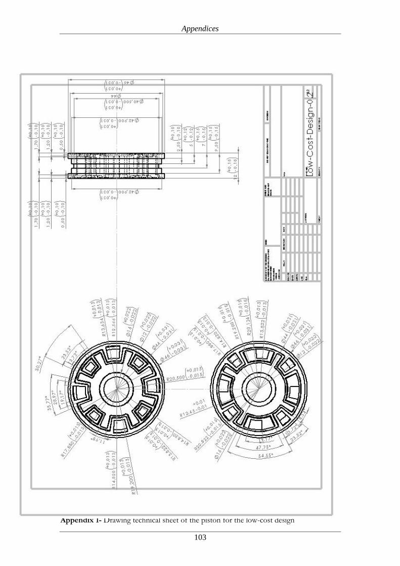
Appendices
103
Appendix 1- Drawing technical sheet of the piston for the low-cost design
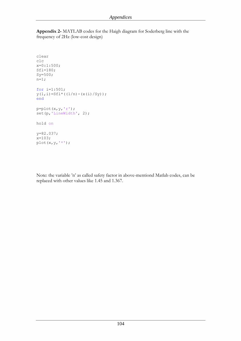
Appendices
104
Appendix 2- MATLAB codes for the Haigh diagram for Soderberg line with the frequency of 2Hz (low-cost design)
clear clc x=0:1:500; Sfl=180; Sy=500; n=1;
for i=1:501; y(1,i)=Sfl*((1/n)-(x(i)/Sy)); end
p=plot(x,y,'r'); set(p,'LineWidth', 2);
hold on
y=82.037; x=103; plot(x,y,'*');
Note: the variable ’n’ as called safety factor in above-mentiond Matlab codes, can be replaced with other values like 1.45 and 1.367.
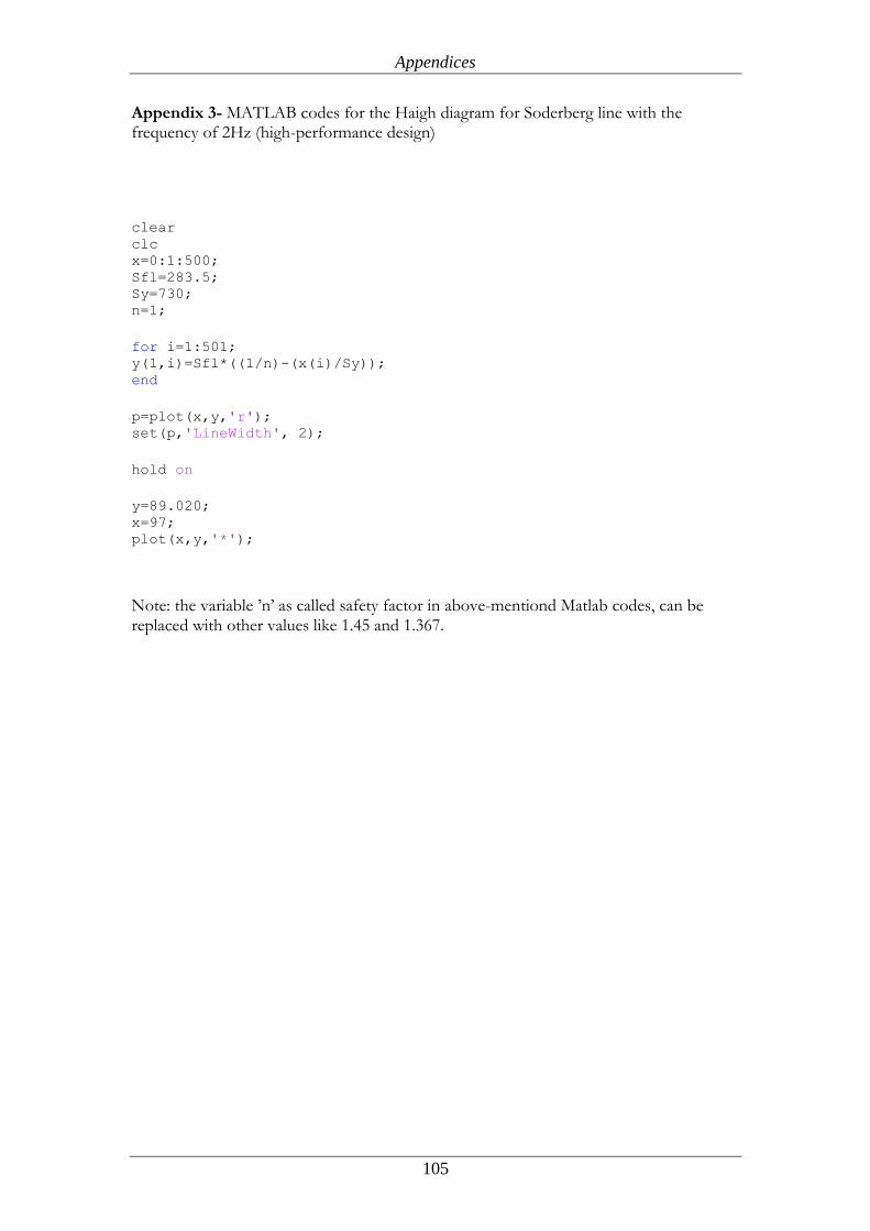
Appendices
105
Appendix 3- MATLAB codes for the Haigh diagram for Soderberg line with the frequency of 2Hz (high-performance design)
clear clc x=0:1:500; Sfl=283.5; Sy=730; n=1;
for i=1:501; y(1,i)=Sfl*((1/n)-(x(i)/Sy)); end
p=plot(x,y,'r'); set(p,'LineWidth', 2);
hold on
y=89.020; x=97; plot(x,y,'*');
Note: the variable ’n’ as called safety factor in above-mentiond Matlab codes, can be replaced with other values like 1.45 and 1.367.
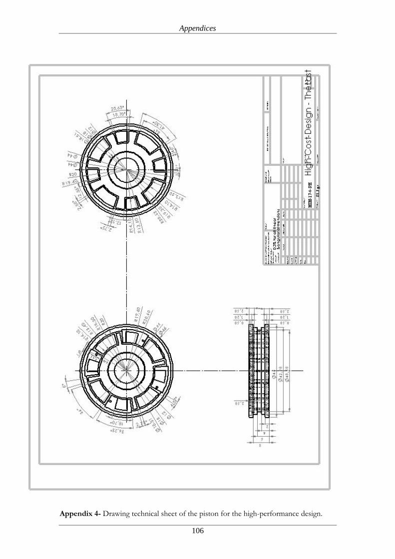
Appendices
106
Appendix 4- Drawing technical sheet of the piston for the high-performance design.
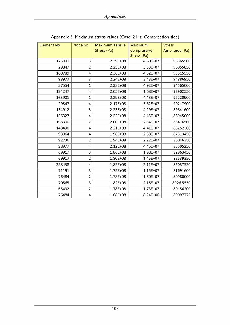
Appendices
107
Appendix 5. Maximum stress values (Case: 2 Hz, Compression side)
Element No Node no Maximum Tensile Stress (Pa)
Maximum Compressive Stress (Pa)
Stress Amplitude (Pa)
125091 3 2.39E+08 4.60E+07 96365500
29847 2 2.25E+08 3.33E+07 96055850
160789 4 2.36E+08 4.52E+07 95515550
98977 3 2.24E+08 3.43E+07 94886950
37554 1 2.38E+08 4.92E+07 94565000
124247 4 2.05E+08 1.68E+07 93902550
165901 1 2.29E+08 4.43E+07 92220900
29847 4 2.17E+08 3.62E+07 90217900
134912 3 2.23E+08 4.29E+07 89841600
136327 4 2.22E+08 4.45E+07 88945000
198300 2 2.00E+08 2.34E+07 88476500
148490 4 2.21E+08 4.41E+07 88252300
93064 4 1.98E+08 2.38E+07 87313450
92736 2 1.94E+08 2.22E+07 86046350
98977 4 2.12E+08 4.45E+07 83595250
69917 3 1.86E+08 1.98E+07 82963450
69917 2 1.80E+08 1.45E+07 82539350
258438 4 1.85E+08 2.11E+07 82037550
71191 3 1.75E+08 1.15E+07 81691600
76484 2 1.78E+08 1.60E+07 80980000
70565 3 1.82E+08 2.15E+07 8026 5550
65492 2 1.78E+08 1.73E+07 80156200
76484 4 1.68E+08 8.24E+06 80097775
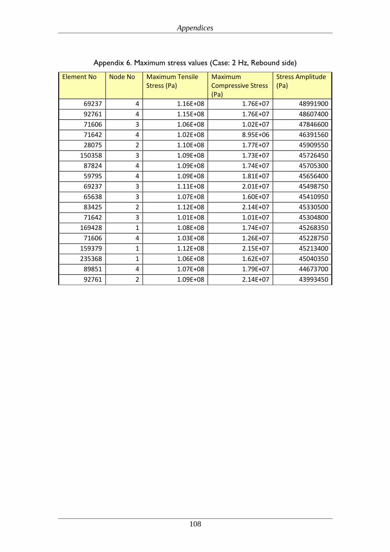
Appendices
108
Appendix 6. Maximum stress values (Case: 2 Hz, Rebound side)
Element No Node No Maximum Tensile Stress (Pa)
Maximum Compressive Stress (Pa)
Stress Amplitude (Pa)
69237 4 1.16E+08 1.76E+07 48991900
92761 4 1.15E+08 1.76E+07 48607400
71606 3 1.06E+08 1.02E+07 47846600
71642 4 1.02E+08 8.95E+06 46391560
28075 2 1.10E+08 1.77E+07 45909550
150358 3 1.09E+08 1.73E+07 45726450
87824 4 1.09E+08 1.74E+07 45705300
59795 4 1.09E+08 1.81E+07 45656400
69237 3 1.11E+08 2.01E+07 45498750
65638 3 1.07E+08 1.60E+07 45410950
83425 2 1.12E+08 2.14E+07 45330500
71642 3 1.01E+08 1.01E+07 45304800
169428 1 1.08E+08 1.74E+07 45268350
71606 4 1.03E+08 1.26E+07 45228750
159379 1 1.12E+08 2.15E+07 45213400
235368 1 1.06E+08 1.62E+07 45040350
89851 4 1.07E+08 1.79E+07 44673700
92761 2 1.09E+08 2.14E+07 43993450
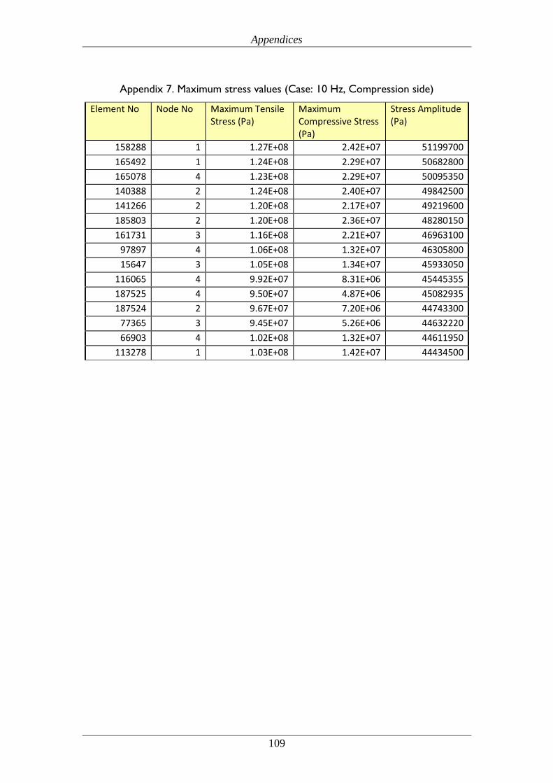
Appendices
109
Appendix 7. Maximum stress values (Case: 10 Hz, Compression side)
Element No Node No Maximum Tensile Stress (Pa)
Maximum Compressive Stress (Pa)
Stress Amplitude (Pa)
158288 1 1.27E+08 2.42E+07 51199700
165492 1 1.24E+08 2.29E+07 50682800
165078 4 1.23E+08 2.29E+07 50095350
140388 2 1.24E+08 2.40E+07 49842500
141266 2 1.20E+08 2.17E+07 49219600
185803 2 1.20E+08 2.36E+07 48280150
161731 3 1.16E+08 2.21E+07 46963100
97897 4 1.06E+08 1.32E+07 46305800
15647 3 1.05E+08 1.34E+07 45933050
116065 4 9.92E+07 8.31E+06 45445355
187525 4 9.50E+07 4.87E+06 45082935
187524 2 9.67E+07 7.20E+06 44743300
77365 3 9.45E+07 5.26E+06 44632220
66903 4 1.02E+08 1.32E+07 44611950
113278 1 1.03E+08 1.42E+07 44434500
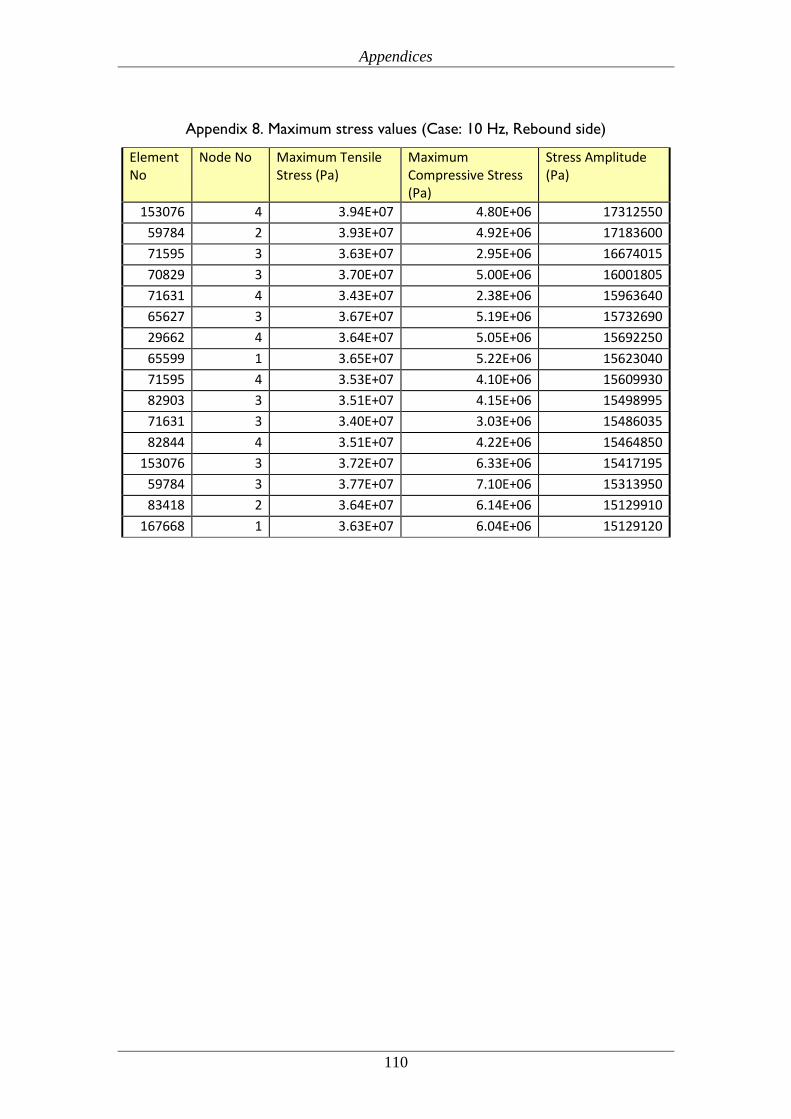
Appendices
110
Appendix 8. Maximum stress values (Case: 10 Hz, Rebound side)
Element No
Node No Maximum Tensile Stress (Pa)
Maximum Compressive Stress (Pa)
Stress Amplitude (Pa)
153076 4 3.94E+07 4.80E+06 17312550
59784 2 3.93E+07 4.92E+06 17183600
71595 3 3.63E+07 2.95E+06 16674015
70829 3 3.70E+07 5.00E+06 16001805
71631 4 3.43E+07 2.38E+06 15963640
65627 3 3.67E+07 5.19E+06 15732690
29662 4 3.64E+07 5.05E+06 15692250
65599 1 3.65E+07 5.22E+06 15623040
71595 4 3.53E+07 4.10E+06 15609930
82903 3 3.51E+07 4.15E+06 15498995
71631 3 3.40E+07 3.03E+06 15486035
82844 4 3.51E+07 4.22E+06 15464850
153076 3 3.72E+07 6.33E+06 15417195
59784 3 3.77E+07 7.10E+06 15313950
83418 2 3.64E+07 6.14E+06 15129910
167668 1 3.63E+07 6.04E+06 15129120
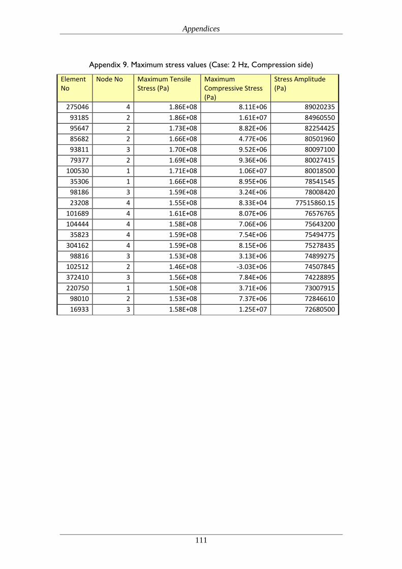
Appendices
111
Appendix 9. Maximum stress values (Case: 2 Hz, Compression side)
Element No
Node No Maximum Tensile Stress (Pa)
Maximum Compressive Stress (Pa)
Stress Amplitude (Pa)
275046 4 1.86E+08 8.11E+06 89020235
93185 2 1.86E+08 1.61E+07 84960550
95647 2 1.73E+08 8.82E+06 82254425
85682 2 1.66E+08 4.77E+06 80501960
93811 3 1.70E+08 9.52E+06 80097100
79377 2 1.69E+08 9.36E+06 80027415
100530 1 1.71E+08 1.06E+07 80018500
35306 1 1.66E+08 8.95E+06 78541545
98186 3 1.59E+08 3.24E+06 78008420
23208 4 1.55E+08 8.33E+04 77515860.15
101689 4 1.61E+08 8.07E+06 76576765
104444 4 1.58E+08 7.06E+06 75643200
35823 4 1.59E+08 7.54E+06 75494775
304162 4 1.59E+08 8.15E+06 75278435
98816 3 1.53E+08 3.13E+06 74899275
102512 2 1.46E+08 -3.03E+06 74507845
372410 3 1.56E+08 7.84E+06 74228895
220750 1 1.50E+08 3.71E+06 73007915
98010 2 1.53E+08 7.37E+06 72846610
16933 3 1.58E+08 1.25E+07 72680500
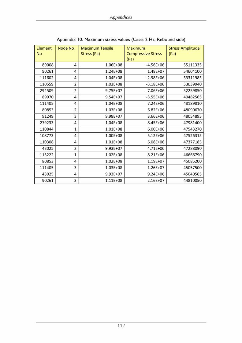
Appendices
112
Appendix 10. Maximum stress values (Case: 2 Hz, Rebound side)
Element No
Node No Maximum Tensile Stress (Pa)
Maximum Compressive Stress (Pa)
Stress Amplitude (Pa)
89008 4 1.06E+08 -4.56E+06 55111335
90261 4 1.24E+08 1.48E+07 54604100
111602 4 1.04E+08 -2.98E+06 53311985
110559 2 1.03E+08 -3.18E+06 53039940
294509 2 9.75E+07 -7.06E+06 52259850
89970 4 9.54E+07 -3.55E+06 49482565
111405 4 1.04E+08 7.24E+06 48189810
80853 2 1.03E+08 6.82E+06 48090670
91249 3 9.98E+07 3.66E+06 48054895
279233 4 1.04E+08 8.45E+06 47981400
110844 1 1.01E+08 6.00E+06 47543270
108773 4 1.00E+08 5.12E+06 47526315
110308 4 1.01E+08 6.08E+06 47377185
43025 2 9.93E+07 4.71E+06 47288090
113222 1 1.02E+08 8.21E+06 46666790
80853 4 1.02E+08 1.19E+07 45085200
111405 3 1.03E+08 1.26E+07 45057500
43025 4 9.93E+07 9.24E+06 45040565
90261 3 1.11E+08 2.16E+07 44810050
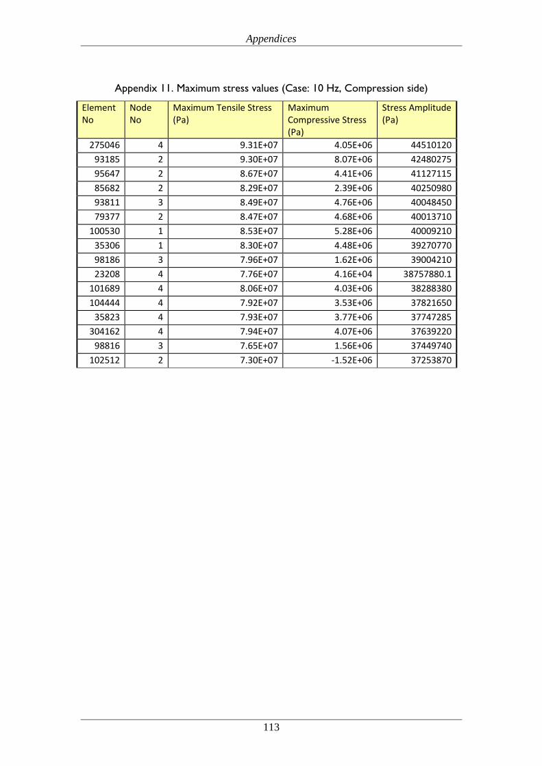
Appendices
113
Appendix 11. Maximum stress values (Case: 10 Hz, Compression side)
Element No
Node No
Maximum Tensile Stress (Pa)
Maximum Compressive Stress (Pa)
Stress Amplitude (Pa)
275046 4 9.31E+07 4.05E+06 44510120
93185 2 9.30E+07 8.07E+06 42480275
95647 2 8.67E+07 4.41E+06 41127115
85682 2 8.29E+07 2.39E+06 40250980
93811 3 8.49E+07 4.76E+06 40048450
79377 2 8.47E+07 4.68E+06 40013710
100530 1 8.53E+07 5.28E+06 40009210
35306 1 8.30E+07 4.48E+06 39270770
98186 3 7.96E+07 1.62E+06 39004210
23208 4 7.76E+07 4.16E+04 38757880.1
101689 4 8.06E+07 4.03E+06 38288380
104444 4 7.92E+07 3.53E+06 37821650
35823 4 7.93E+07 3.77E+06 37747285
304162 4 7.94E+07 4.07E+06 37639220
98816 3 7.65E+07 1.56E+06 37449740
102512 2 7.30E+07 -1.52E+06 37253870
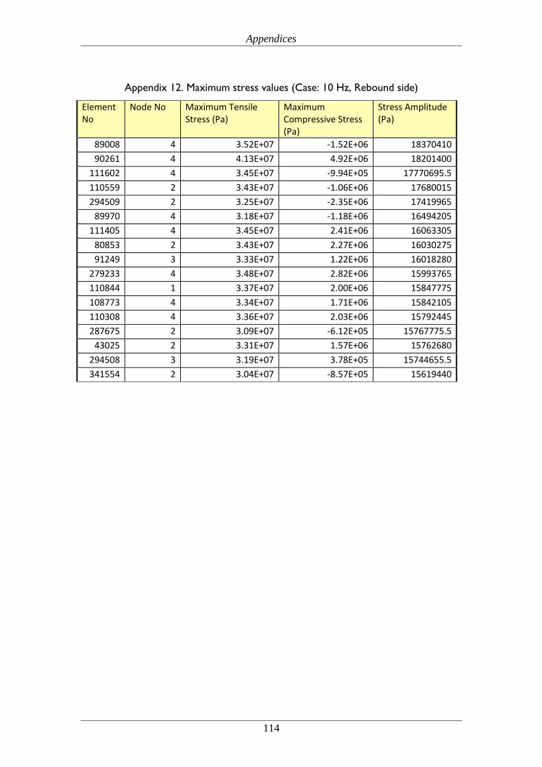
Appendices
114
Appendix 12. Maximum stress values (Case: 10 Hz, Rebound side)
Element No
Node No Maximum Tensile Stress (Pa)
Maximum Compressive Stress (Pa)
Stress Amplitude (Pa)
89008 4 3.52E+07 -1.52E+06 18370410
90261 4 4.13E+07 4.92E+06 18201400
111602 4 3.45E+07 -9.94E+05 17770695.5
110559 2 3.43E+07 -1.06E+06 17680015
294509 2 3.25E+07 -2.35E+06 17419965
89970 4 3.18E+07 -1.18E+06 16494205
111405 4 3.45E+07 2.41E+06 16063305
80853 2 3.43E+07 2.27E+06 16030275
91249 3 3.33E+07 1.22E+06 16018280
279233 4 3.48E+07 2.82E+06 15993765
110844 1 3.37E+07 2.00E+06 15847775
108773 4 3.34E+07 1.71E+06 15842105
110308 4 3.36E+07 2.03E+06 15792445
287675 2 3.09E+07 -6.12E+05 15767775.5
43025 2 3.31E+07 1.57E+06 15762680
294508 3 3.19E+07 3.78E+05 15744655.5
341554 2 3.04E+07 -8.57E+05 15619440