Redalyc.A New Stability Analysis Method for DC to … · A New Stability Analysis Method for DC to DC Series Resonant Converters ... puramente geométricas en lugar de los eigenvalores

Computación y Sistemas

ISSN: 1405-5546

[email protected]

Instituto Politécnico Nacional

México

Hernández Guzmán, Victor

A New Stability Analysis Method for DC to DC Series Resonant Converters

Computación y Sistemas, vol. 11, núm. 1, julio-septiembre, 2007, pp. 14-25

Instituto Politécnico Nacional

Distrito Federal, México

Available in: http://www.redalyc.org/articulo.oa?id=61511103

How to cite

Complete issue

More information about this article

Journal's homepage in redalyc.org

Scientific Information System

Network of Scientific Journals from Latin America, the Caribbean, Spain and Portugal

Non-profit academic project, developed under the open access initiative

http://www.redalyc.org/revista.oa?id=615

http://www.redalyc.org/articulo.oa?id=61511103

http://www.redalyc.org/comocitar.oa?id=61511103

http://www.redalyc.org/fasciculo.oa?id=615&numero=10129

http://www.redalyc.org/articulo.oa?id=61511103

http://www.redalyc.org/revista.oa?id=615

http://www.redalyc.org

A New Stability Analysis Method for DC to DC Series Resonant Converters Un Nuevo Método para el Análisis de Estabilidad de Convertidores Resonantes Serie de CD a CD.

Victor Hernández Guzmán

Universidad Autónoma de Querétaro, Facultad de Ingeniería. A.P. 3-24, C.P. 76150. Querétaro, Qro., México.

[email protected]

Article received on July 19, 2006; accepted on October 01, 2007

Abstract In this note we present a novel stability analysis method for DC to DC series resonant converters which relies on the phase plane technique. This method gives more insight into the rationale behind the stability conditions because these are obtained from geometrical considerations instead of eigenvalues of linear discrete time approximations as presented in previous works. The proposed method allows to understand easily how the performance is affected as the location of the operating point changes on the phase plane which is not an easy task when previously proposed methods are used. We show how to use numerical computations, based on this stability analysis method, to determine graphically the region of the phase plane where asymptotically stable closed trajectories exist. Further, a nice geometrical condition is formulated to achieve the fastest convergence rate to the closed trajectory under study. Keywords: Stability, Control of series resonant converters, Phase plane analysis.

Resumen En este trabajo se presenta un nuevo método para el análisis de estabilidad de convertidores resonantes serie de CD a CD que se basa en al descripción del convertidor en el plano de fase. Este método facilita la comprensión del problema y de las condiciones que establecen su solución porque éstas son obtenidas a partir de consideraciones puramente geométricas en lugar de los eigenvalores de aproximaciones lineales en tiempo discreto como ha sido reportado en trabajos previos. Este método también facilita comprender como el desempeño del convertidor es afectado al cambiar la ubicación en el plano de fase del punto de operación, lo cual no es sencillo de determinar usando los métodos propuestos previamente. Se muestra como se pueden hacer cálculos numéricos, basados en este método, para determinar de manera gráfica la región del plano de fase donde existen trayectorias cerradas asintóticamente estables. También se establece una condición geométrica para obtener la tasa de convergencia más rápida a la trayectoria cerrada bajo estudio. Palabras clave: Estabilidad, Control de convertidores resonantes serie, Análisis en el plano de fase.

1 Introduction

The phase plane technique has shown to be a powerful tool for analysis and design of DC to DC series resonant converters since it was introduced by Oruganti and Lee (1985). Based on these ideas an optimal trajectory controller was presented by Oruganti and Lee (1985) and Oruganti et al. (1988) which transfers the converter from one operating point to another in a minimal interval of time. Further, two innovative controllers were presented by Kim et al. (1991) and Kim and Youn (1991) which define, respectively, a line and an ellipse on the phase plane as the switching condition used to decide when to turn off the power switches and start conducting the antiparallel diodes. Local stability of the operating point is established, in both of these controllers, through the eigenvalues of the linear discrete time approximation of the converter dynamical equations. It is also shown that the eigenvalue locations are functions of the slope of the line used as the switching condition (Kim et al., 1991) and a parameter related to the shape factor of the ellipse used by Kim and Youn (1991). We stress that such shape factor determines the slope of the line tangent to the ellipse at the operating point. Further, it is found that zero eigenvalues is the condition to obtain the optimal behaviour introduced by Oruganti and Lee (1985) and Oruganti et al. (1988). However, an important drawback of this approach is the fact that a linear approximation does not give a clear idea about the region of the plane where stability is ensured. Further, this approach may result in a tedious procedure which is

Computación y Sistemas Vol. 11 No. 1, 2007, pp 14-25 ISSN 1405-5546

A New Stability Analysis Method for DC to DC Series Resonant Converters 15

preferred to be avoided by some authors. For instance, a line is also used by Rosseto (1996) as the switching condition, which means that the methodology introduced by Kim et al. (1991) can be used in this case, however it is preferred to use simulations in order to study the performance of the proposed controller. Moreover, because of similar reasons, the approach introduced by Kim et al. (1991) and Kim and Youn (1991) does not provide an easy manner to understand how the performance is affected as the location of the operating point changes on the phase plane. In the present note we introduce a new stability analysis method for DC to DC series resonant converters which does not require any linear discrete time approximation but just relies on geometrical considerations providing a clearer rationale behind the stability result. The only required knowledge about the converter dynamics is the well known fact that evolution is described by circles centered at specific points determined by the DC power supply and the output voltage (Oruganti and Lee, 1985; Oruganti et al., 1988; Kim et al., 1991; Kim and Youn, 1991; Rosseto, 1996). The stability analysis method introduced in this note has the following advantages, which represent our main contribution: 1) it allows to develop a graphical method to determine the region of the phase plane where asymptotically stable closed trajectories exist, 2) it allows to formulate a nice geometrical condition to obtain the performance described by Kim et al. (1991) and Kim and Youn (1991) in terms of zero eigenvalues which corresponds to the optimal behaviour introduced by Oruganti and Lee (1985) and Oruganti et al. (1988), 3) it is a simple and clear tool to understand how performance is affected as the location of the operating point changes on the phase plane and 4) it is useful to study the stability and the performance of several previously proposed controllers which also define lines as the switching conditions such as the classical capacitor-voltage controller and controller introduced by Sira-Ramírez and Silva-Ortigoza (2002). This note is organized as follows. In section 2 we recall some important features of the converter evolution on the phase plane. In section 3 we develop our stability analysis method whereas some relations are introduced in section 4 which are useful to use our method together with numerical computations. Some application examples are presented in section 5 and some concluding remarks are given in section 6. Finally, along this note we use symbols |⋅| and ||⋅||, respectively, to represent the absolute value function and the Euclidean norm of a vector.

2 Phase plane evolution

The simplified circuit of a DC to DC series resonant converter is shown in fig. 1, where Q1, Q2, Q3, Q4 represent power switches, D1, D2, D3, D4 represent antiparallel diodes, L and C are, respectively, the resonant inductance and the resonant capacitance, C0 is the output filter capacitance, R is the load resistance, v and i are, respectively, the resonant voltage and the resonant electric current, v0 is the output voltage and ε is the constant voltage of the DC power supply. The following normalized variables are equivalent to those used by Oruganti and Lee (1985), Kim et al. (1991), Kim and Youn (1991), Rosseto (1996):

LCtvzvzi

CLz ==== τ

εεε,1,1,1

0321 (1)

where t represents time in seconds. The normalized model of a DC to DC series resonant converter is given as (Stankovic, 1999; Sira-Ramírez and Silva-Ortigoza, 2002):

( ) uzsignzzz +−−= 1321& (2)

12 zz =& (3)

313 zQzz −=&α (4)

where, with some abuse of notation, the “⋅“ represents the derivative with respect to the normalized time τ. Variable u is the normalized input restricted to take only two values {-1,+1}. We define parameters LCRQ /1 =− and


16 Victor Hernández Guzmán

Computación y Sistemas Vol. 11 No. 1, 2007, pp 14-25

CC /0=α . Note that Q is the so called quality factor of the converter. Similarly to several previous works (Oruganti and Lee, 1985; Kim et al., 1991; Kim and Youn, 1991; Rosseto, 1996) we consider the following assumptions:

A1. CC /0=α is large, i.e. the output voltage dynamics (4) is very slow compared to the resonant dynamics (2), (3). This means that the output voltage, z3, can be considered to remain constant during several oscillations of the resonant variables z1, z2.

A2. The quality factor is large, i. e. we assume lossless operation.

Fig. 1. A DC to DC series resonant converter

Hence, using assumptions A1, A2 and (1) we find that the converter dynamics (2), (3), (4) can be represented by the piecewise linear system:

evzz

zz

⎟⎟⎠

⎞⎜⎜⎝

⎛+⎟⎟

⎠

⎞⎜⎜⎝

⎛⎟⎟⎠

⎞⎜⎜⎝

⎛ −=⎟⎟

⎠

⎞⎜⎜⎝

⎛01

0110

2

1

2

1

&

& (5)

which is also used by Oruganti and Lee (1985), Kim et al. (1991), Kim and Youn (1991), Rosseto (1996), and it is defined in the following four regions:

1. D1, D3 conduct: ve=1+z3, u=+1. 2. Q1, Q3 conduct: ve =1- z3, u=+1. 3. D2, D4 conduct: ve =-(1+ z3), u=-1. 4. Q2, Q4 conduct: ve =-(1- z3), u=-1.

Solution of (5) shows that the resonant variables evolution is described in the z1-z2 plane by concentric circles

whose centers are defined in each region at points given as (z2,z1)=(ve,0) (Oruganti and Lee, 1985; Kim et al., 1991; Kim and Youn, 1991; Rosseto, 1996). Finally, let us recall a result presented by Oruganti and Lee (1985) for above resonance operation. Given any output voltage in the range 0< z3< 1 a closed trajectory exists for each frequency, load current and tank energy level. Further, the switching boundary between power switch conduction and antiparallel diode conduction is defined by:

( ) ( )2322

3

22332

1 1 zzz

zzzz ++−

++±= (6)

ISSN 1405-5546


where “+” stands on the first quadrant whereas “-” stands on the third quadrant. Moreover, these curves either i) become the (vertical) z1 axis as z3 approaches to zero or ii) become the (horizontal) z2 axis as z3 approaches to unity. 3 A new stability analysis method

Consider the following switching rule for above resonance operation. Q1, Q3 are turned on when z1 becomes positive, Q2, Q4 are turned on when z1 becomes negative, D2, D4 start conducting when the line h1: z1=m z2+V defined on the first quadrant, is hit and D1, D3 start conducting when the line h3: z1=m z2 -V, defined on the third quadrant, is hit. We stress that V>0 and m are constants. In fig. 2 a steady state closed trajectory Γ ' is shown. Consider the set of initial conditions given as the infinitesimal segment dx(k) on the -z2 axis. Let dy represent the segment on the axis +z2 which is hit after the phase flow starting at dx(k) abandons h1' and let dx(k+1) be the segment hit on the axis –z2 once an oscillation is completed. Note that these segments are oriented outwards the closed trajectory Γ '. Recall that system evolution is described by circles centered at (z2,z1)=(ve ,0). This implies that the width of the phase flow, dx(k), remains constant until h1' is reached and the phase flow width dy remains constant since h1' is abandoned until axis +z2 is hit. We obtain similar conclusions for the phase flow on the third and fourth quadrants. BB1Q and B1DB are the directions of the middle line of the phase flow when h1' is reached and when h1' is abandoned, respectively, whereas Op represents the operating point on either h1' or h3'. In fig. 3 a steady state closed trajectory Γ is shown when different switching conditions h1 and h3 are used. In fig. 4 we show a detail of the conditions at line h1 for the case of fig. 3. We stress that da represents a vector perpendicular to line h1 and da=||da|| represents the length of the segment of h1 which is hit by dx(k). Using geometric considerations we realize that dx(k) and dy are related through:

0,0)(),(coscos

1

1 →→= dykdxkdxdyθδ

(7)

as long as dx(k) and dy are small. Subindex “1” means that switching occurs on the first quadrant. From figs. 3 and 4 we realize that . From fig. 5 we can see several interesting facts (we assume that -9011 θδ > 0< θ1<+900):

C1. 1coscos

1

1 <θδ , if )90,0(

2011 ∈

+=

δθα m .

C2. 0coscos

1

1 >θδ , if . 0

1 90+<δ

C3. 0coscos

1

1 <θδ , if . 0

1 90+>δ

C4. 0coscos

1

1 =θδ , if . 0

1 90+=δ




Fig. 2. Phase flow for the overdamped case

where “ 0 ” means degrees. It is not difficult to realize that a similar situation as that shown in fig. 4 also holds at h3. We obtain a similar expression to (7) for this case:

0,0)1(,coscos

)1(3

3 →→+=+ dykdxdykdxθδ

(8)

Identical conditions to C1-C4 are also valid for δ3 and θ3. Thus, use of (7) and (8) yields:

)(coscos

coscos

)1(1

1

3

3 kdxkdxθδ

θδ

=+ (9)

It is not difficult to show that all these results are also valid for the case of fig. 2. Now, let us extend these

results to the case of finite segments on the horizontal axis. Suppose that points a and b in fig. 3 define a finite segment of line, E. This means that the length of E is not an infinitesimal dx(k) any more but a finite number S1. We still refer to fig. 3 instead of introducing a new figure because of space limitations. We realize that c and a define the finite segment, I, obtained on the –z2 axis once the phase flow starting at E completes an oscillation. We recall that circles and lines are continuous functions and that composition of continuous functions is also continuous. Hence, given lines h1, h3 defined on the first and third quadrants angles δ1, θ1, δ3, θ3 can be expressed as continuous functions of points on E. Further, we know that the image of a connected set obtained through a continuous function is also connected, i.e. I is connected because E is connected. Let S2 be the length of I, i.e.:

∫ >+=c

akdxS 0)1(2 (10)

ISSN 1405-5546


On the other hand, using the above reasoning, we know that we can use (9) to write (10) in terms of the segment E as:

∫∫ =<+=b

a

c

aSkdxkdxS 12 )()1( (11)

if 1coscos

coscos

3

3

1

1 <θδ

θδ for all points belonging to the segment of line E. This ensures convergence to the closed

trajectory Γ as the discrete time, k, grows. It is straightforward to show that these results are also valid for the case of fig. 2 as well as for the case when the phase flow evolves inside the area contained by the closed trajectories Γ or Γ '. We summarize our findings as follows.

Fig. 3. Phase flow for the underdamped case

Proposition 1. The closed trajectories Γ ' and Γ shown in figs. 2 and 3 are locally asymptotically stable if

1coscos

coscos

3

3

1

1 <θδ

θδ and -900< θ i<+900 stands for subindex “1” and “3”, for all points in a connected segment of line on

the -z2 axis containing point a.




Fig. 4. Phase flow at the switching condition

Fig. 5. Relationship between cosδ1 and cosθ1 as both δ1 and θ1 change. We stress that δ1>θ1

We stress that given a point on h1 it is possible to use the fact that the converter evolution is described by

concentric circles (see section 2) to easily find the corresponding point on h3. On the other hand, from figs. 2 and 3 we realize that C2 and C3 correspond, respectively, to the overdamped and underdamped responses reported by Kim et al. (1991). Note that according to (11) the closer is

1

1

3

3

coscos

coscos

θδ

θδ to zero the faster convergence to the closed

trajectory is obtained. This means that the case of zero eigenvalues reported by Kim et al. (1991), is obtained if C4 is true. We recall that this is equivalent to the optimal behaviour reported by Oruganti and Lee (1985) and Oruganti et al. (1988). Further, note that C4 means that the switching condition h1 is perpendicular to the line passing through (-1-z3,0) and the point reached on h1 by the phase flow, i.e. the switching condition is parallel to BB1D.

Finally, we stress that, contrary to figs. 2 and 3, the phase flow starting at a point b located outside the closed trajectory may arrive to a point c located inside the closed trajectory in the case when C4 is true at a point pO not corresponding to the operating point Op. Although this means that the integration limits used in (11) may require to be changed in order to keep positive both lengths S1 and S2, however it is not difficult to realize that it is still sufficient to satisfy 1

coscos

coscos

1

1

3

3 <θδ

θδ for all points belonging to the segment of line under study in order to achieve

S2<S1. This and the connectedness of both E and I ensure convergence to the closed trajectory as k grows. Thus, proposition 1 is also valid in this case.

ISSN 1405-5546


4 Numerical computations

We stress that the switching condition on the first quadrant, h1, can be regarded as the function:

21 zmzV −= (12) The time derivative of V along the trajectories of (5) is given as the dot product of two vectors:

TT

TT

zzzzV

zV

zV

zzzzzVV

),(,,

,),(,

1212

12

&&&

&&

=⎟⎟⎠

⎞⎜⎜⎝

⎛∂∂

∂∂

=∂∂

=⎟⎠⎞

⎜⎝⎛

∂∂

=

(13)

We recall that the gradient vector zV

∂∂

is perpendicular to h1 whereas z& represents the phase flow. Thus, using

figs. 2, 3 and (5), (12), (13) we obtain:

TT zzzzmzV

zzzmzzVV

)1,(,)1,(

1cos

321

3211

+−−=−=∂∂

−−−=∂∂

=

&

&& θ (14)

just before h1 be hit and:

TT zzzzmzV

zzzmzzVV

)1,(,)1,(

1cos

321

3211

−−−=−=∂∂

−−−−=∂∂

=

&

&& δ (15)

just after h1 be abandoned. Use of (14), (15) and the Euclidean norms of the vectors involved yields:

232

22

232

22

3222

3222

1

1

)1()()1()(

)1()1(

coscos

zzzmVzzzmV

zzzmmVzzzmmV

++++++−++

++−−−−++−−−

=θδ

(16)

In the next section we present an application example of (16) to determine a region on the phase plane where

asymptotically stable closed trajectories exist.




5 Some application examples ● Controller presented by Kim et al. (1991). In fig. 6 we present graphically the application of our stability analysis method to the steady state condition defined as z3=0.5 and power switch conducting angle equal to 1000. We can use (6) to compute numerically that the operating point Op is located at (z2,z1)=(0.899,2.263). On the other hand, we stress that parameter sn defined by Kim et al. (1991) is related to lines h1 and h3 through m=-1/sn. We use the notation h1, h1', h1'', to define three different switching conditions. We know that the fastest convergence rate is obtained when δ1=+900, i.e. when h1' is tangent to the phase flow BB1D. We also know that B1DB is perpendicular to a line passing through (z2,z1)=(-1-z3,0) and Op. Thus, it is not difficult to obtain that m=-1.06 in this case. This corresponds to sn=0.943 obtained by Kim et al. (1991) as the zero eigenvalues case. On the other hand, the stability range lays between h1'' and h1. The corresponding slopes can be computed as follows. Direction of BB1Q is perpendicular to a line passing through (z2,z1)=(1-z3,0) and Op whereas direction of B1DB has already been obtained in the previous step. We stress that the switching boundary (6) is symmetric with respect to first and third quadrants. This and the fact that we are studying the stability of an operating point allow us to establish stability using C1 instead of proposition 1. Thus, according to C1, αm =+900 is on the stability limit. Let h1 correspond to this case. We compute the slope of h1 as the tangent function of the middle direction between BB1Q and B1DB (αm is measured from a direction perpendicular to h1), i.e. m=-0.5392 which corresponds to sn=1.854 reported by Kim et al. (1991). Finally, according to C1 the stability range limits h1'' and h1 are perpendicular, hence, the slope of h1'' is computed as m=-1/(-0.5392)=1.854, which corresponds to sn =-0.54 reported by Kim et al. (1991). We stress that we have obtained results which are very close to those presented by Kim et al. (1991) but using, in our case, a much simpler procedure. On the other hand, in fig. 6 we can also see that use of a circle, e, instead of a line as the switching condition is not a good choice because the line tangent to this circle at the operating point, Op , has -0.397 as slope, i.e. it is outside the stability range because it is not steeper than h1. Further, although an ellipse having its main axis on the vertical direction can be used instead of a circle, however better results than those obtained using a line are not expected because slopes of lines tangent to such ellipse go to zero, i.e. they abandon the stability range, for points closer to the +z1 axis. We can use these arguments to explain why an ellipse is not used by Kim et al. (1991). On the other hand, straightforward application of our method to the case study presented by Kim and Youn (1991) yields results which are, again, very close to those obtained by Kim and Youn (1991). This analysis is not presented here because of space limitations.

Fig. 6. Application to the steady state presented by Kim et al. (1991). Scale of this drawing is not exact and it is used only for illustration of ideas

ISSN 1405-5546


In fig. 7 we show how the mean angle αm changes as a function of location on the phase plane. From this figure we can analyze the stability conditions for a given specific slope m by recalling that, in steady state, the switching condition is hit close to the z2 axis as the output voltage is close to unity whereas output voltages close to zero correspond to a switching condition which is hit, in steady state, close to the z1 axis (see the paragraph after (6) in section 2).

Fig. 7. a) Direction of BB1Q and B1DB on the phase plane. From this plot it is easy to find the middle direction between these phase flows and, from this, to compute the mean angle αm. Three different possibilities for m are studied, b), c), d)

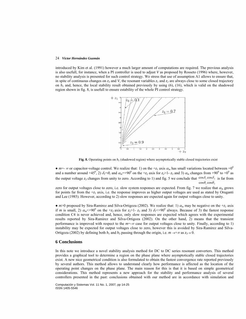
● m=-1 proposed by Rosseto (1996). We realize that: 1) on the +z1 axis αm has small variations located between approximately +450 and a number less than +900, 2) αm>+900 on the +z2 axis for z2>1-z3. Using C1 to analyse these cases we conclude that stability is expected for output voltages far from unity whereas stability is not ensured for output voltages close to unity. Further, using C4 we also conclude that the fastest convergence to the steady state, δ1=+900, will always occur for some output voltage far from unity. This agrees with the simulation and experimental results presented by Rosseto (1996). On the other hand, given some z2 and z3 we can use (6) to compute z1, i.e. these values represent an operating point on the phase plane where a closed trajectory exists. Now, we can use (12) to compute V. All of these values can be used in (16) to verify if 1

coscos

1

1 <θδ . Note that this condition is equivalen to

1coscoscoscos

31

31 <θθδδ in proposition 1, because closed trajectories are symmetric on the first and third quadrants. We can

repeat this procedure for several points on the phase plane to determine the region on the phase plane where operating points (on h1) corresponding to asymptotically stable closed trajectories exist. This region is represented by the shadowed region in fig. 8 where lines used to shadow such region represent the switching boundaries (6) for different values of z3. We stress that although this analysis might be also done using the eigenvalues based criterion




introduced by Kim et al. (1991) however a much larger amount of computations are required. The previous analysis is also usefull, for instance, when a PI controller is used to adjust V as proposed by Rosseto (1996) where, however, no stability analysis is presented for such control strategy. We stress that use of assumption A1 allows to ensure that, in spite of continuous changes on z3 and V, the resonant variables z1 and z2 are always close to some closed trajectory on h1 and, hence, the local stability result obtained previously by using (6), (16), which is valid on the shadowed region shown in fig. 8, is usefull to ensure estability of the whole PI control strategy.

Fig. 8. Operating points on h1 (shadowed region) where asymptotically stable closed trajectories exist

● m=- ∞ or capacitor-voltage control. We realize that: 1) on the +z1 axis αm has small variations located between +00 and a number around +450, 2) δ1=θ1 and αm=+900 on the +z2 axis for z2>1- z3 and 3) αm changes from +900 to +00 as the output voltage z3 changes from unity to zero. According to 1) and fig. 5 we conclude that

31

31

coscoscoscos

θθδδ is far from

zero for output voltages close to zero, i.e. slow system responses are expected. From fig. 7 we realize that αm grows for points far from the +z1 axis, i.e. the response improves as higher output voltages are used as stated by Oruganti and Lee (1985). However, according to 2) slow responses are expected again for output voltages close to unity.

● m>0 proposed by Sira-Ramirez and Silva-Ortigoza (2002). We realize that: 1) αm may be negative on the +z1 axis if m is small, 2) αm<+900 on the +z2 axis for z2>1- z3 and 3) δ1<+900 always. Because of 3) the fastest response condition C4 is never achieved and, hence, only slow responses are expected which agrees with the experimental results reported by Sira-Ramirez and Silva-Ortigoza (2002). On the other hand, 2) means that the transient performance is improved with respect to the m=-∞ case for output voltages close to unity. Finally, according to 1) instability may be expected for output voltages close to zero, however this is avoided by Sira-Ramirez and Silva-Ortigoza (2002) by defining both h1 and h3 passing through the origin, i.e. m →+∞ as z3→ 0.

6 Conclusions In this note we introduce a novel stability analysis method for DC to DC series resonant converters. This method provides a graphical tool to determine a region on the phase plane where asymptotically stable closed trajectories exist. A new nice geometrical condition is also formulated to obtain the fastest convergence rate reported previously by several authors. This method allows to understand clearly how performance is affected as the location of the operating point changes on the phase plane. The main reason for this is that it is based on simple geometrical considerations. This method represents a new approach for the stability and performance analysis of several controllers presented in the past: conclusions obtained with our method are in accordance with simulation and

ISSN 1405-5546


experimental results reported previously in the literature. We find that use of our method has several advantages when applied to several cases of study reported previously: 1) analysis is much simpler, 2) more insight into the problem is provided, 3) information is easily obtained about how performance is affected when the operating point changes. References

1. Kim M.G., D.S. Lee and M. J. Youn, “A new state feedback control of resonant converters”, IEEE Trans.

Industrial Electronics, Vol. 38, No. 3, 1991, pp. 173-179. 2. Kim M.G. and M. J. Youn, “An energy feedback control of series resonant converter”, IEEE Trans. Power

Electronics, Vol. 6, No. 3, 1991, pp. 338-345. 3. Oruganti R. and F. C. Lee, “Resonant power processors, Part I- State plane analysis”, IEEE Trans. Industry

Applications, Vol. AI-21, No. 6, 1985, pp. 1453-1460. 4. Oruganti R. and F. C. Lee, “Resonant power processors, Part II- Methods of control”, IEEE Trans. Industry

Applications, Vol. AI-21, No. 6, 1985, pp. 1461-1471. 5. Oruganti R., J.J. Yang and F. C. Lee, “Implementation of optimal trajectory control of series resonant

Converter”, IEEE Trans. Power Electronics, Vol. 3, No. 3, 1988, pp. 318-327. 6. Rossetto L., “A simple control technique for series resonant converters”, IEEE Trans. Power Electronics, Vol.

11, No. 4, 1996, pp. 554-560. 7. Sira-Ramirez H. and R. Silva-Ortigoza, “On the control of the resonant converter: a hybrid-flatness approach”,

in Proc. 15th International Symposium on Mathematical Theory of Networks and Systems, University of Notre Dame, South Bend, Indiana, August 12-16, 2002.

8. Stankovic A., D.J. Perreault and K. Sato, “Synthesis of Dissipative Nonlinear Controllers for Series Resonant DC/DC Converters”, IEEE Trans. on Power Electronics, Vol. 14, No. 4, 1999, pp. 673-682.

Victor Hernández Guzmán was born in Querétaro, Qro., México. He received the B. Sc., M. Sc. and PhD. degrees from Instituto Tecnológico de Querétaro (1988), Instituto Tecnológico de la Laguna (1991), and CINVESTAV (2003), respectively, all in Electrical Engineering. He is a professor at Universidad Autónoma de Querétaro where he teaches Classical Control, Linear Control Systems and Nonlinear Control Systems. His research interests include control in power electronics, robot control and control of underactuated mechanical systems. He likes to build mechanical prototypes to teach application of classical and modern control techniques.


Documents

Redalyc.A New Stability Analysis Method for DC to … · A New Stability Analysis Method for DC to DC Series Resonant Converters ... puramente geométricas en lugar de los eigenvalores