RECURSIVE SOLUTION METHODS FOR DYNAMIC LINEAR RATIONAL

Journal of Econometrics 41 (1989) 65-89. North-Holland

RECURSIVE SOLUTION METHODS FOR DYNAMIC LINEAR RATIONAL EXPECTATIONS MODELS*

Mark W. WATSON*

Norrhwestem lJniversi(~, Evanston, IL 60-708, USA and

National Bureau of Economy Reseurch

This paper develops recursive solution methods for linear rational expectations models. The underlying structural model is transformed into a state-space representation, which can then be used to solve the model and to form the Gaussian likelihood function. The recursive solution method has several advantages over other approaches. First, the set of solutions to the model are summarized by a set of parameters that appear in the state-space representation but are unspecified by the structural model. Next, the likelihood function is formed as a byproduct of the solution to the model. Finally, modifications in the likelihood function necessary to incorporate complications arising from temporal aggregation, dynamic errors-in-variables, etc. are straightforward.

1. Introduction

Models in which rational expectations of future values of variables are simultaneously determined with current values of these variables play an important role in economics and finance. Linear versions of these models have been used to model a wide variety of phenomena, but have posed some unique problems. The presence of endogenous future expectations together with current values makes these models more difficult to solve than standard linear models; moreover, the solutions are often nonunique.’ These models have also posed interesting econometric problems, which stem from the presence of unobserved expectations in the structural form of the model. Instrumental

*This paper has benefited from helpful comments and suggestions from seminar participants at Princeton. Rochester, Iowa, and Virginia. I owe particular thanks to Olivier Blanchard, Gary Chamberlain, Rob Engle, Charles Whiteman, and an anonymous referee. The financial support of the National Science Foundation is gratefully acknowledged.

‘A large number of solution procedures exist. See, for example, Blanchard and Kahn (19793, Whiteman (1983) Chow (1983) Gourieroux, Laffont, and Monfort (1982). and Braze. Gourier- oux, and Szafarz (1985).

0304-4076/89/$3.500 1989, Elsevier Science Publishers B.V. (North-Holland)

66 M. W. Wu~son, Recursive solution methods

variable estimators provide one solution to the problem.* Full information methods have also been developed and applied. [Examples are Sargent (1979) Hansen and Sargent (1980), and Blanchard (1983).]

Full information methods are generally difficult to implement. The usual practice is to find an analytic solution to the model which produces a reduced form relating current and lagged values of the endogenous variables to current and lagged values of the exogenous variables, some disturbances, and the parameters of the model. This reduced form usually implies that the data can be represented as a vector ARMA process with complicated constraints connecting the ARMA coefficients. This constrained ARMA model can then be estimated by nonlinear maximum likelihood methods.

In this paper I propose an alternative procedure for solving and estimating dynamic linear rational expectations models. The method relies on the state-space representation of the model. The state-space approach to the formulation and estimation of dynamic linear rational expectations models has several advantages over other approaches. First, the constraints that the model places on the data are transparent. The complete set of solutions to the model is conveniently summarized by a set of parameters that is not determined in the structural model, nor by the process generating the exogenous variables. Next, the model is easily solved recursively by the Kalman filter; an algebraic solution to the model is unnecessary. As byproducts of the recursive solution procedure the Kalman filter produces the innovations and innovation vari- ances of the observed data. These are the basic building blocks of the Gaussian likelihood function. Finally, and of particular importance in applied work, modifications in the empirical model that are necessary because of data limitations are easily incorporated. Modifications in the likelihood function necessary to incorporate complications arising from missing observations, temporal aggregation, interpolation, and dynamic errors-in-variables are straightforward. [The necessary modifications are analogous to those discussed in Harvey, McKenzie, Blake, and Desai (1981) Harvey and Pierse (1984), and Hausman and Watson (1985).]

This paper begins, in section 2, with a very simple model with one endogenous variable, one future expectation, and one exogenous variable. Most of the key features of the state-space representation of dynamic linear rational expectations models can be presented using this simple example. In section 3 we present the generalization of this model with more exogenous variables, longer future expectations, and lags of the endogenous variable, etc. In section 4 we discuss properties of the estimated parameters obtained by maximizing a Gaussian likelihood function, and show the importance of imposing stationar-

‘The original IV estimator was suggested by McCallum (1976). A systematic discussion of IV estimators in dynamic linear rational expectations models can be found in Hansen and Sargent (1982).

M. W. Watson, Recursive solution methods 67

ity on the solution of the model. An empirical study investigating the relationship between stock prices and dividends is presented in section 5, and some concluding remarks are offered in section 6.

2. A simple example

Many of the important characteristics of the recursive solution of linear dynamic rational expectations models can be illustrated with a simple example. In this section we analyze such a model in detail, and in the next section we discuss a generalization. The model that we consider is

Y t+ 1/r = PY, + x, 7 t= 1,2,..., (2.1)

x, = +x,- 1 + e,f, t = 1,2,..., (2.2)

= x0. (2.3)

where Ic$/ and iid and variance Eq. (2.1) is the relation between the expected value of y,+,

at time t, by ~!+i,~, the actual of y time t, by y,. and an x,. Eq. (2.2) is equation of for x,, and (2.3) the initial condition for x,. We the expectation

i,, formed rationally:

~r+l/r = E(Y~+,P,)~ (2.4)

where 9, is the set of information available at time t. Throughout this paper

we use I~,,-, to denote E( z,l tit_,), where the information set L?_, will be clear from the context, We will assume that (x,, y,) E 9, and L?_i c fiC for f= 1,2,... .

Many models fit into this framework. Eq. (2.1) can be viewed as a (re- arranged) money demand equation in which y and x are the logarithms of the price level and the quantity of money, respectively. In this interpretation eq. (2.1) describes the demand for real balances as a function of expected price inflation. Alternatively, y, can be viewed as the price of an asset, x, as the value of services realized for the ownership of the asset, and (2.1) is a standard arbitrage equation.

The recursive solution for the model relies on a reduced form that expresses the variables at time t in terms of predetermined variables and innovations. This reduced form leads directly to the state-space representation of the model. It describes the evolution of all variables of interest, including the

68 M. W. Watson, Recursive solution methods

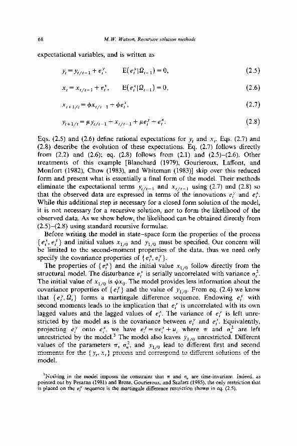
expectational variables, and is written as

Yt = Y,/,- 1+ e:, E(ePlfi,-,) = 0, (2.5)

x, = x,/,-~ + ef, E(eFlfL,) = 0, (2.6)

x,+ l/1 = CPX r/r-1 + +e:, (2.7)

Y r+l/t = PY~/,-~ + x,/,-~ + cLeY + C. (2.8)

Eqs. (2.5) and (2.6) define rational expectations for y, and x,. Eqs. (2.7) and (2.8) describe the evolution of these expectations. Eq. (2.7) follows directly from (2.2) and (2.6); eq. (2.8) follows from (2.1) and (2.5)-(2.6). Other treatments of this example [Blanchard (1979) Gourieroux, Laffont, and Monfort (1982) Chow (1983) and Whiteman (1983)] skip over this reduced form and present what is essentially a final form of the model. Their methods eliminate the expectational terms ~,,~_r and x,,,_~ using (2.7) and (2.8) so that the observed data are expressed in terms of the innovations e{ and e:. While this additional step is necessary for a closed form solution of the model, it is not necessary for a recursive solution, nor to form the likelihood of the observed data. As we show below, the likelihood can be obtained directly from (2.5)-(2.8) using standard recursive formulae.

Before writing the model in state-space form the properties of the process {e;, e/‘} and initial values X~,~ and yI,O must be specified. Our concern will be limited to the second-moment properties of the data, thus we need only specify the covariance properties of { e:, ey }.

The properties of {e,“} and the initial value xl/0 follow directly from the structural model. The disturbance ef is serially uncorrelated with variance u,‘.

. . . The mitral value of xl/0 is +x,. The model provides less information about the covariance properties of {e,‘} and the value of y,,,. From eq. (2.4) we know that {e/‘, 52,) forms a martingale difference sequence. Endowing e: with second moments leads to the implication that e/’ is uncorrelated with its own lagged values and the lagged values of e:. The variance of ey is left unrestricted by the model as is the covariance between ey and e:. Equivalently, projecting e,Y onto e:, we have ef = rre: + u, where r and 0,’ are left unrestricted by the model.3 The model also leaves ~t,~ unrestricted. Different values of the parameters r, u,‘, and yI,O lead to different first and second moments for the { y,, xt} process and correspond to different solutions of the model.

3Nothing in the model imposes the constraint that B and ou are time-invariant. Indeed, as pointed out by Pesaran (1981) and Broze, Gourieroux, and Szafa (1985), the only restriction that is placed on the ey sequence is the martingale difference restriction shown in eq. (2.5).

A!. W. Watson, Recursive solution methods 69

These three parameters completely characterize the set of solutions to (2.1)-(2.3) which have a time-invariant parameterization and describe the first two moments of { y,, x,}. It is instructive to interpret these parameters in terms of other solutions that have appeared in the literature. The disturbance u, represents a shock to the expectations of future y,‘s that is uncorrelated with the fundamental driving variable x,. It represents a ‘stochastic bubble’, discussed in Blanchard and Watson (1982), Grossman and Diba (1983) West (1986), and elsewhere. The parameter 2 a, indexes the relative importance of this stochastic bubble. The coefficient 7~ transmits new information about the current values of x to the expectations of future values of y. It determines whether the process is ‘forward looking’ or ‘backward looking’ or some combination of both [see Blanchard (1979)]. Finally, the coefficient y,,, represents the initial condition for the expectations process. It reflects the initial information about the influence of x on future y and the influence of any ‘deterministic bubbles’ on future y. [See Flood and Garber (1980).]

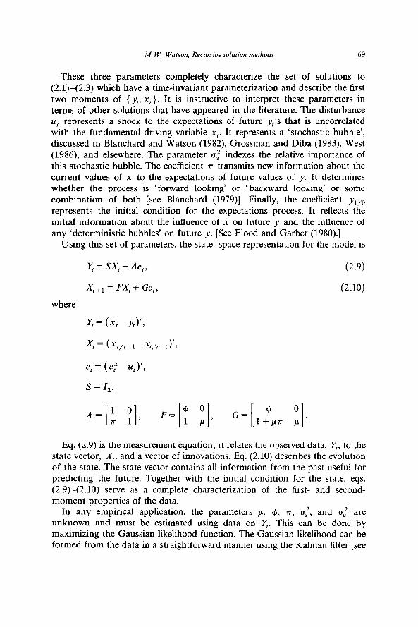
Using this set of parameters, the state-space representation for the model is

q = SX, + Ae,,

x t+l=FXt+Ge,,

(2.9)

(2.10)

where

r, = (x, YJ’?

x, = (X,/,-l Yt,,-A',

e, = (ef uf)‘,

S=I,,

Eq. (2.9) is the measurement equation; it relates the observed data, q, to the state vector, X,, and a vector of innovations. Eq. (2.10) describes the evolution of the state. The state vector contains all information from the past useful for predicting the future. Together with the initial condition for the state, eqs. (2.9)-(2.10) serve as a complete characterization of the first- and second- moment properties of the data.

In any empirical application, the parameters p, c$, r, o,‘, and u,’ are unknown and must be estimated using data on y. This can be done by maximizing the Gaussian likelihood function. The Gaussian likelihood can be formed from the data in a straightforward manner using the Kalman filter [see

70 M. W. Watson. Recursive solution methods

Schweppe (1965) or Harvey (1982)]. The properties of estimators formed by maximizing this function are the subject of section 4.

In many specific applications of the model, the parameter p is restricted a priori to be larger than one. For instance, in the stock price/dividend interpretation of the model, the parameter p = (1 + r) where r is the interest rate. Since p is an eigenvalue of the state transition matrix, F, this implies that a linear combination of the expectations x,/,-i, ~~,~_t is exploding. But with I+( < 1, x, is stationary, so that any explosive behavior must be occurring in yI. For a variety of reasons it may be reasonable to rule out this type behavior a priori. For instance, one might insist on a solution to the model in which stationary inputs (x) lead to stationary outputs (y). This can usually be accomplished by choosing a parameterization which annihilates the linear combination of the elements of the state vector corresponding to the explosive root. In this example the explosive linear combination is given by ~!+i,~ =

Yt+l/r+Xr+l/l I* ( - c#B)-‘. Substituting from (2.7) and (2.8) we have

W f-cl/l = PY/,-1-t dce: + 4) (2.11)

where c = 7~ + (II - $I-‘. When p > 1, the expectations of future y will explode (almost surely) as r increases unless w,+i,, = 0 for all t. This explosive behavior can be ruled out if and only if

Y/O = 0 - .Y,/o= -xl/oh - (P>-‘> (2.12)

c=o =a n= (+-p)-‘, (2.13)

2.4, = 0, t = 1,2,... j u;=o. (2.14)

This nonexplosiveness condition imposes three constraints on the model when p > 1. These three constraints, given in (2.12)-(2.13) exactly determine the three parameters y,,,, 7~, and a, that characterize the set of solutions to the model (2.1)-(2.3). The uniqueness of the solution in this case has been pointed out in many places. It is implied by Proposition 1 of Blanchard and Kahn (1980), Lemma 1 of Whiteman (1983) and Theorem 5.5 of Braze, Gourieroux, and Szafarz (1985).

In this simple model, condition (2.14) implies that the bivariate (x,, y,) process is singular, and thus is a condition that would be rejected in any empirical setting. However, this singularity is an artifact of the very simple structure underlying the example used in this section. In the next section a more general structure is introduced and this singularity disappears. Stationar- ity in these more general structures does require knife-edge parametric constraints analogous to (2.12) and (2.13).

M. W. Watson, Recursive solurion methods 71

3. A generalization

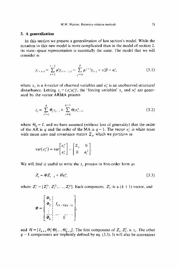
In this section we present a generalization of last section’s model. While the notation in this new model is more complicated than in the model of section 2, its state-space representation is essentially the same. The model that we will consider is

r-1 P

Y,+r/t = c P’Y,+,-,,t + c PY,_’ + XiP + 4, (3.1) r=l J=o

where x, is a k-vector of observed variables and U: is an unobserved structural disturbance. Letting z, = (x;u;)‘, the ‘forcing variables’ x, and us are generated by the vector ARMA process

4 q-1 2, = C @,Z,_, + C @ief-,,

r=l r=O

(3.2)

where 0, = I, and we have assumed (without loss of generality) that the order of the AR is q and the order of the MA is q - 1. The vector e: is white noise with mean zero and covariance matrix ,X,, which we partition as

We will find it useful to write the z, process in first-order form as

2, = @Z,_l + He:, (3.3)

where Z,’ = [Z:‘, Zf’, . . , Zp’]. Each component, Z:, is a (k + 1) vector, and @ 1 I @2 I &+l)(q-1)

@= .I I I3 . I

_~-;__---_--_

Q, 41 0

and H = [Ik+, 0; 0;. . . t3_ J’. The first component of Z,, Z:, is z,. The other q - 1 components are implicitly defined by eq. (3.3). It will also be convenient

12 M. W. Watson, Recursive solutron methods

to stack the endogenous variables into a vector

yp= [J&l,,, Yt+r-2/,,*-., Yt+1/r, Yt, Yf-l?..., Yf-,I’.

Eq. (3.1) can then be written as

pt p2 ... I CL*+’

P= 0

I---------Y-

I r+p-1 I :

0

(3.4)

[

D 0 6=

IX(q-l)(k-cl)

0 (r+p-l)x(k+l) 0 (r+p-l)X(q-l)(k+l) I3 where p is the 1 (k 1) p= [/I’ll and Okx, is a k Xj matrix of zeros. We assume that the initial condition for Z, is

z, = zo. (3.5)

Eqs. (3.3)-(3.5) are the multivariate analogues of (2.1)-(2.3). The reduced form of (3.3)-(3.5) is

yp =yt’/,-1 + q> E[ $‘I&1] = 0, (3.6)

z, = .2&l + E:, E[~:lQt-l] = 0, (3.7)

Z t+1/, = @-q-l + Q&:7 (3.8)

Y t& = PY;,-l+ Sq-1 + l-4 + 6&f> (3.9)

where ET = He: from (3.3). Since the vector yp contains lagged values of y,, which are known at time t - 1, many of the elements of E;V are zero. We will write E/ as

Ey= [E:-l,t,E;-2,t )..., Eg,, 0,o ,..., 01,

M. W. Watson. Recursive solution methods 73

where

&,‘l , = y,+j/,-Y,+j/t-1 for j = O,l,..., r- 1.

This reduced form can be used to discuss the set of solutions to the model (3.3)-(3.5). We restrict ourselves to solutions with time-invariant parameterizations which describe the first and second moments of the {x,. )I~} process. Eqs. (3.7) and (3.8) together with E:, completely characterize the {x,} process. Eqs. (3.6) and (3.9) describe the generation of y,. The y, data are driven by the exogenous variables Z, plus the innovations ~1,. These E,‘, innovations are martingale difference sequences with respect to fir_,. Together with the set of

. . initial condttrons given by J&, these sequences determine the set of solutions to the model [see Broze, Gourieroux, and Szafarz (1985)]. Since our concern is with the first and second moments of (x,, y,) we need (i) the initial conditions yf,a and (ii) the covariance properties of E:. These are left unspecified by the (3.3)-(3.5) so that the solution to the model characterized by (3.6)-(3.9) is not unique. The set of solutions can be parameterized by the r + p initial conditions JJ;,,, the r(r + 1)/2 parameters in the covariance matrix of ET, and the r(k + 1) covariances between E: and ~j’. Alternatively, if we let e: =

[E;Y_ 1, I, c;._z, *, . . . , E&I’ denote the nonzero elements of ET and project e: onto

e ,Z, we have

ey = fief + 24 f, (3.10)

where U, and e: are uncorrelated and var(u,) = _IYU. (The reason for the - over II will soon be clear.) The set of solutions_is characterized by the (r + p) + r( k + 1) + r( r + 1)/2 parameters in Y:,~, II, and 2,.

The model (3.6)-(3.9) can now be written in state-space form. One state-space representation is

r, = SX, + &, (3.11)

X r+l = FX,+ Get, (3.12)

where q is the k + 1 vector [x,! JJ,], X, is the n x 1 vector [ Z;,t_ I r:;l_ 1]’ [where n = (k + 1)q + r +p], S is a (k + 1) x n selection matrix which selects X r,+1 and A,,-~ from the state vector. The innovation vector E; = [e:’ ~~1,

and 2’ = [A;’ ai!, where AI is k X (k + 1 + r) and 2, is 1 X (k + 1 + r).

These blocks are A, = [I, Okxcr+lj] and A, = [ii, l,], where ii, is the r th row of fi and I, is an r x 1 row vector with O’s in every entry except the last, which is equal to 1. Thus the innovation in x, is jtat = E: and the innovation in y, is &Y 0 I which is written as E{ f = ji,$ + lrut from (3.10).

74 M. W. Watson, Recurswe solution methods

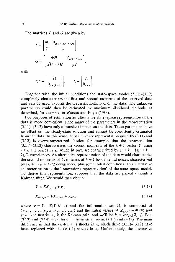
The matrices F and G are given by

with

Together with the initial conditions the state-space model (3.11)-(3.12) completely characterizes the first and second moments of the observed data and can be used to form the Gaussian likelihood of the data. The unknown parameters could then be estimated by maximum likelihood methods, as described, for example, in Watson and Engle (1983).

For purposes of estimation an alternative state-space representation of the data is more convenient, since many of the parameters in the representation (3.11)-(3.12) have only a transient impact on the data. These parameters have no effect on the steady-state solution and cannot be consistently estimated from the data. In this sense the state-space representation given by (3.11) and (3.12) is overparameterized. Notice, for example, that the representation (3.11)-(3.12) characterizes the second moments of the k + 1 vector Y using r + k + 1 noises in E,, which in turn are characterized by (r + k + l)( r + k + 2)/2 covariances. An alternative representation of the data would characterize the second moments of Y in terms of k + 1 fundamental noises, characterized by (k + l)(k + 2)/2 covariances, plus some initial conditions. This alternative characterization is the ‘innovations representation’ of the state-space model. To derive this representation, suppose that the data are passed through a Kalman filter. We would then obtain

y = sx,,,-, + vr, (3.13)

X r+l/r=W,,-1 +K,v,, (3.14)

where v, = Y, - E( Y,Is2,_,) and the information set 9, is composed of

(Y,, _Y-l>... ,Y1.Xr,X,-l~..-, xl) and the initial values of Z,,, (= @ZO) and

yf,,. The matrix K, is the Kalman gain, and we’ll let h, = var( ~~19,~ 1). Eqs. (3.13) and (3.14) have the same basic structure as (3.11) and (3.12). The main difference is that the (k + 1 + r) shocks in E, which drive (3.11)-(3.12) have been replaced with the (k + 1) shocks in vl. Unfortunately, the alternative


representation is not time-invariant since both h, and K, will, in general, depend on t. However, for our particular model it is possible to show that both h, and K, converge to steady state values and therefore eqs. (3.13) and (3.14) can serve as a convenient parsimonious steady-state characterization of the second-moment properties of the data. This result is stated formally in:

Theorem I. For the model given by (3.13)-(3.14) with given initial conditions

we have

6) lim h,=h, 1-00

(ii) lim K, = K, /+CC

(iii) h can be written as AQA’,

(iv> K can be written as GA ~‘,

where the parameterizations of h and K are chosen to mimic the structure of (3.11) and (3.12). In particular,

G = [ pn%f] with no= [ opx:+J, II is an r X (k + 1) matrix, A’ = [A; A;], where A, is k X (k + 1) and A, is

1 X (k + 1). These blocks are A, = [ Ik 0] and A, = ?r,, where V~ is the rth row of the matrix II appearing in G. Finally, Q is a (k + 1) X (k + 1) matrix:

Proof. See appendix.

The intuition underlying the theorem is straightforward. The representation of the model given in (3.11) and (3.12) describes the k + 1 elements in Y, in terms of the k + 1 + r elements of the noise vector Ed. The multivariate Wold representation theorem suggests that we should be able to characterize the second-moment properties of the k + 1 elements in Y, using a noise vector containing just k + 1 elements, and this is just what the innovations representation of the model does. The specific initial conditions assumed in (3.11) and (3.12) lead to some transient heteroskedasticity in the innovations4

41nitial conditions in time series models often leads to transient heteroskedasticity in the innovation series. ARMA models provide one example.


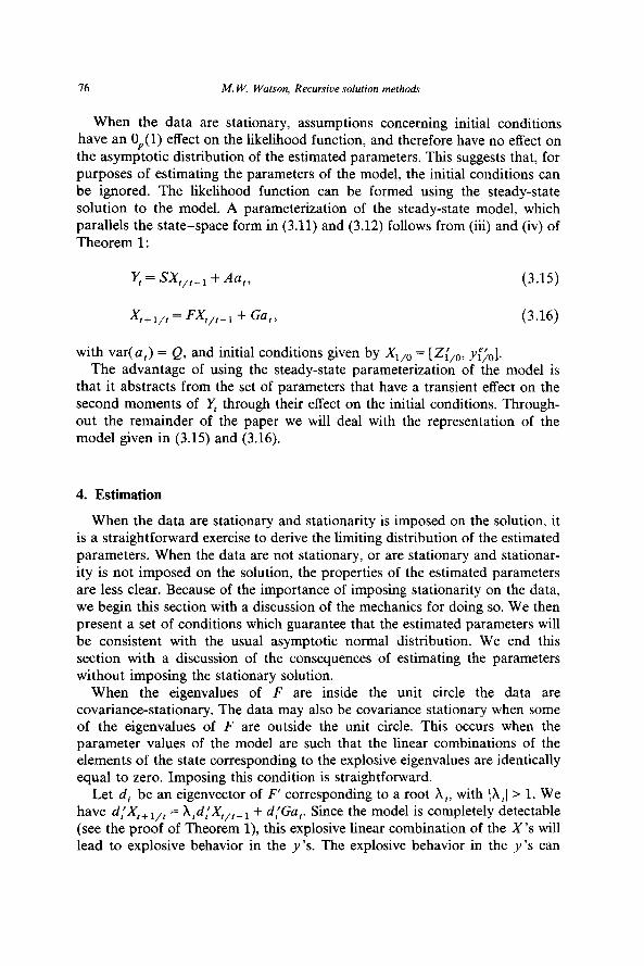
When the data are stationary, assumptions concerning initial conditions have an O,,(l) effect on the likelihood function, and therefore have no effect on the asymptotic distribution of the estimated parameters. This suggests that, for purposes of estimating the parameters of the model, the initial conditions can be ignored. The likelihood function can be formed using the steady-state solution to the model. A parameterization of the steady-state model, which parallels the state-space form in (3.11) and (3.12) follows from (iii) and (iv) of

Theorem 1:

r, = sx,,,_, + Aa,,

X t+ 1/r = FX1,,_, + Ga,,

(3.15)

(3.16)

with var( a,) = Q, and initial conditions given by X1,0 = [Z;,,, y&l. The advantage of using the steady-state parameterization of the model is

that it abstracts from the set of parameters that have a transient effect on the second moments of Y, through their effect on the initial conditions. Through- out the remainder of the paper we will deal with the representation of the model given in (3.15) and (3.16).

4. Estimation

When the data are stationary and stationarity is imposed on the solution, it is a straightforward exercise to derive the limiting distribution of the estimated parameters. When the data are not stationary, or are stationary and stationarity is not imposed on the solution, the properties of the estimated parameters are less clear. Because of the importance of imposing stationarity on the data, we begin this section with a discussion of the mechanics for doing so. We then present a set of conditions which guarantee that the estimated parameters will be consistent with the usual asymptotic normal distribution. We end this section with a discussion of the consequences ‘of estimating the parameters without imposing the stationary solution.

When the eigenvalues of F are inside the unit circle the data are covariance-stationary. The data may also be covariance stationary when some of the eigenvalues of F are outside the unit circle. This occurs when the parameter values of the model are such that the linear combinations of the elements of the state corresponding to the explosive eigenvalues are identically equal to zero. Imposing this condition is straightforward.

Let dj be an eigenvector of F’ corresponding to a root Xi, with ]Xi] > 1. We have d;X,, l,r = Xid/Xt,,_1 + d[Ga,. Since the model is completely detectable (see the proof of Theorem l), this explosive linear combination of the X’s will lead to explosive behavior in the y ‘s. The explosive behavior in the y’s can


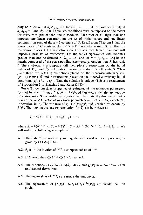
only be ruled out if d/X,+ i,, = 0 for t = 1,2,. . . . But this will occur only if d!X,,, = 0 and d,‘G = 0. These two conditions must be imposed on the model

for every root greater than one in modulus. Each root of F larger than one imposes one linear constraint on the set of initial values and one linear constraint on each of the k + 1 columns of G. Recall from Theorem 1 that the lower block of G contains the r X (k + 1) parameter matrix 17, so that the restriction places k + 1 restrictions on II. Each root larger than one will impose a new set of restrictions. Let the set of eigenvalues with modulus greater than one be denoted Xi, h,, . . . , hj and let R = [cl, c2,. . . , cj] be the matrix composed of the corresponding eigenvectors. Assume that R has rank j. The stationarity assumption will then place J restrictions on the initial values of X1,0 and j( k + 1) restrictions on the matrix of coefficients II. When

j = r there are r( k + 1) restrictions placed on the otherwise arbitrary r x

(k + 1) matrix II and r restrictions placed on the otherwise arbitrary initial

conditions y{, y[, . . . , v,‘_~. Thus the solution is unique. [This is a restatement

of Proposition 1 in Blanchard and Kahn (1980).]

We will now consider properties of estimates of the unknown parameters formed by maximizing a Gaussian likelihood function under the assumption of stationarity. Some additional notation will facilitate the discussion. Let 0 denote the m x 1 vector of unknown parameters and let vI = Au, denote the innovation in y. The variance of v, is A(S)Q(ti)A(S)‘, which we denote by h (0). The moving average representation for y can be written as

r, = c,a, + c,a,_, + c*a,_, + . . . 3

where Z, = h(f3)-‘/2~,, C, = h(B) ‘12, Ci=SF’-‘GAp’h’/2 for i= 1,2,... . We will make the following assumptions:

A.l. The data q are stationary and ergodic with a state-space representation given by (3.15)-(3.16).

A.2. 9, is in the interior of We, a compact subset of R”.

A.3. If 8’ # 0,, then C,(e’) # C,(S,) for some i.

A.4. The functions F(e), G(B), S(e), A(B), and Q(e) have continuous first and second derivatives.

A.5. The eigenvalues of F(fl,) are inside the unit circle.

A.6. The eigenvalues of [ F(8,) - G( Bo)A(Bo)-lS(S(Bo)] are inside the unit circle.

78

A.7. Let

(i> (ii) (iii)

M. W. Watson, Recursive solution methods

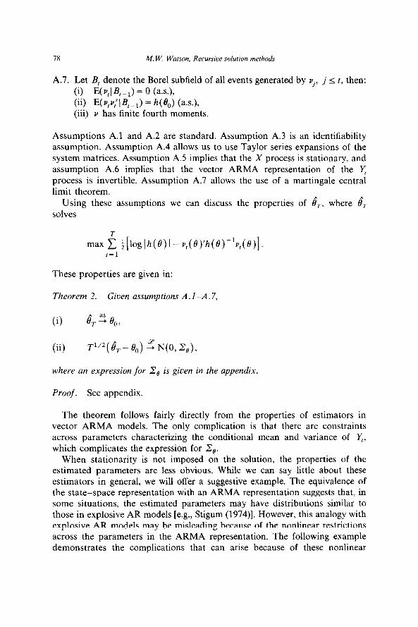
B, denote the Bore1 subfield of all events generated by v,, j I t, then:

E(v,jB,_,) = 0 (as.),

E(v,q’l%,) = h(4) (a.s.), v has finite fourth moments.

Assumptions A.1 and A.2 are standard. Assumption A.3 is an identifiability assumption. Assumption A.4 allows us to use Taylor series expansions of the system matrices. Assumption A.5 implies that the X process is stationary, and assumption A.6 implies that the vector ARMA representation of the Y, process is invertible. Assumption A.7 allows the use of a martingale central limit theorem.

Using these assumptions we can discuss the properties of ir., where $T solves

maxi ~[log]h(B)(-v,(B)‘h(8))1v,(~)]. r=l

These properties are given in:

Theorem 2. Given assumptions A.1 -A.7,

(ii) T’/2( e,- 8,) ,” N(0, Z,),

where an expression for I0 is given in the appendix.

Proof. See appendix.

The theorem follows fairly directly from the properties of estimators in vector ARMA models. The only complication is that there are constraints across parameters characterizing the conditional mean and variance of Y,, which complicates the expression for Ze.

When stationarity is not imposed on the solution, the properties of the estimated parameters are less obvious. While we can say little about these estimators in general, we will offer a suggestive example. The equivalence of the state-space representation with an ARMA representation suggests that, in some situations, the estimated parameters may have distributions similar to those in explosive AR models [e.g., Stigum (1974)]. However, this analogy with explosive AR models may be misleading because of the nonlinear restrictions across the parameters in the ARMA representation. The following example demonstrates the complications that can arise because of these nonlinear

M. W. Watson, Recursive solutron methods 79

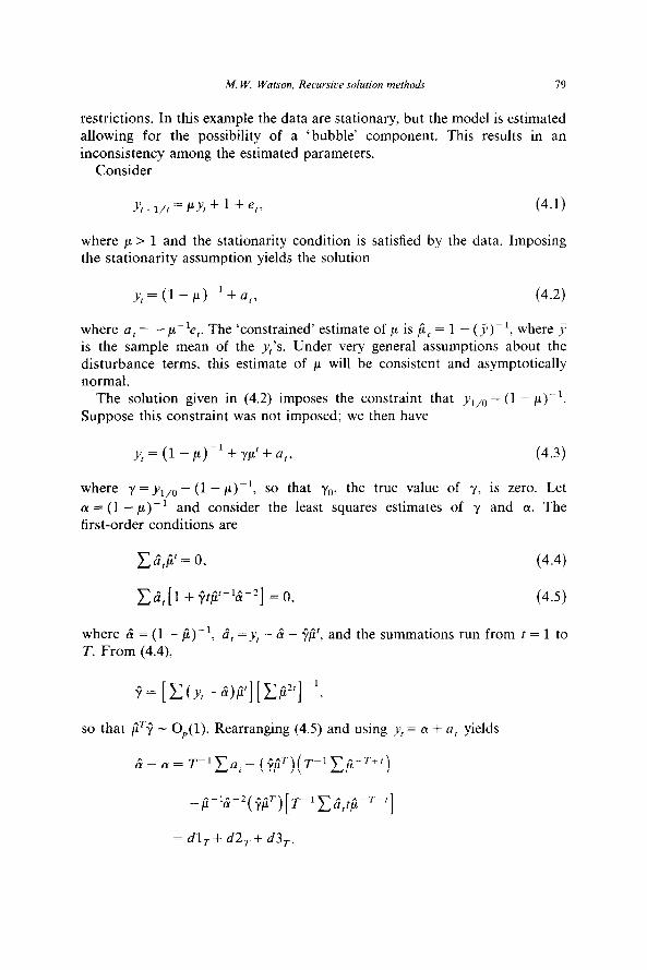
restrictions. In this example the data are stationary, but the model is estimated allowing for the possibility of a ‘bubble’ component. This results in an inconsistency among the estimated parameters.

Consider

Y,+ 1/r = PLY, + 1 + e,, (4.1)

where y. > 1 and the stationarity condition is satisfied by the data. Imposing the stationarity assumption yields the solution

y, = (1 - p) -l+ a,, (4.2)

where a, = -p-‘e,. The ‘constrained’ estimate of p is PC = 1 - (j))‘, where ,t; is the sample mean of the y,‘s. Under very general assumptions about the disturbance terms, this estimate of p will be consistent and asymptotically normal.

The solution given in (4.2) imposes the constraint that ~i,~ = (1 - p))‘. Suppose this constraint was not imposed; we then have

y,=(l-#+$+a,, (4.3)

where y = y,,, - (1 - p))l, so that yO, the true value of y, is zero. Let

(Y = (1 - I*)-~ and consider the least squares estimates of y and (Y. The first-order conditions are

c l?,fi’ = 0, (4.4)

&?,[l + ftfi’-‘&-*I = 0, (4.5)

where d = (1 - fi)-‘, 8, =_y, - 6 - +$I, and the summations run from r = 1 to T. From (4.4),

9= [c(Yt-w][D2t]-1>

so that CT? - O,(l). Rearranging (4.5) and using y, = cy + a, yields

= dl,+ d2,+ d3,.


The first term, dl,, represents the difference between & and LY when the stationarity constraint is imposed. The second term will vanish in probability when fi > 1. The final term, d3,, will not vanish in probability; each of the terms fi-W’, (j$r), [TP’Ca^,tb-T+f] is O,(l) but none are o,(l). Thus the discrepancy & - (Y will be bounded in probability but will not converge to zero. The cause of the inconsistency in & can be seen by rewriting the first-order condition (4.5) as

(4.6)

where c, = &i-2$T-’ - O,(l). Eq. (4.6) shows that & is found by setting a weighted sum of the residuals equal to zero. Since the weights are OP(tjFT), nearly all of the weight is placed on the last few observations; in essence, ai is determined by a small sample, even asymptotically. Note, however, that even though (Y and thus p are not estimated consistently, f can be expected to be very close to zero when 1; > 1, since fi’? is bounded in probability.

5. Stock prices and dividends

One interpretation of the model presented in section 2 is an arbitrage relationship between the price of a portfolio of stocks and the dividends paid on the portfolio. Letting P, denote the portfolio price, d, denote the value of dividend accruing to portfolio, and p denote the (constant) real gross rate of interest, this arbitrage relationship can be written as

E(~,+,lfi,) =P(P,-4). (5.1)

This follows from the assumption of risk neutrality on the part of investors who share a common set of information fi,. One solution to eq. (5.1) is the ‘forward looking’ or ‘fundamental’ solution given by

PI = E ~-iE@,+,l~t)~ i=O

(5.2)

This expresses p, as the discounted present value of expected future dividends.’ In this section we carry out a test of (5.1) and the particular solution given in (5.2) using the methods developed in the previous sections.

‘The relationship given in (5.2) has been the subject of a large number of empirical tests. The recent literature includes Shiller (1981), Blanchard and Watson (1982), Engle and Watson (1985). Campbell and Shiller (1986), and West (1986).

M. W. Wutson. Recursive solution methods 81

To begin, an equation of motion for d, is necessary. We assume that d, is generated by

d r+l=x$+E,+l, (5.3)

where x, is a set of variables known to the investor at time t and <,+, is an innovation which is uncorrelated with all information in 0,. Our empirical analysis will use data on price and dividends only, so that the implications of (5.1)-(5.3) for the joint process describing pt and d, must be derived. We will assume that dividends follow an integrated process and that Ad, is covari- ante-stationary. As Engle and Watson (1985) and Campbell and Shiller (1986) point out, the relationship given in (5.2) implies that p, is also integrated and that p, and d, are cointegrated. The series pt - ld,, with 5 = p(p - 1)-l, is covariance-stationary.

To derive the bivariate process describing p, and d,, project x, onto current and lagged values of d, and p, which yields

(5.4)

where @(II), y(B), o(B), and p(B) are one-sided polynomials in the back- shift operator B. The error ef+r is the innovation in d,,, that arises from an information set consisting of past dividends and prices. The scale of ~f+r is identified using the normalization o0 = 1. Following the notation introduced in the previous sections we let EP denote the innovation in pt formed from this restricted information set. Projecting E/’ onto E: yields

where U, and E,” are uncorrelated white noise proccesses. The error correction term ( pr - {d,) may appear in (5.4) because of the cointegration implied by (5.2) [see Engle and Granger (1987)].

In our empirical model we assume that G(B) is a polynomial of order two, w(B) is a polynomial of order one, y(B) = y, and p(B) = p. This implies

d r+l/t = (1 + +I- 4d,,,-l + h - +l)d,-1 - G-2

+ (Y + dP,,r-1 - YPr-1 + Q,d+ X2%,

where

(5.5)

A,= -W1+(l+~,-~,~)+~(y+al),

h2=p+y+a1.


The model can then be written in state-space form (3.16) with

X I+ 1/t =

r

d 1+1/r

d, d r-1

Pt+1/t

Pt

G=

I 1 + @I - 41 $2 - $1

1 0

F==

0 1 -P 0

0 0

Xl x2

1 0

0 0 9

!-G-l) I* ll 1

given in (3.15) and

-+2 Y+% -Y

0

0 0 0 0 0. 0 P 0

0 1 0 1

The parameter p is the gross rate of interest so that p > 1, and for reasonable values of the parameters +~i, +)2, (pi, 5, and y, the matrix F will have one eigenvalue with modulus greater than 1. The forward looking solution given in (5.2) is chosen by annihilating the linear combination of the elements of the state vector associated with this explosive root. This imposes one constraint on the vector of initial conditions Xi,0 and one constraint on each column of G.

The data that are used in the analysis are the Dow Jones annual data used in Shiller (1981). The sample period is 1928-1978. We let 1930 correspond to t = 1 and use the data from 1928 and 1929 to serve as initial conditions d,, d and P_~. The initial values of d,,, and pl,o were estimated imposing the co&traint mentioned in the last paragraph.

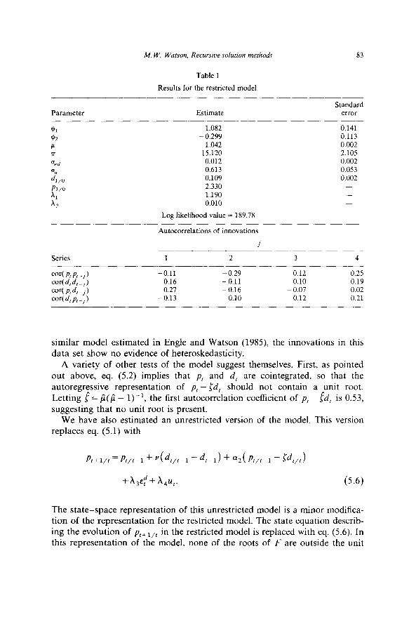
Results are given in table 1. Choosing the forward looking stable solution makes the parameters A, and A, implicit functions of T and p because of the constraints imposed on the columns of G. In addition, the initial condition pl,o is an implicit function of d,,,, d,, d_,, and po, because of the constraint imposed on Xr,a. The two coefficients y and (pi were very small and insignificant in every model estimated. The results shown in table 1 constrain these coefficients to equal zero. In the bottom panel of the table we show the autocorrelations of the fitted innovations from the model. These should be vector white noise, and the results suggest that this is not too far from the truth. There are two slightly troublesome values: cor( ~~p,_~) = -0.29 and cor( ptd,_ 1) = 0.27, but the sample size is only 49. Unlike the results for a


Table 1

Results for the restricted model.

Estimate

1.082 - 0.299

1.042 15.120

0.012 0.613 0.109 2.330 1.190 0.010

Log likelihood value = 189.78

Standard error

0.141 0.113 0.002 2.105 0.002 0.053 0.002

_

Autocorrelations of innovations

_i

Series __- cor( P, P, 1 -, cor(d,d,-,I cor( P, d, 1 -, cor( d, pt 1 -,

1 2 3 4

-0.11 -0.29 0.12 0.25 0.16 -0.11 0.10 0.19 0.27 -0.16 - 0.07 0.02

-0.13 0.10 0.12 0.21

similar model estimated in Engle and Watson (1985) the innovations in this data set show no evidence of heteroskedasticity.

A variety of other tests of the model suggest themselves. First, as pointed out above, eq. (5.2) implies that pt and d, are cointegrated, so that the autoregressive representation of pt - Id, should not contain a unit root. Letting f = fi(fi - l))‘, the first autocorrelation coefficient of pr - ltid, is 0.53, suggesting that no unit root is present.

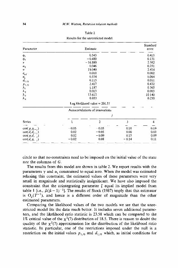
We have also estimated an unrestricted version of the model. This version replaces eq. (5.1) with

Pt+ l/r =pt/t-1+ “(4/,-l -4-J + %(P,,t-1 - W/t)

+X3&;+ xp,. (5.6)

The state-space representation of this unrestricted model is a minor modifica- tion of the representation for the restricted model. The state equation describing the evolution of P~+~,,~ in the restricted model is replaced with eq. (5.6). In this representation of the model, none of the roots of F are outside the unit


Table 2

Results for the unrestricted model.

Parameter Estimate Standard

error

0.543 0.413 - 0.480 0.131

- 16.880 2.582 - 0.046 0.251 19.040 2.414 0.010 0.002 0.574 0.064 0.115 0.011 2.411 0.432 1.187 0.365 0.013 0.003

13.612 10.140 0.953 0.230

Log likelihood value = 201.57

Autocorrelations of innovations

Series

cor(p,k,) cor( d, d, ) -, cNp,d,-,I cor( d, P, -, )

1 2 3 4

- 0.05 - 0.05 0.18 0.19 - 0.02 0.05 0.00 0.03

0.02 - 0.09 0.15 0.09 - 0.02 0.08 -0.14 0.11

circle so that no constraints need to be imposed on the initial value of the state nor the columns of G.

The results from this model are shown in table 2. We report results with the parameters y and (pi constrained to equal zero. When the model was estimated relaxing this constraint, the estimated values of these parameters were very small in magnitude and statistically insignificant. We have also imposed the constraint that the cointegrating parameter { equal its implied model from table 1 [i.e., fi($ - l))‘]. The results of Stock (1987) imply that this estimator is O,(T-‘), and hence is a different order of magnitude than the other estimated parameters.

Comparing the likelihood values of the two models we see that the unrestricted model fits the data much better. It includes seven additional parameters, and the likelihood ratio statistic is 23.58 which can be compared to the 1% critical value of the x2(7) distribution of 18.5. There is reason to doubt the quality of the x2(7) approximation for the distribution of the likelihood ratio statistic. In particular, one of the restrictions imposed under the null is a restriction on the initial values pr,,, and d,,, which, as initial conditions for

M. W. Watson, Recursioe solution methods 85

an integrated process, are not consistently estimated under the null or the alternative. Hence the usual argument used to derive the large sample distribution of the likelihood ration statistic is not appropriate. Since these initial conditions have an o,(l) effect on the average log likelihood one might conjecture that the likelihood ratio statistic is better approximated by the x2(6) distribution than the x2(7). This would imply a more significant depar- ture from the null.

The reason for the large likelihood ratio statistic can be seen by substituting estimated coefficients into eq. (5.6). One has

P t+r,r-r = 1.05( p,,t-l - d,,,_J - 14.7+-r + 15.9d,+,

+13.6& + 0.95u,p,. (5.7)

On the other hand, eq. (5.1) implies

Pr+1/r-1 = d P,,t-1 - 4/l-1). (5 .s>

Since fi = 1.04, the first term on the left-hand sides of (5.7) and (5.8) are essentially the same. However, the unrestricted model includes additional

terms. Interestingly, the cause of the rejection of (5.1) and (5.2) does not appear to stem from (5.2), but rather from (5.1). That is, it is not the particular ‘forward looking’ solution given in (5.2) that is rejected by the data, but rather the arbitrage relation in (5.1).

6. Concluding remarks

In this paper we have presented an alternative solution procedure for dynamic linear rational expectations models. This alternative solution tech- nique is based on the state-space representation of the model. It has several advantages over other methods. First, it is a capital rather than a labor-inten- sive solution procedure. The algebra underlying the analytic solution to the model doesn’t need to be done. The model is solved recursively while the likelihood function is being evaluated, rather than algebraically solving the model and then recursively evaluating the likelihood function. Second, and probably most important, once the model is cast in state-space form, the flexibility of that representation can be exploited to handle problems arising from missing data, temporal aggregation, dynamic errors in variables, or other problem-specific data limitations. Finally, the literature on identification in state-space models [e.g., Glover and Willems (1974)] serves as a useful addition to the literature on identification in linear rational expectations models [e.g., Pesaran (1981) and Blanchard (1982)].

86 M. W. Warson, Recursiue solution methods

Appendix

Proof of Theorem 1

The theorem follows directly from Anderson and Moore (1979, pp. 77-80) given the following lemma.

Lemma. The pair (F, S’) is completely detectable.

Proof. Let W be an eigenvector of F corresponding to an eigenvalue X, with IX I> 1. The pair (F, S’) is completely detectable if SW # 0. Since F is lower triangular with diagonal blocks @ and p and all of the eigenvalues of @ are inside the unit circle, W is of the form W = [Oi(,+,, 0’1, where w is a eigenvector of p. Since S is a selection matrix which selects the first k elements and the (q(k + 1) + r)th element from an arbitrary q(k + 1) + r + p vector, SW = w,., where o, is the r th element of w. The form of p implies that the elements of o satisfy

cd1 = xw,,

y?+r-1= xwp.

This implies that SW = w, = 0 if and only if w, = 0 for all i. But this cannot be true since o is an eigenvector. Thus proving the lemma.

The remainder of the proof parallels Anderson and Moore (1979, pp. 77-80) and is omitted.

Proof of Theorem 2

The assumptions of the theorem imply that the model is a stationary and invertible finite-order vector ARMA model [see Akaike (1974)]. The strong consistency of the estimators follows directly from Dunsmuir and Hannan (1976). The model does not satisfy the conditions of their theorem for asymptotic normality because both the conditional mean of Y, and its variance depend on the same set of parameters. This merely complicates the

M. W. W&son, Recursive solution methods 87

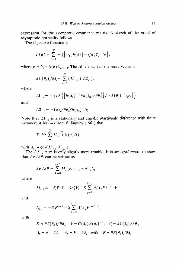
expression for the asymptotic covariance matrix. A sketch of the proof of

asymptotic normality follows.

The objective function is

L(B) = t - :[loglh(O) I- v;h(e)y’l;],

r=1

where v, = Y, - S( 6)X,,,_ i. The i th element of the score vector is

~LUWW = i (LI,,, + L2,,), t=1

where

Ll,,,= -:~~([h(e”)-‘ah(e,)/aei][r-h(e~)-’v,v;])

and

~2,,, = - (av,/aej)~h(eo)~lv,.

Note that Ll,,, is a stationary and ergodic martingale difference with finite variance; it follows from Billingsley (1961) that

Ll, ,” N(0, D), t=l

with d,, = cov( Ll,,,!, Ll,, ,).

The L2,,, term is only slightly more trouble. It is straightforward to show that av,/Jei can be written as

f-2

JvJW= c W,,4v,+Pk+N,,,X,~ k=O

where

k-l

M,,k = -S,FkV- SA,kl/;- S c A;A2Fk-Jp’V J=o

and

r-2

N,_, = -S,Fi-l - S c A,kA2Ft-2pk, k=O

with

s, = as(e,)/ae,, v= G(e,)A(eJ’, r/; = av(e,)/ae,,

A,=F- vs, A,=C- vs, with F;=aF(e,)/ae,,


and the final term in M, k is zero for k = 0. Since both F and A, have eigenvalues which all are less than one in modulus, N, f and M,, k converge to zero at an exponential rate as t and k + cc. This implies that

T-‘12cL2,- T-‘/2xi2,: 0,

where

is a stationary and ergodic martingale difference sequence with finite variance. This implies

T-‘/*xL2, ,” N(0, IV),

with w,, = cov( L2 ;, ,, L2j, ,). If we let ulj denote the covariance between Ll,, t and L2jY,, then T- ‘/‘ilL( 19,)/~30 converges to a normal random vector with mean zero and covariance matrix U, with uiJ = d,j + wiJ + 2v,,.

The usual Taylor series argument expanding T- “*aL( tf~)/t30 about T- ‘I2 8 L (l3,)/80 completes the proof, yielding

T1’2( & - eo) ,” N(0, &),

with Z, = JUJ’, with J-l = plim(T-1a2L(80)/J0&?‘).

References

Akaike, H., 1974, Markovian representation of stochastic processes analysis of autoregressive moving average processes, Annals of Mathematics 20, 363-388.

and its application to the the Institute of Statistical

Anderson, B.D.O. and J.B. Moore, 1979, Optimal filtering (Prentice-Hall, Englewood Cliffs, NJ). Billingsley, P., 1961, The Lindeberg-Levy theorem for martingales, Journal of the American

Mathematical Society 12, 788-792. Blanchard, O.J., 1979, Backward and forward solutions for economies with rational expectations,

American Economic Review 69,114-118. Blanchard, O.J., 1982, Identification in dynamic linear models with rational expectations, HIER

discussion paper no. 888 (Harvard University, Cambridge, MA). Blanchard, O.J.,- 1983, The ‘production and inventory behavior of the American automobile

industrv. Journal of Political Economv 91, 365-400. Blanchard: O.J. and C.M. Kahn, 1980; Solution of linear difference models under rational

expectations, Econometrica 38, 1305-1311. Blanchard, O.J. and M.W. Watson, 1982, Bubbles. rational expectations, and financial markets,

in: Paul Wachtel, ed., Crisis in the economic and financial structure: Bubbles, bursts and shocks (Lexington Books, Lexington, MA).

M. W. W&son, Recursive solufion method 89

Broze, L., C. Gourieroux, and A. Szafan, 1985, Solutions of linear rational expectations models, Econometric Theory 1, 341-368.

Campbell, J. and R.J. Shiller, 1986, Cointegration and tests of present value models, NBER working paper no. 1885.

Chow, G.C., 1983, Econometrics (McGraw-Hill, New York, NY). Diba, B. and H. Grossman, 1983, Rational asset price bubbles, NBER working paper no. 1059. Dunsmuir, W. and E.J. Hannan, 1976, Vector linear time series models, Advances in Applied

Probability 8, 339-364. Engle, R.F. and C.W.J. Granger, 1987, Cointegration and error correction: Representation,

estimation, and testing, Econometrica 55, 251-276. Engle, R.F. and M.W. Watson, 1985, The Kalman filter: Applications to forecasting and rational

expectations models, in: T. Bewley, ed., Advances in econometrics, Fifth world congress (Cambridge University Press, Cambridge).

Flood, R.P. and P.M. Garber, 1980, Market fundamentals versus price-level bubbles: The first tests, Journal of Political Economy 88, 745-780.

Glover, K. and J.C. Willmems, 1974, Paramaterizations of linear dynamical systems: Canonical forms and identifiability, IEEE Transactions on Automatic Control AC-19, 640-645.

Gourieroux, C., J.J. Laffont, and A. Monfort, 1982, Rational expectations in linear models: Analysis of solutions, Econometrica 50, 409-425.

Hansen, L.P. and T.J. Sargent, 1980, Formulating and estimating dynamic linear rational expectations models, Journal of Economic Dynamics and Control 2, 7-46.

Hansen. L.P. and T.J. Sargent, 1982, Instrumental variables procedures for estimating linear rational expectations models, Journal of Monetary Economics 9, 263-296.

Harvey, A.C., 1981, Time series models (Halstead Press, New York, NY). Harvey, A.C. and R.G. Pierse, 1984, Estimating missing observations in economic time series,

Journal of the American Statistical Association 79, 125-131. Harvey, A.C., CR. McKenzie, D.P.C. Blake, and M.J. Desai, 1981, Irregular data revisions, in:

Arnold Zellner, ed., Applied time series analysis of economic data, Economic research report no. ER-5 (U.S. Department of Commerce, Washington, DC).

Hausman, J.A. and M.W. Watson, 1985, Errors-in-variables and seasonal adjustment procedures, Journal of the American Statistical Association 80, 531-540.

McCallum, B.T., 1976, Rational expectations and the natural rate hypothesis: Some consistent estimates, Econometrica 44, 43-52.

Sargent, T.J., 1979, A note on the maximum likelihood estimation of the rational expectations model of the term structure, Journal of Monetary Economics 5, 133-138.

Pesaran, M.H., 1981, Identification of rational expectations models, Journal of Econometrics 16, 375-398.

Schweppe, F., 1965, Evaluation of likelihood functions for Gaussian signals, IEEE Transactions on Information Theory 11, 61-70.

Shiller, R.J., 1981, Do stock prices move too much to be justified by subsequent changes in dividends, American Economic Review 71, 421-436.

Stigum, B.P., 1974, Asymptotic properties of dynamic stochastic parameter estimates III, Journal of Multivariate Analysis 4, 47-88.

Stock, J.H., 1987, Asymptotic properties of least squares estimators of cointegrating vectors, Econometrica 55, 1035-1056.

West, K.D., 1986, Speculative bubbles and stock price volatility, Mimeo. (Princeton University, Princeton, NJ).

Whiteman, C.H., 1983, Linear rational expectations models (University of Minnesota Press, Minneapolis, MN).

Documents

RECURSIVE SOLUTION METHODS FOR DYNAMIC LINEAR RATIONAL