(1.2)(1.2)

(1.1)(1.1)

(1.3)(1.3)

Recursion

Another way to control program flow in Maple is to use recursion. Recursion refers to a function which occurs in its own definition. This concept is well-known to mathematicians who use a lot of recursive definitions. The most famous one is probably the factorial function . Which is defined as

.

We can convert this definition verbatimly into a Maple procedure:

As usual we demonstrate the correctness of the procedure:

Another famous recursive function is the Euclidean algorithm for computing the greatest common divisor of two (positive) integers.

Which computes correctly:

Recursion is usually a divide and conquer approach: In order to solve a problem, first check for simple cases which can be solved immeadiately. If we are not facing a simple case, try to reduce theproblem into smaller problems of a similar shape. In the factorial example, the simple case is ,

(1.4)(1.4)

(2.4)(2.4)

(2.2)(2.2)

(2.1)(2.1)

(2.3)(2.3)

and smaller problem is the computation of instead of the larger problem of computing . The simple cases are usally called base cases. It is important not to forget them. Else the procedure will recurse forever.

Remember our digit sum example. If we want to compute the digit sum of , then this is easy if because then is the only digit. Otherwise, we can reduce the problem to computing the sum

of the last digit and the digit sum of the remaining digits. In code, this looks as follows:

And indeed, this computes the same digit sum as the non-recursive version:

23

We will revisit recursive functions later.

To understand recursion, you must understand recursion or ask somebody who understands recursion.

Exercise: Prove that the Euclidean algorithm really returns a greatest common divisor after finitely many steps.

Exercise: Write a recursive procedure to compute the -th Fibonacci number for .

Data types

Maple distinguishes several types of data. We can for each piece of data inquire its type with the "whattype" function:

fraction

`C `

`*`

string

(2.11)(2.11)

(2.13)(2.13)

(2.5)(2.5)

(2.8)(2.8)

(2.6)(2.6)

(2.10)(2.10)

(2.12)(2.12)

(2.14)(2.14)

(2.9)(2.9)

(2.7)(2.7)

float

integer

Matrix

A full list of types known to Maple can be found in the help system:

We can check whether an expression has a certain type using the "type" function:

true

true

true

false

As we see, a data value can have more than one possible type.

We can be more specific which type we are looking for:

true

false

true

(Note that we have to put "Vector" into single quotes when it is used as a type. Otherwise, Maple willconfuse it with a call to the "Vector" function. The same is true for "Matrix".)

Sequences and Lists

A sequence in Maple is just some expressions separated by commata ",".

(3.4)(3.4)

(3.3)(3.3)

(3.2)(3.2)

(3.1)(3.1)

(3.8)(3.8)

(3.5)(3.5)

(3.9)(3.9)

(3.7)(3.7)

(3.6)(3.6)

(3.10)(3.10)

exprseq

We can assign sequences to a variable:

We can use sequences in procedure calls. Maple will interpret this like the content of the sequence was written in the same place. Thus, if the sequence is the -th argument, then Maple will not assign the complete sequence to the -th formal parameter of the procedure, but instead it will assign the first entry of the sequence to the -th parameter, the second to the -st parameter and so on. For example, since defined above has two entries, the following call corresponds to

where is the first entry of and is the second one.

We can mix sequences and normal parameters.

"a is 1."

We can use sequences in parallel assignments:

In order to access the entries of a sequence, the "[ ]" notation can be used. Note, that counting starts (mathematically) at 1.

(3.14)(3.14)

(3.12)(3.12)

(3.13)(3.13)

(3.16)(3.16)

(3.11)(3.11)

(3.15)(3.15)

Sequences can be generated using the "seq" command. It expects a expression (possibly depending on a parameter) and a range (for that parameter). Optionally a third value can be given which corresponds to the increase of the parameter in each step.

Another form of "seq" allows to access the components of a expression.

Actually, the "in" syntax work also with "add" and "mul" (= multiply):

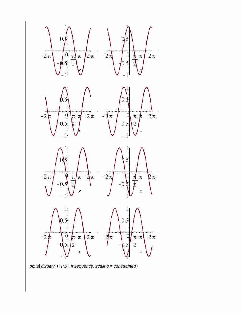
The expression in the first argument of "seq" can be arbitrarily complicated. We have been using this for creating animations. There, the expressions were plots:

(3.23)(3.23)

(3.22)(3.22)

(3.21)(3.21)

(3.19)(3.19)

(3.20)(3.20)

(3.24)(3.24)

(3.17)(3.17)

(3.25)(3.25)

(3.18)(3.18)

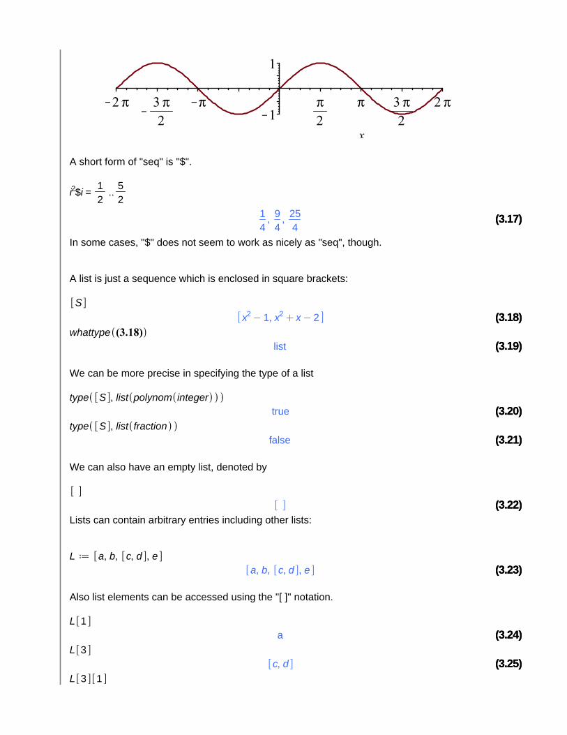
A short form of "seq" is "$".

In some cases, "$" does not seem to work as nicely as "seq", though.

A list is just a sequence which is enclosed in square brackets:

list

We can be more precise in specifying the type of a list

true

false

We can also have an empty list, denoted by

Lists can contain arbitrary entries including other lists:

Also list elements can be accessed using the "[ ]" notation.

a

(3.33)(3.33)

(3.28)(3.28)

(3.32)(3.32)

(3.30)(3.30)

(3.35)(3.35)

(3.37)(3.37)

(3.31)(3.31)

(3.27)(3.27)

(3.34)(3.34)

(3.29)(3.29)

(3.36)(3.36)

(3.26)(3.26)c

The last expression be also be written in the following shorthand form:

c

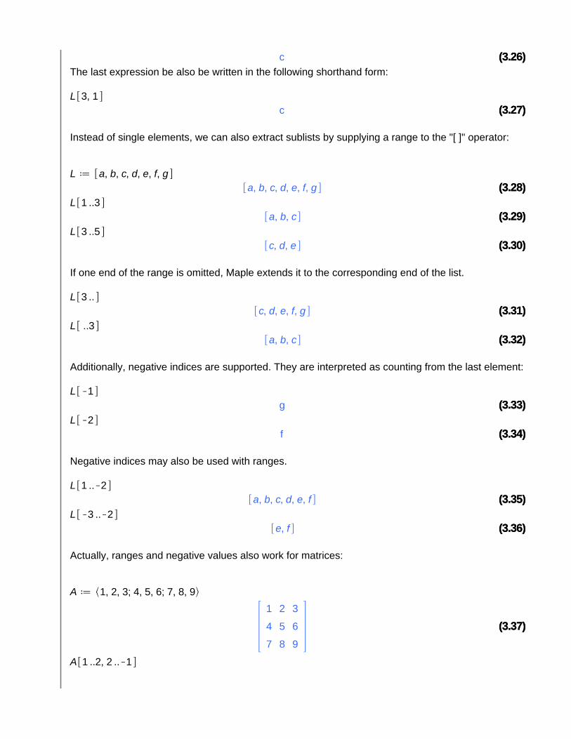
Instead of single elements, we can also extract sublists by supplying a range to the "[ ]" operator:

If one end of the range is omitted, Maple extends it to the corresponding end of the list.

Additionally, negative indices are supported. They are interpreted as counting from the last element:

g

f

Negative indices may also be used with ranges.

Actually, ranges and negative values also work for matrices:

(3.47)(3.47)

(3.39)(3.39)

(3.43)(3.43)

(3.42)(3.42)

(3.41)(3.41)

(3.46)(3.46)

(3.45)(3.45)

(3.44)(3.44)

(3.40)(3.40)

(3.38)(3.38)

(3.48)(3.48)

(3.26)(3.26)

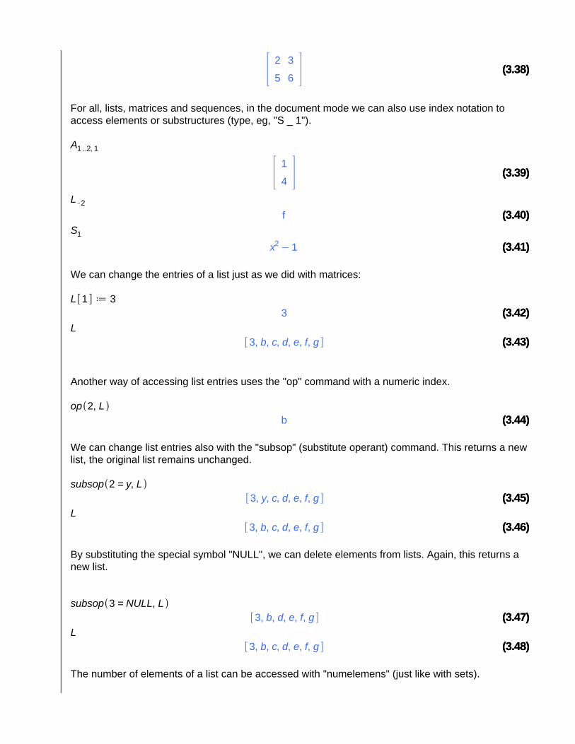
For all, lists, matrices and sequences, in the document mode we can also use index notation to access elements or substructures (type, eg, "S _ 1").

f

We can change the entries of a list just as we did with matrices:

3

Another way of accessing list entries uses the "op" command with a numeric index.

b

We can change list entries also with the "subsop" (substitute operant) command. This returns a new list, the original list remains unchanged.

By substituting the special symbol "NULL", we can delete elements from lists. Again, this returns a new list.

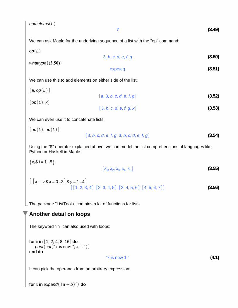
The number of elements of a list can be accessed with "numelemens" (just like with sets).

(3.52)(3.52)

(3.50)(3.50)

(4.1)(4.1)

(3.53)(3.53)

(3.56)(3.56)

(3.54)(3.54)

(3.49)(3.49)

(3.55)(3.55)

(3.51)(3.51)

(3.38)(3.38)

(3.26)(3.26)

7

We can ask Maple for the underlying sequence of a list with the "op" command:

exprseq

We can use this to add elements on either side of the list:

We can even use it to concatenate lists.

Using the "$" operator explained above, we can model the list comprehensions of languages like Python or Haskell in Maple.

The package "ListTools" contains a lot of functions for lists.

Another detail on loops

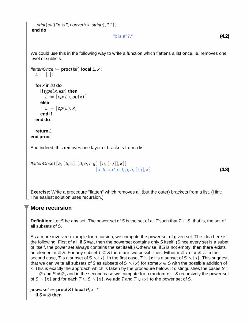
The keyword "in" can also used with loops:

"x is now 1."

It can pick the operands from an arbitrary expression:

(4.3)(4.3)

(4.2)(4.2)

(3.38)(3.38)

(3.26)(3.26)

"x is a^7."

We could use this in the following way to write a function which flattens a list once, ie, removes one level of sublists.

And indeed, this removes one layer of brackets from a list:

Exercise: Write a procedure "flatten" which removes all (but the outer) brackets from a list. (Hint: The easiest solution uses recursion.)

More recursion

Definition: Let be any set. The power set of is the set of all such that , that is, the set of all subsets of .

As a more involved example for recursion, we compute the power set of given set. The idea here is the following: First of all, if , then the powerset contains only itself. (Since every set is a subet of itself, the power set always contains the set itself.) Otherwise, if is not empty, then there exists an element . For any subset there are two possibilities: Either or . In the second case, is a subset of . In the first case, is a subset of . This suggest,that we can write all subsets of as subsets of for some with the possible addition of . This is exactly the approach which is taken by the procedure below. It distinguishes the cases

and , and in the second case we compute for a random recursively the power setof and for each , we add and to the power set of .

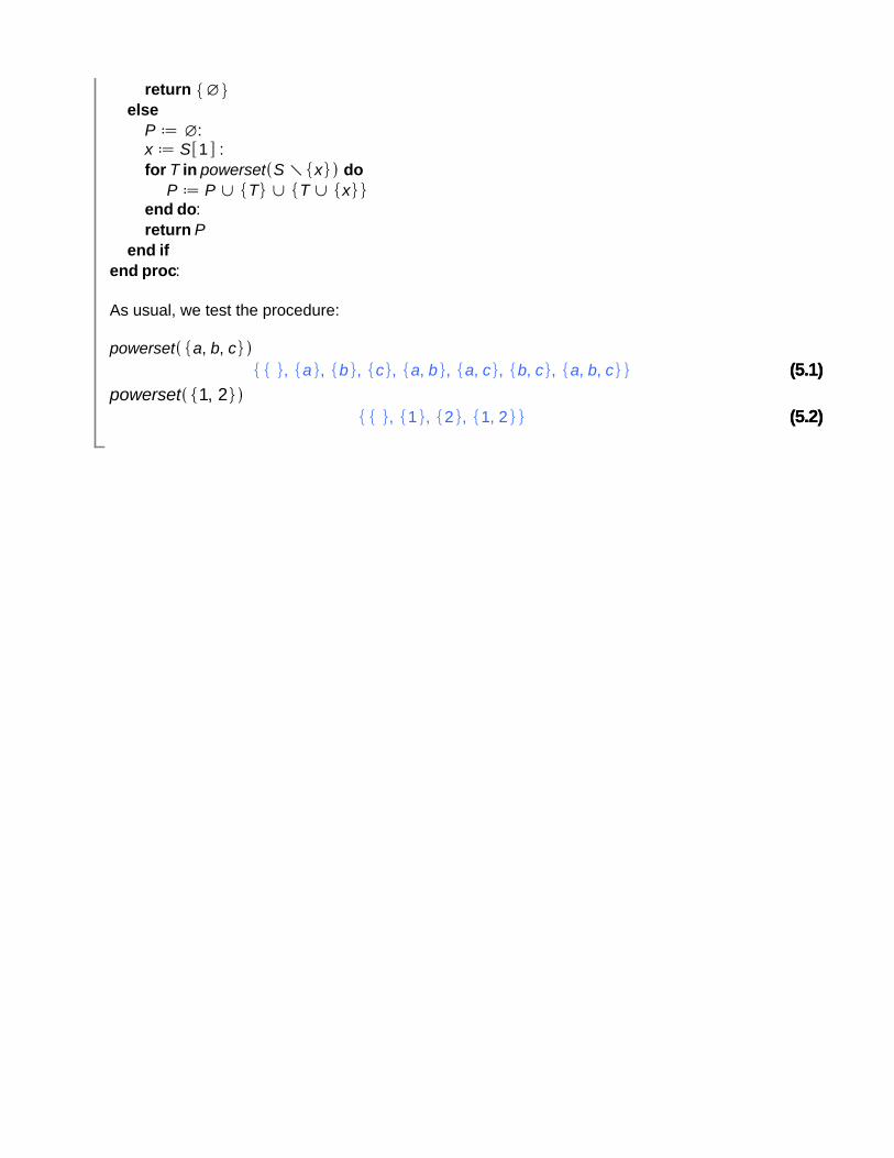
(5.1)(5.1)

(5.2)(5.2)

(3.38)(3.38)

(3.26)(3.26)

As usual, we test the procedure: