Recurrent neural networks and Long-short term memory

(LSTM)

Jeong Min LeeCS3750, University of Pittsburgh

Outline

• RNN• RNN• Unfolding Computational Graph• Backpropagation and weight update• Explode / Vanishing gradient problem

• LSTM• GRU• Tasks with RNN• Software Packages

So far we are

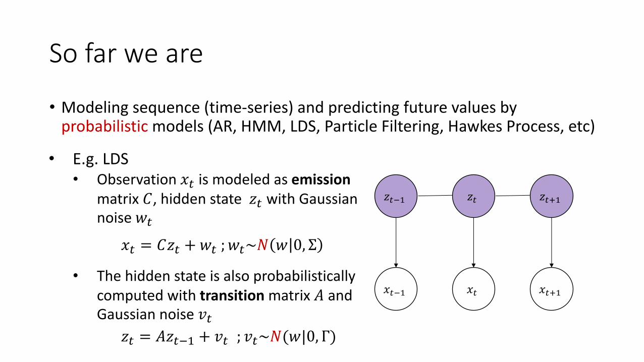
• Modeling sequence (time-series) and predicting future values by probabilistic models (AR, HMM, LDS, Particle Filtering, Hawkes Process, etc)

• E.g. LDS• Observation 𝑥" is modeled as emission

matrix 𝐶, hidden state 𝑧" with Gaussian noise𝑤"

• The hidden state is also probabilistically computed with transition matrix 𝐴 and Gaussian noise 𝑣"

𝑧"()

𝑥"()

𝑧"

𝑥"

𝑧"*)

𝑥"*)

𝑥" = 𝐶𝑧" + 𝑤" ; 𝑤"~𝑁 𝑤 0, Σ

𝑧" = 𝐴𝑧"() + 𝑣" ; 𝑣"~𝑁(𝑤|0, Γ)

Paradigm Shift to RNN

• We are moving into a new world where no probabilistic component exists in a model• That is, we may not need to inference like in LDS and HMM

• In RNN, hidden states bear no probabilistic form or assumption

• Given fixed input and target from data, RNN is to learn intermediate association between them and also the real-valued vector representation

RNN

• RNN’s input, output, and internal representation (hidden states) are all real-valued vectors

ℎ" = tanh 𝑈𝑥𝑡 +𝑊ℎ"()

?𝑦 = λ(𝑉ℎ𝑡)

• ℎ": hidden states; real-valued vector• 𝑥𝑡: input vector (real-valued)• 𝑉ℎ𝑡: real-valued vector• ?𝑦 : output vector (real-valued)

RNN

• RNN consists of three parameter matrices (𝑈, 𝑊,𝑉) with activation functions

ℎ" = tanh 𝑈𝑥𝑡 +𝑊ℎ"()

?𝑦 = λ(𝑉ℎ𝑡)

• 𝑈: input-hidden matrix• 𝑊: hidden-hidden matrix• 𝑉: hidden-output matrix

RNN

• tanh C is a tangent hyperbolic function. It models non-linearity.

ℎ" = tanh 𝑈𝑥𝑡 +𝑊ℎ"()

?𝑦 = λ(𝑉ℎ𝑡)

z

tanh

(z)

RNN

• λ C is output transformation function• It can be any function and selected for a task and type of target in data• It can be even another feed-forward neural network and it makes RNN to

model anything, without any restriction

ℎ" = tanh 𝑈𝑥𝑡 +𝑊ℎ"()

?𝑦 = λ(𝑉ℎ𝑡)

• Sigmoid: binary probability distribution• Softmax: categorical probability distribution• ReLU: positive real-value output• Identity function: real-value output

Make a prediction

• Let’s see how it makes a prediction• In the beginning, initial hidden state ℎD is filled with zero or random value• Also we assume the model is already trained. (we will see how it is trained soon)

𝑥)

ℎD

Make a prediction

• Assume we currently have observation 𝑥1 and want to predict 𝑥2• We compute hidden states ℎ) first

ℎ) = tanh 𝑈𝑥1 +𝑊ℎD

𝑥)

ℎ)ℎD𝑊

𝑈

Make a prediction

• Then we generate prediction:• 𝑉ℎ1 is a real-valued vector or scalar value

(depends on the size of output matrix 𝑉)

ℎ) = tanh 𝑈𝑥1 +𝑊ℎD

?𝑥G = ?𝑦 = λ(𝑉ℎ1)

𝑥) ?𝑥G

ℎ)ℎD𝑊

𝑈

𝑉, λ()

?𝑥G

Make a prediction multiple steps

• In prediction for multiple steps a head, predicted value ?𝑥G from previous step is considered as input 𝑥G at time step 2

ℎG = tanh 𝑈?𝑥G +𝑊ℎ)

?𝑥H = ?𝑦 = λ(𝑉ℎ2)

𝑥) ?𝑥H

ℎ)ℎD𝑊

𝑈

𝑉, λ()

?𝑥G

ℎG𝑊

𝑈

𝑉, λ()

?𝑥H

?𝑥G

Make a prediction multiple steps

• Same mechanism applies forward in time..

ℎH = tanh 𝑈?𝑥H +𝑊ℎG

?𝑥I = ?𝑦 = λ(𝑉ℎ3)

𝑥) ?𝑥H

ℎ)ℎD𝑊

𝑈

𝑉, λ()

?𝑥G

ℎG𝑊

𝑈

𝑉, λ()

?𝑥H

?𝑥G ?𝑥I

ℎH𝑊

𝑈

𝑉, λ()

?𝑥I

RNN Characteristic

• You might observed that…• Parameters 𝑈, 𝑉,𝑊 are shared across all time steps • No probabilistic component (random number generation) is involved• So, everything is deterministic

𝑥) ?𝑥H

ℎ)ℎD𝑊

𝑈

𝑉, λ()

?𝑥G

ℎG𝑊

𝑈

𝑉, λ()

?𝑥H

?𝑥G ?𝑥I

ℎH𝑊

𝑈

𝑉, λ()

?𝑥I

Another way to see RNN

• RNN is a type of neural network

Neural Network

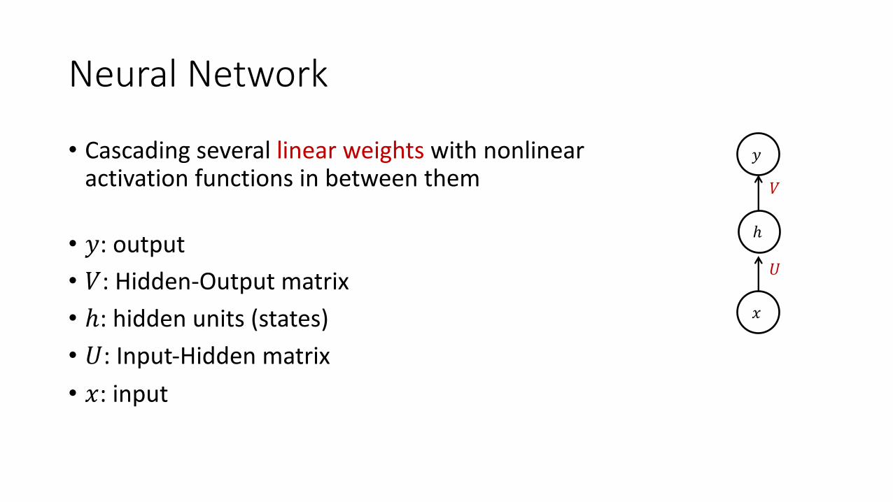
• Cascading several linear weights with nonlinear activation functions in between them

• 𝑦: output• 𝑉: Hidden-Output matrix• ℎ: hidden units (states)• 𝑈: Input-Hidden matrix• 𝑥: input

𝑥

ℎ

𝑦

𝑈

𝑉

Neural Network

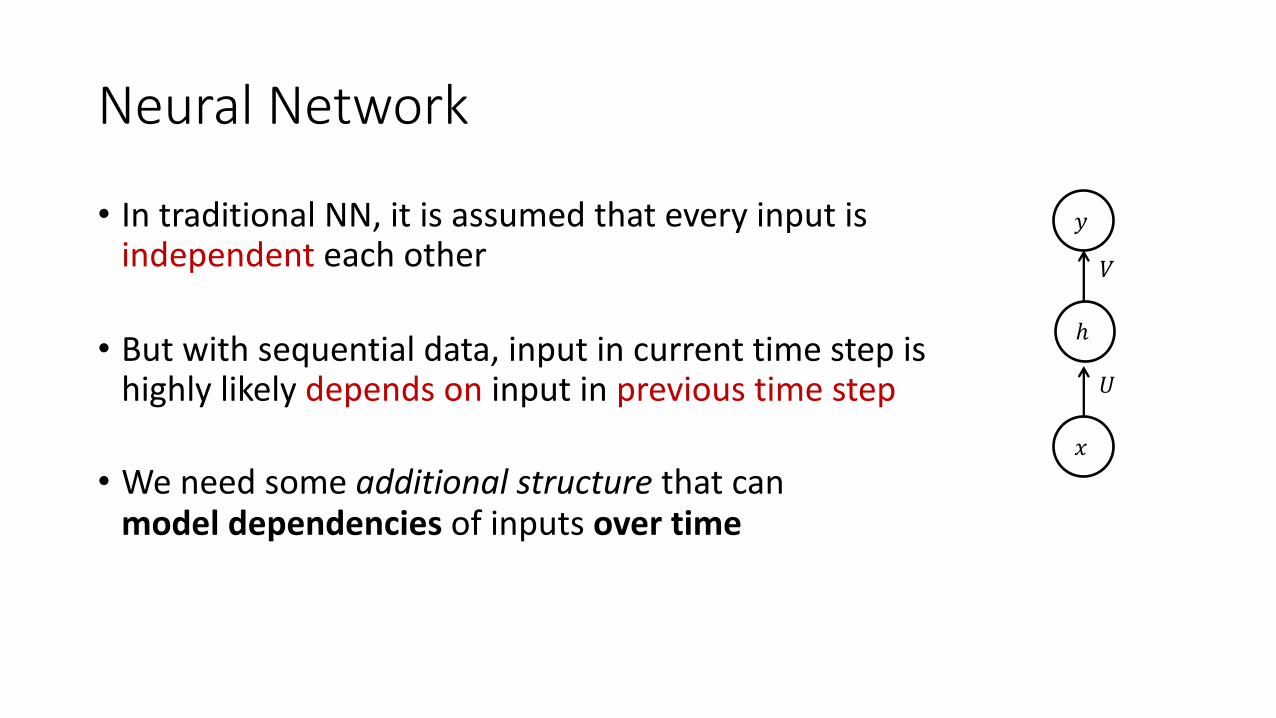
• In traditional NN, it is assumed that every input is independent each other

• But with sequential data, input in current time step is highly likely depends on input in previous time step

• We need some additional structure that can model dependencies of inputs over time

𝑥

ℎ

𝑦

𝑈

𝑉

Recurrent Neural Network

• A type of a neural network that has a recurrence structure• The recurrence structure allows us to operate over a sequence of vectors

𝑥

ℎ

𝑦

𝑈

𝑉 𝑊

RNN as an Unfolding Computational Graph

𝑥

ℎ

𝑦

𝑈

𝑉 𝑊

𝑥"()

ℎ"()

?𝑦"()

𝑈

𝑉

𝑥"

ℎ"

?𝑦"

𝑈

𝑉𝑊

𝑥"*)

ℎ"*)

?𝑦"*)

𝑈

𝑉

ℎ … ℎ …𝑊𝑊 𝑊

Unfold

RNN as an Unfolding Computational Graph

RNN can be converted into a feed-forward neural network by unfolding over time

𝑥

ℎ

𝑦

𝑈

𝑉 𝑊

𝑥"()

ℎ"()

?𝑦"()

𝑈

𝑉

𝑥"

ℎ"

?𝑦"

𝑈

𝑉𝑊

𝑥"*)

ℎ"*)

?𝑦"*)

𝑈

𝑉

ℎ … ℎ …𝑊𝑊 𝑊

Unfold

How to train RNN?

• Before make train happen, we need to define these:• 𝑦𝑡: true target • ?𝑦": output of RNN (=prediction for true target)• 𝐸𝑡: error (loss); difference between the true target and the output

• As the output transformation function 𝜆 is selected by the task and data, so does the loss:

• Binary Classification: Binary Cross Entropy• Categorical Classification: Cross Entropy• Regression: Mean Squared Error

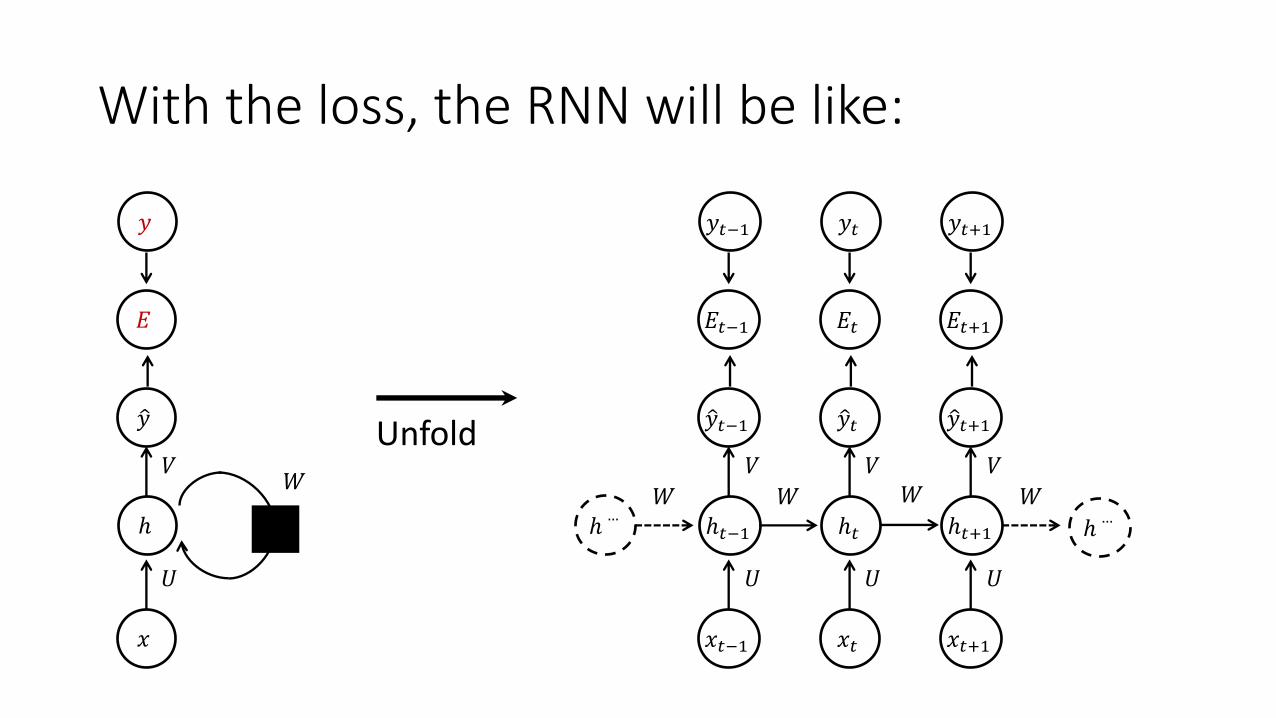
With the loss, the RNN will be like:

Unfold

𝑥"()

ℎ"()

?𝑦"()

𝐸"()

𝑦"()

𝑈

𝑉

𝑥"

ℎ"

?𝑦"

𝐸"

𝑦"

𝑈

𝑉𝑊

𝑥"*)

ℎ"*)

?𝑦"*)

𝐸"*)

𝑦"*)

𝑈

𝑉

ℎ … ℎ …𝑊𝑊 𝑊

𝑥

ℎ

?𝑦

𝐸

𝑦

𝑈

𝑉 𝑊

Back Propagation Through Time (BPTT)

• Extension of standard backpropagation that performs gradient descent on an unfolded network• Goal is to calculate gradients of the error

with respect to parameters U,V,and Wand learn desired parameters using Stochastic Gradient Descent

𝑦G

𝑥1

ℎ1

?𝑦)

𝐸1

𝑈

𝑉𝑊

𝑥2

ℎ2

?𝑦G

𝐸2

𝑈

𝑉𝑊

𝑥3

ℎ3

?𝑦H

𝐸3

𝑈

𝑉

𝑦) 𝑦H

Back Propagation Through Time (BPTT)

• To update in one training example (sequence), we sum up the gradients at each time of the sequence:

𝜕𝐸𝜕𝑊 =T

"

𝜕𝐸𝑡𝜕𝑊

𝑦G

𝑥1

ℎ1

?𝑦)

𝐸1

𝑈

𝑉𝑊

𝑥2

ℎ2

?𝑦G

𝐸2

𝑈

𝑉𝑊

𝑥3

ℎ3

?𝑦H

𝐸3

𝑈

𝑉

𝑦) 𝑦H

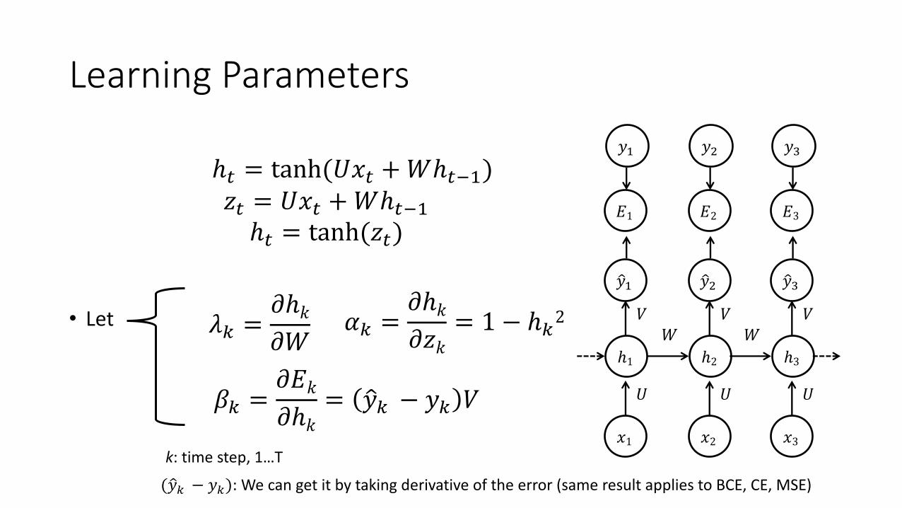
Learning Parameters

• Let

ℎ" = tanh(𝑈𝑥" +𝑊ℎ"())𝑧" = 𝑈𝑥" +𝑊ℎ"()ℎ" = tanh(𝑧")

𝜆U =𝜕ℎ𝑘𝜕𝑊

𝛼U =𝜕ℎ𝑘𝜕𝑧𝑘

= 1 − ℎU2

𝛽U =𝜕𝐸𝑘𝜕ℎ𝑘

= ?𝑦U − 𝑦U 𝑉

𝑦G

𝑥1

ℎ1

?𝑦)

𝐸1

𝑈

𝑉𝑊

𝑥2

ℎ2

?𝑦G

𝐸2

𝑈

𝑉𝑊

𝑥3

ℎ3

?𝑦H

𝐸3

𝑈

𝑉

𝑦) 𝑦H

k: time step, 1…T

( ?𝑦U − 𝑦U): We can get it by taking derivative of the error (same result applies to BCE, CE, MSE)

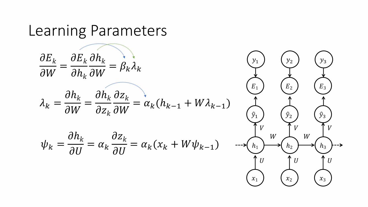
Learning Parameters𝜕𝐸𝑘𝜕𝑊 =

𝜕𝐸𝑘𝜕ℎ𝑘

𝜕ℎ𝑘𝜕𝑊 = 𝛽U𝜆U

𝜓U =𝜕ℎ𝑘𝜕𝑈 = 𝛼U

𝜕𝑧𝑘𝜕𝑈 = 𝛼U(𝑥U +𝑊𝜓U())

𝜆U =𝜕ℎ𝑘𝜕𝑊 =

𝜕ℎ𝑘𝜕𝑧𝑘

𝜕𝑧𝑘𝜕𝑊 = 𝛼U(ℎU() +𝑊𝜆U())

𝑦G

𝑥1

ℎ1

?𝑦)

𝐸1

𝑈

𝑉𝑊

𝑥2

ℎ2

?𝑦G

𝐸2

𝑈

𝑉𝑊

𝑥3

ℎ3

?𝑦H

𝐸3

𝑈

𝑉

𝑦) 𝑦H

𝜓U = 𝛼U(𝑥U +𝑊𝜓U())

𝛼D = 1 − ℎD2; 𝜆D = 0; 𝜓D = 𝛼D C 𝑥DΔ𝑤 = 0 ; Δ𝑢 = 0 ; Δ𝑣 = 0For k= 1...T (T; length of a sequence):

𝛼U = 1 − ℎU2

𝜆U = 𝛼U(ℎU() +𝑊𝜆U())𝛽U = ?𝑦" − 𝑦U 𝑉Δ𝑤 = Δ𝑤 + 𝛽U𝜆U

Δ𝑢 = Δ𝑢 + 𝛽U𝜓UΔ𝑣 = Δ𝑣 + ?𝑦" − 𝑦U ⊗ ℎU

Initialization:

𝑉𝑛𝑒𝑤 = 𝑉𝑜𝑙𝑑 − 𝛼Δ𝑣𝑊𝑛𝑒𝑤 = 𝑊𝑜𝑙𝑑 − 𝛼Δ𝑤𝑈𝑛𝑒𝑤 = 𝑈𝑜𝑙𝑑 − 𝛼Δ𝑢

𝛼: learning rate⊗: element-wise multiplication

Then,

Exploding and Vanishing Gradient Problem

• In RNN, we repeatedly multiply W along with a input sequence

• The recurrence multiplication can result in difficulties called exploding and vanishing gradient problem

ℎ" = tanh(𝑈𝑥𝑡 +𝑊ℎ"())

𝑦G

𝑥1

ℎ1

?𝑦)

𝐸1

𝑈

𝑉𝑊

𝑥2

ℎ2

?𝑦G

𝐸2

𝑈

𝑉𝑊

𝑥3

ℎ3

?𝑦H

𝐸3

𝑈

𝑉

𝑦) 𝑦H

Exploding and Vanishing Gradient Problem

• For example, we can think of simple RNN with lacking inputs 𝒙

• It can be simplified to

• If 𝑊 has an Eigen decomposition, we can decompose 𝑊 into 𝑉 (consists of eigen vectors) and a diagonal matrix of eigen values: diag 𝜆

ℎ𝑡 = (𝑊𝑡)ℎ0

ℎ𝑡 = 𝑊ℎ"()

𝑊 = 𝐴 diag 𝜆 𝐴()

𝑊" = (𝐴 diag 𝜆 𝐴())"= 𝐴 diag 𝜆" 𝐴()

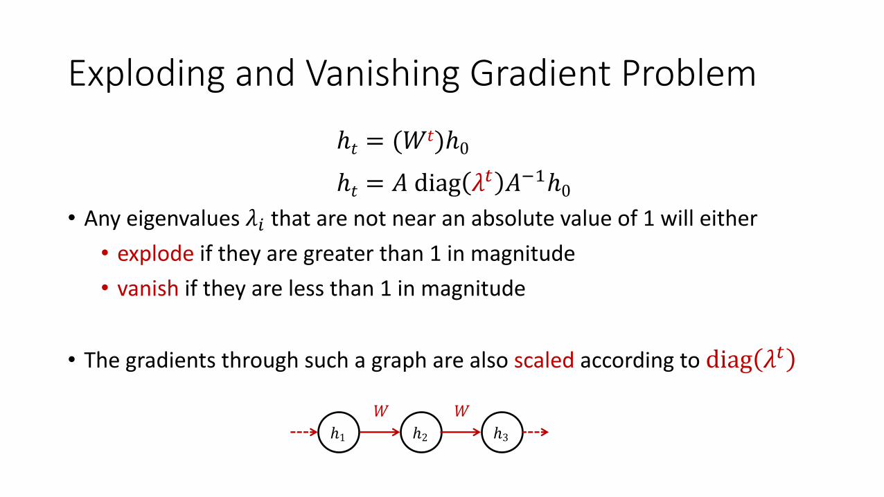
Exploding and Vanishing Gradient Problem

• Any eigenvalues 𝜆f that are not near an absolute value of 1 will either • explode if they are greater than 1 in magnitude • vanish if they are less than 1 in magnitude

• The gradients through such a graph are also scaled according to diag 𝜆"

ℎ1𝑊

ℎ2𝑊

ℎ3

ℎ𝑡 = 𝐴 diag 𝜆" 𝐴()ℎ0

ℎ𝑡 = (𝑊𝑡)ℎ0

Exploding and Vanishing Gradient Problem

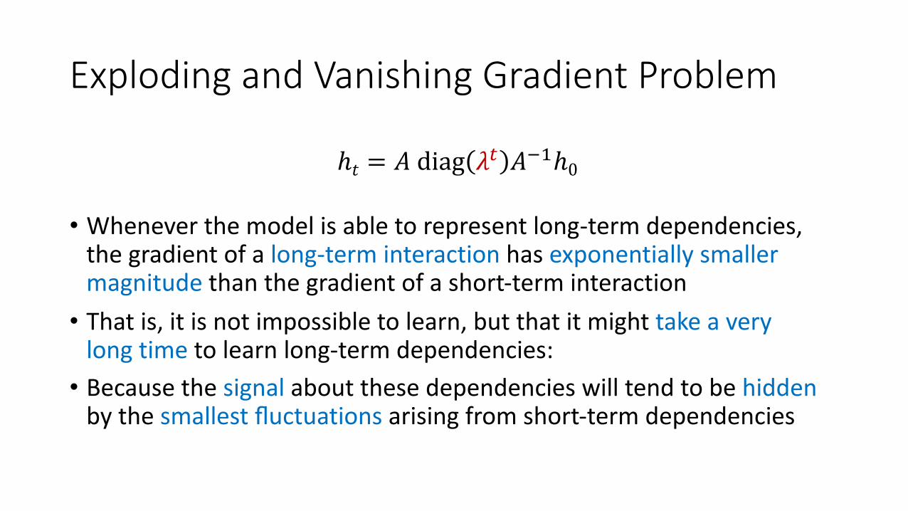
• Whenever the model is able to represent long-term dependencies, the gradient of a long-term interaction has exponentially smaller magnitude than the gradient of a short-term interaction• That is, it is not impossible to learn, but that it might take a very

long time to learn long-term dependencies:• Because the signal about these dependencies will tend to be hidden

by the smallest fluctuations arising from short-term dependencies

ℎ𝑡 = 𝐴 diag 𝜆" 𝐴()ℎ0

Vanishing Gradient • Tanh function has derivatives of 0 at both

ends. (They approach a flat line)• When this happens we say the

corresponding neurons are saturated. • They have a zero gradient and drive other

gradients in previous layers towards 0. • Thus, with small values in the matrix and

multiple matrix multiplications the gradient values are shrinking exponentially fast, eventually vanishing completely after a few time steps. [WildML 2015]

Tanh f(x) and its derivative

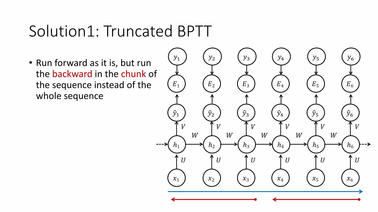
Solution1: Truncated BPTT

• Run forward as it is, but run the backward in the chunk of the sequence instead of the whole sequence

𝑦G

𝑥1

ℎ1

?𝑦)

𝐸1

𝑈

𝑉𝑊

𝑥2

ℎ2

?𝑦G

𝐸2

𝑈

𝑉𝑊

𝑥3

ℎ3

?𝑦H

𝐸3

𝑈

𝑉𝑊

𝑦) 𝑦H 𝑦g

𝑥4

ℎ4

?𝑦I

𝐸4

𝑈

𝑉𝑊

𝑥5

ℎ5

?𝑦g

𝐸5

𝑈

𝑉𝑊

𝑥6

ℎ6

?𝑦k

𝐸6

𝑈

𝑉

𝑦I 𝑦k

Solution2: Gating mechanism (LSTM;GRU)

• Add gates to produce paths where gradients can flow more constantly in longer-term without vanishing nor exploding• We’ll see in next chapter

Outline

• RNN• LSTM• GRU• Tasks with RNN• Software Packages

Long Short-term Memory (LSTM)

• Capable of modeling longer term dependencies by having memory cells and gates that controls the information flow along with the memory cells

Long Short-term Memory (LSTM)

• Capable of modeling longer term dependencies by having memory cells and gates that controls the information flow along with the memory cells

Images: http://colah.github.io/posts/2015-08-Understanding-LSTMs/

Long Short-term Memory (LSTM)

• The contents of the memory cells 𝐶" are regulated by various gates:• Forget gate 𝑓"• Input gate 𝑖"• Reset gate 𝑟"• Output gate 𝑜"

• Each gates are composed of affine transformation with Sigmoid activation function

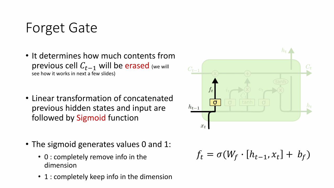
Forget Gate

• It determines how much contents from previous cell 𝐶"() will be erased (we will see how it works in next a few slides)

• Linear transformation of concatenated previous hidden states and input are followed by Sigmoid function

• The sigmoid generates values 0 and 1:• 0 : completely remove info in the

dimension• 1 : completely keep info in the dimension

𝑓" = 𝜎(𝑊p C ℎ"(), 𝑥" + 𝑏p)

New Candidate Cell and Input Gate

• New candidate cell states r𝐶" are created as a function of ℎ"() and 𝑥"

• Input gates 𝑖" decides how much of values of the new candidate cell states r𝐶" are combined into the cell states

r𝐶" = tanh(𝑊s C ℎ"(), 𝑥" + 𝑏s)𝑖" = 𝜎(𝑊f C ℎ"(), 𝑥" + 𝑏f)

Update Cell States

• The previous cell states 𝐶"() are updated to the new cell states 𝐶" by using the input and forget gates with new candidate cell states

𝐶" = 𝑓" ⊗ 𝐶"() + 𝑖" ⊗ r𝐶"

forget gate input gate

previous cell states new cell candidate

⊗: element-wise multiplication

Generate Output

• Output will be based on cell state 𝐶"with filter from output gate 𝑜"• The output gate 𝑜" decides which part

of cell state 𝐶" will be in the output

• Then the final output is generated from tanh-ed cell states filtered by 𝑜"

ℎ" = 𝑜" ⊗ tanh 𝐶"

𝑜" = 𝜎(𝑊t C ℎ"(), 𝑥" + 𝑏t)

Outline

• RNN• LSTM• GRU• Tasks with RNN• Software Packages

Gated Recurrent Unit (GRU)

• Simplify LSTM by merging forget and input gate into update gate 𝑧"• 𝑧" controls the forgetting factor and the decision to update the state unit

ℎ" = 1 − 𝑧" ⊗ ℎ"() + 𝑧" ⊗ uℎ"

𝑧" = 𝜎(𝑊v C ℎ"(), 𝑥" + 𝑏v)

𝑟" = 𝜎(𝑊w C ℎ"(), 𝑥" + 𝑏w)

uℎ" = tanh 𝑊 C 𝑟" ⊗ ℎ"(), 𝑥" + 𝑏

• Reset gates 𝑟" control which parts of the state get used to compute the next target state• It introduces additional nonlinear effect in the relationship between

past state and future state

Gated Recurrent Unit (GRU)

ℎ" = 1 − 𝑧" ⊗ ℎ"() + 𝑧" ⊗ uℎ"

𝑧" = 𝜎(𝑊v C ℎ"(), 𝑥" + 𝑏v)

𝑟" = 𝜎(𝑊w C ℎ"(), 𝑥" + 𝑏w)

uℎ" = tanh 𝑊 C 𝑟" ⊗ ℎ"(), 𝑥" + 𝑏

Comparison LSTM and GRU

ℎ" = 1 − 𝑧" ⊗ ℎ"() + 𝑧" ⊗ uℎ"

𝑧" = 𝜎(𝑊v C ℎ"(), 𝑥" + 𝑏v)

𝑟" = 𝜎(𝑊w C ℎ"(), 𝑥" + 𝑏w)

uℎ" = tanh 𝑊 C 𝑟" ⊗ ℎ"(), 𝑥" + 𝑏

𝑓" = 𝜎(𝑊p C ℎ"(), 𝑥" + 𝑏p)r𝐶" = tanh(𝑊s C ℎ"(), 𝑥" + 𝑏s)𝑖" = 𝜎(𝑊f C ℎ"(), 𝑥" + 𝑏f)

𝐶" = 𝑓" ∗ 𝐶"() + 𝑖"𝑣 r𝐶"

ℎ" = 𝑜" ⊗ tanh 𝐶"

𝑜" = 𝜎(𝑊t C ℎ"(), 𝑥" + 𝑏t)

LSTM GRU

ℎ"()

𝐶"() 𝐶"

ℎ"

ℎ"

𝑥"

Comparison LSTM and GRU

• Greff, et al. (2015) compared LSTM, GRU and several variants on thousands of experiments and found that none of the variants can improve upon the standard LSTM architecture significantly, but also the variants do not decrease performance significantly.

• Greff, et al. (2015): LSTM: A Search Space Odyssey

Outline

• RNN• LSTM• GRU• Tasks with RNN

• One-to-Many• Many-to-One• Many-to-Many• Encoder-Decoder Seq2Seq Model• Attention Mechanism• Bidirectional RNN

• Software Packages

Tasks with RNN

• One of strengths of RNN is flexibility in modeling any task with any data type

• By composing the input and output as either sequential or non-sequential data, you can model many different tasks

• Here are some of the examples:

One-to-Many

• Input: non-sequence vector / Output: sequence of vectors• After the first time step, hidden states are updated with

only previous step’s hidden states• Example: Sentence generation given image• Typically the input image is processed with CNN to generate

a real-valued vector representation• During training, true target is a sentence (sequence of

words) about the training imageInput

Output

Many-to-One

• Input: sequence of vectors / Output: non-sequence vector• Only the last time step’s hidden states is used as the

output• Example: Sequence classification, sentiment classification

Many-to-Many

• Input: sequence of vectors / Output: sequence of vectors• Generate a sequence given another sequence• Example: Machine translation

• Especially parameterized by what is called “Encoder-Decoder” model

• Key idea:• Encoder RNN generates a fixed-length context vector 𝐶

from input sequence 𝑿 = (𝑥 ) , … , 𝑥 z{ )• Decoder RNN generates an output sequence 𝒀 = (𝑦 ) , … , 𝑦 z} ) conditioned on the context 𝐶

• The two RNNs are trained jointly to maximize the average of log𝑃(𝑦 ) , … , 𝑦 z} |𝑥 ) , … , 𝑥 z{ ) over all sequence in training set

Encoder-Decoder (Seq2Seq) Model

• Typically, the last hidden states of encoder RNN ℎ z{ is used as context 𝐶• But when the context 𝐶 has smaller dimension or lengths of

sequences are longer, 𝐶 can be a bottleneck; it cannot properly summarize the input sequence

Encoder-Decoder (Seq2Seq) Model

𝑥 ) 𝑥 G 𝑥 H … 𝑥 z{

ℎ ) ℎ G ℎ H … ℎ z{ 𝑔 ) 𝑔 G 𝑔 H … 𝑔 z}

?𝑦 ) ?𝑦 G ?𝑦 H … ?𝑦 z}

𝐶

Decoder RNN

Encoder RNN

Input sequence

Target sequence

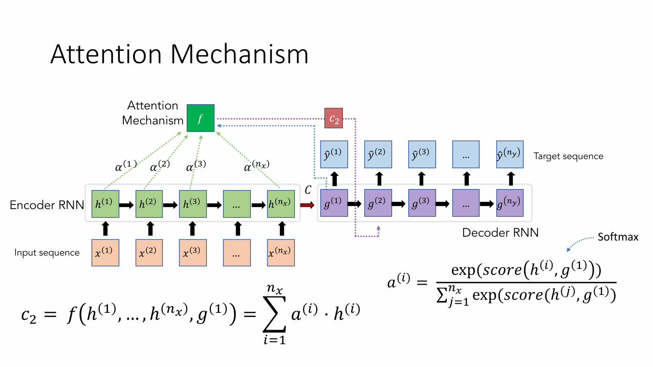
• Attention mechanism learns to associate hidden states of input sequence to generation of each step of the target sequence

Attention Mechanism

𝑥 ) 𝑥 G 𝑥 H … 𝑥 z{

ℎ ) ℎ G ℎ H … ℎ z{ 𝑔 ) 𝑔 G 𝑔 H … 𝑔 z}

?𝑦 ) ?𝑦 G ?𝑦 H … ?𝑦 z}

𝐶

Decoder RNN

Encoder RNN

Input sequence

Target sequence

𝑓Attention

Mechanism 𝑐G

𝛼 ) 𝛼 G 𝛼 H 𝛼 z{

(Input to RNN)

• The association is modeled as additional feed-forward network 𝑓 gets input sequence’s hidden states and predicted target on previous time step

Attention Mechanism

𝑥 ) 𝑥 G 𝑥 H … 𝑥 z{

ℎ ) ℎ G ℎ H … ℎ z{ 𝑔 ) 𝑔 G 𝑔 H … 𝑔 z}

?𝑦 ) ?𝑦 G ?𝑦 H … ?𝑦 z}

𝐶

Decoder RNN

Encoder RNN

Input sequence

Target sequence

𝑓Attention

Mechanism 𝑐G

𝛼 ) 𝛼 G 𝛼 H 𝛼 z{

𝑐G = 𝑓(ℎ ) , … , ℎ z{ , 𝑔()))(Input to RNN)

Attention Mechanism

𝑥 ) 𝑥 G 𝑥 H … 𝑥 z{

ℎ ) ℎ G ℎ H … ℎ z{ 𝑔 ) 𝑔 G 𝑔 H … 𝑔 z}

?𝑦 ) ?𝑦 G ?𝑦 H … ?𝑦 z}

𝐶

Decoder RNN

Encoder RNN

Input sequence

Target sequence

𝑓Attention

Mechanism 𝑐G

𝛼 ) 𝛼 G 𝛼 H 𝛼 z{

𝑐G = 𝑓 ℎ ) , … , ℎ z{ , 𝑔 ) =Tf�)

z{

𝑎(f) ⋅ ℎ(f)

(Input to RNN)

Attention Mechanism

𝑥 ) 𝑥 G 𝑥 H … 𝑥 z{

ℎ ) ℎ G ℎ H … ℎ z{ 𝑔 ) 𝑔 G 𝑔 H … 𝑔 z}

?𝑦 ) ?𝑦 G ?𝑦 H … ?𝑦 z}

𝐶

Decoder RNN

Encoder RNN

Input sequence

Target sequence

𝑓Attention

Mechanism 𝑐G

𝛼 ) 𝛼 G 𝛼 H 𝛼 z{

𝑐G = 𝑓 ℎ ) , … , ℎ z{ , 𝑔 ) =Tf�)

z{

𝑎(f) ⋅ ℎ(f)𝑎(f) =

exp(𝑠𝑐𝑜𝑟𝑒 ℎ f , 𝑔 ) )∑��)z{ exp(𝑠𝑐𝑜𝑟𝑒(ℎ � , 𝑔 ) )

Softmax

Attention Mechanism

𝑥 ) 𝑥 G 𝑥 H … 𝑥 z{

ℎ ) ℎ G ℎ H … ℎ z{ 𝑔 ) 𝑔 G 𝑔 H … 𝑔 z}

?𝑦 ) ?𝑦 G ?𝑦 H … ?𝑦 z}

𝐶

Decoder RNN

Encoder RNN

Input sequence

Target sequence

𝑓Attention

Mechanism 𝑐G

𝛼 ) 𝛼 G 𝛼 H 𝛼 z{

𝑐G = 𝑓 ℎ ) , … , ℎ z{ , 𝑔 ) =Tf�)

z{

𝑎(f) ⋅ ℎ(f)

𝑠𝑐𝑜𝑟𝑒 ℎ f , 𝑔 ) = 𝑣� ⋅ tanh(𝑊� ⋅ [ℎ f , 𝑔 ) ])

𝑎(f) =exp(𝑠𝑐𝑜𝑟𝑒 ℎ f , 𝑔 ) )

∑��)z{ exp(𝑠𝑐𝑜𝑟𝑒(ℎ � , 𝑔 ) )

Softmax

*Same computation procedure is applied to each time step of target

Outline

• RNN• LSTM• GRU• Encoder-Decoder Seq2Seq Model• Bidirectional RNN• Software Packages

• In some applications, such as speech recognition or machine translation, dependencies over time not only lie in forward in time but also lie in backward in time • It assumes all-time step of a sequence is available

Bidirectional RNN

Image: https://distill.pub/2017/ctc/

• To model these, two RNNs are trained together forward RNN and backward RNN• Each time step’s hidden states from both RNNs are concatenated to form

a final output

Bidirectional RNN

ℎ# ℎ$ ℎ%

&# &$ &%

ℎ'

&($ &() &(%*#

ℎ# ℎ$ ℎ% ℎ'…

…

forward RNN

backward RNN

• In many cases, a sequence could have (latent) hierarchical structures. • Example:• Document ➝ Paragraphs ➝ Sentences ➝ Words ➝ Characters• Video ➝ Shots ➝ Still frames

Hierarchical RNNVideo as multiple shots

Shot #1

Shot #2

Shot #k

Shot #k+1

A video

• The straightforward approach is to stack hidden states in several layers.

Hierarchical RNN

ℎ"# ℎ$# ℎ%#ℎ&#

()$ ()* ()%+"

ℎ"" ℎ$" ℎ%"

(" ($ (%

ℎ&"

… … …

…

…

ℎ"# ℎ$# ℎ%#ℎ&#

()$ ()* ()%+"

ℎ"" ℎ$" ℎ%"

(" ($ (%

ℎ&"

… … …

…

…

• One of key research question is to detect where a segment finishes and starts• E.g.,

• Boundaries of words (in a sequence of character)

• Boundaries of scenes (in a sequence of image frames)

• Many works attempted to train models that detect these boundaries

Hierarchical RNN

?

• Video[HSA-RNN: Hierarchical Structure-Adaptive RNN for Video Summarization, Zhao 2018]• Two Layer-Approach

• First layer learns to segment a video into several shots

• Second layer captures forward & backward dependencies among the boundary frames

Hierarchical RNN

• Text [Hierarchical Multiscale Recurrent Neural Networks, Chung 2016]• Hidden states at each level are updated based

on (learned) structure of a sequence• Higher-level hidden states are only update when a

segment finishes• Lower-level hidden states uses higher-level hidden

states info when a new segment is started

Hierarchical RNN

Outline

• RNN• LSTM• GRU• Tasks with RNN• Software Packages

• Many recent Deep Learning packages are supporting RNN/LSTM/GRU:

• PyTorch: https://pytorch.org/docs/stable/nn.html#recurrent-layers• TensorFlow: https://www.tensorflow.org/tutorials/sequences/recurrent• Caffe2: https://caffe2.ai/docs/RNNs-and-LSTM-networks.html• Keras: https://keras.io/layers/recurrent/

• Especially I recommend this for beginner: “Sequence classification on PyTorch (character-level name -> Language)”https://pytorch.org/tutorials/intermediate/char_rnn_classification_tutorial.html

Software Packages for RNN

• A Critical Review of Recurrent Neural Networks for Sequence Learning https://arxiv.org/pdf/1506.00019.pdf• The Unreasonable Effectiveness of Recurrent Neural Networks

http://karpathy.github.io/2015/05/21/rnn-effectiveness/• Understanding LSTM Networks

http://colah.github.io/posts/2015-08-Understanding-LSTMs/• LSTM: A Search Space Odyssey

https://arxiv.org/pdf/1503.04069.pdf• [WildML 2015] Recurrent Neural Networks Tutorial, Part 3 –

Backpropagation Through Time and Vanishing Gradients http://www.wildml.com/2015/10/recurrent-neural-networks-tutorial-part-3-backpropagation-through-time-and-vanishing-gradients/• [Green and Perek 2018] : http://www.master-

taid.ro/Cursuri/MLAV_files/10_MLAV_En_Recurrent_2018.pdf

References

Thank you!

Any questions?