Embed Size (px)
Citation preview


1
0
-1
Z
-3
-0
3
Y
3
-0
-3
X
plot3d1 : z=sin(x)*cos(y)
1.0 1.4 1.8 2.2 2.6 3.0 3.4 3.8 4.2 4.6 5.0
1.0
1.9
2.8
3.7
4.6
5.5
6.4
7.3
8.2
9.1
10.0
0.19
0.19
0.19
0.190.37
0.37
0.37
0.37
0.37
0.37
0.37
0.37
0.37
0.56
0.56
0.56
0.56
0.56
0.56
0.56
0.56
0.56
0.56
0.75
0.75
0.75
0.75
0.75
0.75
0.75
contour
champ
-0.8
-0.8-0.8
-0.6
-0.6-0.6
-0.4
-0.4 -0.4
-0.2
-0.2 -0.20.0
0.0
0.0 0.2
0.2
0.2
0.4
0.4
0.4
0.6
0.6
0.6
0.8
0.8
0.8
Z
YX
plot3d and contour
Introduction
To
Scilab
User's Guide
Scilab Group
-->plot(1:10)
-->xbasc()
-->// simple rectangle
-->xrect(0,1,3,1)
-->// filling a rectangle
-->xfrect(3.1,1,3,1)
-->// writing in the rectangle
-->xstring(0.5,0.5,"xrect(0,1,3,1)")
-->// writing black on black !
-->xstring(4.,0.5,"xfrect(3.1,1,3,1)")
-->// reversing the video
-->xset("alufunction",6)
-->xstring(4.,0.5,"xfrect(3.1,1,3,1)")
-->xset("alufunction",3)
-->// drawing a polyline
-->X=[0 1 2 3 4];
-->Y=[2.5 1.5 1.8 1.3 2.5];
-->xpoly(X,Y,"lines",1)
-->xstring(0.5,2.,"xpoly(X,Y,""lines""
-->// drawing arrows

INTRODUCTION
TO
Lab
Scilab GroupINRIA Meta2 Project/ENPC Cergrene
INRIA - Unit�e de recherche de Rocquencourt - Projet Meta2Domaine de Voluceau - Rocquencourt - B.P. 105 - 78153 Le Chesnay Cedex (France)E-mail : [email protected]


Contents
1 Introduction 1
1.1 What is Scilab : : : : : : : : : : : : : : : : : : : : : : : : : : : : : : : : : : 11.2 Software Organization : : : : : : : : : : : : : : : : : : : : : : : : : : : : : : 21.3 Installing Scilab. System Requirements : : : : : : : : : : : : : : : : : : : : 41.4 Scilab at a Glance. A Tutorial : : : : : : : : : : : : : : : : : : : : : : : : : 4
1.4.1 Getting Started : : : : : : : : : : : : : : : : : : : : : : : : : : : : : : 41.4.2 Editing a command line : : : : : : : : : : : : : : : : : : : : : : : : : 51.4.3 Buttons : : : : : : : : : : : : : : : : : : : : : : : : : : : : : : : : : : 61.4.4 Customizing your Scilab : : : : : : : : : : : : : : : : : : : : : : : : : 61.4.5 Sample Session for Beginners : : : : : : : : : : : : : : : : : : : : : : 7
2 Data Types 19
2.1 Special Constants : : : : : : : : : : : : : : : : : : : : : : : : : : : : : : : : : 192.2 Constant Matrices : : : : : : : : : : : : : : : : : : : : : : : : : : : : : : : : 192.3 Matrices of Character Strings : : : : : : : : : : : : : : : : : : : : : : : : : : 242.4 Polynomials and Polynomial Matrices : : : : : : : : : : : : : : : : : : : : : 272.5 Boolean Matrices : : : : : : : : : : : : : : : : : : : : : : : : : : : : : : : : : 282.6 Lists, Linear Systems : : : : : : : : : : : : : : : : : : : : : : : : : : : : : : : 292.7 Functions (Macros) : : : : : : : : : : : : : : : : : : : : : : : : : : : : : : : : 352.8 Libraries : : : : : : : : : : : : : : : : : : : : : : : : : : : : : : : : : : : : : : 362.9 Objects : : : : : : : : : : : : : : : : : : : : : : : : : : : : : : : : : : : : : : 36
3 Programming 37
3.1 Programming Tools : : : : : : : : : : : : : : : : : : : : : : : : : : : : : : : : 373.1.1 Comparison Operators : : : : : : : : : : : : : : : : : : : : : : : : : : 373.1.2 Loops : : : : : : : : : : : : : : : : : : : : : : : : : : : : : : : : : : : 383.1.3 Conditionals : : : : : : : : : : : : : : : : : : : : : : : : : : : : : : : 39
3.2 De�ning and Using Functions : : : : : : : : : : : : : : : : : : : : : : : : : : 403.2.1 Function Structure : : : : : : : : : : : : : : : : : : : : : : : : : : : : 403.2.2 Loading Functions : : : : : : : : : : : : : : : : : : : : : : : : : : : : 413.2.3 Global and Local Variables : : : : : : : : : : : : : : : : : : : : : : : 413.2.4 Special Function Commands : : : : : : : : : : : : : : : : : : : : : : 43
3.3 De�nition of Operations on New Data Types : : : : : : : : : : : : : : : : : 443.4 Debbuging : : : : : : : : : : : : : : : : : : : : : : : : : : : : : : : : : : : : : 47
4 Basic Primitives 48
4.1 The Environment and Input/Output : : : : : : : : : : : : : : : : : : : : : : 484.1.1 The Environment : : : : : : : : : : : : : : : : : : : : : : : : : : : : : 48
i

ii
4.1.2 Startup Commands by the User : : : : : : : : : : : : : : : : : : : : : 484.1.3 Input and Output : : : : : : : : : : : : : : : : : : : : : : : : : : : : 49
4.2 Help : : : : : : : : : : : : : : : : : : : : : : : : : : : : : : : : : : : : : : : : 494.3 Nonlinear Calculation : : : : : : : : : : : : : : : : : : : : : : : : : : : : : : 49
4.3.1 Externals : : : : : : : : : : : : : : : : : : : : : : : : : : : : : : : : : 494.3.2 Nonlinear Primitives : : : : : : : : : : : : : : : : : : : : : : : : : : : 50
4.4 Fortran or C Interface : : : : : : : : : : : : : : : : : : : : : : : : : : : : : : 534.5 XWindow Dialog : : : : : : : : : : : : : : : : : : : : : : : : : : : : : : : : : 554.6 Maple Interface : : : : : : : : : : : : : : : : : : : : : : : : : : : : : : : : : : 554.7 System Interconnection : : : : : : : : : : : : : : : : : : : : : : : : : : : : : 564.8 Converting Scilab Functions to Fortran Routines : : : : : : : : : : : : : : : 59
5 Graphics 61
5.1 The Graphics Window : : : : : : : : : : : : : : : : : : : : : : : : : : : : : : 615.2 The Media : : : : : : : : : : : : : : : : : : : : : : : : : : : : : : : : : : : : : 625.3 2D Plotting : : : : : : : : : : : : : : : : : : : : : : : : : : : : : : : : : : : : 63
5.3.1 Basic 2D Plotting : : : : : : : : : : : : : : : : : : : : : : : : : : : : 635.3.2 Specialized 2D Plottings : : : : : : : : : : : : : : : : : : : : : : : : : 645.3.3 Captions and Presentation : : : : : : : : : : : : : : : : : : : : : : : 655.3.4 Plotting Some Geometric Figures : : : : : : : : : : : : : : : : : : : : 655.3.5 Writing by Plotting : : : : : : : : : : : : : : : : : : : : : : : : : : : 665.3.6 Manipulating the Plot and Graphics Context : : : : : : : : : : : : : 66
5.4 Some Examples : : : : : : : : : : : : : : : : : : : : : : : : : : : : : : : : : : 675.5 3D Plotting : : : : : : : : : : : : : : : : : : : : : : : : : : : : : : : : : : : : 69
5.5.1 Generic 3D Plotting : : : : : : : : : : : : : : : : : : : : : : : : : : : 695.5.2 Specialized 3D Plotting : : : : : : : : : : : : : : : : : : : : : : : : : 695.5.3 Mixing 2D and 3D graphics : : : : : : : : : : : : : : : : : : : : : : : 705.5.4 Sub-windows : : : : : : : : : : : : : : : : : : : : : : : : : : : : : : : 715.5.5 A Set of Figures : : : : : : : : : : : : : : : : : : : : : : : : : : : : : 71
5.6 Printing and Inserting Scilab Graphics in LaTEX : : : : : : : : : : : : : : : : 725.6.1 Window to Paper : : : : : : : : : : : : : : : : : : : : : : : : : : : : : 745.6.2 Creating a Postscript File : : : : : : : : : : : : : : : : : : : : : : : : 745.6.3 Including a Postscript File in LaTEX : : : : : : : : : : : : : : : : : : 745.6.4 Postscript by Using X�g : : : : : : : : : : : : : : : : : : : : : : : : : 775.6.5 Encapsulated Postscript Files : : : : : : : : : : : : : : : : : : : : : : 77
6 Maple to Scilab Interface 79
6.1 Maple2scilab : : : : : : : : : : : : : : : : : : : : : : : : : : : : : : : : : : : 796.1.1 Simple Scalar Example : : : : : : : : : : : : : : : : : : : : : : : : : : 806.1.2 Matrix Example : : : : : : : : : : : : : : : : : : : : : : : : : : : : : 80
A A demo session 83

Chapter 1
Introduction
1.1 What is Scilab
Since the introduction of the \classic" (Fortran) MATLAB by C. Moler in 1982 there havebeen a number of interactive scienti�c
software packages which have been developed for system control and signal processingapplications.
Developed at INRIA, Scilab which is one of the most elaborate of these packages isfreely distributed in source code format (see the �le notice.tex). and runs in Unix/Xwindowenvironments. Its libraries and most of the interpreter are written in Fortran for compati-bility with numerical librairies. The graphic facilities and the Unix interface are written inC. Scilab is made of three distinct parts: an interpreter, libraries of functions (Scilab pro-cedures) and libraries of Fortran and C routines. These routines (which, strictly speaking,do not belong to Scilab but are interactively called by the interpreter) are of independentinterest and most of them are available through Netlib. A few of them have been slightlymodi�ed for better compatibility with Scilab's interpreter. A useful tool distributed withScilab is intersci which is a set of routines that allow users to easily add new primitivesto Scilab i.e. to add new modules of Fortran or C code into Scilab making it easy tocustomize.
A key feature of the MATLAB syntax is its ability to handle matrices: basic matrixmanipulations such as concatenation, extraction or transpose are immediately performedas well as basic operations such as addition or mutiplication. Scilab's aims are the follow-ing: �rst to use the MATLAB syntax for more complex objects than numerical matrices,(e.g. automatic control people may want to manipulate transfer matrices) and second tobe an open interface to numerical libraries (e.g. a speci�c routine can be either calleddynamically from Scilab or included in the package as a new primitive).
Scilab is an interactive, interpreted software package (with a syntax similar to theMATLAB one) which has a number of powerful features:
� lists
� symbolic manipulation of polynomials and polynomial matrices
� symbolic manipulation of linear and non-linear systems
� non-linear calculation: simulation and optimization
� easy interfacing with fortran and C codes
1

CHAPTER 1. INTRODUCTION 2
The list structure allows a natural symbolic representation of complicated mathemat-ical objects such as transfer functions and linear systems (see Section 2.6).
Polynomials, polynomials matrices and transfer matrices are also de�ned and Scilaballows the de�nition and manipulation of these objects in a natural, symbolic fashion (seeSection 2.4). The syntax used for manipulating these matrices is identical to that used formanipulating constant vectors and matrices.
Scilab provides a variety of powerful primitives for the analysis of non-linear systems.Integration of explicit and implicit systems can be accomplished numerically. There existnumerical optimization facilities for non linear optimization (including non di�erentiableoptimization), quadratic optimization and linear optimization.
Scilab has an open programming environment where the creation of functions andlibraries of functions is completely in the hands of the user (see Chapter 3). Functionsare recognized as data objects in Scilab and, thus, can be manipulated or created as otherdata objects. For example, functions can be passed as arguments of other functions.
In addition Scilab supports a character string data type which, in particular, allows theautomatic creation of functions. Matrices of character strings are also manipulated withthe same syntax as ordinary matrices. Finally, Scilab is easily interfaced with Fortran orC subprograms. This allows use of standardized packages and libraries in the interpretedenvironment of Scilab.
The general philosophy of Scilab is to provide the following sort of computing environ-ment:
� To have data types which are varied and exible.
� To have a syntax which is natural and easy to use.
� To provide a reasonable set of primitives which serve as a basis for a wide variety ofcalculations.
� To have an open programming environment where new primitives are easily added.
� To support library development through \toolboxes" of functions devoted to speci�capplications (linear control, signal processing, networks analysis, non-linear control,etc.)
The objective of this introduction manual is to give the user an idea of what Scilabcan do. On line documentation on all Scilab functions is available.
1.2 Software Organization
Scilab is divided into a set of directories. The main directory SCIDIR contains the�les scilab.star (startup �le), the copyright �le notice.tex, and the �le configure
(see(1.3)). The subdirectories are the following:
� bin is the directory of the executable �les. The executable code of Scilab, scilex,is there. In particular, this directory contains Shell scripts for managing or printingPostscript/LaTEX �les produced by Scilab
� demos is the directory of Scilab demos. The �le alldems.dem allows to add a newdemo which can be run by clicking in \demo". This directory contains the codescorresponding to various demos. They are often useful for inspiring new users. Note

CHAPTER 1. INTRODUCTION 3
that running a graphic function without input parameter provides an example ofuse for this function (for instance plot2d() displays an example for using plot2d
function).
� doc is the directory of the Scilab documentation: LaTEX, dvi and Postscript �les.This documentation is SCIDIR/doc/intro/intro.tex. See also the manual (on-linehelp) in the directory SCIDIR/man
� geci contains source code and binaries for GeCI which is an interactive communica-tion manager created in order to manage remote executions of softwares and allowexchanges of messages beetwen those softwares. It o�ers the possibility to exploitnumerous machines on a network, as a virtual computer, by creating a distributedgroup of independent softwares. GeCI is used for the link of Xmetanet with Scilab.
� imp is the directory of the routines managing the Postscript �les for print.
� libs contains Scilab libraries (compiled code).
� macros contains the libraries of Scilab functions which are available on-line. Newlibraries can easily be added (see the Make�le). This directory is divided into anumber of subdirectories which contain \Toolboxes" for control, signal processing,etc... Strictly speaking Scilab is not organized in toolboxes : functions of a speci�csubdirectory can call functions of other directories; so, for example, the subdirectory\signal" is not self-contained but its functions are all devoted to signal processing.
� man is the directory containing the manual (Unix manual), divided into submanuals,corresponding to the on-line help and to a LaTEXformat of the Scilab reference man-ual. The LaTEX code is produced by a translation of the Unix format Scilab manual(see the subdirectory Man-General). To get information about an item enter helpitem in Scilab or use the help window facility obtained with help button. To getfunctions corresponding to a key word enter apropos key-word or use apropos inthe help window.
� maple is the directory which contains the source code of Maple functions whichallow the transfer of Maple objects into Scilab functions. For e�ciency, the transferis made through Fortran code generation.
� routines is a directory with contains the source code of all the numerical routines.The subdirectory default contains the source code of routines which are usefulto customize Scilab. In particular \external" routines for ODE/DAE solvers oroptimization should be included here (see e.g. the �le fydot.f, interface Scilab-Fortran for ode simulation). Note that if, for example, you want to solve an ode,the right hand side function can be a Scilab function or a C or Fortran subroutine.This Fortran subroutine can be dynamically linked to Scilab or put into the speci�c�le fydot.f of the default directory. This function is then inside your version ofScilab.
� intersci contains the facility provided for add new Fortran or C primitives to Scilab.
� scripts is the directory which contains the source code of shell scripts �les.
� tests : this directory contains evaluation programs for testing Scilab's installationon a machine. The �le \demos.tst" tests all the demos.

CHAPTER 1. INTRODUCTION 4
� tmp : some examples written by users for courses ... have been added in this direc-tory.
� util contains some utility functions for calling Scilab as a fortran routine or formaking the documentation
� xless is a �le browsing tool developped at Berkeley University.
� xmetanet is the directory which contains xmetanet, a graphic display for networks.Type metanet() in Scilab to use it.
1.3 Installing Scilab. System Requirements
Scilab is distributed in source code format; binaries for several popular Unix-XWindowsystems are also available: Dec Alpha (OSF 3.0), Dec Mips (ULTRIX 4.2), Sun Sparcstations (Sun OS 4.1.3), Sun Sparc stations (Sun Solaris 2.3), HP9000 (HP-UX 9.01), SGIMips Irix 5.2, IBM-RS6000 (AIX 3.2), PC 486 (Slackware Linux 2.0.2 { XFree86 3.1).
The installation requirements are the following :- for the source version: Scilab requires approximately 75Mb of disk storage to unpack
and install (all sources included). You need X Window (X11R4 or X11R5, C compilerand Fortran compiler (or f2c). If you run X11R4, you also need Athena Widgets librarieslibXaw.a and libXmu.a.
- for the binary version: the minimum for running Scilab (without sources) is about20 Mb when decompressed. The versions for Dec Alpha, Dec Mips, Sun OS, HP9000 andIBM-RS6000 are statically linked and in principle do not require a fortran compiler. Theversions for Sun Solaris, SGI and PC Linux are dynamically linked.
The main part of the memory in Scilab is a pile corresponding to the usual Fortranbehaviour. In some parts Scilab is using dynamic allocation (in particular for the sparsematrices). We have chosen 2 mega-words (double oat) for the size of the pile. Of coursewith the source code version a user can easily change this size and (decrease or) increaseit up to the memory of his computer (parameter vsiz in the �le routines/stack.h).
1.4 Scilab at a Glance. A Tutorial
1.4.1 Getting Started
Scilab is called by typing scilab in the directory SCIDIR/bin where SCIDIR denotes thedirectory where Scilab is installed. Scilab can be launched in another directory with thesame command and a corresponding search path. This shell script runs Scilab in anXwindow environment (this script �le can be invoked with speci�c parameters). You willimmediatly get the Scilab window with the following banner and prompt represented bythe --> :
===========
S c i l a b
===========
Scilab-2.1 ( 10 February 1995 )

CHAPTER 1. INTRODUCTION 5
Copyright (C) 1989-95 INRIA
Startup execution:
loading initial environment
-->
A �rst contact with Scilab can be made by clicking on Demos with the left mousebutton and clicking then on Introduction to SCILAB : the execution of the session isthen done by entering empty lines and can be stopped with the buttons Stop and Abort.
Several libraries (see the SCIDIR/scilab.star �le) are automatically loaded.To give the user an idea of some of the capabilities of Scilab we will give later a sample
session in Scilab.
1.4.2 Editing a command line
Before the sample session, we brie y present how to edit a command line. You can entera command line by typing after the prompt or clicking with the mouse on a part on awindow and recall it at the prompt in the Scilab window. At this moment you have theclassical Emacs commands at your disposal for modifying a command (Ctrl-<chr> meanshold the CONTROL key while typing the character <chr>), for example:
� Ctrl-p recall previous line
� Ctrl-n recall next line
� Ctrl-b move backward one character
� Ctrl-f move forward one character
� Delete delete previous character
� Ctrl-h delete previous character
� Ctrl-d delete one character (at cursor)
� Ctrl-a move to beginning of line
� Ctrl-e move to end of line
� Ctrl-k delete to the end of the line
� Ctrl-u cancel current line
� Ctrl-y yank the text previously deleted
� !prev recall the last command line which begins by prev
� Ctrl-c interrupt Scilab and pause after carriage return. (Only functions can beinterrupted). Clicking on the stop button enters a Ctrl-c.

CHAPTER 1. INTRODUCTION 6
As said before you can also cut and paste using the mouse. This way will be usefulif you type your Scilab commands in an editor. Another way to \load" �les containingScilab statements is available with the File Operations button.
1.4.3 Buttons
The Scilab window has the following buttons.
� Stop interrupts execution of Scilab and enters in pause mode
� Resume continues execution after a pause entered as a command or generated bythe Stop button
� Abort aborts execution after one (or several) pause, and returns to top-level prompt
� Restart clears all variables and executes startup �les
� Quit quits Scilab
� Kill kills Scilab shell script
� Demos for interactive run of some demos
� File Operations facility for loading functions or data into Scilab, or executing script�les. Note the following change w.r.t. the previous release : using this button impliedto change the working directory to the directory of the location of the loaded �le.This fact could be confusing and the use of this button does not change anymorethe working directory.
� Help : invokes on-line help with the tree of the man and the names of the corre-sponding items. It is possible to type directly help <item> in the Scilab window.
� +- : increases or decreases the number of the active window
� Raise Window : exposes the window corresponding to the indicated number andcreates one or several windows if necessary
� Set Window : the window corresponding to the indicated number becomes active(and creates one or several windows if necessary)
Note that the command SCIDIR/bin/scilab -nw invokes Scilab in the \no-window"mode.
1.4.4 Customizing your Scilab
As usual for many softwares the parameters of the di�erent windows opened by Scilab canbe easily changed. The way for doing that is to edit the �les contained in the sub-directoryX11-defaults. The �rst possibility is to directly change these �les but the same modi�ca-tions will be needed for the further releases. The right way is to copy the right lines withthe modi�cations in the .Xdefaults �le of one's own home directory. These modi�cationsare activated by starting again Xwindow or with the command xrdb .Xdefaults. Scilabwill read the .Xdefaults �le: the lines of this �le will cancel and replace the correspondinglines of X11-defaults.
A simple example :

CHAPTER 1. INTRODUCTION 7
Xscilab.color*Scrollbar.background:red
Xscilab*vpane.height: 500
Xscilab*vpane.width: 500
in .Xdefaults will change the 500x650 window to a square window of 500x500 andthe scrollbar background color changes from green to red.
1.4.5 Sample Session for Beginners
We present now some simple commands. A command ends with a semi-colon or a car-riage return. At the carriage return all the commands typed since the last prompt areinterpreted. The semi-colon before the prompt is optional.. : : : : : : : : : : : : : : : : : : : : : : : : : : : : : : : : : : : : : : : : : : : : : : : : : : : : : : : : : : : : : : : : : : : : : : : : : : : : : : : : : : : : : : .
-->a=1;
-->A=2;
-->a+A
ans =
3.
-->//Two commands on the same line
-->c=[1 2];b=1.5
b =
1.5
-->//A command on several lines
-->u=1000000.000000*(a*sin(A))**2+2000000.000000*a*b*sin(A)*cos(A)+1000000.000000*(b*cos
u =
81268.994
-->u=1000000.000000*(a*sin(A))**2+...
2000000.000000*a*b*sin(A)*cos(A)+...
1000000.000000*(b*cos(A))**2
u =
81268.994
Give the values of 1 and 2 to the variables a and A . The semi-colon at the end of thecommand suppresses the display of the result. Note that Scilab is case-sensitive. Thentwo commands are processed and the second result is displayed because it is not followed

CHAPTER 1. INTRODUCTION 8
by a semi-colon. The last command shows how to write a command on several lines byusing \...". This sign is only needed in the on-line typing for avoiding the e�ect of thecarriage return. The chain of characters which follow the // is not interpreted by Scilab(it is a comment line).. : : : : : : : : : : : : : : : : : : : : : : : : : : : : : : : : : : : : : : : : : : : : : : : : : : : : : : : : : : : : : : : : : : : : : : : : : : : : : : : : : : : : : : .
-->a=1;b=1.5;
-->2*a+b**2
ans =
4.25
-->//We have now created variables and can list them by :
-->who
your variables are...
ans b a bugmes %F %T TMPDIR
SCI scicoslib xdesslib utillib tdcslib siglib
s2flib roblib percentlib optlib metalib elemlib
polylib autolib armalib alglib %z %s %nan
%inf %t %f %eps %io %i %e
%pi
using 3065 elements out of 1000000.
and 34 variables out of 499
We get the list of previously de�ned variables a b c A together with the initial envi-ronment composed of the di�erent libraries and some speci�c \permanent" variables.
Below is an example of an expression which mixes constants with existing variables.The result is retained in the standard default variable ans.. : : : : : : : : : : : : : : : : : : : : : : : : : : : : : : : : : : : : : : : : : : : : : : : : : : : : : : : : : : : : : : : : : : : : : : : : : : : : : : : : : : : : : : .
-->sqrt([4 -4])
ans =
! 2. 2.i !
Calling a function (or primitive) with a vector argument. The response is a complexvector.. : : : : : : : : : : : : : : : : : : : : : : : : : : : : : : : : : : : : : : : : : : : : : : : : : : : : : : : : : : : : : : : : : : : : : : : : : : : : : : : : : : : : : : .
-->p=poly([1 2 3],'z','coeff')
p =

CHAPTER 1. INTRODUCTION 9
2
1 + 2z + 3z
-->//p is the polynomial in z with coefficients 1,2,3.
-->//p can also be defined by :
-->s=poly(0,'s');p=1+2*s+s^2
p =
2
1 + 2s + s
A more complicated command which creates a polynomial.. : : : : : : : : : : : : : : : : : : : : : : : : : : : : : : : : : : : : : : : : : : : : : : : : : : : : : : : : : : : : : : : : : : : : : : : : : : : : : : : : : : : : : : .
-->M=[p, p-1; p+1 ,2]
M =
! 2 2 !
! 1 + 2s + s 2s + s !
! !
! 2 !
! 2 + 2s + s 2 !
-->det(M)
ans =
2 3 4
2 - 4s - 4s - s
De�nition of a polynomial matrix. The syntax for polynomial matrices is the sameas the one for matrices of constants. Calculation of the determinant of the polynomialmatrix by the det function.. : : : : : : : : : : : : : : : : : : : : : : : : : : : : : : : : : : : : : : : : : : : : : : : : : : : : : : : : : : : : : : : : : : : : : : : : : : : : : : : : : : : : : : .
-->z=poly(0,'z');
-->f=[1/s ,(s+1)/(1-s)
s/p , s^2 ]
f =

CHAPTER 1. INTRODUCTION 10
! 1 1 + s !
! - ----- !
! s 1 - s !
! !
! 2 !
! s s !
! --------- - !
! 2 !
! 1 + 2s + s 1 !
De�nition of a matrix of rational polynomials. The internal representation of f is alist list('r',num,den) where num and den are two matrix polynomials.. : : : : : : : : : : : : : : : : : : : : : : : : : : : : : : : : : : : : : : : : : : : : : : : : : : : : : : : : : : : : : : : : : : : : : : : : : : : : : : : : : : : : : : .
-->pause
-1->pt=return(s*p)
-->pt
pt =
2 3
s + 2s + s
Here we move into a new environment using the command pause and we obtain thenew prompt -1-> which indicates the level of the new environment (level 1). All variablesthat are available in the �rst environment are also available in the new environment.Variables created in the new environment can be returned to the original environment byusing return. Use of return without an argument destroys all the variables created inthe new environment before returning to the old environment. The pause facility is veryuseful for debugging purposes.. : : : : : : : : : : : : : : : : : : : : : : : : : : : : : : : : : : : : : : : : : : : : : : : : : : : : : : : : : : : : : : : : : : : : : : : : : : : : : : : : : : : : : : .
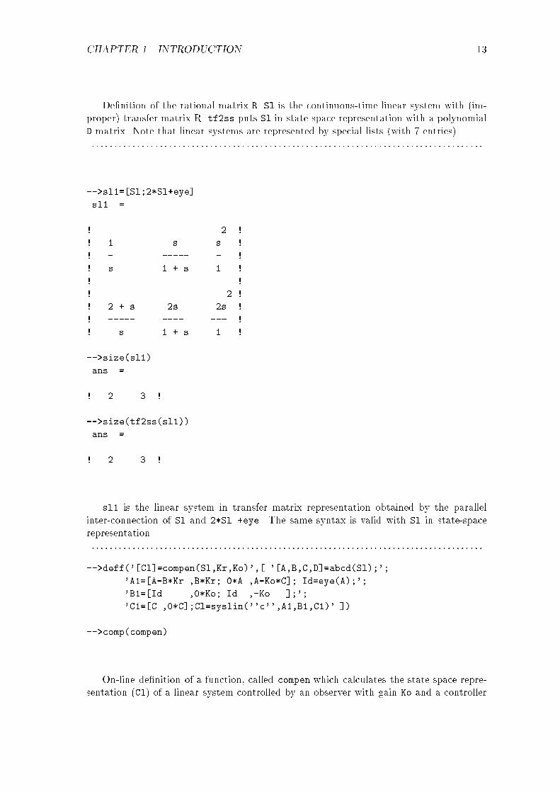
-->f21=f(2,1);v=0:0.01:%pi;frequencies=exp(%i*v);
-->response=freq(f21(2),f21(3),frequencies);
-->plot2d(v',abs(response)',[-1],'011',' ',[0,0,3.5,0.7],[5,4,5,7]);
-->xtitle(' ','radians','magnitude');

CHAPTER 1. INTRODUCTION 11
De�nition of a rational polynomial by extraction of an element of the matrix f de�nedabove. This is followed by the evaluation of the rational polynomial at the vector ofcomplex frequency values de�ned by frequencies. The evaluation of the polynomial isdone by the primitive freq. numer(f21) is the numerator polynomial and denom(f21)
is the denominator polynomial. The visualization of the resulting evaluation is made byusing the command plot2d (see Figure 1.1).. : : : : : : : : : : : : : : : : : : : : : : : : : : : : : : : : : : : : : : : : : : : : : : : : : : : : : : : : : : : : : : : : : : : : : : : : : : : : : : : : : : : : : : .
-->w=(1-s)/(1+s);f=1/p
f =
1
---------
2
1 + 2s + s
-->horner(f,w)
ans =
2
1 + 2s + s
----------
4
The function horner allows the user to make a (possibly symbolic) change of variablesfor a polynomial (for example, to perform the bilinear transformation as seen above).. : : : : : : : : : : : : : : : : : : : : : : : : : : : : : : : : : : : : : : : : : : : : : : : : : : : : : : : : : : : : : : : : : : : : : : : : : : : : : : : : : : : : : : .
-->A=[-1,0;1,2];B=[1,2;2,3];C=[1,0];
-->Sl=syslin('c',A,B,C);
-->ss2tf(Sl)
ans =
! 1 2 !
! ----- ----- !
! 1 + s 1 + s !
De�nition of a linear system in state-space representation. The function syslin de�neshere the continuous time ('c') system Sl with state-space matrices (A,B,C). The functionss2tf transforms Sl into transfer matrix representation.. : : : : : : : : : : : : : : : : : : : : : : : : : : : : : : : : : : : : : : : : : : : : : : : : : : : : : : : : : : : : : : : : : : : : : : : : : : : : : : : : : : : : : : .
CHAPTER 1. INTRODUCTION 12
-->s=poly(0,'s');
-->R=[1/s,s/(1+s),s^2]
R =
! 2 !
! 1 s s !
! - ----- - !
! s 1 + s 1 !
-->Sl=syslin('c',R);
-->tf2ss(Sl)
ans =
ans(1) (state-space system:)
lss
ans(2) = A matrix =
! - 0.5 - 0.5 !
! - 0.5 - 0.5 !
ans(3) = B matrix =
! - 0.7071068 0.7071068 0. !
! 0.7071068 0.7071068 0. !
ans(4) = C matrix =
! - 1.4142136 0. !
ans(5) = D matrix =
! 2 !
! 0 1 s !
ans(6) = X0 (initial state) =
! 0. !
! 0. !
ans(7) = Time domain =
c
CHAPTER 1. INTRODUCTION 13
De�nition of the rational matrix R. Sl is the continuous-time linear system with (im-proper) transfer matrix R. tf2ss puts Sl in state-space representation with a polynomialD matrix. Note that linear systems are represented by special lists (with 7 entries).. : : : : : : : : : : : : : : : : : : : : : : : : : : : : : : : : : : : : : : : : : : : : : : : : : : : : : : : : : : : : : : : : : : : : : : : : : : : : : : : : : : : : : : .
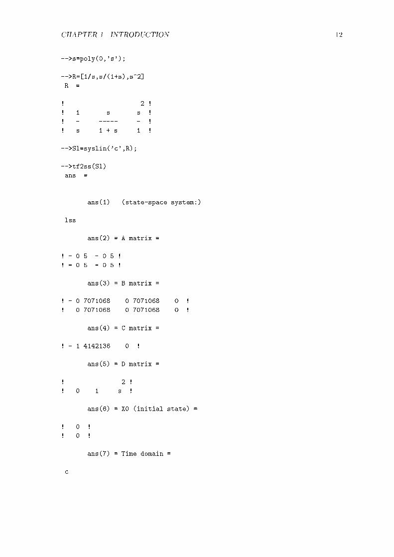
-->sl1=[Sl;2*Sl+eye]
sl1 =
! 2 !
! 1 s s !
! - ----- - !
! s 1 + s 1 !
! !
! 2 !
! 2 + s 2s 2s !
! ----- ---- --- !
! s 1 + s 1 !
-->size(sl1)
ans =
! 2. 3. !
-->size(tf2ss(sl1))
ans =
! 2. 3. !
sl1 is the linear system in transfer matrix representation obtained by the parallelinter-connection of Sl and 2*Sl +eye. The same syntax is valid with Sl in state-spacerepresentation.. : : : : : : : : : : : : : : : : : : : : : : : : : : : : : : : : : : : : : : : : : : : : : : : : : : : : : : : : : : : : : : : : : : : : : : : : : : : : : : : : : : : : : : .
-->deff('[Cl]=compen(Sl,Kr,Ko)',[ '[A,B,C,D]=abcd(Sl);';
'A1=[A-B*Kr ,B*Kr; 0*A ,A-Ko*C]; Id=eye(A);';
'B1=[Id ,0*Ko; Id ,-Ko ];';
'C1=[C ,0*C];Cl=syslin(''c'',A1,B1,C1)' ])
-->comp(compen)
On-line de�nition of a function, called compen which calculates the state space repre-sentation (Cl) of a linear system controlled by an observer with gain Ko and a controller

CHAPTER 1. INTRODUCTION 14
with gain Kr. Note that matrices are constructed in block form using other matrices. Thefunction compen is then compiled by comp.. : : : : : : : : : : : : : : : : : : : : : : : : : : : : : : : : : : : : : : : : : : : : : : : : : : : : : : : : : : : : : : : : : : : : : : : : : : : : : : : : : : : : : : .
-->A=[1,1 ;0,1];B=[0;1];C=[1,0];Sl=syslin('c',A,B,C);
-->Cl=compen(Sl,ppol(A,B,[-1,-1]),...
ppol(A',C',[-1+%i,-1-%i])');
-->f=Cl(2),spec(f)
f =
! 1. 1. 0. 0. !
! - 4. - 3. 4. 4. !
! 0. 0. - 3. 1. !
! 0. 0. - 5. 1. !
ans =
! - 1. !
! - 1. !
! - 1. + i !
! - 1. - i !
Call to the function compen de�ned above where the gains were calculated by a callto the primitive ppol which performs pole placement. The resulting f matrix is displayedand the placement of its poles is checked using the primitive spec which calculates theeigenvalues of a matrix. (The function compen is de�ned here on-line by deff as an exampleof function which receive a linear system (Sl) as input and returns a linear system (Cl)as output. In general Scilab functions are de�ned in �les and loaded in Scilab by getf).. : : : : : : : : : : : : : : : : : : : : : : : : : : : : : : : : : : : : : : : : : : : : : : : : : : : : : : : : : : : : : : : : : : : : : : : : : : : : : : : : : : : : : : .
-->//Saving the environment in a file named : myfile
-->save('myfile')
-->//Request to the host system to perform a system command
-->unix_s('rm myfile')
-->//Request to the host system with output in this Scilab window
-->unix_w('date')
Fri Mar 8 09:43:30 MET 1996
-->

CHAPTER 1. INTRODUCTION 15
Relation with the Unix environment and an error message: command is not inter-pretable by the system since the variable q is unknown.. : : : : : : : : : : : : : : : : : : : : : : : : : : : : : : : : : : : : : : : : : : : : : : : : : : : : : : : : : : : : : : : : : : : : : : : : : : : : : : : : : : : : : : .
-->foo=[' subroutine foo(a,b,c)';
' c=a+b';
' end' ];
-->unix_s('\rm foo.f')
-->write('foo.f',foo);
-->unix_s('make foo.o')
-->link('foo.o','foo')
-->deff('[c]=myplus(a,b)',...
'c=fort(''foo'',a,1,''r'',b,2,''r'',''out'',[1,1],3,''r'')')
-->myplus(5,7)
ans =
12.
De�nition of a column vector of character strings de�ning a Fortran subroutine. Theroutine is compiled (needs a compiler), dynamically linked to Scilab, and interactivelycalled by the function myplus.. : : : : : : : : : : : : : : : : : : : : : : : : : : : : : : : : : : : : : : : : : : : : : : : : : : : : : : : : : : : : : : : : : : : : : : : : : : : : : : : : : : : : : : .
-->deff('[ydot]=f(t,y)','ydot=[a-y(2)*y(2) -1;1 0]*y')
-->a=1;comp(f);y0=[1;0];t0=0;instants=0:0.02:20;
-->y=ode(y0,t0,instants,f);
-->plot2d(y(1,:)',y(2,:)',[-1],'011',' ',[-3,-3,3,3],[10,2,10,2])
-->xtitle('Van der Pol')
De�nition of a function which calculates a �rst order vector di�erential f(t,y). Thisis followed by the de�nition of the constant a used in the function and the function iscompiled. The primitive ode then integrates the di�erential equation de�ned by f(t,y)
for y(0) = h1; 0i at t = 0 and where the solution is given at the time values t =0; :02; :04; : : : ; 20. The result is plotted in Figure 1.2 where the �rst element of the in-tegrated vector is plotted against the second element of this vector.. : : : : : : : : : : : : : : : : : : : : : : : : : : : : : : : : : : : : : : : : : : : : : : : : : : : : : : : : : : : : : : : : : : : : : : : : : : : : : : : : : : : : : : .

CHAPTER 1. INTRODUCTION 16
-->m=['a' 'cos(b)';'sin(a)' 'c']
m =
!a cos(b) !
! !
!sin(a) c !
-->m*m'
!--error 43
not implemented in scilab....
-->deff('[x]=%cmc(a,b)',['[l,m]=size(a);[m,n]=size(b);x=[];';
'for j=1:n,y=[];';
'for i=1:l,t='' '';';
'for k=1:m;';
'if k>1 then t=t+''+(''+a(i,k)+'')*''+''(''+b(k,j)+'')'';';
'else t=''('' + a(i,k) + '')*'' + ''('' + b(k,j) + '')'';';
'end,end;';
'y=[y;t],end;';
'x=[x y],end,'])
-->m*m'
ans =
!(a)*(a)+(cos(b))*(cos(b)) (a)*(sin(a))+(cos(b))*(c) !
! !
!(sin(a))*(a)+(c)*(cos(b)) (sin(a))*(sin(a))+(c)*(c) !
De�nition of a matrix containing character strings. By default, the operation of sym-bolic multiplication of two matrices of character strings is not de�ned in Scilab. The(on-line) function de�nition for %cmc de�nes the multiplication of matrices of characterstrings (note that the double quote is necessary because the body of the deff containsquotes inside of quotes). The % which begins the function de�nition for %cmc allows thede�nition of an operation which did not previously exist in Scilab, and the name cmc
means \chain multiply chain". This example is not very useful: it is simply given to showhow operations can be de�ned on complex data structures.. : : : : : : : : : : : : : : : : : : : : : : : : : : : : : : : : : : : : : : : : : : : : : : : : : : : : : : : : : : : : : : : : : : : : : : : : : : : : : : : : : : : : : : .
-->deff('[y]=calcul(x,method)','z=method(x),y=poly(z,''x'')')
-->deff('[z]=meth1(x)','z=x')
-->deff('[z]=meth2(x)','z=2*x')
-->calcul([1,2,3],meth1)
ans =
CHAPTER 1. INTRODUCTION 17
2 3
- 6 + 11x - 6x + x
-->calcul([1,2,3],meth2)
ans =
2 3
- 48 + 44x - 12x + x
A simple example which illustrates the passing of a function as an argument to anotherfunction. Scilab functions are objects which may be de�ned, loaded, or manipulated asother objects such as matrices or lists.. : : : : : : : : : : : : : : : : : : : : : : : : : : : : : : : : : : : : : : : : : : : : : : : : : : : : : : : : : : : : : : : : : : : : : : : : : : : : : : : : : : : : : : .
-->quit
Exit from Scilab.. : : : : : : : : : : : : : : : : : : : : : : : : : : : : : : : : : : : : : : : : : : : : : : : : : : : : : : : : : : : : : : : : : : : : : : : : : : : : : : : : .
0.00 0.88 1.75 2.63 3.50
0.0
0.1
0.2
0.3
0.4
0.5
0.6
0.7magnitude
radians
Figure 1.1: A Simple Response

CHAPTER 1. INTRODUCTION 18
-3 0 3
-3
0
3
Van der Pol
Figure 1.2: Phase Plot

Chapter 2
Data Types
Scilab recognizes several primitive data types. Scalar objects are constants, booleans,polynomials, strings and rationals (quotients of polynomials). These objects in turn allowto de�ne matrices which admit these scalars as entries. Other basic objects are lists andfunctions. Only constant and boolean sparse matrices are de�ned. The objective of thischapter is to describe the use of each of these data types.
2.1 Special Constants
Scilab provides special constants %i, %pi, %e, and %eps as primitives. The %i constant rep-resents
p�1, %pi is � = 3:1415927 � � � , %e is the trigonometric constant e = 2:7182818 � � �,and %eps is a constant representing the precision of the machine (%eps is the biggestnumber for which 1+ %eps = 1). %inf and %nan stand for \in�nity" and \NotANumber"respectively.
Finally boolean constants are %t and %f which stand for \true" and \false" respectively.Note that %t is the same as 1==1 and %f is the same as ~%t.
These variables are considered as \prede�ned". They are protected, cannot be deletedand are not saved by the save command. It is possible for a user to have his own \pre-de�ned" variables by using the predef command. The best way is probably to set thesespecial variables in his own startup �le <home dir>/.scilab.
2.2 Constant Matrices
Scilab considers a number of data objects as matrices. Scalars, vectors, and matriceswhose entries are either real or complex are all considered as matrices. The details of theuse of these objects are revealed in the following Scilab sessions.
Scalars Scalars are either real or complex numbers. The values of scalars can be assignedto variable names chosen by the user.
--> a=5+2*%i
a =
5. + 2.i
--> B=-2+%i;
19

CHAPTER 2. DATA TYPES 20
--> b=4-3*%i
b =
4. - 3.i
--> a*b
ans =
26. - 7.i
-->a*B
ans =
- 12. + i
--> c=a+b;
-->c
c =
9. - i
Note that Scilab evaluates immediately lines that end with a carriage return. Instructionsthat end in a semi-colon are evaluated but are not displayed on screen. Scilab is casesensitive now (Version 2.0 was not case sensitive).
Vectors The usual way of creating vectors is as follows
--> v=[2,-3+%i,7]
v =
! 2. - 3. + i 7. !
--> v'
ans =
! 2. !
! - 3. - i !
! 7. !
--> w=[-3;-3-%i;2]
w =
! - 3. !
! - 3. - i !
! 2. !

CHAPTER 2. DATA TYPES 21
--> v'+w
ans =
! - 1. !
! - 6. - 2.i !
! 9. !
--> v*w
ans =
18.
--> w'.*v
ans =
! - 6. 8. - 6.i 14. !
Notice that vector elements that are separated by commas (or by blanks) yield row vectorsand those separated by semi-colons give column vectors. Note also that a single quote isused for transposing a vector (one obtains the complex conjugate for complex entries).Vectors of same dimension can be added and subtracted. The scalar product of a row andcolumn vector is demonstrated above. Element-wise multiplication (.*) and division (./)is also possible as was demonstrated.
Note with the following example the role of the position of the blank:
-->v=[1 +3]
v =
! 1. 3. !
-->w=[1 + 3]
w =
! 1. 3. !
-->w=[1+ 3]
w =
4.
-->u=[1, + 8- 7]
u =
! 1. 1. !
Vectors of elements which increase or decrease incrementely are constructed as follows

CHAPTER 2. DATA TYPES 22
--> v=5:-.5:3
v =
! 5. 4.5 4. 3.5 3. !
The resulting vector begins with the �rst value and ends with the third value steppingin increments of the second value. When not speci�ed the default increment is one. Aconstant vector can be created using the ones and zeros facility
--> v=[1 5 6]
v =
! 1. 5. 6. !
--> ones(v)
ans =
! 1. 1. 1. !
--> ones(v')
ans =
! 1. !
! 1. !
! 1. !
--> ones(1:4)
ans =
! 1. 1. 1. 1. !
--> 3*ones(1:4)
ans =
! 3. 3. 3. 3. !
-->zeros(v)
ans =
! 0. 0. 0. !
-->zeros(1:5)
ans =
! 0. 0. 0. 0. 0. !
Notice that ones or zeros replace its vector argument by a vector of equivalent dimensions�lled with ones or zeros.

CHAPTER 2. DATA TYPES 23
Matrices Row elements are separated by commas or spaces and column elements bysemi-colons. Multiplication of matrices by scalars, vectors, or other matrices is in theusual sense. Addition and subtraction of matrices is element-wise and element-wise mul-tiplication and division can be accomplished with the .* and ./ operators.
--> a=[2 1 4;5 -8 2]
a =
! 2. 1. 4. !
! 5. - 8. 2. !
--> b=ones(2,3)
b =
! 1. 1. 1. !
! 1. 1. 1. !
--> a.*b
ans =
! 2. 1. 4. !
! 5. - 8. 2. !
--> a*b'
ans =
! 7. 7. !
! - 1. - 1. !
Notice that the ones operator with two real numbers as arguments separated by a commacreates a matrix of ones using the arguments as dimensions (same for zeros). Matricescan be used as elements to larger matrices. Furthermore, the dimensions of a matrix canbe changed.
--> a=[1 2;3 4]
a =
! 1. 2. !
! 3. 4. !
--> b=[5 6;7 8]
b =
! 5. 6. !
! 7. 8. !
--> c=[9 10;11 12]
c =

CHAPTER 2. DATA TYPES 24
! 9. 10. !
! 11. 12. !
--> d=[a,b,c]
d =
! 1. 2. 5. 6. 9. 10. !
! 3. 4. 7. 8. 11. 12. !
--> e=matrix(d,3,4)
e =
! 1. 4. 6. 11. !
! 3. 5. 8. 10. !
! 2. 7. 9. 12. !
-->f=eye(e)
f =
! 1. 0. 0. 0. !
! 0. 1. 0. 0. !
! 0. 0. 1. 0. !
-->g=eye(4,3)
g =
! 1. 0. 0. !
! 0. 1. 0. !
! 0. 0. 1. !
! 0. 0. 0. !
Notice that matrix d is created by using other matrix elements. The matrix primitivecreates a new matrix e with the elements of the matrix d using the dimensions speci�edby the second two arguments. The element ordering in the matrix d is top to bottom andthen left to right which explains the ordering of the re-arranged matrix in e.
The function eye creates an m � n matrix with 1 along the main diagonal (if theargument is a matrix e , m and n are the dimensions of e ) .
Sparse constant matrices are de�ned through their nonzero entries (type help sparse
for more details). Once de�ned, they are manipulated as full matrices.
2.3 Matrices of Character Strings
Character strings can be created by using single quotes. Concatenation of strings isperformed by the + operation. Matrices of character strings are constructed as ordinarymatrices, e.g. using brackets. A very important feature of matrices of character stringsis the capacity to manipulate and create functions. Furthermore, symbolic manipulation

CHAPTER 2. DATA TYPES 25
of mathematical objects can be implemented using matrices of character strings. Thefollowing illustrates some of these features.
--> x=1;y=2;z=3;w=4;v=5;
--> a=['x' 'y';'z' 'w+v']
a =
!x y !
! !
!z w+v !
--> at=trianfml(a)
at =
!z w+v !
! !
!0 z*y-x*(w+v) !
--> evstr(at)
ans =
! 3. 9. !
! 0. - 3. !
Note that in the above Scilab session the function trianfml performs the symbolic trian-gularization of the matrix a. The value of the resulting symbolic matrix can be obtainedby using evstr.
A very important aspect of character strings is that they can be used to automaticallycreate new functions (for more on functions see Section 3.2). An example of automaticallycreating a function is illustrated in the following Scilab session where it is desired to studya polynomial of two variables s and t. Since polynomials in two independent variables arenot directly supported in Scilab, we can construct a new data structure using a list (seeSection 2.6). The polynomial to be studied is (t2 + 2t3)� (t+ t2)s+ ts2 + s3.
-->getf("macros/make_macro.sci");
-->s=poly(0,'s');
-->t=poly(0,'t');
-->p=list(t^2+2*t^3,-t-t^2,t,1+0*t);
-->pst=makefunction(p)
pst =
[p]=pst(t)
-->pst

CHAPTER 2. DATA TYPES 26
pst =
[p]=pst(t)
-->pst(1)
ans =
2 3
3 - 2s + s + s
Here the polynomial is represented by the command which puts the coe�cients of the vari-able s in the list p. The list p is then processed by the function makefunction which makesa new function pst. The contents of the new function can be displayed and this functioncan be evaluated at values of t. The creation of the new function pst is accomplished asfollows
function [newfunction]=makefunction(p)
n=size(p);
num=mulf(makestr(p(1)),'1');
for k=2:n,
new=mulf(makestr(p(k)),'s^'+string(k-1));
num=addf(num,new);
end,
text='p='+num;
deff('<p>=newfunction(t)',text),
function [str]=makestr(p)
n=degree(p)+1,
c=coeff(p),
str=string(c(1)),
x=part(varn(p),1),
xstar=x+'^',
for k=2:n,
ck=c(k),
if ck<>0 then,
str=addf(str,mulf(string(c(k)),(xstar+string(k-1))));
end;
end,
Here the function makefunction takes the list p and creates the function pst. Insideof makefunction there is a call to another function makestr which makes the string whichrepresents each term of the new two variable polynomial. The functions addf and mulf
are for adding and multiplying strings (i.e. addf(x,y) yields the string x+y). Finally, theessential command for creating the new function is the primitive deff. The deff primitivecreates a function de�ned by two matrices of character strings. Here the function p isde�ned by the two character strings '[p]=newfunction(t)' and text where the stringtext evaluates to the polynomial in two variables.

CHAPTER 2. DATA TYPES 27
2.4 Polynomials and Polynomial Matrices
Polynomials are easily created and manipulated in Scilab. Manipulation of polynomialmatrices is essentially identical to that of constant matrices. The poly primitive in Scilabcan be used to specify the coe�cients of a polynomial or the roots of a polynomial.
--> p=poly([1 2],'s')
p =
2
2 - 3s + s
--> q=poly([1 2],'s','c')
q =
1 + 2s
--> p+q
ans =
2
3 - s + s
--> p*q
ans =
2 3
2 + s - 5s + 2s
--> q/p
ans =
1 + 2s
-----------
2
2 - 3s + s
Note that the polynomial p has the roots 1 and 2 whereas the polynomial q has thecoe�cients 1 and 2. It is the third argument in the poly primitive which speci�es thecoe�cient ag option. In the case where the �rst argument of poly is a square matrixand the roots option is in e�ect the result is the characteristic polynomial of the matrix.
--> poly([1 2;3 4],'s')
ans =
2
- 2 - 5s + s
Polynomials can be added, subtracted, multiplied, and divided, as usual, but only betweenpolynomials of same formal variable.

CHAPTER 2. DATA TYPES 28
Polynomials, like real and complex constants, can be used as elements in matrices.This is a very useful feature of Scilab for systems theory.
--> s=poly(0,'s')
s =
s
--> a=[1 s;s 1+s^2]
a =
! 1 s !
! !
! 2 !
! s 1 + s !
--> b=[1/s 1/(1+s);1/(1+s) 1/s^2]
b =
! 1 1 !
! ------ ------ !
! s 1 + s !
! !
! 1 1 !
! --- --- !
! 2 !
! 1 + s s !
From the above examples it can be seen that matrices can be constructed from polynomialsand rationals.
2.5 Boolean Matrices
Boolean constants are %t and %f. They can be used in boolean matrices. The syntax isthe same as for ordinary matrices i.e. they can be concatenated, transposed, etc...
Operations symbols used with boolean matrices or used to create boolean matrices are== and ~.
If B is a matrix of booleans or(B) and and(B) perform the logical or and and.
-->%t
%t =
T
-->[1,2]==[1,3]
ans =

CHAPTER 2. DATA TYPES 29
! T F !
-->[1,2]==1
ans =
! T F !
-->a=1:5; a(a>2)
ans =
! 3. 4. 5. !
-->A=[%t,%f,%t,%f,%f,%f];
-->B=[%t,%f,%t,%f,%t,%t]
B =
! T F T F T T !
-->A|B
ans =
! T F T F T T !
-->A&B
ans =
! T F T F F F !
Sparse boolean matrices are generated when, e.g., two constant sparse matrices arecompared. These matrices are handled as ordinary boolean matrices.
2.6 Lists, Linear Systems
Scilab has a list data type. The list is a collection of data objects not necessarily of thesame type. A list can contain any of the already discussed data types as well as other lists,functions, and libraries. Lists are useful for de�ning structured data objects. For example,in Scilab linear systems are treated as lists. The basic function which is used for de�ninglinear systems is syslin. This function receives as parameters the constant matrices whichde�ne a linear system in state-space form or, in the case of system in transfer form itsinput must be a rational matrix. To be more speci�c, the calling sequence of syslin iseither Sl=syslin('dom',A,B,C,D,x0) or Sl=syslin('dom',trmat). dom is one of thecharacter strings 'c' or 'd' for continuous time or discrete time systems respectively. Itis useful to note that D can be a polynomial matrix (improper systems); D and x0 areoptional arguments. trmat is a rational matrix i.e. it is de�ned as a matrix of rationals(ratios of polynomials). Conversion from a representation to another is done by ss2tf ortf2ss. Improper systems are also treated.

CHAPTER 2. DATA TYPES 30
-->//list defining a linear system
-->A=[0 -1;1 -3];B=[0;1];C=[-1 0];
-->h=syslin('c',A,B,C)
h =
h(1) (state-space system:)
lss
h(2) = A matrix =
! 0. - 1. !
! 1. - 3. !
h(3) = B matrix =
! 0. !
! 1. !
h(4) = C matrix =
! - 1. 0. !
h(5) = D matrix =
0.
h(6) = X0 (initial state) =
! 0. !
! 0. !
h(7) = Time domain =
c
-->//conversion from state-space form to transfer form
-->hs=ss2tf(h)
hs =
1
---------
2
1 + 3s + s

CHAPTER 2. DATA TYPES 31
-->size(hs)
ans =
! 1. 1. !
-->hs(1)
ans =
r
-->hs(2)
ans =
1
-->hs(3)
ans =
2
1 + 3s + s
-->hs(4)
ans =
c
-->typeof(hs)
ans =
rational
-->//inversion of transfer matrix
-->inv(hs)
ans =
2
1 + 3s + s
----------
1
-->//inversion of state-space form
-->inv(h)
ans =
CHAPTER 2. DATA TYPES 32
ans(1) (state-space system:)
lss
ans(2) = A matrix =
[]
ans(3) = B matrix =
[]
ans(4) = C matrix =
[]
ans(5) = D matrix =
2
1 + 3s + s
ans(6) = X0 (initial state) =
[]
ans(7) = Time domain =
c
-->//conversion of this inverse
-->ss2tf(ans)
ans =
2
1 + 3s + s
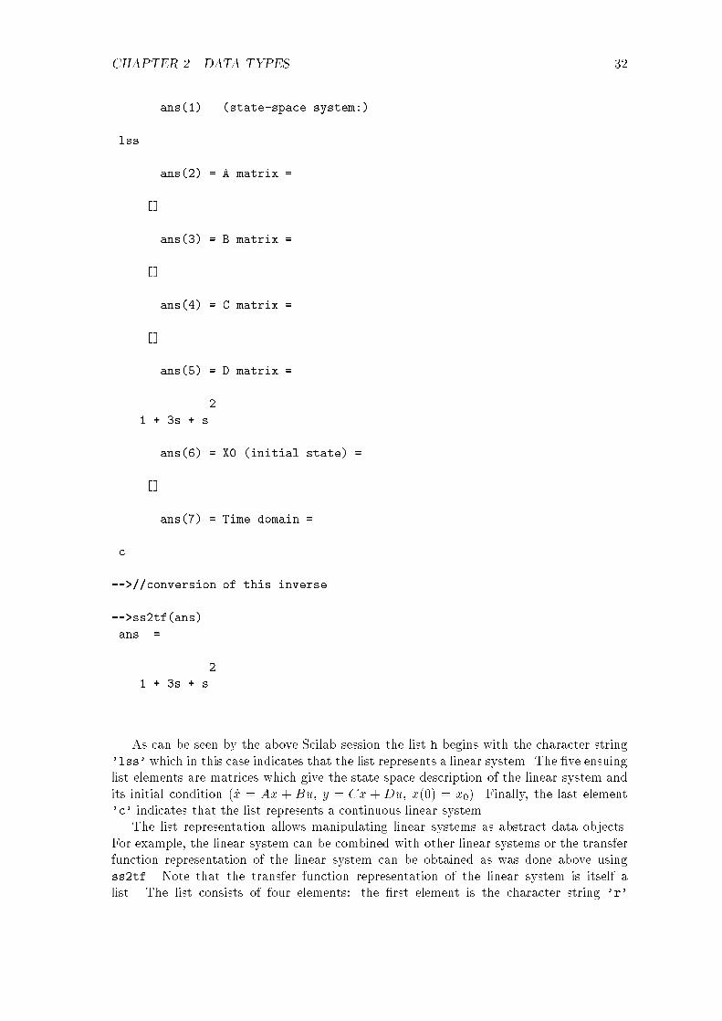
As can be seen by the above Scilab session the list h begins with the character string'lss' which in this case indicates that the list represents a linear system. The �ve ensuinglist elements are matrices which give the state space description of the linear system andits initial condition ( _x = Ax + Bu, y = Cx +Du, x(0) = x0). Finally, the last element'c' indicates that the list represents a continuous linear system.
The list representation allows manipulating linear systems as abstract data objects.For example, the linear system can be combined with other linear systems or the transferfunction representation of the linear system can be obtained as was done above usingss2tf. Note that the transfer function representation of the linear system is itself alist. The list consists of four elements: the �rst element is the character string 'r'

CHAPTER 2. DATA TYPES 33
s1*s2a - s1 - s2 - a
s1+s2a q
-
-
s2
s1?
6
i+ - a
[s1,s2]
a
a -
-
s2
s1?
6
i+ - a
[s1 ; s2]a q
-
-
s2
s1
-
-
a
a
s1/.s2
a -
s2
s1
�
a
Figure 2.1: Inter-Connection of Linear Systems
which indicates that the list represents a rational polynomial matrix, the second and thirdelements are the numerator and denominator polynomials, and �nally, the fourth elementis the character string 'c' which indicates that the transfer function is that of a continuoussystem. A very useful aspect of the manipulation of systems in Scilab is that a system canbe handled as a data object. Linear systems can be inter-connected, their representationcan easily be changed from state-space to transfer function and vice versa.
The inter-connection of linear systems can be made as illustrated in Figure 2.1. Foreach of the possible inter-connections of two systems s1 and s2 the command whichmakes the inter-connection is shown on the right side of the corresponding block diagramin Figure 2.1. Note that feedback interconnection is performed by s1/.s2.
The representation of linear systems can be in state-space form or in transfer functionform. These two representations can be interchanged by using the functions tf2ss andss2tf which change the representations of systems from transfer function to state-spaceand from state-space to transfer function, respectively. An example of the creation, thechange in representation, and the inter-connection of linear systems is demonstrated inthe following Scilab session.
-->//system connecting
-->s=poly(0,'s')

CHAPTER 2. DATA TYPES 34
s =
s
-->ft=1/(s-1)
ft =
1
-----
- 1 + s
-->gt=1/(s-2)
gt =
1
-----
- 2 + s
-->ft=syslin('c',ft);
-->gt=syslin('c',gt);
-->gls=tf2ss(gt);
-->ssprint(gls)
x = | 2 |x + | 1 |u
y = | 1 |x
-->hls=gls*ft;
-->ssprint(hls)
. | 2 1 | | 0 |
x = | 0 1 |x + | 1 |u
y = | 1 0 |x
-->ht=ss2tf(hls)
ht =
1
---------
2
2 - 3s + s
-->gt*ft

CHAPTER 2. DATA TYPES 35
ans =
1
---------
2
2 - 3s + s
The above session is a bit long but illustrates some very important aspects of thehandling of linear systems. First, two linear systems are created in transfer function formusing the primitive syslin. This primitive was used to label the systems in this exampleas being continuous (as opposed to being discrete). The primitive tf2ss is used to convertone of the two transfer functions to its equivalent state-space representation which is in listform (note that the function ssprint creates a more readable format for the state-spacelinear system). The following multiplication of the two systems yields their series inter-connection. Notice that the inter-connection of the two systems is e�ected even thoughone of the systems is in state-space form and the other is in transfer function form. Theresulting inter-connection is given in state-space form. Finally, the primitive ss2tf isused to convert the resulting inter-connected systems to the equivalent transfer functionrepresentation.
2.7 Functions (Macros)
Functions (also called macros) are a very useful aspect of Scilab. Functions are collectionsof commands which are executed in a new environment thus isolating function variablesfrom the original environments variables. Functions can be created and executed in anumber of di�erent ways. Furthermore, functions can pass arguments, have programmingfeatures such as conditionals and loops, and can be recursively called. Functions can bearguments to other functions and can be elements in lists. The most useful way of creatingfunctions is by using a text editor, however, functions can be created directly in the Scilabenvironment using the deff primitive.
--> deff('[x]=foo(y)','if y>0 then, x=1; else, x=-1; end')
--> foo(5)
ans =
1.
--> foo(-3)
ans =
- 1.
Usually functions are de�ned in a �le using an editor and loaded into Scilab with getf('filename')or getf('filename','c'). This can be done also by clicking in the File operation but-ton. This latter syntax loads the function(s) in filename and compiles them. The �rstline of filename must be as follows:

CHAPTER 2. DATA TYPES 36
function [y1,...,yn]=macname(x1,...,xk)
where the yi's are output variables and the xi's the input variables.For more on the use and creation of functions see Section 3.2.
2.8 Libraries
Libraries are collections of functions which can be either automatically loaded into theScilab environment when Scilab is called, or loaded when desired by the user. Librariesare created by the lib command. Examples of librairies are given in the SCIDIR/macrosdirectory. Note that in these directory there is an ASCII �le \names" which contains thenames of each function of the library, a set of .sci �les which contains the source codeof the functions and a set of .bin �les which contains the compiled code of the functions.The Make�le invokes scilab for compiling the functions and generating the .bin �les.The compiled functions of a library are automatically loaded into Scilab at their �rst call.
2.9 Objects
We conclude this chapter by noting that the function typeof returns the type of thevarious Scilab objects. The following objects are de�ned:
� usual for matrices with real or complex entries.
� polynomial for polynomial matrices: coe�cients can be real or complex.
� boolean for boolean matrices.
� character for matrices of character strings.
� uncompiled function for un-compiled functions.
� function for compiled functionds.
� rational for rational matrices (or linear systems in transfer matrix representation(syslin lists)
� state-space for linear systems in state-space form (syslin lists).
� sparse for sparse matrices.
� list for ordinary lists i.e. lists which do not represent linear systems (syslin lists).
� library for library de�nition.

Chapter 3
Programming
One of the most useful features of Scilab is its ability to create and use functions. Thisallows the development of specialized programs which can be integrated into the Scilabpackage in a simple and modular way through, for example, the use of libraries. In thischapter we treat the following subjects:
� Programming Tools
� De�ning and Using Functions
� De�nition of Operators for New Data Types
� Debbuging
Creation of libraries is discussed in a later chapter.
3.1 Programming Tools
Scilab supports a full list of programming tools including loops, conditionals, case selection,and creation of new environments. Most programming tasks should be accomplished inthe environment of a function. Here we explain what programming tools are available.
3.1.1 Comparison Operators
There exist �ve methods for making comparisons between the values of data objects inScilab. These comparisons are listed in the following table.
== or = equal to
< smaller than
> greater than
<= smaller or equal to
>= greater or equal to
<> or ~= not equal to
These comparison operators are used for evaluation of conditionals.
37

CHAPTER 3. PROGRAMMING 38
3.1.2 Loops
Two types of loops exist in Scilab: the for loop and the while loop. The for loop stepsthrough a vector of indices performing each time the commands delimited by end.
--> x=1;for k=1:4,x=x*k,end
x =
1.
x =
2.
x =
6.
x =
24.
The for loop can iterate on any vector or matrix taking for values the elements of thevector or the columns of the matrix.
--> x=1;for k=[-1 3 0],x=x+k,end
x =
0.
x =
3.
x =
3.
The for loop can also iterate on lists. The syntax is the same as for matrices.The while loop repeatedly performs a sequence of commands until a condition is
satis�ed.
--> x=1; while x<14,x=2*x,end
x =
2.
x =
4.
x =
8.
x =

CHAPTER 3. PROGRAMMING 39
16.
A for or while loop can be ended by the command break :
-->a=0;for i=1:5:100,a=a+1;if i > 10 then break,end; end
-->a
a =
3.
3.1.3 Conditionals
Two types of conditionals exist in Scilab: the if-then-else conditional and the select-case conditional. The if-then-else conditional evaluates an expression and if true exe-cutes the instructions between the then statement and the else statement (or end state-ment). If false the statements between the else and the end statement are executed.The else is not required. The elseif has the usual meaning and is a also a keywordrecognized by the interpreter.
--> x=1
x =
1.
--> if x>0 then,y=-x,else,y=x,end
y =
- 1.
--> x=-1
x =
- 1.
--> if x>0 then,y=-x,else,y=x,end
y =
- 1.
The select-case conditional compares an expression to several possible expressionsand performs the instructions following the �rst case which equals the initial expression.
--> x=-1
x =

CHAPTER 3. PROGRAMMING 40
- 1.
--> select x,case 1,y=x+5,case -1,y=sqrt(x),end
y =
i
It is possible to include an else statement for the condition where none of the cases aresatis�ed.
3.2 De�ning and Using Functions
It is possible to de�ne a function directly in the Scilab environment, however, the mostconvenient way is to create a �le containing the function with a text editor. In this sectionwe describe the structure of a function and several Scilab commands which are used almostexclusively in a function environment.
3.2.1 Function Structure
Function structure must obey the following format
function [y1,...,yn]=foo(x1,...,xm)
.
.
.
where foo is the function name, the xi are the m input arguments of the function, the yjare the n output arguments from the function, and the three vertical dots represent thelist of instructions performed by the function. An example of a function which calculatesk! is as follows
function [x]=fact(k)
k=int(k);
if k<1 then,
k=1;
end,
x=1;
for j=1:k,
x=x*j;
end,
If this function is contained in a �le called fact.sci the function is \loaded" into theScilab environment and is used as follows.
--> exists('fact')
ans =
0.
--> getf('../macros/fact.sci')

CHAPTER 3. PROGRAMMING 41
--> exists('fact')
ans =
1.
--> x=fact(5)
x =
120.
--> comp(fact)
In the above Scilab session, the command exists indicates that fact is not in the environ-ment (by the 0 answer to exist). The function is loaded into the environment using getf
and now exists indicates that the function is there (the 1 answer). The example calculates5!. Finally, the function is compiled using comp for faster execution. Note that compilingfact can be realized directly by the command getf('../macros/fact.sci','c').
3.2.2 Loading Functions
Functions are usually de�ned in �les. A �le which contains a function must obey thefollowing format
function [y1,...,yn]=foo(x1,...,xm)
.
.
.
where foo is the function name. The xi's are the input parameters and the the yj's arethe output parameters, and the three vertical dots represent the list of instructions per-formed by the function. Inputs and ouputs parameters can be any Scilab object (includingfunctions themeselves).
Functions are Scilab objects and should not be considered as �les. To be used in Scilab,functions de�ned in �les must be loaded by the command getf(filename,'c'). If the �lefilename contains the function foo, the function foo can be executed only if it has beenpreviously loaded by the command getf(filename,'c') (where 'c' is optional). A �lemay contain several functions. Functions can also be de�ned \on line" by the commanddeff. This is useful if one wants to de�ne a function as the output parameter of a otherfunction.
Collections of functions can be organized as libraries (see lib command). Stan-dard Scilab librairies (linear algebra, control,...) are de�ned in the subdirectories ofSCIDIR/macros/.
3.2.3 Global and Local Variables
If a variable in a function is not de�ned (and is not among the input parameters) thenit takes the value of a variable having the same name in the calling environment. Thisvariable however remains local in the sense that modifying it within the function does notalter the variable in the calling environment unless resume is used (see below). Functionscan be invoked with less input or output parameters. Here is an example:

CHAPTER 3. PROGRAMMING 42
function [y1,y2]=f(x1,x2)
y1=x1+x2
y2=x1-x2
-->[y1,y2]=f(1,1)
y2 =
0.
y1 =
2.
-->f(1,1)
ans =
2.
-->f(1)
y1=x1+x2;
!--error 4
undefined variable : x2
at line 2 of function f
-->x2=1;
-->[y1,y2]=f(1)
y2 =
0.
y1 =
2.
-->f(1)
ans =
2.
Note that it is not possible to call a function if one of the parameter of the callingsequence is not de�ned:
function [y]=f(x1,x2)
if x1<0 then y=x1, else y=x2;end
-->f(-1)
ans =
- 1.
-->f(-1,x2)

CHAPTER 3. PROGRAMMING 43
!--error 4
undefined variable : x2
-->f(1)
undefined variable : x2
at line 2 of function f called by :
f(1)
-->x2=3;f(1)
-->f(1)
ans =
3
3.2.4 Special Function Commands
Scilab has several special commands which are used almost exclusively in functions. Theseare the commands
� argn: returns the number of input and output arguments for the function
� error: used to suspend the operation of a function, to print an error message, andto return to the previous level of environment when an error is detected.
� warning,
� pause: temporarily suspends the operation of a function.
� break: forces the end of a loop
� return or resume : used to return to the calling environment and to pass localvariables from the function environment to the calling environment.
The following example loads a function called foo into Scilab which illustrates thesecommands.
-->getf('../macros/foo.sci')
-->foo
foo =
[z]=foo(x,y)
--> z=foo(0,1)
error('division by zero');
!--error 10000
division by zero
at line 4 of function foo called by :

CHAPTER 3. PROGRAMMING 44
z=foo(0,1)
--> z=foo(2,1)
-1-> resume
z =
0.7071068
--> s
s =
0.5
In the example we load foo.sci and display the contents of the function. The �rst callto foo passes an argument which cannot be used in the calculation of the function. Thefunction discontinues operation and indicates the nature of the error to the user. Thesecond call to the function suspends operation after the calculation of slope. Here theuser can examine values calculated inside of the function, perform plots, and, in factperform any operations allowed in Scilab. The -1-> prompt indicates that the currentenvironment created by the pause command is the environment of the function and notthat of the calling environment. Control is returned to the function by the commandreturn. Operation of the function can be stopped by the command quit or abort.Finally the function terminates its calculation returning the value of z. Also availablein the environment is the variable s which is a local variable from the function which ispassed to the global environment.
3.3 De�nition of Operations on New Data Types
It is possible to transparently de�ne fundamental operations for new data types in Scilab.That is, the user can give a sense to multiplication, division, addition, etc. on any two datatypes which exist in Scilab. As an example, two linear systems (represented by lists) canbe added together to represent their parallel inter-connection or can be multiplied togetherto represent their series inter-connection. Scilab performs these user de�ned operationsby searching for functions (written by the user) which follow a special naming conventiondescribed below.
The naming convention Scilab uses to recognize operators de�ned by the user is deter-mined by the following conventions. The name of the user de�ned function is composedof four (or possibly three) �elds. The �rst �eld is always the symbol %. The third �eld isone of the characters in the following table which represents the type of operation to beperformed between the two data types.

CHAPTER 3. PROGRAMMING 45
Third �eld
SYMBOL OPERATION
a +
b ; (row separator)
c [ ] (matrix de�nition)
d ./
e () extraction: m=a(k)
i () insertion: a(k)=m
k .*.
l \ left division
m *
p ^ exponent
q .\
r / right division
s -
t ' (transpose)
u *.
v /.
w \.
x .*
y ./.
z .\.
The second and fourth �elds represent the type of the �rst and second data objects,respectively, to be treated by the function and are represented by the symbols given inthe following table.
Second and Fourth �elds
SYMBOL VARIABLE TYPE
s scalar
p polynomial
l list (untyped)
c character string
m function
xxx list (typed)
A typed list is one in which the �rst entry of the list is a character string where the �rstthree characters of the string are represented by the xxx in the above table. For examplea list representing a linear system has the form list('lss',a,b,c,d,x0,'c') and, thus,the xxx above is lss.
An example of the function name which multiplies two linear systems together (torepresent their series inter-connection) is %lssmlss. Here the �rst �eld is %, the second�eld is lss (linear state-space), the third �eld is m \multiply" and the fourth one is lss.A possible user function which performs this multiplication is as follows
function [s]=%lssmlss(s1,s2)
[A1,B1,C1,D1,x1,dom1]=s1(2:7),
[A2,B2,C2,D2,x2]=s2(2:6),

CHAPTER 3. PROGRAMMING 46
B1C2=B1*C2,
s=list('lss',[A1,B1C2;0*B1C2' ,A2],...
[B1*D2;B2],[C1,D1*C2],D1*D2,[x1;x2],dom1),
An example of the use of this function after having loaded it into Scilab (using for examplegetf or inserting it in a library) is illustrated in the following Scilab session
-->A1=[1 2;3 4];B1=[1;1];C1=[0 1;1 0];
-->A2=[1 -1;0 1];B2=[1 0;2 1];C2=[1 1];D2=[1,1];
-->s1=syslin('c',A1,B1,C1);
-->s2=syslin('c',A2,B2,C2,D2);
-->ssprint(s1)
. | 1 2 | | 1 |
x = | 3 4 |x + | 1 |u
| 0 1 |
y = | 1 0 |x
-->ssprint(s2)
. | 1 -1 | | 1 0 |
x = | 0 1 |x + | 2 1 |u
y = | 1 1 |x + | 1 1 |u
-->s12=s1*s2; //This is equivalent to s12=%lssmlss(s1,s2)
-->ssprint(s12)
| 1 2 1 1 | | 1 1 |
. | 3 4 1 1 | | 1 1 |
x = | 0 0 1 -1 |x + | 1 0 |u
| 0 0 0 1 | | 2 1 |
| 0 1 0 0 |
y = | 1 0 0 0 |x
Notice that the use of %lssmss is totally transparent in that the multiplication of the twolists s1 and s2 is performed using the usual multiplication operator *.
The directory SCIDIR/macros/percent contains all the functions (a very large num-ber...) which perform operations on linear systems and transfer matrices. Conversions areautomatically performed. For example the code for the function %lssmlss is there (notethat it is much more complicated that the code given here!).

CHAPTER 3. PROGRAMMING 47
3.4 Debbuging
The simplest way to debug a Scilab function is to introduce a pause command in thefunction. When executed the function stops at this point and prompts -1-> which indi-cates a di�erent \level"; another pause gives -2-> ... At the level 1 the Scilab commandsare analog to a di�erent session but the user can display all the current variables presentin Scilab, which are inside or outside the function i.e. local in the function or belongingto the calling environment. The execution of the function is resumed by the commandreturn or resume (the variables used at the upper level are cleaned). The execution ofthe function can be interrupted by abort.
It is also possible to insert breakpoints in functions. See the commands setbpt,delbpt, disbpt. Finally, note that it is also possible to trap errors during the execu-tion of a function: see the commands errclear and errcatch. Finally the experts inScilab can use the function debug(i) where i=0,..,4 denotes a debugging level.

Chapter 4
Basic Primitives
This chapter brie y describes some basic primitives of Scilab. More detailed informationis given in the manual (see the directory SCIDIR/man/LaTex-doc).
4.1 The Environment and Input/Output
In this chapter we describe the most important aspects of the environment of Scilab: howto automatically perform certain operations when entering Scilab, and how to read andwrite data from and to the Scilab environment.
4.1.1 The Environment
Scilab is loaded with a number of variables and primitives. The command who lists thevariables which are available.
The who command also indicates how many elements and variables are available foruse. The user can obtain on-line help on any of the functions listed by typing help
<function-name>.Variables can be saved in an external binary �le using save. Similarly, variables
previously saved can be reloaded into Scilab using load.Note that after the command clear x y the variables x and y no longer exist in the
environment. The command save without any variable arguments saves the entire Scilabenvironment. Similarly, the command clear used without any arguments clears all of thevariables, functions, and libraries in the environment.
Functions which exist in �les can be seen by using disp and loaded by using getf.Libraries of functions are loaded using lib.The list of functions available in the library can be obtained by using disp.
4.1.2 Startup Commands by the User
When Scilab is called the user can automatically load into the environment functions, li-braries, variables, and perform commands using the the �le .scilab in his home directory.This is particularly useful when the user wants to run Scilab programs in the background(such as in batch mode). Another useful aspect of the .scilab �le is when some functionsor libraries are often used. In this case the command getf can be used in the .scilab
�le to automatically load the desired functions and libraries whenever Scilab is invoked.
48

CHAPTER 4. BASIC PRIMITIVES 49
4.1.3 Input and Output
Although the commands save and load are convenient, one has much more control overthe transfer of data between �les and Scilab by using the commands read and write.These two commands work similarly to the read and write commands found in Fortran.The syntax of these two commands is as follows.
--> x=[1 2 %pi;%e 3 4]
x =
! 1. 2. 3.1415927 !
! 2.7182818 3. 4. !
--> write('x.dat',x)
--> clear x
--> xnew=read('x.dat',2,3)
xnew =
! 1. 2. 3.1415927 !
! 2.7182818 3. 4. !
Notice that read speci�es the number of rows and columns of the matrix x. Complicatedformats can be speci�ed.
4.2 Help
On-line help is available either by clicking on the help button or by entering help item
(where item is usually the name of a function or primitive). The help facility is based onthe Unix xman command. apropos item looks for item in the whatis �le. This facilityis equivalent to the Unix whatis command. To add a new item in the manual is easy:just look at the SCIDIR/man subdirectories. The Scilab LaTEX manual is automaticallyobtained from the manual items by a Makefile. See the directory SCIDIR/man/Latex-doc.Note that the command manedit opens an help �le with an editor (default editor is emacs).
4.3 Nonlinear Calculation
Scilab has several powerful non-linear primitives for simulation or optimization.
4.3.1 Externals
An \external" is a function or Fortran routine which is used as an argument of some high-level primitives (such as ode, optim...). The calling sequence of the external (function orroutine) is imposed by the high-level primitive which sets the arguments of the external.For example the external function costfunc is an argument of the optim primitive. Itscalling sequence must be: [f,g,ind]=costfunc(x,ind) as imposed by the optim prim-itive. The following non-linear primitives in Scilab need externals: ode, optim, impl,

CHAPTER 4. BASIC PRIMITIVES 50
dassl, intg, fsolve. For problems where computation time is important, it is recom-mended to code the externals as Fortran subroutines. Examples of such subroutines aregiven in the directory SCIDIR/routines/default. When such a subroutine is written itmust be linked to Scilab. This link operation can be \dynamic" (see link). It is alsopossible to introduce the code in a more permanent manner by inserting it in a speci�cinterface (see e.g. fydot.f in SCIDIR/routines/default and rebuild a new Scilab by amake.
4.3.2 Nonlinear Primitives
The main simulation primitives in Scilab allow integrating a broad range of non-linearsystem functions of both explicit and implicit nature. It is also possible to integrate asystem of di�erential equations with a stopping time: integration is performed until thetrajectory reaches a given surface. In the following we illustrate the basic ode syntax forexample.
The example illustrates the basic usage of ode. Here we simulate the motion of a doublependulum. Let �1 and �2 be the angles that the �rst and second pendulum elements makewith the vertical and r1, r2, m1 and m2 be the lengths and masses of the respectivependulum elements. The non-linear di�erential equation which describes the motion ofthe pendulum is:"
mr1 m2r2 cos �r1 cos �1 r2
# "��1��2
#=
"�m2r2 _�
2
2sin �
r1 _�2
1sin �
#�"m sin �1sin �2
#g (4.1)
where g is the acceleration due to gravity, m = m1 +m2, and � = �1 + �2. The followingScilab session simulates the movement of the pendulum for 1:5 seconds where g = 9:8m=s,r1 = r2 = 1m, and m1 = m2 = 1kg. The initial conditions are �1 = �=2, �2 = �=2, _�1 = 0,and _�2 = 0.
--> m1=1;m2=1;r1=1;r2=1;
--> g=9.8;
--> t0=0;
--> t=0:.1:1.5;
--> z0=[%pi/2;%pi/2;0;0];
--> getf('../macros/dpend.sci','c');
--> z=ode(z0,t0,t,dpend);
--> pp(z)
The result of the above session is plotted in Figure 4.1. Note that ode takes four argu-ments: an initial condition vector z0, the initial time t0, a vector of times t for which theintegrated values z are desired, and the function dpend which exists in the environment ofScilab and which calculates the value of the derivative zd given the time t and the valueof z at this time.

CHAPTER 4. BASIC PRIMITIVES 51
-2.10 -0.70 0.70 2.10
-3.10
-1.70
-0.30
1.10
-2.10 -0.70 0.70 2.10
-3.10
-1.70
-0.30
1.10
-2.10 -0.70 0.70 2.10
-3.10
-1.70
-0.30
1.10
-2.10 -0.70 0.70 2.10
-3.10
-1.70
-0.30
1.10
-2.10 -0.70 0.70 2.10
-3.10
-1.70
-0.30
1.10
-2.10 -0.70 0.70 2.10
-3.10
-1.70
-0.30
1.10
-2.10 -0.70 0.70 2.10
-3.10
-1.70
-0.30
1.10
-2.10 -0.70 0.70 2.10
-3.10
-1.70
-0.30
1.10
-2.10 -0.70 0.70 2.10
-3.10
-1.70
-0.30
1.10
-2.10 -0.70 0.70 2.10
-3.10
-1.70
-0.30
1.10
-2.10 -0.70 0.70 2.10
-3.10
-1.70
-0.30
1.10
-2.10 -0.70 0.70 2.10
-3.10
-1.70
-0.30
1.10
-2.10 -0.70 0.70 2.10
-3.10
-1.70
-0.30
1.10
-2.10 -0.70 0.70 2.10
-3.10
-1.70
-0.30
1.10
-2.10 -0.70 0.70 2.10
-3.10
-1.70
-0.30
1.10
-2.10 -0.70 0.70 2.10
-3.10
-1.70
-0.30
1.10
Figure 4.1: Simulation of a Double Pendulum
Note that the dpend function calculates the derivative of the state of the double pen-dulum following (4.1).
function [zdot]=dpend(time,z)
th1=z(1);th2=z(2);th1d=z(3);th2d=z(4);
s12=sin(th1-th2);c12=cos(th1-th2);
m12=m1+m2;s1=sin(th1);s2=sin(th2);
mat=[m12*r1 m2*r2*c12;...
r1*c12 r2];
vec=-[m12*g*s1+m2*r2*th2d*th2d*s12;...
g*s2-r1*th1d*th1d*s12];
res=mat\vec;
th1dd=res(1);th2dd=res(2);
zdot=[th1d;th2d;th1dd;th2dd];
function []=pp(z)
th1=z(1,:);th2=z(2,:);
rc1=r1*cos(th1);rc2=r2*cos(th2);
rs1=r1*sin(th1);rs2=r2*sin(th2);
rs12=rs1+rs2;rc12=rc1+rc2;
rect=[-2.1,-3.1,2.1,1.1];
for k=1:maxi(size(th1));
plot2d([0 rs1(k) rs12(k)]',-[0 rc1(k) rc12(k)]',...
[-1],"011",' ',rect,[10,3,10,3]);
end,
The Scilab \external" function which calculates the derivative ( dpend in this example)must have a certain format. This format is as follows

CHAPTER 4. BASIC PRIMITIVES 52
function [xdot]=f(time,x)
.
.
.
The format speci�es that the argument list contain two variables. The �rst variable timeis a scalar which represents time, the second variable x is a vector (or matrix) of the statevalues. The returned value xdot is the calculated derivative and has the same dimensionsas x. For di�erential equations of order greater than one state augmentation is used.
The optimization primitive optim in Scilab is capable �nding locally optimum solutionsto a wide range of non-linear problems. In the following we illustrate the basic optim
syntax by example.The example used to illustrate the use of optim is the classic ray-tracing problem of
a plane wave travelling from one material to another. Here we pose the problem slightlydi�erently. Imagine a lifeguard on a beach and a person calling for help in the water.The lifeguard's speed on land is di�erent from his speed in water and, consequently, hewould like to choose the point along the border between beach and water which minimizesthe travel time to the calling person. This problem can be analytically solved when theborder between beach and water is a straight line. The problem may not be analyticallyresolvable when the function of the border is more complicated than a straight line.
The problem is posed as follows. Given that the lifeguard is at the origin of a Cartesiancoordinate system, that the person to be saved is at the coordinates (x; y), and thatthe border between the beach and the water can be described by the function d(x), thelifeguard's time of travel is
T (p) =
pp2 + d2(p)
vb+
p(x� p)2 + (y � d(p))2
vw(4.2)
where p is the x-axis coordinate of the point along the border through which the lifeguardpasses and where vs and vw are the respective speeds of the lifeguard on the beach and inthe water. Here we assume that the x coordinate given by p uniquely de�nes a point onthe border between the beach and the water.
We know that a locally optimum solution must make dT (p)=dt = 0 and we can calculatethe derivative of T as a function of the derivative of d
d
dtT (p) =
p+ ddp
vspp2 + d2
+(p� x) + (d� y)dp
vwp(x� p)2 + (y � d)2
(4.3)
where dp is the partial of d with respect to p. The following Scilab functions make thecalculations in (4.2) and (4.3).
function [t,t_p,ind]=swim(p,ind)
[d,d_p]=dpfun(p);
as=sqrt(d^2+p^2);
aw=sqrt((x-p)^2+(y-d)^2);
t=as/vs+aw/vw;
t_p=(p+d*d_p)/(vs*as)+((p-x)+(d-y)*d_p)/(vw*aw);
function [d,d_p]=dpfun(p);
d=1.75-exp(log(1.55)*p);
d_p=-log(1.55)*exp(log(1.55)*p);

CHAPTER 4. BASIC PRIMITIVES 53
where the functions d and dp are calculated by the function dpfun. These two functionsare used in the following Scilab session by the primitive optim to �nd the optimum pointp.
--> x=1;y=1;vs=5;vw=1;
--> getf('../macros/swim.sci');
--> getf('../macros/plotopt.sci');
--> [ts,ps,tps]=optim(swim,0)
end of optimization
tps =
4.580D-16
ps =
0.6144065
ts =
0.8303513
--> popt(ps);
Here it can be seen that the primitive optim takes two arguments and returns three values.The �rst argument is the name of the Scilab function which calculates the value of time(the cost) and the derivative of the time with respect to the value of p. The secondargument is a �rst guess for the value of p. The returned values are, respectively, theoptimal cost ts associated to the value of p which is the value in ps, and, �nally, the valueof the gradient at this point which is in tps.
The optimal path for the lifeguard is illustrated in Figure 4.2. The curved line rep-resents the shape of the shoreline and the dotted line represents the lifeguard's optimalpath.
4.4 Fortran or C Interface
Scilab can be easily interfaced with Fortran or C subroutines. The simplest way is usingthe dynamic link primitive link and the subroutine call primitive fort. Details are givenin the Scilab manual.
Fortran subprograms can also be linked to Scilab by using an external Fortran programcall interf. See the program interf.f in the directory SCIDIR/default where examplesare given.
These facilities are particularly useful for simulation and optimization of non-linearproblems or for introducing programs automatically generated by the computer algebrasystem Maple. There are two steps for interfacing dynamically a subroutine written inFortran with Scilab. These two steps are demonstrated in what follows.

CHAPTER 4. BASIC PRIMITIVES 54
0.0 0.2 0.4 0.6 0.8 1.0
0.0
0.2
0.4
0.6
0.8
1.0
Figure 4.2: Optimal Lifeguard Path
To link a fortran subroutine with Scilab it is �rst necessary to have a �le which containsthe executable object �le of the subroutine. We introduce the Fortran subroutine fibb
which calculates the nth Fibbonacci number fn (i.e. the sequence 0; 1; 1; 2; 3; 5; 8; : : :wherefn = fn�1 + fn�2).
subroutine fibb(fn,n)
n0=0
n1=1
if(n.ge.3)then
do 10 k=1,n-2
fn=n0+n1
n0=n1
n1=fn
10 continue
else
fn=n-1
endif
end
Assuming that the object �le for fibb is available in the �le fibb.o the following Scilabsession shows how to use the subroutine from Scilab.
-->unix("make fibb.o");
-->link('fibb.o','fibb')
-->link()
ans =

CHAPTER 4. BASIC PRIMITIVES 55
fibb
-->n=6
n =
6.
-->fn=fort('fibb',n,2,'i','out',[1,1],1,'r')
fn =
5.
The primitive link usually takes two arguments where the �rst argument is the name ofthe object �le and the second argument is the name of the subroutine call. Note that theprimitive c_link may be used to know all the previously linked subroutines. The use offort to call the subroutine fibb is a bit complicated. The arguments are divided into fourgroups. The �rst argument 'fibb' is the name of the called subroutine. The argument'out' divides the remaining arguments into two groups. The group of arguments between'fibb' and 'out' is the list of input arguments, their positions in the call to fibb, andtheir data type. The group of arguments to the right of 'out' are the dimensions of theoutput variables, their positions in the call to fibb, and their data type. The possible datatypes are real, integer, and double precision which are indicated, respectively, by the strings'r', 'i', and 'd'. The positions of the two arguments for fibb are n at position 2 andfn at positon 1 which explains the above call values. The vector [1,1] indicates that theoutput fn is a 1�1 matrix. The routines which are linked to Scilab can also access internalScilab variables (see the routine matz.f in the directory SCIDIR/routines/system2).
4.5 XWindow Dialog
It may be convenient to open a speci�c XWindow window for entering interactively pa-rameters inside a function or for a demo. This facility is possible thanks to e.g. thefunctions x_dialog, x_choose, x_mdialog, x_matrix and x_message. The demos whichcan be executed by clicking on the demo button provide simple examples of the use ofthese functions.
4.6 Maple Interface
The Maple procedure maple2scilab allows to numerically evaluate any Maple expressionin Scilab. On input this procedure takes a Maple matrix made of symbolic expressions.When maple2scilab is invoked in Maple, a Fortran program is automatically generated byMaple (via Macrofort package in Maple) together with a Scilab function which allows to(dynamically) call this subroutine. The parameters of the function are the Maple symbolsand thus the Maple matrix can be evaluated numerically in Scilab. The use of Fortran isfor speed purposes since the formal Maple expression can be extremely complicated.

CHAPTER 4. BASIC PRIMITIVES 56
Model Reg Proc
FF
Sensor
+U Y
UP
- - - -?
�
-
6
-
-ia a
a
q q q
Figure 4.3: Inter-Connected Systems
4.7 System Interconnection
The purpose of this section is to illustrate some of the more sophisticated aspects of Scilabby the way of an example. The example shows how Scilab can be used to symbolicallyrepresent the inter-connection of multiple systems which in turn can then be used tonumerically evaluate the performance of the inter-connected systems. The symbolic rep-resentation of the inter-connected systems is done with a function called bloc2exp andthe evaluation of the resulting system is done with evstr.
The example illustrates the symbolic inter-connection of the systems shown in Fig-ure 4.3. Figure 4.3 illustrates the classic regulator problem where the block labeled Proc
is to be controlled using feedback from the Sensor block and Reg block. The Reg blockcompares the output from the Model block to the output from the Sensor block to decidehow to regulate the Proc block. There is also a feed-forward block which �lters the inputsignal U to the Proc block. The outputs of the system are Y and UP.
The system illustrated in Figure 4.3 can be represented in Scilab by using the functionbloc2exp. The use of bloc2exp is illustrated in the following Scilab session. There atwo kinds of objects: \transfer" and \links". The example considered here admits 5transfers and 7 links. First the transfer are de�ned in a symbolic manner. Then linksare de�ned and an \interconnected system" is de�ned as a speci�c list. The functionbloc2exp evaluates symbolically the global transfer and evstr evaluates numerically theglobal transfer function once the systems are given \values", i.e. are de�ned as Scilablinear systems.
-->model=2;reg=3;proc=4;sensor=5;ff=6;somm=7;
-->tm=list('transfer','model');
-->tr=list('transfer',['reg(:,1)','reg(:,2)']);
CHAPTER 4. BASIC PRIMITIVES 57
-->tp=list('transfer','proc');
-->ts=list('transfer','sensor');
-->tf=list('transfer','ff');
-->tsum=list('transfer',['1','1']);
-->lum=list('link','input',[-1],[model,1],[ff,1]);
-->lmr=list('link','model output',[model,1],[reg,1]);
-->lrs=list('link','regulator output',[reg,1],[somm,1]);
-->lfs=list('link','feed-forward output',[ff,1],[somm,1]);
-->lsp=list('link','proc input',[somm,1],[proc,1],[-2]);
-->lpy=list('link','proc output',[proc,1],[sensor,1],[-1]);
-->lsup=list('link','sensor output',[sensor,1],[reg,2]);
-->syst=...
list('blocd',tm,tr,tp,ts,tf,tsum,lum,lmr,lrs,lfs,lsp,lpy,lsup);
-->[sysf,names]=bloc2exp(syst)
names =
names>1
input
names>2
!proc output !
! !
!proc input !
sysf =
!proc*((eye-reg(:,2)*sensor*proc)\(-(-ff-reg(:,1)*model))) !
! !
!(eye-reg(:,2)*sensor*proc)\(-(-ff-reg(:,1)*model)) !
Note that the argument to bloc2exp is a list of lists. The �rst element of the list systis (actually) the character string 'blocd' which indicates that the list represents a block-diagram inter-connection of systems. Each list entry in the list syst represents a blockor an inter-connection in Figure 4.3. The form of a list which represents a block begins

CHAPTER 4. BASIC PRIMITIVES 58
with a character string 'transfer' followed by a matrix of character strings which givesthe symbolic name of the block. If the block is multi-input multi-output the matrix ofcharacter strings must be represented as is illustrated by the block Reg.
The inter-connections between blocks is also represented by lists. The �rst element ofthe list is the character string 'link'. The second element of the inter-connection is itssymbolic name. The third element of the inter-connection is the input to the connection.The remaining elements are all the outputs of the connection. Each input and output toan inter-connection is a vector which contains as its �rst element the block number (forinstance the model block is assigned the number 2). The second element of the vectoris the port number for the block (for the case of multi-input multi-output blocks). If aninter-connection is not attached to anything the value of the block number is negative (asfor example the inter-connection labeled 'input' or is omitted.
The result of the bloc2exp function is a list of names which give the unassigned inputsand outputs of the system and the symbolic transfer function of the system given by sysf.The symbolic names in sysf can be associated to polynomials and evaluated using thefunction evstr. This is illustrated in the following Scilab session.
-->s=poly(0,'s');
-->ff=1;sensor=1;model=1;
-->proc=s/(s^2+3*s+2);
-->reg=[1/s 1/s];
-->sys=evstr(sysf)
sys =
! 1 + s !
! ---------- !
! 2 !
! 1 + 3s + s !
! !
! 2 3 !
! 2 + 5s + 4s + s !
! ---------------- !
! 2 3 !
! s + 3s + s !
The resulting polynomial transfer function links the input of the block system to the twooutputs. Note that the output of evstr is the rational polynomial matrix sys whereasthe output of bloc2exp is a matrix of character strings.
The symbolic evaluation which is given here is not very e�cient with large intercon-nected systems. The function bloc2ss performs the previous calculation in state-spaceformat. Each system is given now in state-space as a syslin list or simply as a gain (con-stant matrix). Note bloc2ss performs the necessary conversions if this is not done by theuser. Each system must be given a value before bloc2ss is called. All the calculations aremade in state-space representation even if the linear systems are given in transfer form.

CHAPTER 4. BASIC PRIMITIVES 59
4.8 Converting Scilab Functions to Fortran Routines
Scilab provides a compiler (under development) to transform some Scilab functions intoFortran subroutines. The routines which are thus obtained make use of the routines whichare in the Fortran libraries. All the basic matrix operations are available.
Let us consider the following Scilab function:
function [x]=macr(a,b,n)
z=n+m+n,
c(1,1)=z,
c(2,1)=z+1,
c(1,2)=2,
c(2,2)=0,
if n=1 then,
x=a+b+a,
else,
x=a+b-a'+b,
end,
y=a(3,z+1)-x(z,5),
x=2*x*x*2.21,
sel=1:5,
t=a*b,
for k=1:n,
z1=z*a(k+1,k)+3,
end,
t(sel,5)=a(2:4,7),
x=[a b;-b' a']
which can be translated into Fortran by using the function mac2for. Each input pa-rameter of the subroutine is described by a list which contains its type and its dimensions.Here, we have three input variables a,b,c which are, say, integer, double precision,
double precision with dimensions (m,m), (m,m), (1,1). This information is gatheredin the following list:
l=list();
l(1)=list('1','m','m');
l(2)=list('1','m','m');
l(3)=list('0','1','1');
The call to mac2for is made as follows:
comp(macr);
mac2for(macr2lst(macr),l)
The output of this command is a string containing a stand-alone Fortran subroutine.
subroutine macr(a,b,n,x,m,work,iwork)
c!
c automatic translation

CHAPTER 4. BASIC PRIMITIVES 60
.
.
.
double precision a(m,m),b(m,m),x(m+m,m+m),y,z1,24(m,m),work(*)
integer n,m,z,c(2,2),sel(5),k,iwork(*)
.
.
.
call dmcopy(b,m,x(1,m+1),m+m,m,m)
call dmcopy(work(iw1),m,x(m+1,1),m+m,m,m)
call dmcopy(work(iw1),m,x(m+1,m+1),m+m,m,m)
return
c
end
This routine can be linked to Scilab and interactively called.

Chapter 5
Graphics
This section introduces graphics in Scilab.
5.1 The Graphics Window
On the right side of the Delete button, a checker give the number wn of the graphicswindow. This number is given at the end of the title of the window, e.g. ScilabGraphic1.The button Raise (Create) Window raises the window wn if it exists and creates it if not.The button Set (Create) Window activates the window wn if it exists and simultaneouslycreates it if necessary. The Delete button closes the window wn if it exists. The executionof a plotting command automatically creates a window if necessary.
There are 4 buttons on the graphics window:
� 3D Rot.: for applying a rotation with the mouse to a 3D plot. This button isinhibited for a 2D plot.
� 2D Zoom: zooming on a 2D plot. This command can be recursively invoked. Thisbutton has no for a 3D plot.
� UnZoomx: return to the initial plot (not to the plot corresponding to the previouszoom in case of multiple zooms).
� File: this button opens di�erent commands and menus.
The �rst one is simple : Clear simply rubs out the plot of the window.
The next command Print... opens a selection panel for getting a paper output ofthe plot.
The Export command opens a panel selection for getting a copy of the plot on a �lewith a speci�ed format (Postscript, Latex).
The save command directly saves the plot on a �le with a speci�ed name. This �lecan be loaded later in Scilab for replotting.
The Delete is the same command (close) than the previous one but simply appliedto its window.
61

CHAPTER 5. GRAPHICS 62
5.2 The Media
There are di�erent graphics devices in Scilab which can be used to send graphics towindows or paper. The default is ScilabGraphic0 window .
The basic Scilab graphics commands are :
� driver: selects a graphic driver
� xinit: initializes a graphic driver
� xclear: clears one or more graphic windows
� xpause: a pause in milliseconds
� xselect: raises the current graphic window
� xclick: waits for a mouse click
� xend: closes a graphic session
The di�erent devices are:
� X11 : graphics device for the X11 window system
� Rec : an X Window driver (X11) which also records all the graphic commands. Thisis the default
� Wdp : an X11 driver without recorded graphics; the graphics are done on a pixmapand are send to the graphic window with the command xset("wshow"). The pixmapis cleared with the command xset("wwpc") or with the usual command xbasc()
� Pos : graphics device for Postscript printers
� Fig : graphics device for the X�g system
In fact, in many cases, one can ignore the existence of drivers and use the functionsxbasimp, xs2fig in order to send a graphic to a printer or in a �le for the Xfig system.For example with :
-->driver('Pos')
-->xinit('foo.ps')
-->plot(1:10)
-->xend()
-->driver('Rec')
-->plot(1:10)
-->xbasimp(0,'foo1.ps')

CHAPTER 5. GRAPHICS 63
we get two identical Postscript �les : 'foo.ps' and 'foo1.ps.0' (the appending 0 is thenumber of the active window where the plot has been done).
The default for plotting is the superposition; this can be avoided with the commandxbasc(window-number) which clears the recorded Scilab graphics command associatedwith the window window-number and clears this window (see the warning below for thedi�erence between xbasc and xclear).
If you enlarge a graphic window, the command xbasr(window-number) is executed byScilab. This command clears the graphic window window-number and replays the graphiccommands associated with it. One can call this function manually, in order to verify theassociated recorded graphics commands.
Any number of graphics windows can be created with buttons or with the commandsxset or xselect. The environment variable DISPLAY can be used to specify an X11Display or one can use the xinit function in order to open a graphic window on a speci�cdisplay.
5.3 2D Plotting
5.3.1 Basic 2D Plotting
The simplest 2D plot is plot(x,y) or plot(y): this is the plot of y as function of x wherex and y are 2 vectors; if x is missing, it is replaced by the vector (1,...,size(y)). If yis a matrix, its rows are plotted. There are optional arguments.
A �rst example is given by the following commands and the result is represented on�gure 5.1:
-->//first example of plotting
--> t=(0:0.05:1)';
--> ct=cos(2*%pi*t);
--> plot2d(t,ct)
The generic 2D multiple plot isplot2di(str,x,y,[style,strf,leg,rect,nax])
with i=missing,1,2,3,4.For the di�erent values of i we have:i=missing : piecewise linear plottingi=1 : as previous with possible logarithmic scalesi=2 : piecewise constant drawing stylei=3 : vertical barsi=4 : arrows style (e.g. ode in a phase space)-Parameter str : it is the string "abc" :str is empty if i is missing.a=e : means empty; the values of x are not used; (The user must give a dummy value
to x).a=o : means one; the x-values are the same for all the curves

CHAPTER 5. GRAPHICS 64
0.0 0.1 0.2 0.3 0.4 0.5 0.6 0.7 0.8 0.9 1.0
-1.0
-0.8
-0.6
-0.4
-0.2
0.0
0.2
0.4
0.6
0.8
1.0
Figure 5.1: First example of plotting
a=g : means general.b=l : a logarithmic scale is used on the X-axisc=l : a logarithmic scale is used on the Y-axis-Parameters x,y : two matrices of the same size [nl,nc] (nc is the number of curves
and nl is the number of points of each curve)-Parameter style : it is a real vector of size (1,nc); the style to use for curve j is
de�ned by size(j) (when only one curve is drawn style can specify the style and aposition to use for the caption).
-Parameter strf : it is a string of length 3 "xyz" corresponding to :x=1 : captions displayedy=1 : the argument rect is used to specify the boundaries of the plot.
rect=[xmin,ymin,xmax,ymax]
y=2 : the boundaries of the plot are computedy=0 : the current boundariesz=1 : an axis is drawnand the number of tics can be speci�ed by the nax argumentz=2 : the plot is only surrounded by a box-Parameter leg : it is the string of the captions for the di�erent plotted curves . This
string is composed of �elds separated by the @ symbol: for example ``module@phase''
(see example below). These strings are displayed under the plot with small segmentsrecalling the styles of the corresponding curves.
-Parameter rect : it is a vector of 4 values specifying the boundaries of the plotrect=[xmin,ymin,xmax,ymax].
For di�erent plots the simple commands without any argument show a demo (e.gplot2d3() ).
5.3.2 Specialized 2D Plottings
� champ : vector �eld in R2

CHAPTER 5. GRAPHICS 65
� fchamp : for a vector �eld in R2 de�ned by a function
� fplot2d : 2D plotting of a curve described by a function
� fgrayplot : gray level on a 2D plot
� errbar : creates a plot with error bars
5.3.3 Captions and Presentation
� xgrid : adds a grid on a 2D graphic
� xtitle : adds title and axis names on a 2D graphic
� titlepage : graphic title page
� plotframe : graphic frame with scaling and grid
The command plotframe is used to add a grid and graduations by choosing the numberof graduations and getting rounded numbers.
5.3.4 Plotting Some Geometric Figures
Polylines Plotting
� xsegs : draws a set of unconnected segments
� xrect : draws a single rectangle
� xfrect : �lls a single rectangle
� xrects : �lls or draws a set of rectangles
� xpoly : draws a polyline
� xpolys : draws a set of polylines
� xfpoly : �lls a polygon
� xfpolys : �lls a set of polygons
� xarrows : draws a set of unconnected arrows
� xfrect : �lls a single rectangle
� xclea : erases a rectangle on a graphic window
Curves Plotting
� xarc : draws an ellipsis
� xfarc : �lls an ellipsis
� xarcs : �lls or draws a set of ellipsis

CHAPTER 5. GRAPHICS 66
5.3.5 Writing by Plotting
� xstring : draws a string or a matrix of strings
� xstringl : computes a rectangle which surrounds a string
� xstringb : draws a string in a speci�ed box
� xnumb : draws a set of numbers
5.3.6 Manipulating the Plot and Graphics Context
Graphics Context
Some parameters of the graphics are controlled by a graphic context ( for example theline thickness) and others are controlled through graphics arguments. In the �rst example(Figure (5.1)), we use all the default arguments.
� xset : to set graphic context values. Some examples of the use of xset :
(i)-xset("use color",flag) changes to color or gray plot according to the values(1 or 0) of flag.
(ii)-xset("window",window-number) sets the current window to the window window-number
and creates the window if it doesn't exist.
(iii)-xset("wpos",x,y) �xes the position of the upper left point of the graphicwindow.
The choice of the font, the width and height of the window, the driver... can be doneby xset.
� xget : to get informations about the current graphic context. All the values of theparameters �xed by xset can be obtained by xget.
� xlfont : to load a new family of fonts from the XWindow Manager
Some Manipulations
Coordinates transforms :
� isoview : isometric scale without window change
allows an isometric scale in the window of previous plots without changing the win-dow size (see the example below).
� square : isometric scale with resizing the window
the window is resized according to the parameters of the command.
� scaling : scaling on data
� rotate : rotation
scaling and rotate executes respectively an a�ne transform and a geometric ro-tation of a 2-lines-matrix corresponding to the (x,y) values of a set of points.
� xgetech, xsetech : change of scale inside the graphic window
The current graphic scale can be �xed by a high level plot command. You may wantto get this parameter or to �x it directly : this is the role of xgetech, xsetech .

CHAPTER 5. GRAPHICS 67
5.4 Some Examples
We give here a sequence of commands corresponding to the di�erent capabilities of the2D plot and the generated �gures. This �rst example corresponds to the �gure 5.3.
x=-%pi:0.3:%pi;
y1=sin(x);y2=cos(x);y3=x;
X=[x;x;x]; Y=[y1;y2;y3];
plot2d2("g00",X',Y');
xbasc();
plot2d1("g00",X',Y',[1 2 3]',"101","caption1@caption2@caption3");
xtitle(["General";"Title"],"x-axis title","y-axis title");
xgrid([10,20]);
xclea(0.5,-0.5,1.5,1.5);
titlepage("titlepage");
xstring(0.65,0.3,["xstring after";"xclear"],0,1);
-3.14 -2.54 -1.94 -1.34 -0.74 -0.14 0.46 1.06 1.66 2.26 2.86
-3.14
-2.54
-1.94
-1.34
-0.74
-0.14
0.46
1.06
1.66
2.26
2.86
Figure 5.2: Simple 2D Plot
We give now the sequence of the commands for obtaining the �gure 5.5.
// initialize default environment variables
plot(1:10)
xbasc()
// simple rectangle
xrect(0,1,3,1)
// filling a rectangle
xfrect(3.1,1,3,1)
// writing in the rectangle

CHAPTER 5. GRAPHICS 68
-3.14 -2.54 -1.94 -1.34 -0.74 -0.14 0.46 1.06 1.66 2.26 2.86
-3.14
-2.54
-1.94
-1.34
-0.74
-0.14
0.46
1.06
1.66
2.26
2.86
+
+
++
+ + ++
+
+
+
+
+
++
+ + ++
+
+
× ××
×
×
×
×
××
× × × ××
×
×
×
×
××
×
⊕
⊕
⊕
⊕
⊕
⊕
⊕
⊕
⊕
⊕
⊕
⊕
⊕
⊕
⊕
⊕
⊕
⊕
⊕
⊕
⊕
caption1+caption2×caption3⊕
y-axis title
x-axis title
General
Title
titlepage
xclear
xstring after
Figure 5.3: Some Capabilities of 2D Plot
-5 0 5 10 15 20 25 30
0.0
0.5
1.0y
x
Plot with grid and automatic bounds
Figure 5.4: Use of plotframe

CHAPTER 5. GRAPHICS 69
xstring(0.5,0.5,"xrect(0,1,3,1)")
// writing black on black !
xstring(4.,0.5,"xfrect(3.1,1,3,1)")
// reversing the video
xset("alufunction",6)
xstring(4.,0.5,"xfrect(3.1,1,3,1)")
xset("alufunction",3)
// drawing a polyline
xv=[0 1 2 3 4]
yv=[2.5 1.5 1.8 1.3 2.5]
xpoly(xv,yv,"lines",1)
xstring(0.5,2.,"xpoly(xv,yv,""lines"",1)")
// drawing arrows
xa=[5 6 6 7 7 8 8 9 9 5]
ya=[2.5 1.5 1.5 1.8 1.8 1.3 1.3 2.5 2.5 2.5]
xarrows(xa,ya)
xstring(5.5,2.,"xarrows(xa,ya)")
// drawing a part of an ellipsis
xarc(0.,5.,4.,2.,0.,64*300.)
xstring(0.5,4,"xarc(0.,5.,4.,2.,0.,64*300.)")
xfarc(5.,5.,4.,2.,0.,64*360.)
xset("alufunction",6)
xstring(5.5,4.,"xfarc(5.,5.,4.,2.,0.,64*360.)")
xset("alufunction",3)
// writing a string
xstring(0.,4.5,"WRITING-BY-XSTRING()",-22.5)
5.5 3D Plotting
5.5.1 Generic 3D Plotting
� plot3d : 3D plotting of a matrix of points : plot3d(x,y,z) with x,y,z 3 matrices, zbeing the values for the points with coordinates x,y. Other arguments are optional
� plot3d1 : 3d plotting of a matrix of points with gray levels
� fplot3d : 3d plotting of a surface described by a function; z is given by an externalz=f(x,y)
� fplot3d1 : 3d plotting of a surface described by a function with gray levels
5.5.2 Specialized 3D Plotting
� param3d : plots parametric curves in 3d space
� contour : level curves for a 3d function given by a matrix
� grayplot10 : gray level on a 2d plot

CHAPTER 5. GRAPHICS 70
xrect(0,1,3,1) xfrect(3.1,1,3,1) xfrect(3.1,1,3,1)
xpoly(xv,yv,"lines",1) xarrows(xa,ya)
xarc(0.,5.,4.,2.,0.,64*300.) xfarc(5.,5.,4.,2.,0.,64*360.)
WRITING-BY-XSTRING() 3 14 15
isoview + xarc
Figure 5.5: Geometric Graphics and Comments
� fcontour10 : level curves for a 3d function given by a function
� hist3d : 3d histogram
� secto3d : conversion of a surface description from sector to plot3d compatible data
� eval3d : evaluates a function on a regular grid. (see also feval)
5.5.3 Mixing 2D and 3D graphics
When one uses 3D plotting function, default graphic boundaries are �xed, but in R3.If one wants to use graphic primitives to add informations on 3D graphics, the geom3d
function can be used to convert 3D coordinates to 2D-graphics coordinates. The �gure 5.6illustrates this feature.
xinit('d7-10.ps');
r=(%pi):-0.01:0;x=r.*cos(10*r);y=r.*sin(10*r);
deff("[z]=surf(x,y)","z=sin(x)*cos(y)");
t=%pi*(-10:10)/10;
fplot3d(t,t,surf,35,45,"X@Y@Z",[-1,2,3]);
z=sin(x).*cos(y);
[x1,y1]=geom3d(x,y,z);
xpoly(x1,y1,"lines");
[x1,y1]=geom3d([0,0],[0,0],[5,0]);
xsegs(x1,y1);
xstring(x1(1),y1(1),' The point (0,0,0)');

CHAPTER 5. GRAPHICS 71
Z
Y
X
The point (0,0,0)
Figure 5.6: 2D and 3D plot
5.5.4 Sub-windows
It is also possible to make multiple plotting in the same graphic window (Figure 5.7).
xinit('d7-8.ps');
t=(0:.05:1)';st=sin(2*%pi*t);
xsetech([0,0,1,0.5]);
plot2d2("onn",t,st);
xsetech([0,0.5,1,0.5]);
plot2d3("onn",t,st);
xsetech([0,0,1,1]);
5.5.5 A Set of Figures
In this next example we give a brief summary of di�erent plotting functions for 2D or 3Dgraphics. The �gure 5.8 is obtained and inserted in this document with the help of thecommand Blatexprs.
//some examples
str_l=list();
//
str_l(1)=['plot3d1();';
'title=[''plot3d1 : z=sin(x)*cos(y)''];';
'xtitle(title,'' '','' '');'];
//
str_l(2)=['contour();';
'title=[''contour ''];';
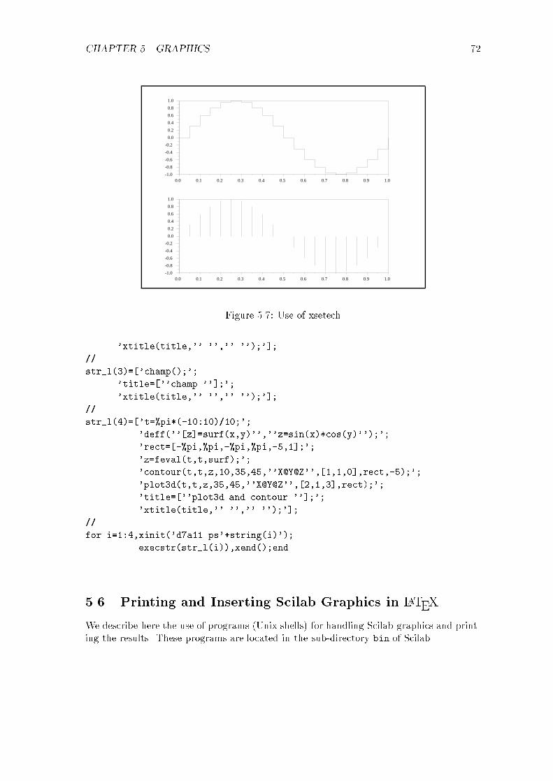
CHAPTER 5. GRAPHICS 72
0.0 0.1 0.2 0.3 0.4 0.5 0.6 0.7 0.8 0.9 1.0-1.0
-0.8
-0.6
-0.4
-0.2
0.0
0.2
0.4
0.6
0.8
1.0
0.0 0.1 0.2 0.3 0.4 0.5 0.6 0.7 0.8 0.9 1.0-1.0
-0.8
-0.6
-0.4
-0.2
0.0
0.2
0.4
0.6
0.8
1.0
Figure 5.7: Use of xsetech
'xtitle(title,'' '','' '');'];
//
str_l(3)=['champ();';
'title=[''champ ''];';
'xtitle(title,'' '','' '');'];
//
str_l(4)=['t=%pi*(-10:10)/10;';
'deff(''[z]=surf(x,y)'',''z=sin(x)*cos(y)'');';
'rect=[-%pi,%pi,-%pi,%pi,-5,1];';
'z=feval(t,t,surf);';
'contour(t,t,z,10,35,45,''X@Y@Z'',[1,1,0],rect,-5);';
'plot3d(t,t,z,35,45,''X@Y@Z'',[2,1,3],rect);';
'title=[''plot3d and contour ''];';
'xtitle(title,'' '','' '');'];
//
for i=1:4,xinit('d7a11.ps'+string(i)');
execstr(str_l(i)),xend();end
5.6 Printing and Inserting Scilab Graphics in LaTEX
We describe here the use of programs (Unix shells) for handling Scilab graphics and print-ing the results. These programs are located in the sub-directory bin of Scilab.

CHAPTER 5. GRAPHICS 73
1
0
-1
Z
-3.14
-0.14
2.86
Y
2.86
-0.14
-3.14
X
plot3d1 : z=sin(x)*cos(y)
1.0 1.4 1.8 2.2 2.6 3.0 3.4 3.8 4.2 4.6 5.0
1.0
1.9
2.8
3.7
4.6
5.5
6.4
7.3
8.2
9.1
10.0
0.19
0.19
0.19
0.190.37
0.37
0.37
0.37
0.37
0.37
0.37
0.37
0.37
0.56
0.56
0.56
0.56
0.56
0.56
0.56
0.56
0.56
0.56
0.75
0.75
0.75
0.75
0.75
0.75
0.75
contour
1.0 1.9 2.8 3.7 4.6 5.5 6.4 7.3 8.2 9.1 10.0
1.0
1.9
2.8
3.7
4.6
5.5
6.4
7.3
8.2
9.1
10.0
champ
-0.8
-0.8-0.8
-0.6
-0.6-0.6
-0.4
-0.4 -0.4
-0.2
-0.2 -0.20.0
0.0
0.0 0.2
0.2
0.2
0.4
0.4
0.4
0.6
0.6
0.6
0.8
0.8
0.8
Z
YX
plot3d and contour
Figure 5.8: Group of �gures

CHAPTER 5. GRAPHICS 74
5.6.1 Window to Paper
The simplest command to get a paper copy of a plot is to click on the print button ofthe ScilabGraphic window.
5.6.2 Creating a Postscript File
We have seen at the beginning of this chapter that the simplest way to get a Postscript�le containing a Scilab plot is :
-->driver('Pos')
-->xinit('foo.ps')
-->plot3d1();
-->xend()
-->driver('Rec')
-->plot3d1()
-->xbasimp(0,'foo1.ps')
The Postscript �les (foo.ps or foo1.ps ) generated by Scilab cannot be directly sentto a Postscript printer, they need a preamble. Therefore, printing is done through the useof Unix scripts or programs which are provided with Scilab. The program Blpr is used toprint a set of Scilab Graphics on a single sheet of paper and is used as follows :
Blpr string-title file1.ps file2.ps > result
You can then print the �le result with the classical Unix command :
lpr -Pprinter-name result
or use the ghostview Postscript interpreter on your Unix workstation to see the result.You can avoid the �le result with a pipe, replacing > result by the printing command
| lpr or the previewing command | ghostview -.The best result (best sized �gures) is obtained when printing two pictures on a single
page.
5.6.3 Including a Postscript File in LaTEX
The Blatexpr Unix shell and the programs Batexpr2 and Blatexprs are provided inorder to help inserting Scilab graphics in LaTEX.
Taking the previous �le foo.ps and typing the following statement under a Unix shell :
Blatexpr 1.0 1.0 foo.ps
creates two �les foo.epsf and foo.tex. The original Postscript �le is left unchanged. Toinclude the �gure in a LaTEX document you should insert the following LaTEX code inyour LaTEX document :

CHAPTER 5. GRAPHICS 75
\input foo.tex
\dessin{The caption of your picture}{The-label}
You can also see your �gure by using the Postscript previewer ghostview.The program Blatexprs does the same thing: it is used to insert a set of Postscript
�gures in one LaTEXpicture.In the following example, we begin by using the Postscript driver Pos and then initialize
successively 4 Postscript �les fig1.ps, ..., fig4.ps for 4 di�erent plots and at the endreturn to the driver Rec (X11 driver with record).
-->//multiple Postscript files for Latex
-->driver('Pos')
-->
-->t=%pi*(-10:10)/10;
-->
-->plot3d1(t,t,sin(t)'*cos(t),35,45,'X@Y@Z',[2,2,4]);
-->xend()
-->
-->contour(1:5,1:10,rand(5,10),5);
-->xend()
-->
-->champ(1:10,1:10,rand(10,10),rand(10,10));
-->xend()
-->
-->t=%pi*(-10:10)/10;
-->deff('[z]=surf(x,y)','z=sin(x)*cos(y)');
-->rect=[-%pi,%pi,-%pi,%pi,-5,1];
-->z=feval(t,t,surf);
-->contour(t,t,z,10,35,45,'X@Y@Z',[1,1,0],rect,-5);
-->plot3d(t,t,z,35,45,'X@Y@Z',[2,1,3],rect);

CHAPTER 5. GRAPHICS 76
0.0 1.9 3.8 5.6 7.5 9.4 11.3 13.2 15.0 16.9 18.8
-1.0
-0.8
-0.6
-0.4
-0.2
-0.0
0.2
0.4
0.6
0.8
1.0
plot2d and xgrid
t
sin(t)
-6 -5 -4 -3 -2 -1 0 1 2 3 4 5 6
0.0
0.1
0.2
0.3
0.4
0.5
0.6
0.7
0.8
0.9
1.0
1.1
macro histplot : Histogram plot
Classes
N(C)/Nmax
Figure 5.9: Blatexp2 Example
-->title=['plot3d and contour '];
-->xtitle(title,' ',' ');
-->xend()
-->
-->driver('Rec')
Then we execute the command :
Blatexprs multi fig1.ps fig2.ps fig3.ps fig4.ps
and we get 2 �les multi.tex and multi.ps and you can include the result in a LaTEX source�le by :
\input multi.tex
\dessin{The caption of your picture}{The-label}
Note that the second line dessin... is absolutely necessary and you have of course togive the absolute path for the input �le if you are working in another directory (see below).The �le multi.tex is only the de�nition of the command dessin with 2 parameters : thecaption and the label; the command dessin can be used with one or two empty arguments`` `` if you want to avoid the caption or the label.
The Postscipt �les are inserted in LaTEX with the help of the \special command andwith a syntax that works with the dvips program.
The program Blatexpr2 is used when you want two pictures side by side.
Blatexpr2 Fileres file1.ps file2.ps
It is sometimes convenient to have a main LaTEX document in a directory and tostore all the �gures in a subdirectory. The proper way to insert a picture �le in the maindocument, when the picture is stored in the subdirectory figures, is the following :

CHAPTER 5. GRAPHICS 77
\def\Figdir{figures/} % My figures are in the {\tt figures/ } subdirectory.
\input{\Figdir fig.tex}
\dessin{The caption of you picture}{The-label}
The declaration \def\Figdir{figures/} is used twice, �rst to �nd the �le fig.tex
(when you use latex), and second to produce a correct pathname for the special
LaTEX command found in fig.tex. (used at dvips level).-WARNING : the default driver is Rec, i.e. all the graphic commands are recorded,
one record corresponding to one window. The xbasc() command erases the plot on theactive window and all the records corresponding to this window. The clear button hasthe same e�ect; the xclear command erases the plot but the record is preserved. So youalmost never need to use the xbasc() or clear commands. If you use such a commandand if you re-do a plot you may have a surprising result (if you forget that the environmentis wiped out); the scale only is preserved and so you may have the \window-plot" and the\paper-plot" completely di�erent.
5.6.4 Postscript by Using X�g
Another useful way to get a Postscript �le for a plot is to use X�g. By the simple commandxs2fig(active-window-number,file-name) you get a �le in X�g syntax.
This command needs the use of the driver Rec.The window ScilabGraphic0 being active, if you enter :
-->t=-%pi:0.3:%pi;
-->plot3d1(t,t,sin(t)'*cos(t),35,45,'X@Y@Z',[2,2,4]);
-->xs2fig(0,'demo.fig');
you get the �le demo.fig which contains the plot of window 0.Then you can use X�g and after the modi�cations you want, get a Postscript �le that
you can insert in a LaTEX �le. The following �gure is the result of X�g after adding somecomments.
5.6.5 Encapsulated Postscript Files
As it was said before, the use of Blatexpr creates 2 �les : a .tex �le to be inserted in theLaTEX �le and a .epsf �le.
It is possible to get the encapsulated Postscript �le corresponding to a .ps �le by usingthe command BEpsf.
Notice that the .epsf �le generated by Blatexpr is not an encapsulated Postscript�le : it has no bounding box and BEpsf generates a .eps �le which is an encapsulatedPostscript �le with a bounding box.

CHAPTER 5. GRAPHICS 78
POSTSCRIPT USING XFIG
1
0
-1
Z
-3
-0
3
Y
3
-0
-3
X
40 DEGRES
LOCAL MAX
Figure 5.10: Encapsulated Postscript by Using X�g

Chapter 6
Maple to Scilab Interface
To combine symbolic computation of the computer algebra system Maple with the numer-ical facilities of Scilab, Maple objects can be transformed into Scilab functions. To assuree�cient numerical evaluation this is done through numerical evaluation in Fortran. Thewhole process is done by a Maple procedure called maple2scilab.
6.1 Maple2scilab
The procedure maple2scilab converts a Maple object, either a scalar function or a ma-trix into a Fortran subroutine and writes the associated Scilab function. The code ofmaple2scilab is in the directory SCIDIR/maple.
The calling sequence of maple2scilab is as follows:maple2scilab(function-name,object,args)
� The �rst argument, function-name is a name indicating the function-name in Scilab.
� The second argument object is the Maple name of the expression to be transferredto Scilab.
� The third argument is a list of arguments containing the formal parameters of theMaple-object object.
When maple2scilab is invoked in Maple, two �les are generated, one which containsthe Fortran code and another which contains the associated Scilab function. Aside theirexistence, the user has not to know about their contents.
The Fortran routine which is generated has the following calling sequence:<Scilab-name>(x1,x2,: : :,xn,matrix)
and this subroutine computes matrix(i,j) as a function of the arguments x1,x2,: : :,xn.Each argument can be a Maple scalar or array which should be in the argument list. TheFortran subroutine is put into a �le named <Scilab-name>.f, the Scilab-function into a�le named <Scilab-name>.sci. For numerical evaluation in Scilab the user has to compilethe Fortran subroutine, to link it with Scilab (e.g. Menu-bar option 'link') and to loadthe associated function (Menu-bar option 'getfc'). Information about link operation isgiven in Scilab's manual: Fortran routines can be incorporated into Scilab by dynamic linkor through the interf.f �le in the default directory. Of course, this two-step procedurecan be automatized using a shell-script (or using unix in Scilab). Maple2scilab uses the\Macrofort" library which is in the share library of Maple.
79
CHAPTER 6. MAPLE TO SCILAB INTERFACE 80
6.1.1 Simple Scalar Example
Maple-Session
> read(`maple2scilab.maple`):
> f:=b+a*sin(x);
f := b + a sin(x)
> maple2scilab('f_m',f,[x,a,b]);
Here the Maple variable f is a scalar expression but it could be also a Maple vector ormatrix. 'f_m' will be the name of f in Scilab (note that the Scilab name is restrictedto contain at most 6 characters). The procedure maple2scilab creates two �les: f_m.f
and f_m.sci in the directory where Maple is started. To specify another directory justde�ne in Maple the path : rpath:=`/work/` ; then all �les are written in the sub-directorywork. The �le f_m.f contains the source code of a stand alone Fortran routine which isdynamically linked to Scilab by the function f_m in de�ned in the �le f_m.sci.
Scilab Session
-->unix('make f_m.o');
-->link('f_m.o','f_m');
linking _f_m_ defined in f_m.o
-->getf('f_m.sci','c')
-->f_m(%pi,1,2)
ans =
2.
6.1.2 Matrix Example
This is an example of transferring a Maple matrix into Scilab.
Maple Session
> with(linalg):read(`maple2scilab.maple`):
> x:=vector(2):par:=vector(2):
> mat:=matrix(2,2,[x[1]^2+par[1],x[1]*x[2],par[2],x[2]]);
[ 2 ]
[ x[1] + par[1] x[1] x[2] ]
mat := [ ]
[ par[2] x[2] ]
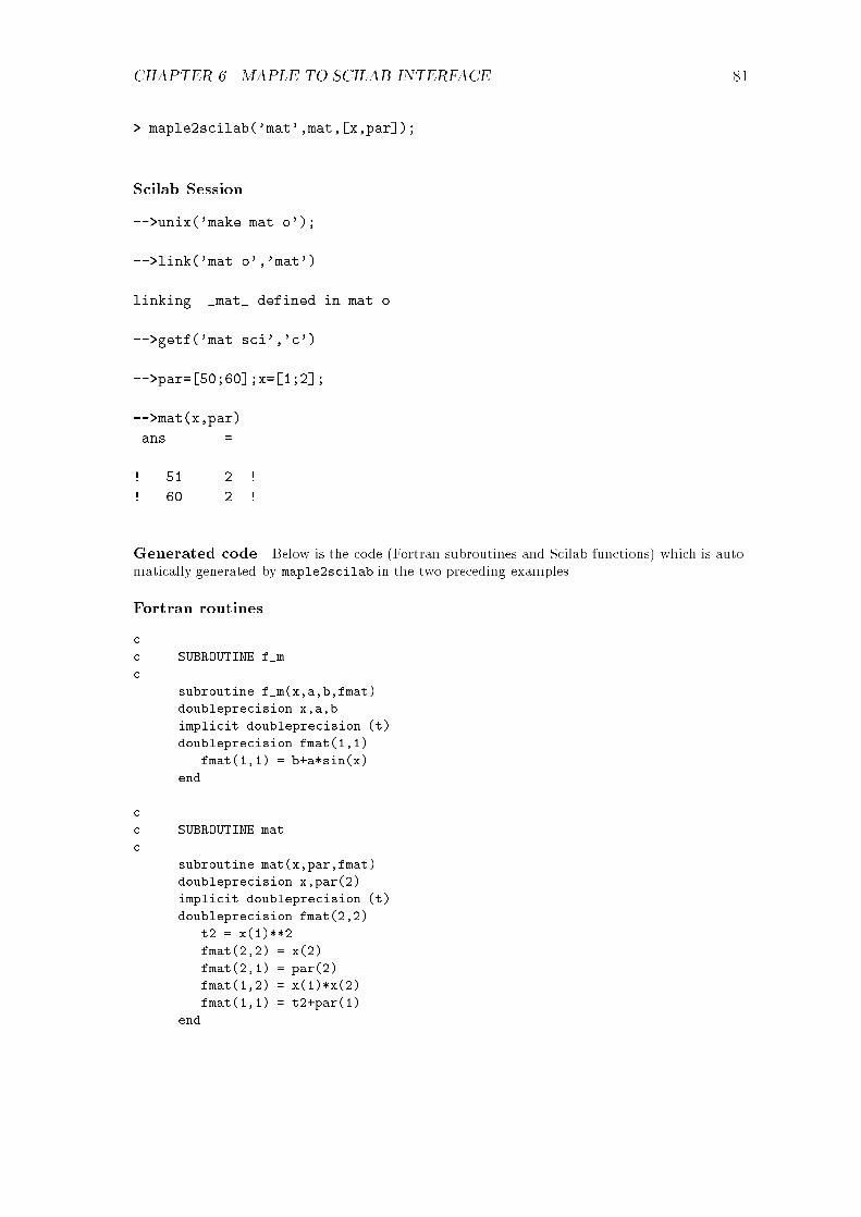
CHAPTER 6. MAPLE TO SCILAB INTERFACE 81
> maple2scilab('mat',mat,[x,par]);
Scilab Session
-->unix('make mat.o');
-->link('mat.o','mat')
linking _mat_ defined in mat.o
-->getf('mat.sci','c')
-->par=[50;60];x=[1;2];
-->mat(x,par)
ans =
! 51. 2. !
! 60. 2. !
Generated code Below is the code (Fortran subroutines and Scilab functions) which is auto-matically generated by maple2scilab in the two preceding examples.
Fortran routines
c
c SUBROUTINE f_m
c
subroutine f_m(x,a,b,fmat)
doubleprecision x,a,b
implicit doubleprecision (t)
doubleprecision fmat(1,1)
fmat(1,1) = b+a*sin(x)
end
c
c SUBROUTINE mat
c
subroutine mat(x,par,fmat)
doubleprecision x,par(2)
implicit doubleprecision (t)
doubleprecision fmat(2,2)
t2 = x(1)**2
fmat(2,2) = x(2)
fmat(2,1) = par(2)
fmat(1,2) = x(1)*x(2)
fmat(1,1) = t2+par(1)
end

CHAPTER 6. MAPLE TO SCILAB INTERFACE 82
Scilab functions
function [var]=f_m(x,a,b)
var=fort('f_m',x,1,'d',a,2,'d',b,3,'d','out',[1,1],4,'d')
//end
function [var]=fmat(x,par)
var=fort('fmat',x,1,'d',par,2,'d','out',[2,2],3,'d')
//end

Appendix A
A demo session
We give here the Scilab session corresponding to the �rst demo.
-->//SCILAB OBJECTS 1. SCALARS
-->a=1 //constant
a =
1.
-->1==1 //boolean
ans =
T
-->'string' //character string
ans =
string
-->z=poly(0,'z') // polynomial with variable 'z' and with one root at zero
z =
z
-->p=1+3*z+4.5*z^2 //polynomial
p =
2
1 + 3z + 4.5z
-->r=z/p //rational
r =
z
-------------
2
83

APPENDIX A. A DEMO SESSION 84
1 + 3z + 4.5z
-->//SCILAB OBJECTS 2. MATRICES
-->a=[a+1 2 3
0 0 atan(1)
5 9 -1] //constant matrix
a =
! 2. 2. 3. !
! 0. 0. 0.7853982 !
! 5. 9. - 1. !
-->b=[%t,%f] //boolean matrix
b =
! T F !
-->mc=['this','is';
'a' ,'matrix'] //matrix of strings
mc =
!this is !
! !
!a matrix !
-->mp=[p,1-z;
1,z*p] //polynomial matrix
mp =
! 2 !
! 1 + 3z + 4.5z 1 - z !
! !
! 2 3 !
! 1 z + 3z + 4.5z !
-->mp=[p 1-z]
mp =
! 2 !
! 1 + 3z + 4.5z 1 - z !
-->mp=[mp;1 1+z*p] //matrix polynomial
mp =
! 2 !
! 1 + 3z + 4.5z 1 - z !
! !

APPENDIX A. A DEMO SESSION 85
! 2 3 !
! 1 1 + z + 3z + 4.5z !
-->f=mp/poly([1+%i 1-%i 1],'z') //rational matrix
f =
! 2 !
! 1 + 3z + 4.5z - 1 !
! --------------- --------- !
! 2 3 2 !
! - 2 + 4z - 3z + z 2 - 2z + z !
! !
! 2 3 !
! 1 1 + z + 3z + 4.5z !
! --------------- ----------------- !
! 2 3 2 3 !
! - 2 + 4z - 3z + z - 2 + 4z - 3z + z !
-->//SCILAB OBJECTS 3. LISTS
-->l=list(a,-(1:5), mp,['this','is';'a','list']) //list
l =
l>1
! 2. 2. 3. !
! 0. 0. 0.7853982 !
! 5. 9. - 1. !
l>2
! - 1. - 2. - 3. - 4. - 5. !
l>3
! 2 !
! 1 + 3z + 4.5z 1 - z !
! !
! 2 3 !
! 1 1 + z + 3z + 4.5z !
l>4
!this is !
! !
!a list !

APPENDIX A. A DEMO SESSION 86
-->b=[1 0;0 1;0 0];c=[1 -1 0];d=0*c*b;x0=[0;0;0];
-->sl=syslin('c',a,b,c,d,x0) //Linear system in state-space representation.
sl =
sl(1) (state-space system:)
lss
sl(2) = A matrix =
! 2. 2. 3. !
! 0. 0. 0.7853982 !
! 5. 9. - 1. !
sl(3) = B matrix =
! 1. 0. !
! 0. 1. !
! 0. 0. !
sl(4) = C matrix =
! 1. - 1. 0. !
sl(5) = D matrix =
! 0. 0. !
sl(6) = X0 (initial state) =
! 0. !
! 0. !
! 0. !
sl(7) = Time domain =
c
-->slt=ss2tf(sl) // Transfer matrix
slt =
! 2 2 !
! - 10.995574 + s + s 46 + 3s - s !
! ----------------------------- ----------------------------- !
! 2 3 2 !
! 6.2831853 - 24.068583s - s + s 6.2831853 - 24.068583s - s !

APPENDIX A. A DEMO SESSION 87
! 3 !
! + s !
-->// OPERATIONS
-->v=1:5;v*v' //constant matrix
ans =
55.
-->mp'*mp+eye //polynomial matrix
ans =
! 2 3 4 2 !
! 3 + 6z + 18z + 27z + 20.25z 2 + 3z + 4.5z !
! !
! 2 2 3 4 5 6 !
! 2 + 3z + 4.5z 3 + 8z + 15z + 18z + 27z + 20.25z !
-->mp1=mp(1,1)+4.5*%i //complex
mp1 =
real part
2
1 + 3z + 4.5z
imaginary part
4.5
-->fi=c*(z*eye-a)^(-1)*b; //transfer function evaluation
-->f(:,1)*fi //rationals
ans =
column 1
! 2 3 4 !
! - 10.995574 - 31.986723z - 45.480084z + 7.5z + 4.5z !
! ----------------------------------------------------------------- !
! 2 3 4 !
! - 12.566371 + 73.269908z - 113.12389z + 72.488936z - 17.068583z !
! 5 6 !
! - 4z + z !
! !

APPENDIX A. A DEMO SESSION 88
! 2 !
! - 10.995574 + z + z !
! ----------------------------------------------------------------- !
! 2 3 4 !
! - 12.566371 + 73.269908z - 113.12389z + 72.488936z - 17.068583z !
! 5 6 !
! - 4z + z !
column 2
! 2 3 4 !
! 46 + 141z + 215z + 10.5z - 4.5z !
! ----------------------------------------------------------------- !
! 2 3 4 !
! - 12.566371 + 73.269908z - 113.12389z + 72.488936z - 17.068583z !
! 5 6 !
! - 4z + z !
! !
! 2 !
! 46 + 3z - z !
! ----------------------------------------------------------------- !
! 2 3 4 !
! - 12.566371 + 73.269908z - 113.12389z + 72.488936z - 17.068583z !
! 5 6 !
! - 4z + z !
-->m=[mp -mp; mp' mp+eye] //usual Matlab syntax for polynomials
m =
column 1 to 3
! 2 2 !
! 1 + 3z + 4.5z 1 - z - 1 - 3z - 4.5z !
! !
! 2 3 !
! 1 1 + z + 3z + 4.5z - 1 !
! !
! 2 2 !
! 1 + 3z + 4.5z 1 2 + 3z + 4.5z !
! !
! 2 3 !
! 1 - z 1 + z + 3z + 4.5z 1 !
column 4
! - 1 + z !
! !

APPENDIX A. A DEMO SESSION 89
! 2 3 !
! - 1 - z - 3z - 4.5z !
! !
! 1 - z !
! !
! 2 3 !
! 2 + z + 3z + 4.5z !
-->[fi, fi(:,1)] // ... or rationals
ans =
column 1 to 2
! 2 2 !
! - 10.995574 + z + z 46 + 3z - z !
! ----------------------------- ----------------------------- !
! 2 3 2 !
! 6.2831853 - 24.068583z - z + z 6.2831853 - 24.068583z - z !
! 3 !
! + z !
column 3
! 2 !
! - 10.995574 + z + z !
! ----------------------------- !
! 2 3 !
! 6.2831853 - 24.068583z - z + z !
-->f=syslin('c',f);
-->num=f(2);den=f(3); //operation on transfer matrix
-->// SOME NUMERICAL PRIMITIVES
-->inv(a) //Inverse
ans =
! 1.125 - 4.6154933 - 0.25 !
! - 0.625 2.705634 0.25 !
! 0. 1.2732395 0. !
-->inv(mp) //Inverse
ans =
! 2 3 !
! - 1 - z - 3z - 4.5z 1 - z !

APPENDIX A. A DEMO SESSION 90
! ------------------------------- ------------------------------- !
! 2 3 4 5 2 3 4 !
! - 5z - 10.5z - 18z - 27z - 20.25z - 5z - 10.5z - 18z - 27z !
! 5 !
! - 20.25z !
! !
! 2 !
! 1 - 1 - 3z - 4.5z !
! ------------------------------- ------------------------------- !
! 2 3 4 5 2 3 4 !
! - 5z - 10.5z - 18z - 27z - 20.25z - 5z - 10.5z - 18z - 27z !
! 5 !
! - 20.25z !
-->inv(sl*sl') //Product of two linear systems and inverse
ans =
ans(1) (state-space system:)
lss
ans(2) = A matrix =
! 5.9830447 - 2.7428339 7.3183626 - 4.2885178 !
! 2.6071355 6.0712325 - 7.7859471 - 5.4755708 !
! 0. - 1.998D-15 - 4.9854125 - 0.7866233 !
! 0. 3.220D-15 0.5793044 - 5.0688648 !
ans(3) = B matrix =
! - 12.503402 !
! - 6.1225032 !
! 2.1610821 !
! - 2.2230824 !
ans(4) = C matrix =
! - 0.9983022 4.0965198 - 7.074889 0.1816573 !
ans(5) = D matrix =
2
2.4292037 - 9.021D-17s + 0.5s
ans(6) = X0 (initial state) =
! 0. !

APPENDIX A. A DEMO SESSION 91
! 0. !
! 0. !
! 0. !
ans(7) = Time domain =
c
-->w=ss2tf(ans) //Transfer function representation
w =
2 3 4
19.739209 - 151.22737s + 283.36517s + 30.351769s - 23.568583s
5 6
- s + 0.5s
------------------------------------------------------------------
2 3 4
1118.4513 + 127.00443s - 51.995574s - 2s + s
-->inv(ss2tf(sl)*ss2tf(sl')) //Product of two transfer functions and inverse
ans =
2 3 4
39.478418 - 302.45474s + 566.73034s + 60.703538s - 47.137167s
5 6
- 2s + s
------------------------------------------------------------------
2 3 4
2236.9027 + 254.00885s - 103.99115s - 4s + 2s
-->clean(w-ans)
ans =
0
-
1
-->n=contr(a,b) //Controllability
n =
3.
-->k=ppol(a,b,[-1-%i -1+%i -1]) //Pole placement
k =
! 0.1832061 - 0.3358779 1.740458 !
! 2.7463953 3.8167939 1.7650419 !

APPENDIX A. A DEMO SESSION 92
-->poly(a-b*k,'z')-poly([-1-%i -1+%i -1],'z') //Check...
ans =
2
- 2.154D-14 + 2.665D-15z
-->s=sin(0:0.1:5*%pi);
-->ss=fft(s(1:128),-1); //FFT
-->xbasc();
-->plot2d3("enn",1,abs(ss)'); //simple plot
-->x=lyap(a,diag([1 2 3]),'cont') //Lyapunov equation
x =
! - 1.4958251 - 4.3299851 0.6983300 !
! - 4.3299851 - 0.3504060 1.07333 !
! 0.6983300 1.07333 1.4379815 !
-->// ON LINE DEFINITION OF MACRO
-->deff('[x]=fact(n)','if n=0 then x=1,else x=n*fact(n-1),end')
-->10+fact(5)
ans =
130.
-->// OPTIMIZATION
-->deff('[f,g,ind]=rosenbro(x,ind)', 'a=x(2)-x(1)^2 , b=1-x(2) ,...
f=100.*a^2 + b^2 , g(1)=-400.*x(1)*a , g(2)=200.*a -2.*b ');
-->comp(rosenbro);[f,x,g]=optim(rosenbro,[2;2],'qn')
norm of projected gradient lower than 0.0000000D+00
g =
! 0. !
! 0. !
x =
! 1. !
! 1. !
f =

APPENDIX A. A DEMO SESSION 93
0.
-->// SIMULATION
-->a=rand(3,3)
a =
! 0.3616361 0.4826472 0.5015342 !
! 0.2922267 0.3321719 0.4368588 !
! 0.5664249 0.5935095 0.2693125 !
-->e=exp(a)
e =
! 1.8016766 0.9861359 0.9295708 !
! 0.6462788 1.7366226 0.7731203 !
! 1.0024892 1.1047133 1.7455217 !
-->deff('[ydot]=f(t,y)','ydot=a*y');comp(f)
-->e(:,1)-ode([1;0;0],0,1,f)
ans =
! - 6.303D-08 !
! - 5.028D-08 !
! - 6.558D-08 !
-->// SYSTEM DEFINITION
-->s=poly(0,'s')
s =
s
-->h=[1/s,1/(s+1);1/s/(s+1),1/(s+2)/(s+2)]
h =
! 1 1 !
! - ----- !
! s 1 + s !
! !
! 1 1 !
! ----- --------- !
! 2 2 !
! s + s 4 + 4s + s !
-->w=tf2ss(h);

APPENDIX A. A DEMO SESSION 94
-->ss2tf(w)
ans =
! 1 1 !
! ------------- ----- !
! 2.512D-15 + s 1 + s !
! !
! 1 + 5.884D-15s 1 + 5.148D-15s !
! ---------------- -------------- !
! 2 2 !
! 4.050D-14 + s + s 4 + 4s + s !
-->h1=clean(ans)
h1 =
! 1 1 !
! - ----- !
! s 1 + s !
! !
! 1 1 !
! ----- --------- !
! 2 2 !
! s + s 4 + 4s + s !
-->// EXAMPLE: SECOND ORDER SYSTEM ANALYSIS
-->sl=syslin('c',1/(s*s+0.2*s+1))
sl =
1
-----------
2
1 + 0.2s + s
-->instants=0:0.05:20;
-->// step response:
-->y=csim('step',instants,sl);
-->xbasc();plot2d(instants',y')
-->// Delayed step response
-->deff('[in]=u(t)','if t<3 then in=0;else in=1;end');
-->comp(u);

APPENDIX A. A DEMO SESSION 95
-->y1=csim(u,instants,sl);plot2d(instants',y1');
-->// Impulse response;
-->yi=csim('imp',instants,sl);xbasc();plot2d(instants',yi');
-->yi1=csim('step',instants,s*sl);plot2d(instants',yi1');
-->// Discretization
-->dt=0.05;
-->sld=dscr(tf2ss(sl),0.05);
-->// Step response
-->u=ones(instants);
Warning :redefining function: u
-->yyy=flts(u,sld);
-->xbasc();plot(instants,yyy)
-->// Impulse response
-->u=0*ones(instants);u(1)=1/dt;
-->yy=flts(u,sld);
-->xbasc();plot(instants,yy)
-->// system interconnexion
-->w1=[w,w];
-->clean(ss2tf(w1))
ans =
! 1 1 1 1 !
! - ----- - ----- !
! s 1 + s s 1 + s !
! !
! 1 1 1 1 !
! ----- --------- ----- --------- !
! 2 2 2 2 !
! s + s 4 + 4s + s s + s 4 + 4s + s !
APPENDIX A. A DEMO SESSION 96
-->w2=[w;w];
-->clean(ss2tf(w2))
ans =
! 1 1 !
! - ----- !
! s 1 + s !
! !
! 1 1 !
! ----- --------- !
! 2 2 !
! s + s 4 + 4s + s !
! !
! 1 1 !
! - ----- !
! s 1 + s !
! !
! 1 1 !
! ----- --------- !
! 2 2 !
! s + s 4 + 4s + s !
-->// change of variable
-->z=poly(0,'z');
-->horner(h,(1-z)/(1+z)) //bilinear transform
ans =
! 1 + z 1 + z !
! ----- ----- !
! 1 - z 2 !
! !
! 2 2 !
! 1 + 2z + z 1 + 2z + z !
! ---------- ---------- !
! 2 !
! 2 - 2z 9 + 6z + z !
-->// PRIMITIVES
-->H=[1. 1. 1. 0.;
2. - 1. 0. 1;
1. 0. 1. 1.;
0. 1. 2. - 1];
-->ww=spec(H)

APPENDIX A. A DEMO SESSION 97
ww =
! 2.7320508 !
! - 2.7320508 !
! 0.7320508 !
! - 0.7320508 !
-->// STABLE SUBSPACES
-->[X,d]=schur(H,'cont');
-->X'*H*X
ans =
! - 2.7320508 - 1.110D-15 0. 1. !
! 0. - 0.7320508 - 1. - 7.772D-16 !
! 7.216D-16 0. 2.7320508 0. !
! 0. - 6.106D-16 0. 0.7320508 !
-->[X,d]=schur(H,'disc');
-->X'*H*X
ans =
! 0.7320508 0. 7.772D-16 1. !
! 0. - 0.7320508 - 1. 8.604D-16 !
! 0. 0. 2.7320508 - 1.166D-15 !
! 7.772D-16 1.110D-15 - 1.277D-15 - 2.7320508 !
-->//Selection of user-defined eigenvalues (# 3 and 4 here);
-->deff('[flg]=sel(x)','flg=0,ev=x(2)/x(3),if abs(ev-ww(3))<0.0001|abs(ev-ww(4))<0.00001
-->[X,d]=schur(H,sel)
d =
2.
X =
! - 0.5705632 - 0.2430494 - 0.6640233 - 0.4176813 !
! - 0.4176813 0.6640233 - 0.2430494 0.5705632 !
! 0.5705632 - 0.2430494 - 0.6640233 0.4176813 !
! 0.4176813 0.6640233 - 0.2430494 - 0.5705632 !
-->X'*H*X
ans =
! 0.7320508 0. 7.772D-16 1. !

APPENDIX A. A DEMO SESSION 98
! 0. - 0.7320508 - 1. 8.604D-16 !
! 0. 0. 2.7320508 - 1.166D-15 !
! 7.772D-16 1.110D-15 - 1.277D-15 - 2.7320508 !
-->// With matrix pencil
-->[X,d]=gschur(H,eye(H),sel)
d =
2.
X =
! 0.5705632 0.2430494 0.6640233 0.4176813 !
! 0.4176813 - 0.6640233 0.2430494 - 0.5705632 !
! - 0.5705632 0.2430494 0.6640233 - 0.4176813 !
! - 0.4176813 - 0.6640233 0.2430494 0.5705632 !
-->X'*H*X
ans =
! 0.7320508 0. 9.576D-16 1. !
! 0. - 0.7320508 - 1. 0. !
! 8.882D-16 0. 2.7320508 0. !
! 0. 0. 0. - 2.7320508 !
-->// block diagonalization
-->[ab,x,bs]=bdiag(H);
-->inv(x)*H*x
ans =
! 2.7320508 1.610D-15 0. 0. !
! - 3.664D-15 - 2.7320508 0. 6.661D-16 !
! 0. 0. 0.7320508 - 7.910D-16 !
! 0. 0. 0. - 0.7320508 !
-->// Matrix pencils
-->E=rand(3,2)*rand(2,3);
-->A=rand(3,2)*rand(2,3);
-->s=poly(0,'s');
-->w=det(s*D-A) //determinant
w =

APPENDIX A. A DEMO SESSION 99
2
- 0.0801176s + 0.0423727s
-->[al,be]=gspec(A,E);
-->al./(be+%eps*ones(be))
ans =
! 1.687D+15 !
! 1.8907826 !
! - 7.445D-17 !
-->roots(w)
ans =
! 0 !
! 1.8907826 !
-->[Ns,d]=coffg(s*D-A); //inverse of polynomial matrix;
-->clean(Ns/d*(s*D-A))
ans =
! 1 0 0 !
! - - - !
! 1 1 1 !
! !
! 0 1 0 !
! - - - !
! 1 1 1 !
! !
! 0 0 1 !
! - - - !
! 1 1 1 !
-->[Q,M,i1]=pencan(E,A); // Canonical form;
rank A^k rcond
2. 0.347D+00
rank A^k rcond
2. 0.552D+00
-->M*E*Q
ans =
! 1. 3.608D-16 0. !
! 9.576D-16 1. - 3.331D-16 !
! 8.077D-16 - 3.655D-16 0. !

APPENDIX A. A DEMO SESSION 100
-->M*A*Q
ans =
! 1.8609512 - 0.4018602 0. !
! - 0.1381447 0.0298314 0. !
! 0. 6.661D-16 1. !
-->// PAUSD-RESUME
-->write(%io(2),'pause command...');
pause command...
-->write(%io(2),'TO CONTINUE...');
TO CONTINUE...
-->write(%io(2),'ENTER ''resume (or return) or click on resume!!''');
ENTER 'resume (or return) or click on resume!!'
-->pause;
-1->resume;
-->// CALLING EXTERNAL ROUTINE
-->foo=[' subroutine foo(a,b,c)';
' c=a+b';
' end' ];
-->unix_s('\rm foo.f')
-->write('foo.f',foo);
-->unix_s('make foo.o') //Compiling...(needs fortran compiler)
-->//..................WARNING.......................
-->//NEXT COMMAND LINE WILL DO THE LINK OF THE ROUTINE foo WITH SCILAB
-->//THIS COMMAND MAY FAIL FOR SystemV COMPILED VERSIONS OF SCILAB
-->//BECAUSE LINK NEEDS THE LIBRARIES (SEE THE HELP OF "LINK" COMMAND)
-->link('foo.o','foo') //Linking to Scilab
-->//5+7 by fortran
-->fort('foo',5,1,'r',7,2,'r','out',[1,1],3,'r')
ans =

APPENDIX A. A DEMO SESSION 101
12.
-->

List of Figures
1.1 A Simple Response : : : : : : : : : : : : : : : : : : : : : : : : : : : : : : : : 171.2 Phase Plot : : : : : : : : : : : : : : : : : : : : : : : : : : : : : : : : : : : : 18
2.1 Inter-Connection of Linear Systems : : : : : : : : : : : : : : : : : : : : : : : 33
4.1 Simulation of a Double Pendulum : : : : : : : : : : : : : : : : : : : : : : : : 514.2 Optimal Lifeguard Path : : : : : : : : : : : : : : : : : : : : : : : : : : : : : 544.3 Inter-Connected Systems : : : : : : : : : : : : : : : : : : : : : : : : : : : : : 56
5.1 First example of plotting : : : : : : : : : : : : : : : : : : : : : : : : : : : : : 645.2 Simple 2D Plot : : : : : : : : : : : : : : : : : : : : : : : : : : : : : : : : : : 675.3 Some Capabilities of 2D Plot : : : : : : : : : : : : : : : : : : : : : : : : : : 685.4 Use of plotframe : : : : : : : : : : : : : : : : : : : : : : : : : : : : : : : : : 685.5 Geometric Graphics and Comments : : : : : : : : : : : : : : : : : : : : : : 705.6 2D and 3D plot : : : : : : : : : : : : : : : : : : : : : : : : : : : : : : : : : : 715.7 Use of xsetech : : : : : : : : : : : : : : : : : : : : : : : : : : : : : : : : : : : 725.8 Group of �gures : : : : : : : : : : : : : : : : : : : : : : : : : : : : : : : : : 735.9 Blatexp2 Example : : : : : : : : : : : : : : : : : : : : : : : : : : : : : : : : 765.10 Encapsulated Postscript by Using X�g : : : : : : : : : : : : : : : : : : : : : 78
102

Index
A
ans : : : : : : : : : : : : : : : : : : : : : : : : : : : : : : : : : : 8argn : : : : : : : : : : : : : : : : : : : : : : : : : : : : : : : : 43
B
bloc2exp : : : : : : : : : : : : : : : : : : : : : : : : : : : 56boolean : : : : : : : : : : : : : : : : : : : : : : : : : : : : : 28break : : : : : : : : : : : : : : : : : : : : : : : : : : : : : : :43
C
C : : : : : : : : : : : : : : : : : : : : : : : : : : : : : : : : : : : 53character strings : : : : : : : : : : : : : : : : : : : : 24clear : : : : : : : : : : : : : : : : : : : : : : : : : : : : : : :48constants : : : : : : : : : : : : : : : : : : : : : : : : : : : :19
D
data types : : : : : : : : : : : : : : : : : : : : : : : : : : 19booleans : : : : : : : : : : : : : : : : : : : : : : : : 28character strings : : : : : : : : : : : : : : : : 24constants : : : : : : : : : : : : : : : : : : : : : : : 19functions : : : : : : : : : : : : : : : : : : : : : : : :35libraries : : : : : : : : : : : : : : : : : : : : : : : : :36lists : : : : : : : : : : : : : : : : : : : : : : : : : : : : :29matrices : : : : : : : : : : : : : : : : : : : : :19, 23polynomials : : : : : : : : : : : : : : : : : : : : : 27
deff : : : : : : : : : : : : : : : : : : : : : : : : : : : : : : : : 35
E
environment : : : : : : : : : : : : : : : : : : : : : : : : :48error : : : : : : : : : : : : : : : : : : : : : : : : : : : : : : :43evstr : : : : : : : : : : : : : : : : : : : : : : : : : : : : : : :56exists : : : : : : : : : : : : : : : : : : : : : : : : : : : : : :41external : : : : : : : : : : : : : : : : : : : : : : : : : : : : :49
F
for : : : : : : : : : : : : : : : : : : : : : : : : : : : : : : : : : 38fort : : : : : : : : : : : : : : : : : : : : : : : : : : : : : : : : 53Fortran : : : : : : : : : : : : : : : : : : : : : : : : : : : : : 53functions : : : : : : : : : : : : : : : : : : : : : : : : : : : :35
deff : : : : : : : : : : : : : : : : : : : : : : : : : : : : 35
G
getf : : : : : : : : : : : : : : : : : : : : : : : : : : : : 40, 48
H
help : : : : : : : : : : : : : : : : : : : : : : : : : : : : : : : : 48
I
if-then-else : : : : : : : : : : : : : : : : : : : : : : :39input : : : : : : : : : : : : : : : : : : : : : : : : : : : : : : : :49interf : : : : : : : : : : : : : : : : : : : : : : : : : : : : : :53interfacing fortran : : : : : : : : : : : : : : : : : : :53
L
lib : : : : : : : : : : : : : : : : : : : : : : : : : : : : : : : : : 48libraries : : : : : : : : : : : : : : : : : : : : : : : : : 36, 48linear systems
ss2tf : : : : : : : : : : : : : : : : : : : : : : : : : : :33syslin : : : : : : : : : : : : : : : : : : : : : : : : : :35tf2ss : : : : : : : : : : : : : : : : : : : : : : : : : : :33inter-connection of : : : : : : : : : : :33, 56
link : : : : : : : : : : : : : : : : : : : : : : : : : : : : : : : : 53lists : : : : : : : : : : : : : : : : : : : : : : : : : : : : : : : : : 29load : : : : : : : : : : : : : : : : : : : : : : : : : : : : : : : : 48
M
macros : : : : : : : : : : : : : : : : : : : : : : : : : : : : : : 40exists : : : : : : : : : : : : : : : : : : : : : : : : : :41getf : : : : : : : : : : : : : : : : : : : : : : : : : : : : 40de�nition : : : : : : : : : : : : : : : : : : : : : : : 40
Maple : : : : : : : : : : : : : : : : : : : : : : : : : : : : : : :79maple2scilab : : : : : : : : : : : : : : : : : : : : : : :79matrices : : : : : : : : : : : : : : : : : : : : : : : : : : : : 23
block construction : : : : : : : : : : : : : : :23constant : : : : : : : : : : : : : : : : : : : : : : : : 23
matrix : : : : : : : : : : : : : : : : : : : : : : : : : : : : : :24
N
non-linear calculation : : : : : : : : : : : : : : : 49
O
ones : : : : : : : : : : : : : : : : : : : : : : : : : : : : 22, 23operations
for new data types : : : : : : : : : : : : : : 44
103

INDEX 104
optim : : : : : : : : : : : : : : : : : : : : : : : : : : : : : : :52optimization : : : : : : : : : : : : : : : : : : : : : : : : 49output : : : : : : : : : : : : : : : : : : : : : : : : : : : : : : 49
P
pause : : : : : : : : : : : : : : : : : : : : : : : : : : : 10, 43poly : : : : : : : : : : : : : : : : : : : : : : : : : : : : : : : : 27polynomials : : : : : : : : : : : : : : : : : : : : : : : : : 27programming : : : : : : : : : : : : : : : : : : : : : : : :37
comparison operators : : : : : : : : : : : :37conditionals : : : : : : : : : : : : : : : : : : : : : 39loops : : : : : : : : : : : : : : : : : : : : : : : : : : : :38macros : : : : : : : : : : : : : : : : : : : : : : : : : :40
R
read : : : : : : : : : : : : : : : : : : : : : : : : : : : : : : : : 49regulator : : : : : : : : : : : : : : : : : : : : : : : : : : : :56return : : : : : : : : : : : : : : : : : : : : : : : : : : 10, 43
S
save : : : : : : : : : : : : : : : : : : : : : : : : : : : : : : : : 48scalars : : : : : : : : : : : : : : : : : : : : : : : : : : : : : : 19select-case : : : : : : : : : : : : : : : : : : : : : : : : 39signals
saving and loading : : : : : : : : : : : : : : : 1simulation : : : : : : : : : : : : : : : : : : : : : : : : : : :49ss2tf : : : : : : : : : : : : : : : : : : : : : : : : : : : : : : :33startup by user : : : : : : : : : : : : : : : : : : : : : :48startup.sci : : : : : : : : : : : : : : : : : : : : : : : :48symbolic triangularization : : : : : : : : : : : 25syslin : : : : : : : : : : : : : : : : : : : : : : : : : : : : : :35
T
tf2ss : : : : : : : : : : : : : : : : : : : : : : : : : : : : : : :33trianfml : : : : : : : : : : : : : : : : : : : : : : : : : : : 25
V
vectors : : : : : : : : : : : : : : : : : : : : : : : : : : : : : :20constant : : : : : : : : : : : : : : : : : : : : : : : : 22incremental : : : : : : : : : : : : : : : : : : : : : 21transpose : : : : : : : : : : : : : : : : : : : : : : : 21
W
warning : : : : : : : : : : : : : : : : : : : : : : : : : : : : 43while : : : : : : : : : : : : : : : : : : : : : : : : : : : : : : :38who : : : : : : : : : : : : : : : : : : : : : : : : : : : : : : : : : 48write : : : : : : : : : : : : : : : : : : : : : : : : : : : : : : :49


![Messgeräte - Klaus Betzler's Homepage · 2 Elektronik–Praktikum Physik 1 Oszilloskop Das am Arbeitsplatz verwendete Oszilloskop TDS210 der Firma Tek-tronix[1] ist ein Digitalspeichergerät](https://img.dokumen.tips/doc/110x75/5c9e8e9588c993362d8bc862/messgeraete-klaus-betzlers-homepage-2-elektronikpraktikum-physik-1-oszilloskop.jpg)