Embed Size (px)
Citation preview

* Department of Economics and Department of Mathematics, Stanford University, [email protected] + Department of Computer Science and Department of Statistics, Stanford University, [email protected] ‡ Department of Economics, Department of Management Science and Engineering, Department of Mathematical and Computational Science, Stanford University, [email protected] † Department of Computer Science, Stanford University, [email protected]
Reconstructing the Order Book
Kunal Khanna*, Michael Smith+, David Wu‡ and Tony Zhang†
June 2009
Abstract
Statistical properties concerning the shape of the order book have been studied in some detail but literature on the evolution of the order book over time has been lacking. This paper presents a thorough analysis of the empirical properties of the order book, focusing on the time dimension. Following an empirical analysis we present a self-exciting point process model for the arrival of orders. We end with an application of our model to high frequency trading.
Acknowledgements
We would like to thank Kay Giesecke and Gerry Tsoukalas for their advice and guidance. We would also like to thank Jeremy Evnine and Lisa Borland for defining a problem for us to work on and providing the data for it.

2
1. Introduction
While studies of financial markets often focus on the prices of traded assets, little attention is paid to the manner in which these prices are determined. Prices for traded securities depend on the interplay between buy and sell orders submitted by market participants. Until fairly recently, the execution of these buy and sell orders was determined by centralized market makers who provided quotes at which they were willing to buy and sell, in what is known as a quote-driven market.
With the advent of electronic trading, markets have moved to a system in which liquidity provision has become decentralized. Now most markets are order-driven, where any market participant is free to provide liquidity by submitting a buy or sell order. Submitted orders are amalgamated by price to create a limit order book. The rule driven execution of orders in these limit order books and the extensive data that is available for order driven markets makes them ideal candidates for stochastic modeling.
We approach the problem of modeling the order book by first considering its empirical properties. Biais et al. (1995), Bouchaud et al. (2002), Smith et al. (2003) and Foucault et al. (2005) have conducted work on the shape of the order book. They have found that the order book of a variety of stocks, across markets, display universal properties that correspond to a type of power law. We attempt to reproduce their results on the current data of two highly liquid stocks on the NASDAQ. This is a worthwhile exercise because, while their results have been universal, they have not been tested on a market as liquid as the NASDAQ nor have they been verified on current market data. The electronic trading world has changed dramatically in the past few years with enormous growth in liquidity provision by electronic market makers and high frequency traders. We believe that these advances may have had an effect on the shape of the order book of stocks.
Aside from the shape of the order book, we look into the evolution of the order book over time. Using the same two stocks, we attempt to uncover the properties of order arrivals, looking at order arrival rates at different times during the day and across different points in the order book. We believe that this is a significant advance on the current literature concerning the empirical properties of the order book. Few, if any, authors have examined the arrival of orders or highlighted the time varying properties that the order book exhibits.
After considering the empirical properties of the order book, we attempt to specify a model that captures these properties. We find that order arrivals display clustering, making a self-exciting point process model the best choice for the arrival of orders. Hewlett (2006) has applied a Hawkes process to the arrival of buy and sell orders in markets but few others have applied such processes to the arrival of limit orders. We follow Hewlett in using a Hawkes process and compare this model to a Poisson process that is more common in the literature (see Cont et al. 2008).
3
An understanding of the shape and evolution of the order book allows for a better understanding of price dynamics in financial markets. Ultimately, it is the interaction between buyers and sellers at the level of the order book that determines the short term movement of prices. This has application to the efficient execution of orders, as in Alfonsi et al. (2007) and Obizhaeva and Wang (2006) and to high frequency trading which relies on the ability to predict price movements over a matter of seconds. We end with a discussion of our model in the context of high frequency trading and present some preliminary results from high frequency trading simulations.
2. Data and the Order Book
Our data set consisted of order arrivals for a ten day period extending from March 9, 2009 to March 20, 2009 (March 14 and 15 were non trading days) on Powershares NASDAQ Exchange Traded Fund (QQQQ) and Apple (AAPL). Each arrival had a buy price and volume and a sell price and volume. The buy quotes represent the amount and price at which the market participant is willing to buy while the sell quotes represent the amount and price at which the market participant is willing to sell. All the buy orders are collected to form the buy side of the limit order book while all the sell orders are collected to form the sell side. The best buy price is referred to as the bid while the best sell price is referred to as the ask. The difference between bid and ask is referred to as the spread. The spread is often an indicator of the level of liquidity in a traded asset with a narrower spread indicating greater liquidity.
In reconstructing the order book, we had to keep track of incoming limit buy and sell orders. If an incoming limit buy order is greater than or equal to the ask then it is classified as a market buy order and if an incoming limit sell order is less than or equal to the bid then it is classified as a market sell order. Market orders are placed by those demanding liquidity since they allow for immediate transactions. The flow of limit and market orders constantly updates the order book.
A further complication in reconstructing the order book is the presence of cancellations and modifications. In the data set we used, cancellations and modifications were noted with a time stamp and identified by a market maker code. Our process for dealing with cancellations and modifications was as follows: when a cancellation arrived, we checked the market maker code to identify the past order that was either being cancelled or modified. If that order had not already been executed then we cancelled the order. In the case of a modification, if the order had not already been executed we modified that order and, if subsequent modification caused this order to be executed, we gave it precedence in execution (for further details on cancellations and modifications see Harris 2003).
Summary statistics for the data are shown in Table 1. As is clear from the table, QQQQ is a significantly more active name than AAPL. The high level of activity in QQQQ and extensive liquidity provision make it an interesting stock to study, especially when compared to previous works that have tended to focus on less liquid stocks. Our data shows a higher proportion of

4
TABLE 1: SUMMARY STATISTICS
QQQQ AAPL
Number of Limit Orders 2,977,648 822,932 Number of Market Orders 2,230,105 619,188 Number of Cancellations 858,109 318,998 Average Size of Limit Orders 305.32 4.41 Average Size of Market Orders 235.31 3.52 Average Size of Cancellations 473.03 3.36 Average Time between Limit Orders 0.008s 0.03s Average Time between Markets Orders 0.01s 0.04s Average Time between Cancellations 0.03s 0.07s
market orders and cancellations than previous works. Bouchaud et al., for example, found that market orders and cancellations comprised 10 percent, each, of all orders, whereas we found both cancellations and market orders to be more common. Similarly, our average order size is relatively smaller than other findings. We attribute these facts to the increased participation of electronic market makers and high frequency firms in the financial markets. These firms look to profit from providing liquidity to financial markets in a quick and efficient manner. They typically do so by sending small orders close to the bid and ask and turning over these transactions quickly to capture a spread. Their speed allows them to send and cancel orders quickly, leading to an increase in the number of cancellations. It also allows liquidity takers such as mutual funds to submit market orders without paying large spreads, thereby leading to an increase in the number of market orders.
3. Shape of the Order Book
In order to study the shape of the order book we need to capture the depth of orders in the limit order book. Let us call 𝑎𝑎(𝑡𝑡) the ask price and 𝑏𝑏(𝑡𝑡)the bid price at any time 𝑡𝑡. We define the
mid quote 𝑚𝑚(𝑡𝑡) = �𝑎𝑎(𝑡𝑡)+𝑏𝑏(𝑡𝑡)2
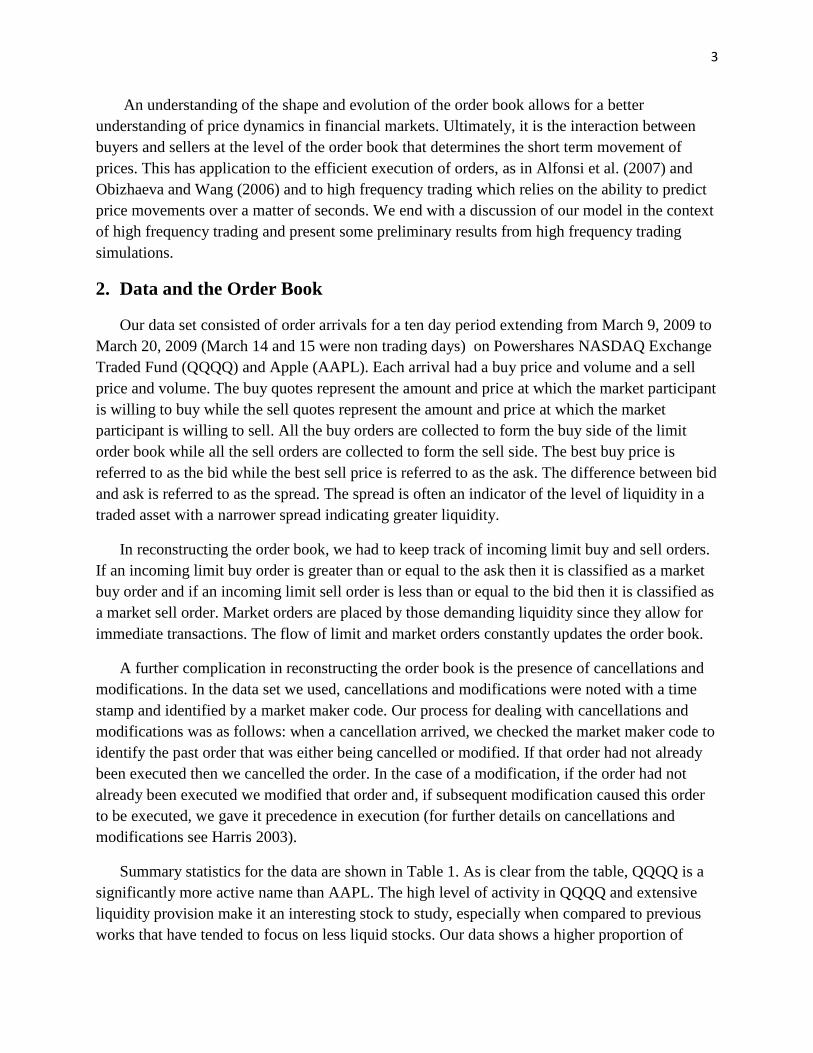
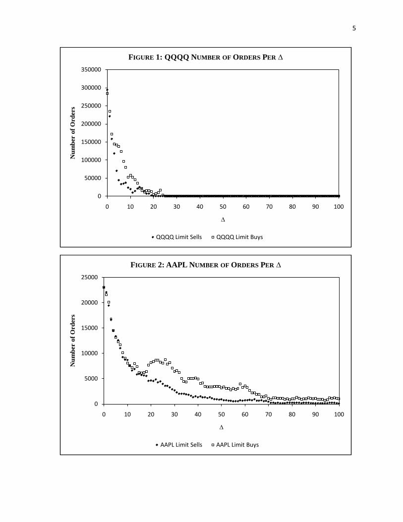
�. The mid quote can be thought of as a price, of sorts, since it gives an indication of where the order book is centered. We also define the spread 𝑠𝑠(𝑡𝑡) = 𝑎𝑎(𝑡𝑡) − 𝑏𝑏(𝑡𝑡). Since both the stocks we are considering are highly liquid, the spread is almost always $0.01 or one tick, the smallest unit of account on the exchange. Lastly, we define ∆ as the distance, in ticks, of an incoming order from the bid or ask. Therefore, 𝑏𝑏(𝑡𝑡) − ∆, for each ∆, captures the depth of the limit buys while 𝑎𝑎(𝑡𝑡) + ∆, captures the depth of limit sells. Note that ∆ can be negative. This would indicate a narrowing of the spread, though such an occurrence is extremely rare in our dataset.
An interesting aspect of the shape of the order book is the density of orders with respect to ∆. Figures 1 and 2 show the number of orders per delta for both limit buys and limit sells. The data confirms some known truths. The majority of orders come in at the bid and ask and orders
5
0
50000
100000
150000
200000
250000
300000
350000
0 10 20 30 40 50 60 70 80 90 100
Num
ber
of O
rder
s
∆
FIGURE 1: QQQQ NUMBER OF ORDERS PER ∆
QQQQ Limit Sells QQQQ Limit Buys
0
5000
10000
15000
20000
25000
0 10 20 30 40 50 60 70 80 90 100
Num
ber
of O
rder
s
∆
FIGURE 2: AAPL NUMBER OF ORDERS PER ∆
AAPL Limit Sells AAPL Limit Buys
6
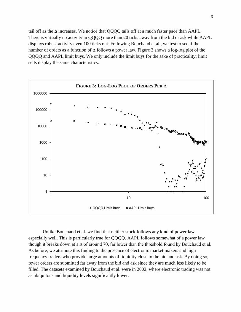
tail off as the ∆ increases. We notice that QQQQ tails off at a much faster pace than AAPL. There is virtually no activity in QQQQ more than 20 ticks away from the bid or ask while AAPL displays robust activity even 100 ticks out. Following Bouchaud et al., we test to see if the number of orders as a function of ∆ follows a power law. Figure 3 shows a log-log plot of the QQQQ and AAPL limit buys. We only include the limit buys for the sake of practicality; limit sells display the same characteristics.
Unlike Bouchaud et al. we find that neither stock follows any kind of power law especially well. This is particularly true for QQQQ. AAPL follows somewhat of a power law though it breaks down at a ∆ of around 70, far lower than the threshold found by Bouchaud et al. As before, we attribute this finding to the presence of electronic market makers and high frequency traders who provide large amounts of liquidity close to the bid and ask. By doing so, fewer orders are submitted far away from the bid and ask since they are much less likely to be filled. The datasets examined by Bouchaud et al. were in 2002, where electronic trading was not as ubiquitous and liquidity levels significantly lower.
1
10
100
1000
10000
100000
1000000
1 10 100
FIGURE 3: LOG-LOG PLOT OF ORDERS PER ∆
QQQQ Limit Buys AAPL Limit Buys
7
0
5000
10000
15000
20000
25000
30000
35000
40000
45000
50000
0 10 20 30 40 50 60 70 80 90 100
Num
ber
of C
ance
ls
∆
FIGURE 4: QQQQ ORDER CANCELLATIONS PER ∆
QQQQ Sell Cancels QQQQ Buy Cancels
0
500
1000
1500
2000
2500
3000
3500
4000
4500
0 10 20 30 40 50 60 70 80 90 100
Axi
s Titl
e
∆
FIGURE 5: AAPL ORDER CANCELLATIONS PER ∆
AAPL Sell Cancels AAPL Buy Cancels

8
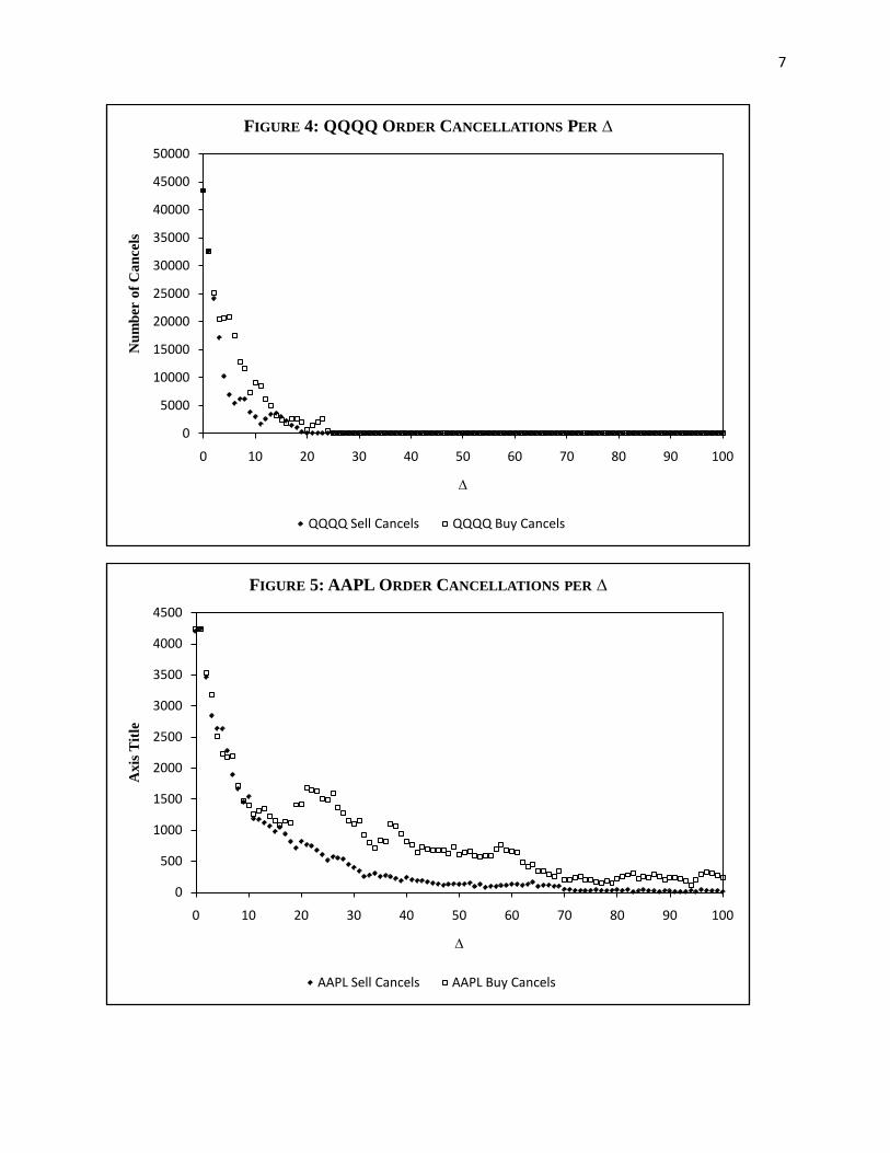
The same analysis can be conducted for cancellations. Figures 4 and 5 show the number of cancellations as a function of ∆ for both stocks. Here, we refer to the ∆ of the quote at the time it is cancelled. As the plots shows, the shape of cancellations mimics that of limit order arrivals. We expect this to be the case if cancellations are a proportion of the orders in queue at a given time, which is a common assumption in the literature (see Cont et al. for example).
The empirical properties of the shape of the order book seem to suggest that the most important aspect of the order book is the bid and ask. Modeling the order book effectively comes down to modeling the bid and ask and, if necessary, the orders that are a few ticks away. This, in turn, relies on some understanding of the evolution of the order book and, in particular, the arrival of orders at the bid and ask.
4. Evolution of the Order Book
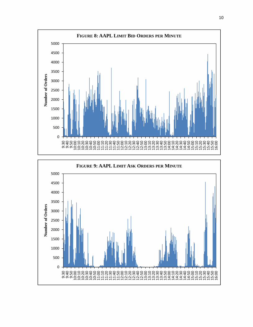
We analyze the arrival of orders at the bid and ask by counting the number of orders per minute through the day. We found that this effectively captures the evolution of the order book and it is not necessary to view arrivals on a smaller time scale. We look at limit bid and ask orders, bid and ask cancellations and market buy and sell orders. Each of these order types allows us to build a complete picture of the order book and understand the dynamics between order arrivals and prices.
Figures 6 through 9 show the arrival of limit bid and ask orders for QQQQ and AAPL on March 9, 2009. The arrival of orders is chaotic with pronounced clustering. Surprisingly, the orders do not exhibit a parabolic shape, with high activity at the beginning and end of the trading day and a lull in the middle. We can use the limit bid and ask arrivals to make predictions about the price of the stock. For example, the period of low activity among limit asks in QQQQ from 12:40 to 13:30 suggests that buy liquidity was being removed from the market. In such a situation we would expect a fall in the price of the stock. Price data from that day indicates that the stock fell almost 4 percent during that period.
The predicative power of order arrivals makes them extremely important when trying to reconstruct the order book. The key feature of arrivals is that they exhibit periods of extremely high and low activity. This property cannot be captured by simple or even parametric Poisson models. Instead, self exciting intensity models, which have the ability to produce clusters, are much more capable of reproducing arrivals that resemble those observed empirically.
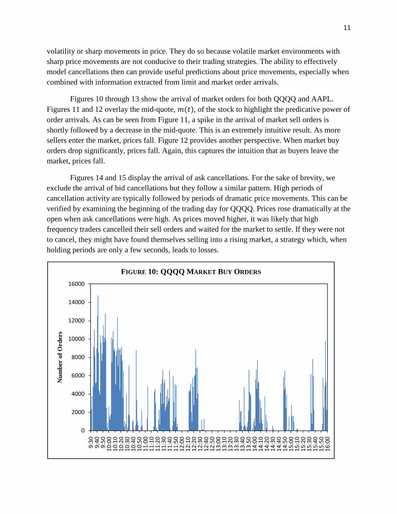
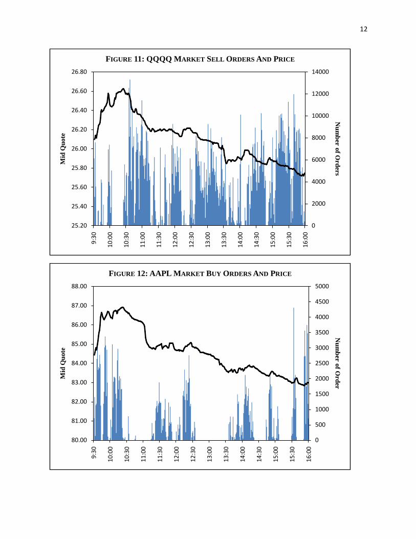
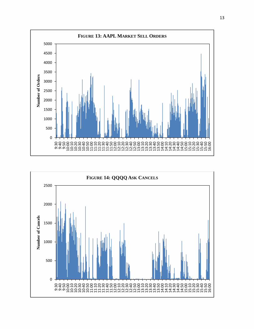
The arrivals of market orders and cancellations for each stock are shown in Figures 10 through 15. Once again, these order types exhibit clustering and seem to adhere more closely to a self-exciting process rather than the more commonly used Poisson process. As with limit orders, the arrivals of markets and, perhaps surprisingly, cancellations convey accurate predictions about price movements over short periods of time. In conversations we had with electronic traders, we were told that often high frequency traders will cancel large numbers of orders during periods of high

9
0
2000
4000
6000
8000
10000
12000
14000
9:30
9:40
9:50
10:0
010
:10
10:2
010
:30
10:4
010
:50
11:0
011
:10
11:2
011
:30
11:4
011
:50
12:0
012
:10
12:2
012
:30
12:4
012
:50
13:0
013
:10
13:2
013
:30
13:4
013
:50
14:0
014
:10
14:2
014
:30
14:4
014
:50
15:0
015
:10
15:2
015
:30
15:4
015
:50
16:0
0
Num
be o
f Ord
ers
FIGURE 6: QQQQ LIMIT BID ORDERS PER MINUTE
0
2000
4000
6000
8000
10000
12000
14000
16000
9:30
9:40
9:50
10:0
010
:10
10:2
010
:30
10:4
010
:50
11:0
011
:10
11:2
011
:30
11:4
011
:50
12:0
012
:10
12:2
012
:30
12:4
012
:50
13:0
013
:10
13:2
013
:30
13:4
013
:50
14:0
014
:10
14:2
014
:30
14:4
014
:50
15:0
015
:10
15:2
015
:30
15:4
015
:50
16:0
0
Num
ber
of O
rder
s
FIGURE 7: QQQQ LIMIT ASK ORDERS PER MINUTE
10
0
500
1000
1500
2000
2500
3000
3500
4000
4500
5000
9:30
9:40
9:50
10:0
010
:10
10:2
010
:30
10:4
010
:50
11:0
011
:10
11:2
011
:30
11:4
011
:50
12:0
012
:10
12:2
012
:30
12:4
012
:50
13:0
013
:10
13:2
013
:30
13:4
013
:50
14:0
014
:10
14:2
014
:30
14:4
014
:50
15:0
015
:10
15:2
015
:30
15:4
015
:50
16:0
0
Num
ber
of O
rder
s
FIGURE 8: AAPL LIMIT BID ORDERS PER MINUTE
0
500
1000
1500
2000
2500
3000
3500
4000
4500
5000
9:30
9:40
9:50
10:0
010
:10
10:2
010
:30
10:4
010
:50
11:0
011
:10
11:2
011
:30
11:4
011
:50
12:0
012
:10
12:2
012
:30
12:4
012
:50
13:0
013
:10
13:2
013
:30
13:4
013
:50
14:0
014
:10
14:2
014
:30
14:4
014
:50
15:0
015
:10
15:2
015
:30
15:4
015
:50
16:0
0
Num
ber
of O
rder
s
FIGURE 9: AAPL LIMIT ASK ORDERS PER MINUTE
11
volatility or sharp movements in price. They do so because volatile market environments with sharp price movements are not conducive to their trading strategies. The ability to effectively model cancellations then can provide useful predictions about price movements, especially when combined with information extracted from limit and market order arrivals.
Figures 10 through 13 show the arrival of market orders for both QQQQ and AAPL. Figures 11 and 12 overlay the mid-quote, 𝑚𝑚(𝑡𝑡), of the stock to highlight the predicative power of order arrivals. As can be seen from Figure 11, a spike in the arrival of market sell orders is shortly followed by a decrease in the mid-quote. This is an extremely intuitive result. As more sellers enter the market, prices fall. Figure 12 provides another perspective. When market buy orders drop significantly, prices fall. Again, this captures the intuition that as buyers leave the market, prices fall.
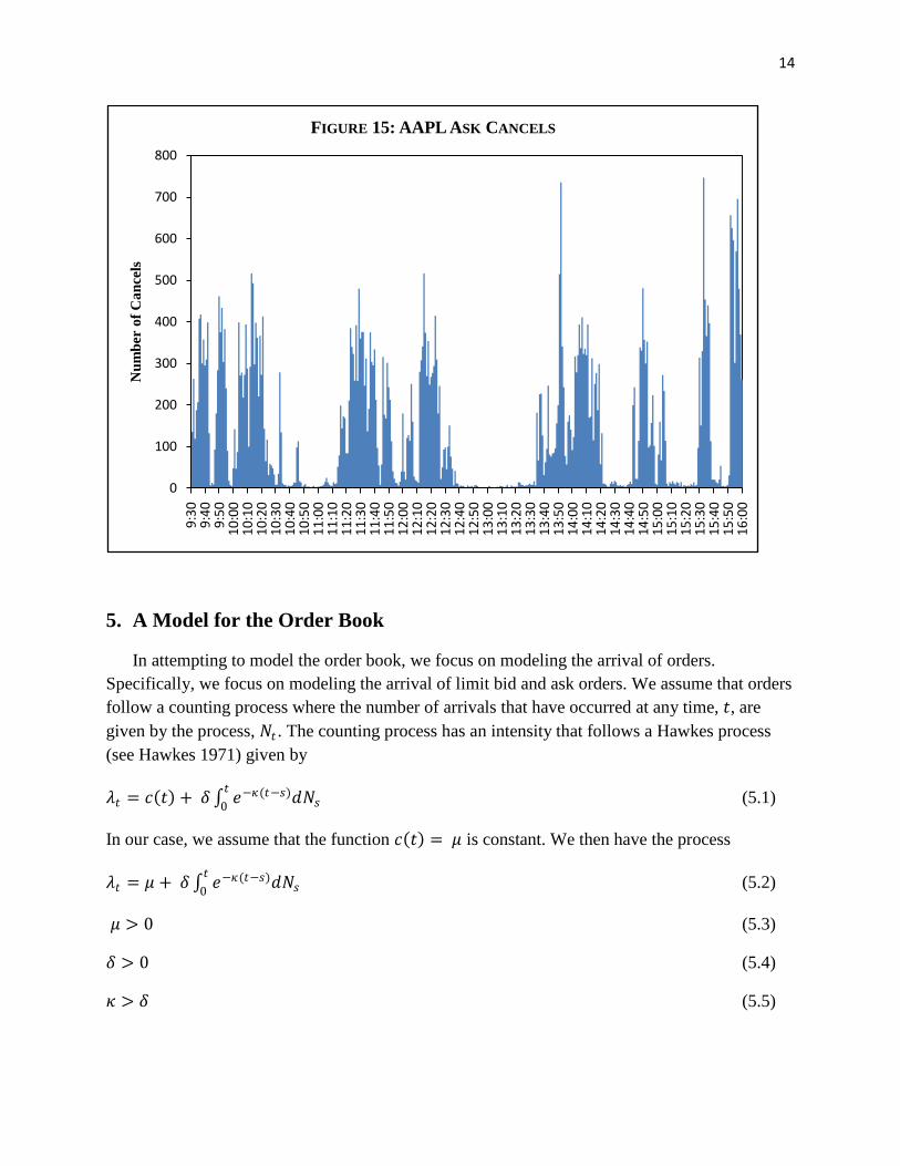
Figures 14 and 15 display the arrival of ask cancellations. For the sake of brevity, we exclude the arrival of bid cancellations but they follow a similar pattern. High periods of cancellation activity are typically followed by periods of dramatic price movements. This can be verified by examining the beginning of the trading day for QQQQ. Prices rose dramatically at the open when ask cancellations were high. As prices moved higher, it was likely that high frequency traders cancelled their sell orders and waited for the market to settle. If they were not to cancel, they might have found themselves selling into a rising market, a strategy which, when holding periods are only a few seconds, leads to losses.
0
2000
4000
6000
8000
10000
12000
14000
16000
9:30
9:40
9:50
10:0
010
:10
10:2
010
:30
10:4
010
:50
11:0
011
:10
11:2
011
:30
11:4
011
:50
12:0
012
:10
12:2
012
:30
12:4
012
:50
13:0
013
:10
13:2
013
:30
13:4
013
:50
14:0
014
:10
14:2
014
:30
14:4
014
:50
15:0
015
:10
15:2
015
:30
15:4
015
:50
16:0
0
Num
ber
of O
rder
s
FIGURE 10: QQQQ MARKET BUY ORDERS
12
0
2000
4000
6000
8000
10000
12000
14000
25.20
25.40
25.60
25.80
26.00
26.20
26.40
26.60
26.80
9:30
10:0
0
10:3
0
11:0
0
11:3
0
12:0
0
12:3
0
13:0
0
13:3
0
14:0
0
14:3
0
15:0
0
15:3
0
16:0
0
Num
ber of Orders
Mid
Quo
teFIGURE 11: QQQQ MARKET SELL ORDERS AND PRICE
0
500
1000
1500
2000
2500
3000
3500
4000
4500
5000
80.00
81.00
82.00
83.00
84.00
85.00
86.00
87.00
88.00
9:30
10:0
0
10:3
0
11:0
0
11:3
0
12:0
0
12:3
0
13:0
0
13:3
0
14:0
0
14:3
0
15:0
0
15:3
0
16:0
0
Num
ber of Order
Mid
Quo
te
FIGURE 12: AAPL MARKET BUY ORDERS AND PRICE
13
0
500
1000
1500
2000
2500
3000
3500
4000
4500
5000
9:30
9:40
9:50
10:0
010
:10
10:2
010
:30
10:4
010
:50
11:0
011
:10
11:2
011
:30
11:4
011
:50
12:0
012
:10
12:2
012
:30
12:4
012
:50
13:0
013
:10
13:2
013
:30
13:4
013
:50
14:0
014
:10
14:2
014
:30
14:4
014
:50
15:0
015
:10
15:2
015
:30
15:4
015
:50
16:0
0
Num
ber
of O
rder
sFIGURE 13: AAPL MARKET SELL ORDERS
0
500
1000
1500
2000
2500
9:30
9:40
9:50
10:0
010
:10
10:2
010
:30
10:4
010
:50
11:0
011
:10
11:2
011
:30
11:4
011
:50
12:0
012
:10
12:2
012
:30
12:4
012
:50
13:0
013
:10
13:2
013
:30
13:4
013
:50
14:0
014
:10
14:2
014
:30
14:4
014
:50
15:0
015
:10
15:2
015
:30
15:4
015
:50
16:0
0
Num
ber
of C
ance
ls
FIGURE 14: QQQQ ASK CANCELS
14
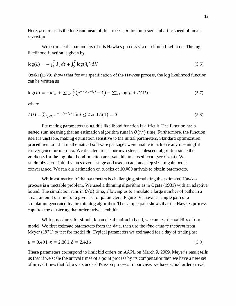
5. A Model for the Order Book
In attempting to model the order book, we focus on modeling the arrival of orders. Specifically, we focus on modeling the arrival of limit bid and ask orders. We assume that orders follow a counting process where the number of arrivals that have occurred at any time, 𝑡𝑡, are given by the process, 𝑁𝑁𝑡𝑡 . The counting process has an intensity that follows a Hawkes process (see Hawkes 1971) given by
𝜆𝜆𝑡𝑡 = 𝑐𝑐(𝑡𝑡) + 𝛿𝛿 ∫ 𝑒𝑒−𝜅𝜅(𝑡𝑡−𝑠𝑠)𝑑𝑑𝑁𝑁𝑠𝑠𝑡𝑡
0 (5.1)
In our case, we assume that the function 𝑐𝑐(𝑡𝑡) = 𝜇𝜇 is constant. We then have the process
𝜆𝜆𝑡𝑡 = 𝜇𝜇 + 𝛿𝛿 ∫ 𝑒𝑒−𝜅𝜅(𝑡𝑡−𝑠𝑠)𝑑𝑑𝑁𝑁𝑠𝑠𝑡𝑡
0 (5.2)
𝜇𝜇 > 0 (5.3)
𝛿𝛿 > 0 (5.4)
𝜅𝜅 > 𝛿𝛿 (5.5)
0
100
200
300
400
500
600
700
800
9:30
9:40
9:50
10:0
010
:10
10:2
010
:30
10:4
010
:50
11:0
011
:10
11:2
011
:30
11:4
011
:50
12:0
012
:10
12:2
012
:30
12:4
012
:50
13:0
013
:10
13:2
013
:30
13:4
013
:50
14:0
014
:10
14:2
014
:30
14:4
014
:50
15:0
015
:10
15:2
015
:30
15:4
015
:50
16:0
0
Num
ber
of C
ance
lsFIGURE 15: AAPL ASK CANCELS
15
Here, 𝜇𝜇 represents the long run mean of the process, 𝛿𝛿 the jump size and 𝜅𝜅 the speed of mean reversion.
We estimate the parameters of this Hawkes process via maximum likelihood. The log likelihood function is given by
log(𝐿𝐿) = −∫ 𝜆𝜆𝑡𝑡𝑇𝑇
0 𝑑𝑑𝑡𝑡 + ∫ log(𝜆𝜆𝑡𝑡)𝑑𝑑𝑁𝑁𝑡𝑡𝑇𝑇
0 (5.6)
Ozaki (1979) shows that for our specification of the Hawkes process, the log likelihood function can be written as
log(𝐿𝐿) = −𝜇𝜇𝑡𝑡𝑛𝑛 + ∑ 𝛿𝛿𝜅𝜅�𝑒𝑒−𝜅𝜅(𝑡𝑡𝑛𝑛−𝑡𝑡𝑖𝑖) − 1� + ∑ log{𝜇𝜇 + 𝛿𝛿𝛿𝛿(𝑖𝑖)}𝑛𝑛
𝑖𝑖=1𝑛𝑛𝑖𝑖=1 (5.7)
where
𝛿𝛿(𝑖𝑖) = ∑ 𝑒𝑒−𝜅𝜅(𝑡𝑡𝑖𝑖−𝑡𝑡𝑗𝑗 )𝑡𝑡𝑗𝑗<𝑡𝑡𝑖𝑖 for 𝑖𝑖 ≤ 2 and 𝛿𝛿(1) = 0 (5.8)
Estimating parameters using this likelihood function is difficult. The function has a nested sum meaning that an estimation algorithm runs in 𝑂𝑂(𝑛𝑛2) time. Furthermore, the function itself is unstable, making estimation sensitive to the initial parameters. Standard optimization procedures found in mathematical software packages were unable to achieve any meaningful convergence for our data. We decided to use our own steepest descent algorithm since the gradients for the log likelihood function are available in closed form (see Ozaki). We randomized our initial values over a range and used an adapted step size to gain better convergence. We ran our estimation on blocks of 10,000 arrivals to obtain parameters.
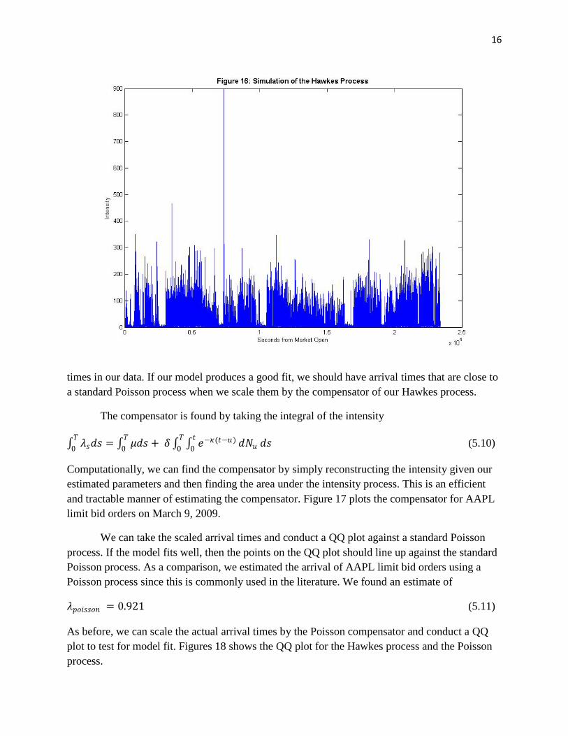
While estimation of the parameters is challenging, simulating the estimated Hawkes process is a tractable problem. We used a thinning algorithm as in Ogata (1981) with an adaptive bound. The simulation runs in 𝑂𝑂(𝑛𝑛) time, allowing us to simulate a large number of paths in a small amount of time for a given set of parameters. Figure 16 shows a sample path of a simulation generated by the thinning algorithm. The sample path shows that the Hawkes process captures the clustering that order arrivals exhibit.
With procedures for simulation and estimation in hand, we can test the validity of our model. We first estimate parameters from the data, then use the time change theorem from Meyer (1971) to test for model fit. Typical parameters we estimated for a day of trading are
𝜇𝜇 = 0.491, 𝜅𝜅 = 2.801, 𝛿𝛿 = 2.436 (5.9)
These parameters correspond to limit bid orders on AAPL on March 9, 2009. Meyer’s result tells us that if we scale the arrival times of a point process by its compensator then we have a new set of arrival times that follow a standard Poisson process. In our case, we have actual order arrival
16
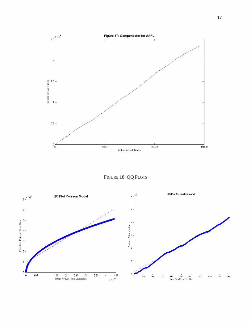
times in our data. If our model produces a good fit, we should have arrival times that are close to a standard Poisson process when we scale them by the compensator of our Hawkes process.
The compensator is found by taking the integral of the intensity
∫ 𝜆𝜆𝑠𝑠𝑑𝑑𝑠𝑠 = ∫ 𝜇𝜇𝑑𝑑𝑠𝑠𝑇𝑇0
𝑇𝑇0 + 𝛿𝛿 ∫ ∫ 𝑒𝑒−𝜅𝜅(𝑡𝑡−𝑢𝑢)𝑡𝑡
0 𝑑𝑑𝑁𝑁𝑢𝑢𝑇𝑇
0 𝑑𝑑𝑠𝑠 (5.10)
Computationally, we can find the compensator by simply reconstructing the intensity given our estimated parameters and then finding the area under the intensity process. This is an efficient and tractable manner of estimating the compensator. Figure 17 plots the compensator for AAPL limit bid orders on March 9, 2009.
We can take the scaled arrival times and conduct a QQ plot against a standard Poisson process. If the model fits well, then the points on the QQ plot should line up against the standard Poisson process. As a comparison, we estimated the arrival of AAPL limit bid orders using a Poisson process since this is commonly used in the literature. We found an estimate of
𝜆𝜆𝑝𝑝𝑝𝑝𝑖𝑖𝑠𝑠𝑠𝑠𝑝𝑝𝑛𝑛 = 0.921 (5.11)
As before, we can scale the actual arrival times by the Poisson compensator and conduct a QQ plot to test for model fit. Figures 18 shows the QQ plot for the Hawkes process and the Poisson process.
17
FIGURE 18: QQ PLOTS

18
Clearly, the Hawkes process is a much better fit than the Poisson process. This is to be expected since the Poisson process assumes a constant arrival time between orders and, therefore, fails to capture any notion of clustering. The Hawkes process deviates most from the data when there are few orders in a period of time. In other words, it struggles to capture the periods of inactivity that were seen in order arrival data. We suggest a possible improvement to this drawback in our conclusion.
6. Application to High Frequency Trading
One of the applications of our model is high frequency trading. A successful high frequency trading strategy relies on one’s ability to predict price movements over a short period of time. We showed earlier that the arrival of limit bid and ask orders are an excellent predictor of short term price movements. It follows that a model that can effectively predict the arrival of limit bid and ask orders can be used to formulate successful high frequency trading strategies.
The framework for our trading strategy is as follows: we estimate parameters from a block of data. We simulate order arrivals based on these parameters. We then institute triggers based on the simulated intensity which would cause an algorithm to go long or short the stock. We tested this strategy, varying our triggers and our holding time. Assuming no transaction costs, no restrictions on shorting, a two second holding period and single unit per trade, we made an average profit of $0.0003 per trade. Figure19 displays a simulated intensity path overlaid with AAPL mid-quote for March 9, 2009.
FIGURE 19: HIGH FREQUENCY TRADING
19
We faced several issues when implementing this strategy. Foremost among them was estimating the parameters. As was discussed in the previous section, the maximum likelihood function is slow to estimate and unstable. Speed is of particular relevance in our case because we need to estimate parameters quickly so that we can make trades while our parameters are still relevant. If our estimation procedure takes too long then we will not have the opportunity to trade no matter how accurate our parameter estimates. Ultimately, we decided to estimate our parameters on a rolling 10,000 trade window. This worked well for AAPL but was not as effective for QQQQ because QQQQ is so active.
The second problem we faced is inherent to the testing of trading strategies. We are never able to take into account our own effect on the market; we can simply back test on existing data. As a result, we can never be sure that the market will react in the same manner when we actually trade. To counter this problem, we fixed our trade size at 1 unit. We assumed that trading in such small quantities would have minimal effects on the market, especially in active stocks such as QQQQ and AAPL. In addition, we constructed our own trading simulator to get accurate back testing results. The advantage of doing this was that we could reconstruct the order book as before but now with trades made by our algorithm. This allowed us to effectively track our algorithm’s trading and simulate a more realistic environment for testing.
7. Conclusion
In studying the empirical properties of the order book, we found that properties governing the arrival of orders were critical in determining price dynamics. We showed that order arrivals exhibit clustering and lend themselves to a self-exciting point process model. We used a Hawkes process to model the arrival of limit orders and showed that our model fit the data better than the much used Poisson model.
We applied our Hawkes process model to high frequency trading. While our model was relatively successful we faced several difficulties and found areas for further work. Much of this work should focus on better estimation procedures for the Hawkes process likelihood function. Quicker estimation and better convergence will make the model significantly more useful. It will allow the model to be applied to the trading of more active stocks, trading at a higher frequency and, perhaps, trading with better signals due to more accurate parameter estimates.
Future research should also look to improve the Hawkes process we implemented. Order arrival data is characterized by flurries of orders and periods of inactivity. While our model was effective in capturing the high activity periods, it failed to capture lulls in trading. A possible extension to the model that might capture low activity periods is a regime dependent model. By this, we mean a model that has parameters that depend on the intensity. In this case, low intensity periods will correspond to a “low regime” and periods of inactivity can be sustained. We believe that trading strategies based on this type of model will not only be successful for the types of stock we studied in this paper but extend further and find applications in more illiquid names.
20
References
Alfonsi, A., A. Schied, A. Schulz. 2007. Optimal execution strategies in limit order books with general shape functions. Working paper. Biais, B., P. Hilton, C. Spatt. 1995. An empirical analysis of the limit order book and the order flow in the Paris Bourse, Journal of Finance, 50, pp. 1655-89 Bouchaud, J., M. M´ezard, M. Potters. 2002. Statistical properties of stock order books: empirical results and models. Quantitative Finance, 2, pp. 251–256. Foucault, T., O. Kadan, E. Kandel. 2005. Limit order book as a market for liquidity. Review of Financial Studies, 18(4), pp. 1171–1217. Harris, L. Trading & Exchanges: Market Microstructure for Practitioners. 2003. New York, NY: Oxford University Press, New York. Hawkes, A. 1971. Spectral of some self-exciting and mutually exciting point processes. Biometrika, 58(1), pp. 83-90. Hewlett, P. 2006. Clustering of order arrivals, price impact and trade path optimization. Workshop on Financial Modeling with Jump processes, Ecole Polytechnique, 6–8 September 2006. Meyer, P. 1971. Demonstration simplifiée d’un théorème de Knight. In Séminaire de Probabilités V, Univ. Strasbourg, Lecture Notes in Math. 191, pp. 191–195. Obizhaeva, A., J. Wang. 2006. Optimal trading strategy and supply/demand dynamics. Working paper, MIT. Ogata, Y. 1981. On Lewis’s Simulation Method for Point Processes, IEEE Transactions on Information Theory, IT-27(1). Smith, E., J. D. Farmer, L. Gillemot, S. Krishnamurthy. 2003. Statistical theory of the continuous double auction. Quantitative Finance 3(6), pp. 481–514.