1

Recommendations Using Information from Multiple Association Rules: A Probabilistic Approach

Abstract

Business analytics has evolved from being a novelty used by a select few, to an accepted facet of conducting business. Recommender systems form a critical component of the business analytics toolkit and, by enabling firms to effectively target customers with products and services, are helping alter the e-commerce landscape. A variety of methods exist for providing recommendations, with collaborative filtering, matrix factorization, and association rule based methods being the most common. In this paper, we propose a method to improve the quality of recommendations made using association rules. This is accomplished by combining rules when possible, and stands apart from existing rule-combination methods in that it is strongly grounded in probability theory. Combining rules requires the identification of the best combination of rules from the many combinations that might exist, and we use a maximum-likelihood framework to compare alternative combinations. As it is impractical to apply the maximum likelihood framework directly in real time, we show that this problem can equivalently be represented as a set partitioning problem by translating it into an information theoretic context – the best solution corresponds to the set of rules that leads to the highest sum of mutual information associated with the rules. Through a variety of experiments that evaluate the quality of recommendations made using the proposed approach, we show that (i) a greedy heuristic used to solve the maximum likelihood estimation problem is very effective, providing results comparable to those from using the optimal set partitioning solution, (ii) the recommendations made by our approach are more accurate than those made by a variety of state-of-the-art benchmarks, including collaborative filtering and matrix factorization, and (iii) the recommendations can be made in a fraction of a second on a desktop computer, making it practical to use in real-world applications.

Keywords: Personalization, Bayesian Estimation, Maximum Likelihood, Information Theory

1. Introduction

A recent International Data Corporation (IDC) report estimates that the business analytics market will

grow at a compounded rate of 9.8%, and reach 50.7 billion by 2016. This is partly fueled by the growth in

the amount of customer data readily available to firms, and the potential for businesses to leverage their

data through the novel use of software-based analytic techniques. Recommender systems form an integral

part of the business analytics toolkit, and several studies have shown that personalized recommendations

can enable firms to effectively target customers with products and services (Häubl and Trifts 2000, Tam

and Ho 2003). For example, Pathak et al. (2010) find that the strength of a recommender system has a

positive effect on sales and on prices.

Recommendations are made on a continuous basis, and can have a substantial impact on the

bottom line. According to Hosanagar et al. (2012), 60% of Netflix rentals stem from recommendations,

while 35% of Amazon’s sales originate from their recommendation system. It is easy to see that even a

2

small improvement in the quality of recommendations would be worth millions of dollars every year to a

retailer.

A variety of methods exist for providing recommendations, with collaborative filtering, matrix

factorization, and association rule based methods being the most common. In this paper, we focus on

improving the quality of rule based recommendations by combining information from multiple

association rules. Rule-based approaches comprise one prominent class of techniques used to provide

personalized recommendations to customers. Firms such as BroadVision have emerged that provide rule-

based tools to firms that wish to implement recommendation systems on their web sites (Hanson 2000).

Rules are easy to understand, which appeals to marketers interested in cross-selling or product placement.

Often, such rule based systems use association rules (Hastie et al. 2009).

Association rules are implications of the form {bread, milk}→ {yogurt}, where {bread, milk} is

called the antecedent of the rule and {yogurt} is called its consequent. While millions of such

implications are possible in a typical dataset, not all of them are useful for providing recommendations.

Agrawal et al. (1993) provided a method to identify those rules where the items in the rules appear in a

reasonably large numbers of transactions (termed the support of the rule), and where a consequent has a

high probability of being chosen when the items in the antecedent have already been chosen (termed the

confidence of the rule). Every mined rule must meet minimum thresholds for both support and

confidence.

Association rules compactly express how products group together (Berry and Linoff 2004), and

have been successfully used for market basket analysis (Gordon 2008, Lewin 2009). Recommendation

systems based on association rules leverage available rules and a customer’s basket, to recommend items

as the customer is shopping. Many firms implement association rule based recommender systems as they

can be used unobtrusively in automated systems to provide recommendations to customers in real time.

For instance, Forsblom et al. (2009) develop a mobile application for a Nokia smartphone that uses

association rules to recommend retail products to customers. Prominent companies like IBM promote

association rule mining capabilities in their business analytics software (IBM 2009a, 2009b, 2010).

While there has been considerable work done on mining rules more efficiently (e.g., Ng. et al.

1998, Bayardo and Agrawal 1999, Zaki 2000), research into the use of rules to make effective

recommendations is scarce. Zaïane (2002) proposed a method that finds all eligible rules (rules whose

antecedents are subsets of the basket and whose consequents are not), and recommends the consequent of

the eligible rule with the highest confidence. Wang and Shao (2004) suggest considering only maximal

3

rules, i.e., eligible rules whose antecedents are maximal-matching1 subsets of the basket. Both these

approaches focus on identifying a single rule to make the recommendation. Often however, the antecedent

of the selected rule will not contain all the items in the basket. Consequently, the recommendation is

made on the basis of partial information – items not present in the antecedent of the rule being used for

recommendation are effectively ignored. It is not difficult to see that the item being recommended could

be different had the recommendation system been able to use information from all the items in the basket.

The set of eligible rules often contains multiple rules with the same consequent, and the quality of

recommendations could potentially be improved by combining such rules effectively.

The notion of combining rules has been explored in a few studies in the past. Given a customer’s

basket, Lin et al. (2002) calculate the score for each item as the sum of the products of the supports and

confidences of all eligible rules with this item as the consequent. The item with highest score is

recommended to the customer. Wickramaratna et al. (2009) present an approach to identify rules that

predict the presence and absence of an item, and propose a Dempster-Shaffer based approach for

combining rules when some rules predict that a customer will purchase an item, while other rules predict

the contrary. However they note that their approach is not scalable for real-time applications.

There has also been some work that attempts to combine classification rules. Li et al. (2001)

suggest classifying customers using Classification based on Multiple Association Rules (CMAR). They

group eligible rules with the same consequent (class), and evaluate the sum of weighted chi-squares of the

rules in each group. The customer is assigned to the consequent class corresponding to the group with the

highest sum. Liu et al. (2003) classify customers using a score calculated based on the combination of all

the eligible rules (determined based on the attributes of the customer). Their scoring formula requires the

identification of rules with negations and cannot be adapted for selecting items to recommend in a

traditional association rule mining context.

Two other techniques that have been successfully employed in recommendation systems are

collaborative filtering and matrix factorization. Collaborative filtering based methods are perhaps the best

known, at least since Amazon.com decided to deploy it as part of their recommender system (Linden et al.

2003). These methods use the known preferences of a group of users to make recommendations or

predictions of the unknown preferences for other users. Matrix factorization methods gained recognition

partly as a result of successes in the Netflix Prize competition. These methods represent users and items

through factors identified from the data, and an item is recommended to a user when the item and user are

similar vis-à-vis these factors (Koren et al. 2009).

1 An antecedent is maximal matching if no supersets of it, present as antecedents of other rules, are subsets of the basket.

4

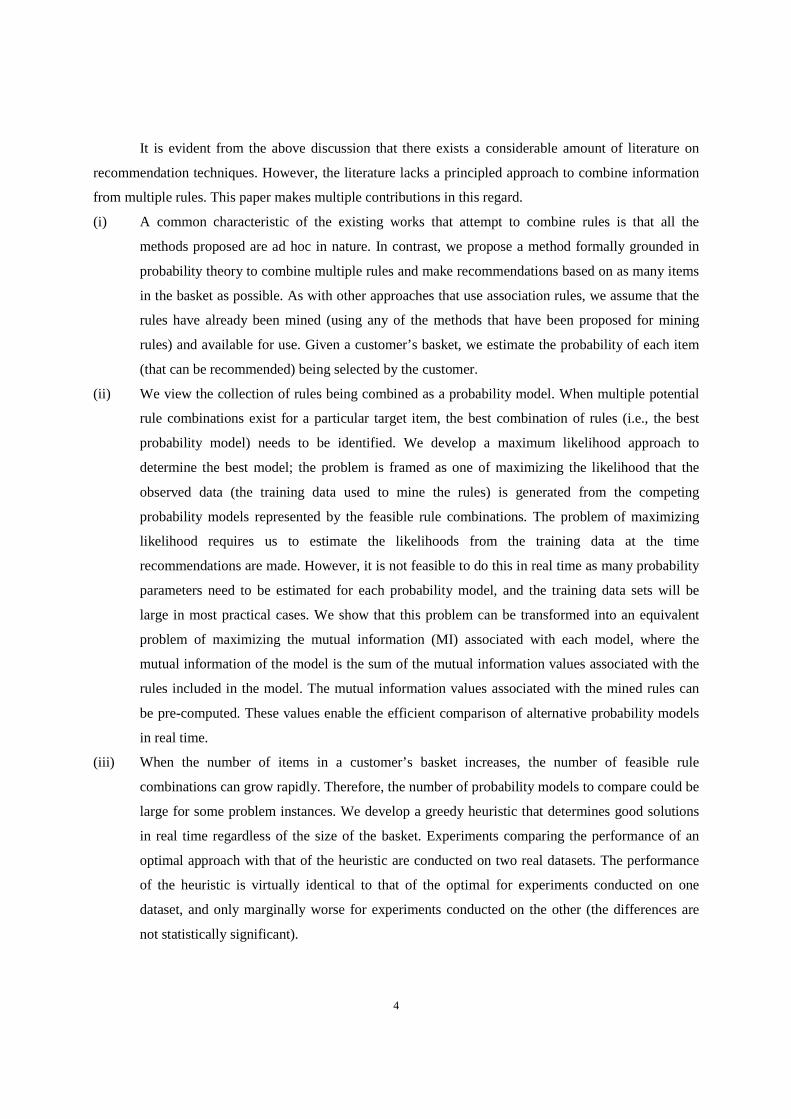
It is evident from the above discussion that there exists a considerable amount of literature on

recommendation techniques. However, the literature lacks a principled approach to combine information

from multiple rules. This paper makes multiple contributions in this regard.

(i) A common characteristic of the existing works that attempt to combine rules is that all the

methods proposed are ad hoc in nature. In contrast, we propose a method formally grounded in

probability theory to combine multiple rules and make recommendations based on as many items

in the basket as possible. As with other approaches that use association rules, we assume that the

rules have already been mined (using any of the methods that have been proposed for mining

rules) and available for use. Given a customer’s basket, we estimate the probability of each item

(that can be recommended) being selected by the customer.

(ii) We view the collection of rules being combined as a probability model. When multiple potential

rule combinations exist for a particular target item, the best combination of rules (i.e., the best

probability model) needs to be identified. We develop a maximum likelihood approach to

determine the best model; the problem is framed as one of maximizing the likelihood that the

observed data (the training data used to mine the rules) is generated from the competing

probability models represented by the feasible rule combinations. The problem of maximizing

likelihood requires us to estimate the likelihoods from the training data at the time

recommendations are made. However, it is not feasible to do this in real time as many probability

parameters need to be estimated for each probability model, and the training data sets will be

large in most practical cases. We show that this problem can be transformed into an equivalent

problem of maximizing the mutual information (MI) associated with each model, where the

mutual information of the model is the sum of the mutual information values associated with the

rules included in the model. The mutual information values associated with the mined rules can

be pre-computed. These values enable the efficient comparison of alternative probability models

in real time.

(iii) When the number of items in a customer’s basket increases, the number of feasible rule

combinations can grow rapidly. Therefore, the number of probability models to compare could be

large for some problem instances. We develop a greedy heuristic that determines good solutions

in real time regardless of the size of the basket. Experiments comparing the performance of an

optimal approach with that of the heuristic are conducted on two real datasets. The performance

of the heuristic is virtually identical to that of the optimal for experiments conducted on one

dataset, and only marginally worse for experiments conducted on the other (the differences are

not statistically significant).

5

(iv) The effectiveness of our methodology – termed Maximum Likelihood Recommendations (MLR) –

is demonstrated through a variety of additional computational experiments that compare it to

many key benchmarks. We compare the accuracy of recommendations made by MLR to those

made by (a) the single rule approaches of Zaïane (2002) and Wang and Shao (2004), (b) the rule

combination approaches of Li et al. (2001) and Lin et al. (2002), (c) item-based collaborative

filtering, and (d) matrix factorization (FunkSVD). MLR is shown to outperform all the

benchmarks, and the performance improvements are observed to be robust at various support and

confidence thresholds used for mining rules in both datasets. When it is feasible to combine

multiple rules so that a larger proportion of the basket is covered by the rule antecedents than

would be possible otherwise, MLR performs particularly well.

We describe the problem in detail in Section 2, while the methodology is discussed in Section 3.

Section 4 presents results of the experiments conducted to validate our approach for rule-based

recommendation environments. Section 5 compares MLR with the collaborative filtering and matrix

factorization approaches. Section 6 concludes the paper.

2. Problem Description

The problem being considered in this paper is best illustrated through an example. Consider a customer

who has three items i1, i2, and i3 in her basket B, i.e., B = { i1, i2, i3}. The eligible rules for this basket – i.e.,

all available rules whose antecedents are subsets of the basket – are listed in Table 1. Rules R1 – R4 have

item x1 as their consequent, while item x2 is the consequent of rules R5 – R8. Our task is to select one of x1

or x2 and recommend it to the customer.

Rule Antecedent Consequent Confidence

R1 i1,i2 x1 60% R2 i2,i3 x1 40% R3 i1 x1 54% R4 i3 x1 45% R5 i1,i3 x2 42% R6 i2,i3 x2 50% R7 i1 x2 58% R8 i2 x2 62%

Table 1: Eligible rules for basket B = { i1,i2,i3} Traditional rule based approaches identify the best rule from the eligible set, and recommends the

associated consequent. So, for example, Zaïane’s (2002) approach would rank the eligible rules based on

their confidences, and select the consequent of the rule with the highest confidence as the item to

recommend. The rule with the highest confidence in our example is R8, and consequently, x2 would be

6

recommended to the customer. However, recommending x2 based on R8 ignores some items in the basket

(i1 and i3), despite the fact that another rule – R5 – exists with these items in the antecedent. This is true in

general – making a recommendation based on a single rule often disregards items in the basket that are

not in the antecedent of the rule being used.

If we could effectively combine rules and cover as many items of the basket as possible, our

recommendation would be more informed. The question then becomes one of identifying the best way to

combine multiple rules. This is the primary objective of this paper – to provide a theoretical basis for

combining rules. Given the items in a customer’s basket, we combine rules when necessary to estimate

the probabilities of each relevant consequent being selected by the customer, and recommend the item

with the highest probability. Note that this is not unlike what the single rule approach would do, had there

been a rule whose antecedent covered the entire basket – i.e., combinations of rules can be interpreted in

much the same way as any single rule would be.

Before we calculate the probabilities associated with each potential recommendation however, we

need to identify the rules to combine. It is quite possible that there will be multiple potential combinations

to choose from. For example, we have already seen that rules R5 and R8 could be combined to estimate the

probability for x2. From Table 1, we can also see that rules R6 and R7 could be used to estimate the same

probability as well. Different combinations of rules can yield different probability estimates, and we show

how to choose the best combination from the different alternatives.

3. MLR: Maximum Likelihood Recommendations

MLR can be viewed as a three step process. The first step identifies all the eligible rules and from them,

the feasible consequents. For each of these feasible consequents, the best probability estimate conditioned

on the basket is identified in the second step. The third step selects the consequent with the highest

probability.

3.1 Identifying Eligible Rules and Consequents

We first find all the eligible rules by ensuring that all items in the antecedent of a selected rule appear in

the basket while its consequent does not. The consequents of the eligible rules are added to a consequent

list M. In our example, M contains two consequents {x1, x2}.

3.2 Computing the Probability of a Consequent

Given a customer with a basket B, we are interested in estimating P(x | B), the probability that she will

choose item x from M. While we would ideally like to use a rule that has x as the consequent and an

antecedent identical to B, such a rule may not exist. It is more likely that we will find several rules with x

7

as the consequent, whose antecedents are subsets of B. These rules can be used, with appropriate

conditional independence assumptions, to arrive at an estimate for P(x | B). Such assumptions have been

extensively used for estimation when the available data are not sufficient to estimate the full distributions,

and have been found to be robust in practice (Domingos and Pazzani 1997).2

Specifically, if we have multiple eligible rules with disjoint antecedents and a common

consequent x, we can estimate P(x | B) by combining the information in these rules under the assumption

that the antecedents are conditionally independent given the common consequent x. Note that the

antecedents of the rules being combined have to be disjoint to avoid double counting the impact of the

common items in the rules.

Suppose there are r eligible rules with disjoint antecedents that have x as the consequent. Let the

antecedent of rule Rj be Aj and let A represent⋃ ������ . By assuming that the antecedents Aj are

conditionally independent given x, we can approximate P(x | B) as P(x | A) below.

P(x | A)= �| �∗ ��� = �| �∗ �

,��� ̅,�� = ∏ ���� ��∗ �����∏ ���� ��∗ ����� �∏ ���� ̅��∗ ̅����� (1)

In order to evaluate P(x | A) using (1), we need to know P(x) and P(�̅), along with P(Aj | x) and P(Aj | �̅)

for each of the r rules Rj. P(x) is simply the support of the consequent x, while P(�̅) is (1 - P(x)). Each of

the parameters P(Aj | x) and P(Aj | �̅) can be obtained from the confidences of the rules involved (i.e., P(x |

Aj)), and the supports of x and Aj (i.e., P(x) and P(Aj)). All these parameters can be pre-computed from the

data at the time the rules are mined.

Consider using rules R1 and R4 from the example in Table 1, to compute P(x1 | B) for consequent

x1. Assume that P(x1) = 0.2, P(A1) = 0.3, and P(A4) = 0.2, for our illustrative example. Using these

probabilities and the confidences of the two rules, the additional parameters required in (1) can be

calculated as:

��̅�� = 1 − ���� = 0.8,

���|��� = �|���∗��� �� = 0.9, ���|�̅�� = ���# �|���∗���

�# ��� = 0.15,

2 To examine the implications of making conditional independence assumptions, we conducted experiments where we estimated directly from the data the probabilities associated with all feasible consequents given the entire basket (so that conditional independence assumptions are not needed). The recommendations from using such estimates were much worse compared to when rules are combined with appropriate conditional independence assumptions. This is because the number of transactions that support the entire basket reduces drastically as the size of the basket grows, and the estimates when considering the full baskets become less reliable.

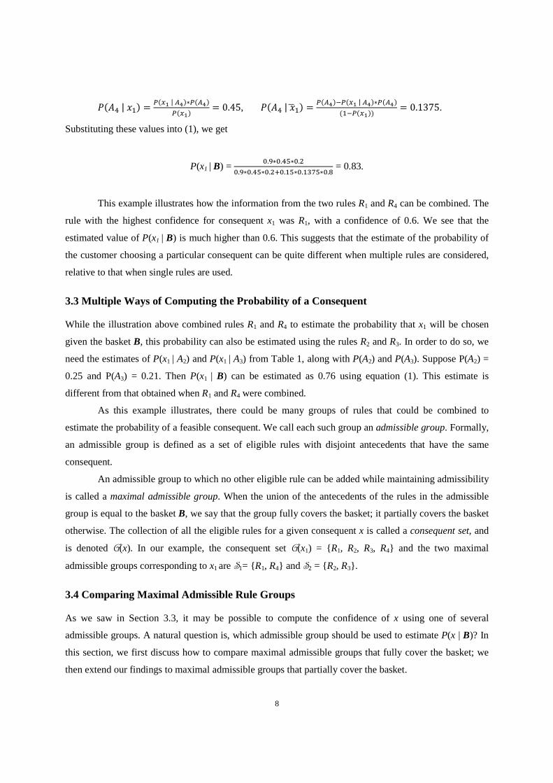
8

��%|��� = �|�&�∗�&� �� = 0.45, ��%|�(�� = �&�# �|�&�∗�&�

�# ��� = 0.1375.

Substituting these values into (1), we get

P(x1 | B) = +.,∗+.%-∗+..

+.,∗+.%-∗+..�+.�-∗+.�/0-∗+.1 = 0.83.

This example illustrates how the information from the two rules R1 and R4 can be combined. The

rule with the highest confidence for consequent x1 was R1, with a confidence of 0.6. We see that the

estimated value of P(x1 | B) is much higher than 0.6. This suggests that the estimate of the probability of

the customer choosing a particular consequent can be quite different when multiple rules are considered,

relative to that when single rules are used.

3.3 Multiple Ways of Computing the Probability of a Consequent

While the illustration above combined rules R1 and R4 to estimate the probability that x1 will be chosen

given the basket B, this probability can also be estimated using the rules R2 and R3. In order to do so, we

need the estimates of P(x1 | A2) and P(x1 | A3) from Table 1, along with P(A2) and P(A3). Suppose P(A2) =

0.25 and P(A3) = 0.21. Then P(x1 | B) can be estimated as 0.76 using equation (1). This estimate is

different from that obtained when R1 and R4 were combined.

As this example illustrates, there could be many groups of rules that could be combined to

estimate the probability of a feasible consequent. We call each such group an admissible group. Formally,

an admissible group is defined as a set of eligible rules with disjoint antecedents that have the same

consequent.

An admissible group to which no other eligible rule can be added while maintaining admissibility

is called a maximal admissible group. When the union of the antecedents of the rules in the admissible

group is equal to the basket B, we say that the group fully covers the basket; it partially covers the basket

otherwise. The collection of all the eligible rules for a given consequent x is called a consequent set, and

is denoted G(x). In our example, the consequent set G(x1) = {R1, R2, R3, R4} and the two maximal

admissible groups corresponding to x1 are S1= {R1, R4} and S2 = {R2, R3}.

3.4 Comparing Maximal Admissible Rule Groups

As we saw in Section 3.3, it may be possible to compute the confidence of x using one of several

admissible groups. A natural question is, which admissible group should be used to estimate P(x | B)? In

this section, we first discuss how to compare maximal admissible groups that fully cover the basket; we

then extend our findings to maximal admissible groups that partially cover the basket.

9

Ideally, we should use that admissible group which can best approximate the true joint

distribution across the items in the basket B and x, i.e., P(B, x). Therefore, we compare the admissible

groups using the likelihood of each group generating the true underlying distribution P(B, x). The

likelihoods of interest in our case are those associated with the probability models implied by the

collection of rules for each admissible group. Specifically, each admissible group corresponds to a

probability model with some associated conditional independence assumptions. For example, the

admissible group S1 = {R1, R4} assumes that the set {i1, i2} is conditionally independent of the set {i3}

given x1, while S2 = {R2, R3} assumes that the set {i2, i3} is conditionally independent of the set {i1} given

x1. Therefore, by comparing the admissible groups using their likelihoods, we are essentially checking

which conditional independence assumption is most likely to hold, given the data. In essence, this

problem can be viewed as one of maximizing the likelihood that the observed data is generated from the

competing probability models represented by the admissible groups.

The maximum-likelihood framework requires the estimation of the likelihoods from training data.

This is not feasible in real time as training data sets can be large, and many parameters need to be

estimated for each probability model. Consequently, for this to be a useful approach, we have to

transform this into a problem that can be solved in real time. We show that the log-likelihood can be

conveniently represented as a function of the mutual information associated with the rules in an

admissible group, and the entropies of the items in the basket. The mutual information terms can be pre-

computed for every rule and kept available for use at run-time, which eliminates the need to estimate

parameters from the data during the recommendation process.

We define the mutual information associated with a rule to be the mutual information across all

the individual attributes in the rule (including the items in both the antecedent and the consequent of the

rule). Therefore, the mutual information (MI) across attributes i1, …, in is (Kullback 1959):

234�, … , 46� = 7 �4�, … , 46�log �4�, … , 46��4�� ∗. … ∗ �46�;�,…,;<

.

Thus, the mutual information associated with a rule Rj having antecedent Aj = { i j1,…, ijk} and

consequent xm is

MI(Rj) = MI(Aj, xm) = MI(i j1,…, ijk , xm) = ∑ �4��, … , 4�> , �?�log ;��,…,;�@, A��;��B∗.…∗�;�@B∗ A�;��,…,;�@, A .

The entropy of an item i is H(i) = − ∑ P4� log P4�D .

The mutual information associated with a rule captures the mutual dependency across all the

items in the antecedent and the consequent of the rule. The entropy of an attribute is a measure of how

much uncertainty is represented in the probability distribution of the attribute.

10

Proposition 1 below shows that the log-likelihood associated with a maximal admissible group

can be represented as the sum of the mutual information terms associated with each participating rule, less

the sum of the entropies associated with every item in the basket B and the entropy associated with the

consequent. Proposition 1 helps represent the problem using the mutual information terms associated with

rules. This has intuitive appeal, as the mutual information term for a rule is higher if the items in the

antecedent and the consequent are more dependent on each other. The best admissible group therefore, is

the one where the rules collectively convey as much information about the consequent as possible.

Proposition 1: Given a consequent and all corresponding admissible groups that fully cover the basket,

the admissible group that maximizes the likelihood also has the highest sum of the mutual information

terms associated with the participating rules.

Proof: We first show that the log-likelihood associated with a maximal admissible group can be

represented as the sum of the mutual information terms associated with each participating rule, less the

sum of the entropies associated with the consequent and all the items in the basket.

Given a basket B = { i1, …, in}, let the consequent of interest be in+1. To estimate the likelihood of

a probability model associated with an admissible group, we consider the distribution associated with

these items, based on the absence or presence of each item in every transaction of the data set. We denote

the binary attributes corresponding to the set of items as I = { i1, …, in, in+1}. Let the dataset T consist of s

transactions, i.e., T = {t1, t2,…, ts}, where tj is a vector of ones and zeros corresponding to the presence

and absence of the items i1,…, in+1 in the j th transaction.

Let there be r rules in an admissible group under consideration, and let Al denote the attributes

corresponding to the antecedent Al in the l th rule of the admissible group. The probability distribution

corresponding to the rules in the admissible group can be written as P(I) = ∏ ��E|FG�H��I�� ∗ �F6���.

The probability associated with the items appearing in the j th transaction, P(J�), is represented as

∏ ���I�|F6��� B ∗ ��F6��� B�I�� , and the likelihood for the admissible group is

K = ∏ ��J�BL��� = ∏ ∏ ��I�|F6��� ��I��L��� � ∗ �F6��� �.

The log-likelihood, L’ , is logK� = KM = ∑ ∑ log��I�|F6��� ��I��L��� + ∑ log�F6��� �L���

= ∑ ∑ log��I�|F6��� �L����I�� + ∑ log�F6��� �L��� . (2)

Each instance �I�, F6��� � corresponds to one of the 2(n+1) realizations of the attributes (i.e., the set of 0-1

values the attributes can assume) comprising the antecedent and the consequent of the l th rule. Let the

11

probability for the kth realization of �I, F6��� be�>�I , F6���. 3 Further, let the frequency of occurrences

for the kth realization of �I , F6��� beO>�I, FG���, and the frequency of occurrences for the kth realization

of in+1 be fk(in+1). Therefore,

∑ log���I��F6��� BL��� = ∑ O>�I , F6���log�>�I|F6���> , and

∑ log��F6��� BL��� = ∑ O>F6���log�>F6��> �.

Since �>�I , F6��� = P@�Q,F<R��L and �>F6��� = P@F<R��

L , we have

∑ log���I��F6��� BL��� = S ∑ P@�Q,F<R��L> log�>�I|F6��� = S ∑ �>�I, F6���log�>�I|F6���> .

Similarly, ∑ log��F6��� BL��� = S ∑ �>F6���log�>F6��> �.

Substituting for ∑ log���I��F6��� BL��� and ∑ log��F6��� BL��� in (2) we have,

KM = 7 S 7 �>�I, F6���log�>�I|F6���>

�I�� + S 7 �>F6���log�>F6��

>�

= S ∑ ∑ �>�I, F6���>�I�� log�>�I|F6��� + S ∑ �>F6���log�>F6��> � (3)

Consider the term ∑ �>�I , F6���log�>�I|F6���> in the first sum. Let the antecedent Al comprise of the

m items {i1,…,im}.

∑ �>�I , F6���log�>�I|F6���> = ∑ �>F�, F., … , F?, F6���log T@F�,FU,…,FA,F<R��@F<R�� V>

= ∑ �>F�, F., … , F?, F6���log T@F�,FU,…,FA,F<R��∗@F��∗…∗@FA�@F��∗…∗@FA�∗@F<R�� V>

= ∑ �>F�, F., … , F?, F6���log T @F�,FU,…,FA ,F<R��@F��∗…∗@FA�∗@F<R��V>

+ ∑ �>F�, F., … , F?, F6���log�>F�� ∗ … ∗ �>F?�> )

= ∑ �>F�, F., … , F?, F6���log T @F�,FU,…,FA ,F<R��@F��∗…∗@FA�∗@F<R��V> +

+ ∑ �>F�, F., … , F?, F6���log�>F��> + ⋯ + ∑ �>F�, F., … , F?, F6���log�>F?�>

Over all possible realizations of XF�, F., … , F? , F6��Y, ∑ �>F�, F., … , F? , F6���log�>�F�B> simplifies to

∑ �>�F�Blog�>�F�B> , with k now indexing all possible realizations ofZF�[, i.e., 0 and 1. Therefore,

7 �>�I, F6���log�>�I|F6���>

= 7 �>F�, F., … , F? , F6���log \ �>F�, F., … , F? , F6����>F�� ∗ … ∗ �>F?� ∗ �>FG�H�]

>

3 Depending on the number of items being considered in each distribution, the number of possible realizations will vary. Hence, the range for the index k will also vary. For notational simplicity, we do not spell out the range in the following expressions, implicitly assuming that k will vary over the appropriate range in each expression.

12

+ ∑ �>F��log�>F��> + ⋯ + ∑ �>F?�log�>F?�>

= 7 �>F�, F., … , F?, F6���log \ �>FH, F^, … , F_, F6����>F�� ∗ … ∗ �>F?� ∗ �>F6���]

>+ 7 7 �>�F`Blog�>�F`B>`a�E

= 23F�, F., … , F?, F6��� − ∑ b`�`a�E .

Therefore, by substituting for ∑ �>�I, F6���log�>�I|F6���> in (3) we get

KM = S ∑ 23I − S ∑ ∑ b`�`a�E�I�� − Sb6���I�� = S∑ 23I�I�� − ∑ b`�6��`�� ).

The entropy terms in the above expression are the same for every admissible group under consideration.

Therefore, the admissible group that maximizes the likelihood has the highest sum of mutual information

terms associated with the participating rules. ∎

The mutual information terms can be pre-computed for every rule and kept available for use at

run-time. Comparing admissible groups using mutual information is straightforward. For example,

suppose the mutual information values of the rules in S1 = {R1, R4} and S2 = { R2, R3} are as in Table 2.

Since the sum of the mutual information values for the rules in S1 (0.156 + 0.045 = 0.201) is less than the

corresponding value for the rules in S2 (0.164 + 0.098 = 0.262), S2 will be preferred over S1.

Rules Items in the rules MI R1 i1, i2, x1 0.156 R2 i2, i3, x1 0.164 R3 i1, x1 0.098 R4 i3, x1 0.045

Table 2: Mutual Information of rules in S1 and S2

Given a consequent x and associated consequent set G(x), the problem of finding the best

admissible group – i.e., the admissible group that maximizes the sum of mutual information values – can

be formulated as the integer program (AG) below

Max ∑ 2;d;;∈f � ,

s.t. ∑ g;�d; = 1;∈f � ∀ j∈ B, (AG)

d; ∈X0, 1Y ∀ i∈G(x),

where Mi is the mutual information corresponding to Ri∈G(x), aij is 1 if the j th item of the basket is present

in rule Ri∈G(x) and 0 otherwise, and yi is a binary decision variable that is set to 1 if rule Ri∈G(x) is

included in the solution and to 0 otherwise. The constraint ensures that an item in the basket can only be

present in the antecedent of exactly one rule selected for inclusion in the admissible group. We note that

AG is a set partitioning problem (Balas and Padberg 1976), and therefore NP-Hard.

So far we have considered maximal admissible groups that fully cover the basket. However, there

could exist maximal admissible groups that cover only a subset of the basket; indeed, it is possible that

13

none of the maximal admissible groups cover the entire basket. In such cases, when considering an

admissible group, we assume that the items that are not covered and the consequent are independent of

each other, and that the corresponding mutual information terms are zero. While this may not be strictly

true, the fact that such rules were not retained after mining suggests that the dependence is weak. This can

be viewed as ensuring that rules of the form {i}→{x} exist for every item i in the basket by adding

dummy rules with mutual information values of zero wherever necessary.

3.5 Finding a Good Admissible Group

As noted earlier, the problem of finding the admissible group that maximizes the sum of the mutual

information values for the rules is NP-Hard. When the number of items in a customer’s basket is small,

the number of possible admissible groups is likely to be small and the problem can be solved easily.

However, when the basket is large, it may be difficult to determine the best admissible group quickly. We

propose a greedy heuristic to solve large instances of this problem, as such approaches have been shown

to work well on set partitioning problems (e.g., Ergun et al. 2007). It is easy to implement, and exploits

the properties of the optimal solution presented in Proposition 2 and Corollary 1.

Proposition 2: The mutual information corresponding to a rule {A}→{ x} is always greater than or equal

to the sum of the mutual information values corresponding to rules {A1}→{ x} , {A2}→{ x} ,…, {An}→{ x}

if the antecedents A1, A2,…,An are mutually disjoint and ⋃ ��6��� = A.

Proof: The mutual information corresponding to the rule {A}→{x} is

= 7 �>�, h�log \ �>�, ��∏ �>F?;A∈� � ∗ �>h�]>

= 7 �>�, h�log \ �>�|��∏ �>F?;A∈� �]> 4�

The sum of mutual information values of the rules {A1}→{ x} , {A2}→{ x} ,…, {An}→{ x} is

7 7 �>�I , h�log \ �>���, �B∏ �>F?;A∈�� �� ∗ �>��]>

6���

= 7 7 �>��� , hBlog \ �>���|h;B∏ �>F?;A∈�� �]>

6���

= 7 7 �>�, h�log \ �>���|hB∏ �>F?;A∈�� �]>

6���

14

= 7 �>�, h�log \ ∏ �>���|�B6���∏ ∏ �>F?;A∈�� �6���]>

= 7 �>�, h�log \∏ �>���|�B6���∏ �>F?;A∈� � ]> (5)

since ⋃ ��6��� = A.

The denominators in the logarithm expressions are identical in equations (4) and (5), as are the

coefficients for the logarithm terms. The numerator from equation (4) is

∑ �>�, h�log�>�|��> = ∑ �>�|h��>h�log�>�|��> .

Because the distribution �>�|h� is fixed, the expression ∑ �>�|h�log�>�|��> is the maximum

possible for each value of x. Therefore, the numerator from equation (4) is always greater than or equal to

that from equation (5). It is equal if and only if all the conditional independence assumptions implied by

the rules {A1}→{ x} , {A2}→{ x} ,…, {An}→{ x} hold. ∎

When a consequent set includes rules of the form described in Proposition 2, we say that rule {A}→{ x}

subsumes the rules {A1}→{ x}, { A2}→{ x},…, { An}→{ x}.

Corollary 1: An admissible group S is at least as good as another admissible group T if the antecedent of

every rule in T is a subset of the antecedent of some rule in S. S is strictly better if any of the conditional

independence assumptions implied by T but not by S do not hold.

Proof: The mutual information values corresponding to the identical rules in S and T are the same. If

there exists at least one rule R in S such that the antecedents of n rules R1,…, Rn in T are proper subsets of

the antecedent of R , then according to Proposition 2, the mutual information corresponding to R is greater

than or equal to the sum of the mutual information values corresponding to the rules R1,…, Rn. Hence the

sum of the mutual information values corresponding to the rules in S is greater than or equal to the sum of

the mutual information values corresponding to the rules in T. As shown in Proposition 2, the sum of the

mutual information values corresponding to the rules R1,…, Rn are strictly less if any of the conditional

independence assumptions implied by S but not T do not strictly hold. ∎

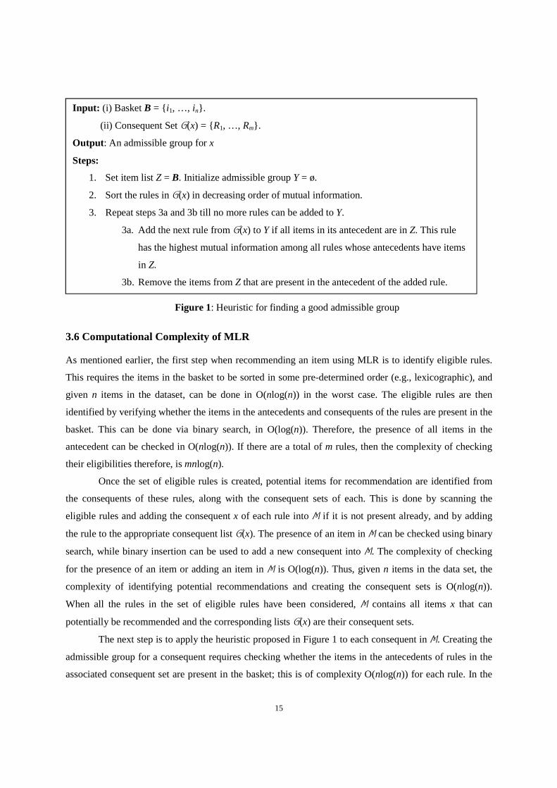
The heuristic to find an admissible group for a consequent x is shown in Figure 1. The intuition is

to keep adding rules with high mutual information into the admissible group without violating

admissibility until no more rules can be added. Hence, the rules are arranged in decreasing order of

mutual information and are added to the admissible group starting from the rule with highest mutual

information until all the items in the basket are covered or all the rules have been considered. By selecting

rules with higher mutual information, the heuristic ensures that the solution does not include two or more

rules from the consequent set that are subsumed by a single rule from that set.

15

Figure 1: Heuristic for finding a good admissible group

3.6 Computational Complexity of MLR

As mentioned earlier, the first step when recommending an item using MLR is to identify eligible rules.

This requires the items in the basket to be sorted in some pre-determined order (e.g., lexicographic), and

given n items in the dataset, can be done in O(nlog(n)) in the worst case. The eligible rules are then

identified by verifying whether the items in the antecedents and consequents of the rules are present in the

basket. This can be done via binary search, in O(log(n)). Therefore, the presence of all items in the

antecedent can be checked in O(nlog(n)). If there are a total of m rules, then the complexity of checking

their eligibilities therefore, is mnlog(n).

Once the set of eligible rules is created, potential items for recommendation are identified from

the consequents of these rules, along with the consequent sets of each. This is done by scanning the

eligible rules and adding the consequent x of each rule into M if it is not present already, and by adding

the rule to the appropriate consequent list G(x). The presence of an item in M can be checked using binary

search, while binary insertion can be used to add a new consequent into M. The complexity of checking

for the presence of an item or adding an item in M is O(log(n)). Thus, given n items in the data set, the

complexity of identifying potential recommendations and creating the consequent sets is O(nlog(n)).

When all the rules in the set of eligible rules have been considered, M contains all items x that can

potentially be recommended and the corresponding lists G(x) are their consequent sets.

The next step is to apply the heuristic proposed in Figure 1 to each consequent in M. Creating the

admissible group for a consequent requires checking whether the items in the antecedents of rules in the

associated consequent set are present in the basket; this is of complexity O(nlog(n)) for each rule. In the

Input: (i) Basket B = { i1, …, in}.

(ii) Consequent Set G(x) = {R1, …, Rm}.

Output : An admissible group for x

Steps:

1. Set item list Z = B. Initialize admissible group Y = ø.

2. Sort the rules in G(x) in decreasing order of mutual information.

3. Repeat steps 3a and 3b till no more rules can be added to Y.

3a. Add the next rule from G(x) to Y if all items in its antecedent are in Z. This rule

has the highest mutual information among all rules whose antecedents have items

in Z.

3b. Remove the items from Z that are present in the antecedent of the added rule.

16

worst case, items in the antecedents of all m rules may have to be checked for their presence in the basket;

this is of complexity O(mnlog(n)). This procedure has to be repeated for every possible consequent, and

therefore the worst case complexity of the heuristic is O(mn2log(n)).

The probabilities can be estimated for each item in M using the rules in the admissible groups in

O(m). Across all items therefore, the complexity is O(mn). The item with highest estimated probability

can be identified in O(n), through a single scan of M.

Thus, the overall complexity of MLR is O(mn2log(n)), which is linear in the number of rules

mined, and has a low-order polynomial complexity in the number of items in the dataset. Since the size of

a typical basket is much smaller than n, the average complexity should be much better.

4. Experiments

We conduct a large number of systematic experiments on two real data sets to investigate the quality of

recommendations made by MLR. First, we conduct experiments comparing recommendations made using

the optimal approach to identify admissible groups (i.e., formulation AG) with those made by the greedy

heuristic presented in Figure 1. Then, we conduct experiments comparing recommendations made using

MLR with various benchmarks including the single rule approaches of Zaïane (2002) and Wang and Shao

(2004), and the rule combination methods of Li et al. (2001) and Lin et al. (2002) (we compare the

performance of MLR with non-rule based approaches in Section 5). All the experiments are performed on

a Pentium Dual Core machine (2.6 GHz) with 4GB of RAM.

4.1 Data

We use two real datasets from the FIMI repository (http://fimi.cs.helsinki.fi/data/) in our experiments.

Retail is a market basket data set collected from a Belgian retail store (Brijs et al. 1999) while BMS-POS

is a point-of-sales dataset collected from a large electronics retailer (Zheng et al. 2001). The basic

characteristics of the two datasets are shown in Table 3.

Characteristics Retail BMS-POS Number of items 16,470 1,657 Number of transactions 88,162 515,597 Average transaction length 10.3 6.5

Table 3: Dataset characteristics

Both datasets have the items in the transactions ordered lexicographically based on their labels.

We randomize the ordering of items in each transaction in order to avoid any bias that might result from

this pre-ordering of the items.

17

4.2 MLR vs Rule-based Systems: Experimental Setup

The experiments involve performing five-fold cross validation tests using these datasets. In the

experiments, baskets are provided to the recommender systems (MLR and the relevant benchmark) and

the number of successful recommendations made by each approach is tracked. The experiments are

designed to mimic the interactions of a customer at a web site to the extent possible. The recommender

system can recommend items every time a customer adds an item to the basket. In order to replicate this

process, each transaction in the test dataset is used to create multiple test baskets iteratively. The first

basket created from a transaction contains the first item in the transaction. Each recommender system

recommends an item for potential addition into the basket. If the recommended item is present in the

remainder of the transaction, the recommendation is considered successful, and the recommended item is

then added to the basket to create the next basket. If both systems recommend different items

successfully, both the items are added to the basket to avoid any potential bias from the addition of just

one of them.4 If neither recommendation is successful, a randomly selected item from the remainder of

the transaction is added to the basket. This process is repeated for the transactions until at least half of the

items in the transactions are included in the basket.5 This is repeated for every transaction in the test

dataset. The approaches are compared based on average accuracy of recommendations.

4.3 Finding the Best Admissible Group: Optimal vs Heuristic Approaches

As part of the MLR process, we need to identify the best admissible group from the many combinations

that might exist. We had shown in Section 3.4 that this problem is NP-Hard, and can be represented as the

set-partitioning problem AG. Later, we proposed a heuristic to achieve the same end (Figure 1). In our

first set of experiments, we compare these two versions of MLR – one using the optimal solution from the

set partitioning problem AG, and the other from the heuristic to understand the practical impact on

recommendation accuracy of using the heuristic. Table 4 shows the results of the experiments.

These results show that while using the optimal admissible groups sometimes does lead to more

successful recommendations, the improvement in performance is very small. For the experiments

conducted on the Retail dataset, the results are virtually identical. The differences are greater for the

experiments conducted on the dataset BMS-POS. However, none of the differences are statistically

significant. We also found that the number of instances when the heuristic and optimal approaches choose

different admissible groups is also very small. At the same time, the time taken by the heuristic for

4 Experiments conducted by randomly adding one of the items to the basket yielded similar results. 5 The results were similar when baskets are created until all items of a transaction but one are included in the basket.

18

making recommendations is about half the time taken by the optimal approach. Incorporating an integer

programming solver into a recommender system is worthwhile only if the benefits over easily

implemented procedures are substantial. Given the results of these experiments, that does not seem to be

the case. Consequently, all the other results reported in this paper are based on using the heuristic. Of

course, in situations where the optimal approach is viable, the results are likely to be better than those

currently being reported.

Dataset Confidence # of baskets # of Successful Recommendations Optimal Heuristic

Retail

30.00% 52,246 13,036 13,036 40.00% 46,720 12,837 12,837

50.00% 44,767 12,793 12,793

60.00% 37,144 10,970 10,969

BMS-POS

30.00% 301,100 97,362 96,902 40.00% 275,274 93,586 93,174 50.00% 231,700 86,571 86,321

60.00% 179,756 76,604 76,542

Table 4: Comparing optimal and heuristic approaches

4.4 MLR vs Single-Rule Based Approaches

Several experiments are conducted to compare MLR with the single rule based approaches of Zaïane

(2002) and Wang and Shao (2004). As the improvements achieved by MLR over both the single-rule

based approaches are very similar, we present only the results comparing MLR with the approach of

Zaïane (2002). In the first set of experiments, the rules are mined from the training datasets using a

support threshold of 0.2%6 and confidence thresholds of 30%, 40%, 50% and 60% (increasing the

confidence threshold beyond 60% generates very few rules).

4.4.1 MLR Uses Multiple Rules

When making recommendations using MLR, the admissible group corresponding to the recommended

item may contain one or multiple rules. When an item is recommended using an admissible group with

only one rule, it is typically the same as that recommended by the single-rule based benchmark. However,

significant improvements in performance are observed when MLR recommends items using admissible

groups with multiple rules. Table 5 presents the results for those instances for which items are

6 This was one of the support thresholds used by Zheng et al. (2001).

19

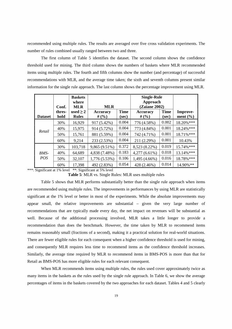
recommended using multiple rules. The results are averaged over five cross validation experiments. The

number of rules combined usually ranged between two and three.

The first column of Table 5 identifies the dataset. The second column shows the confidence

threshold used for mining. The third column shows the numbers of baskets where MLR recommended

items using multiple rules. The fourth and fifth columns show the number (and percentage) of successful

recommendations with MLR, and the average time taken; the sixth and seventh columns present similar

information for the single rule approach. The last column shows the percentage improvement using MLR.

Dataset

Conf. thres-hold

Baskets where MLR

used ≥ 2 Rules

MLR

Single-Rule Approach

(Zaïane 2002) Improve-ment (%)

Accuracy # (%)

Time (sec)

Accuracy # (%)

Time (sec)

Retail

30% 16,929 917 (5.42%) 0.004 776 (4.58%) 0.002 18.20%***

40% 15,975 914 (5.72%) 0.004 773 (4.84%) 0.001 18.24%***

50% 15,761 881 (5.59%) 0.004 742 (4.71%) 0.001 18.71%***

60% 9,214 233 (2.53%) 0.004 211 (2.29%) 0.001 10.43%

BMS-POS

30% 103,718 9,865 (9.51%) 0.372 8,523 (8.22%) 0.019 15.74%***

40% 64,689 4,838 (7.48%) 0.183 4,277 (6.61%) 0.018 13.14%***

50% 32,107 1,776 (5.53%) 0.106 1,495 (4.66%) 0.016 18.78%***

60% 17,398 492 (2.83%) 0.054 428 (2.46%) 0.014 14.90%** ***: Significant at 1% level **: Significant at 5% level

Table 5: MLR vs. Single Rules: MLR uses multiple rules

Table 5 shows that MLR performs substantially better than the single rule approach when items

are recommended using multiple rules. The improvements in performances by using MLR are statistically

significant at the 1% level or better in most of the experiments. While the absolute improvements may

appear small, the relative improvements are substantial – given the very large number of

recommendations that are typically made every day, the net impact on revenues will be substantial as

well. Because of the additional processing involved, MLR takes a little longer to provide a

recommendation than does the benchmark. However, the time taken by MLR to recommend items

remains reasonably small (fractions of a second), making it a practical solution for real-world situations.

There are fewer eligible rules for each consequent when a higher confidence threshold is used for mining,

and consequently MLR requires less time to recommend items as the confidence threshold increases.

Similarly, the average time required by MLR to recommend items in BMS-POS is more than that for

Retail as BMS-POS has more eligible rules for each relevant consequent.

When MLR recommends items using multiple rules, the rules used cover approximately twice as

many items in the baskets as the rules used by the single rule approach. In Table 6, we show the average

percentages of items in the baskets covered by the two approaches for each dataset. Tables 4 and 5 clearly

20

demonstrate that increasing the coverage of items in the baskets substantively improves the performance

of the recommender system. Since all the items in these baskets rarely co-occur simultaneously in

transactions, they do not appear as antecedents of any rule. The rules that exist – which get used by the

benchmark – cover a relatively small percentage of items in the baskets. By combining rules, MLR is

able to improve the coverage and thereby perform better than the benchmark.

Dataset Confidence Threshold

% of Items Covered when MLR Uses Multiple Rules

MLR Single-Rule Approach

Retail

30% 56.26% 26.95%

40% 56.76% 26.83%

50% 56.46% 26.67%

60% 46.84% 23.42%

BMS-POS

30% 85.90% 53.22%

40% 78.01% 48.34%

50% 76.86% 44.84%

60% 83.70% 45.59% Table 6: Fraction of basket covered when MLR uses multiple rules

4.4.2 MLR Uses One Rule

For completeness, we present the results for instances when MLR uses single rules in Table 7. Given that

both approaches recommend the same item often, the results are as expected – the qualities of the

recommendations provided by the approaches are quite similar.

Dataset

Conf. thres-hold

Baskets where MLR used 1 Rule

MLR Single-Rule Approach

(Zaïane 2002)

Improvement (%)

Accuracy # (%)

Time (secs)

Accuracy # (%)

Time (secs)

Retail

30% 35,278 12,058 (34.18%) 0.003 12,054 (34.17%) 0.001 0.04%

40% 30,705 11,862 (38.63%) 0.003 11,856 (38.61%) 0.001 0.05%

50% 28,966 11,852 (40.92%) 0.003 11,845 (40.89%) 0.001 0.06%

60% 27,904 10,693 (38.32%) 0.003 10,690 (38.31%) 0.001 0.03%

BMS-POS

30% 199,542 86,977 (43.59%) 0.093 86,968 (43.58%) 0.012 0.01%

40% 213,461 88,707 (41.56%) 0.076 88,657 (41.53%) 0.013 0.06%

50% 201,471 84,883 (42.13%) 0.057 84,765 (42.07%) 0.012 0.14%

60% 163,312 76,400 (46.78%) 0.040 76,279 (46.71%) 0.012 0.16% Table 7: MLR vs. Single Rules: MLR also uses single rules

Table 8 shows the percentages of items in the baskets covered by the rules used by the two

approaches. It is clear that the percentages of items in these baskets covered by the rules used by the two

21

approaches are very close, and furthermore, the majority of items in the baskets are covered. Hence, the

accuracies of both the approaches are similar.

Dataset Confidence Threshold

% of Items Covered When MLR Uses Single Rules

MLR Single-Rule Benchmark

Retail

30% 60.58% 58.86%

40% 62.51% 60.71%

50% 63.67% 61.88%

60% 56.48% 54.86%

BMS-POS

30% 93.91% 93.08%

40% 88.13% 87.18%

50% 82.52% 81.56%

60% 81.49% 80.76% Table 8: Fraction of basket covered when MLR uses single rules

The performances of both approaches are much better when MLR recommends items using single rules

(the fourth column of Table 7) as compared to when it recommends items using multiple rules (the fourth

column of Table 5). As mentioned earlier, the items in the baskets for which MLR makes

recommendations using multiple rules co-occur less frequently in transactions. However, that is not the

case for the baskets for which MLR recommends items using single rules. As a result, it is far more

difficult to recommend items that are likely to be purchased in the former case than in the latter; this

difficulty is reflected in the marked differences in successful recommendations. When single rules are

used for recommending items for the baskets covered in Table 5, recommendations are significantly

worse than when MLR is used. Also, as expected, MLR requires less time to recommend items when

using single rules (the fifth column of Table 7) than when using multiple rules (the fifth column of Table

5) because the available numbers of eligible rules are fewer in the former case.

4.4.3 Experiments with Different Supports

We perform additional experiments on Retail at support thresholds 0.1% and 0.3% to analyze the

robustness of the two approaches to changes in the support threshold. The results are shown in Table 9.

We present results only for those instances where MLR recommends items using multiple rules, as the

performances of MLR and the benchmark are again quite similar for the other instances.

MLR performs better when items are recommended using multiple rules regardless of the support

and confidence thresholds used for mining. The improvements are statistically significant, with an

exception only when rules mined at 60% confidence thresholds are used. The improvement in

performance is smaller when the rules mined at higher support thresholds are used. For example, the

22

improvement achieved by using MLR is 23.25% when rules mined at support and confidence thresholds

of 0.1% and 30%, respectively, are used, compared to 14.83%, when rules mined at 0.3% support

threshold and 30% confidence threshold are used. One possible reason could be the more frequent use of

rules with higher supports by the single rule approach when rules mined at higher support thresholds are

used. Rules with higher supports are more reliable. Hence, the scope for improvement by using MLR is

smaller.

Sup. thre-shold

Conf. thre-shold

Baskets where MLR

used ≥ 2 Rules

MLR Single-Rule Approach

Improvement (%)

Accuracy # (%)

Time (sec)

Accuracy # (%)

Time (sec)

0.1%

30% 24,616 1141 (4.63%) 0.013 926 (3.76%) 0.004 23.25%***

40% 22,818 1106 (4.85%) 0.012 901 (3.95%) 0.004 22.80%***

50% 22,212 1006 (4.53%) 0.012 818 (3.68%) 0.004 22.99%***

60% 14,380 340 (2.37%) 0.010 298 (2.08%) 0.004 14.08%*

0.3%

30% 12,494 780 (6.25%) 0.002 680 (5.44%) 0.001 14.83%***

40% 12,020 780 (6.49%) 0.002 679 (5.65%) 0.001 14.87%***

50% 11,884 761 (6.40%) 0.002 661 (5.56%) 0.001 15.16%*

60% 6,467 171 (2.64%) 0.002 159 (2.46%) 0.001 7.28% ***: significant at 1% level or better, *: significant at 10% level

Table 9: Multiple support levels on Retail: MLR uses multiple rules

4.4.3 Recommending Multiple Items

We also perform experiments in which two items are recommended for each basket by both approaches.

BMS-POS is used for the experiments and the rules are mined at a support threshold of 0.2% and

confidence thresholds of 15%, 20%, 25%, 30% and 35%. The reason for using rules mined at these

thresholds is that the average number of items that can be recommended per basket is four or more when

rules mined at these thresholds are used.7 Table 10 shows the results of the experiments on BMS-POS for

those baskets for which MLR recommends both items using multiple rules; the performance improvement

is observed to be significant. The differences in the performances of the two approaches are not

significant when either one or both items are recommended by MLR using single rules.

7 The Retail dataset was not used because we cannot obtain more than two recommendations on average per basket for any reasonable confidence level when using rules mined at a support threshold of 0.2%.

23

Confidence # of

baskets

MLR Accuracy

#(%)

Single Rule Accuracy

#(%)

Improvement (%)

15% 43,360 4,407 (10.16%) 3,569 (8.23%) 23.49%***

20% 41,916 3,851 (9.19%) 3,236 (7.72%) 18.99%***

25% 38,338 3,137 (8.18%) 2,745 (7.16%) 14.26%***

30% 30,474 2,086 (6.84%) 1,891 (6.20%) 10.31%***

35% 19,886 1,080 (5.43%) 1,002 (5.04%) 7.70% ***: significant at 1% level or better

Table 10: MLR vs. Single Rule when 2 items are recommended (BMS-POS)

4.5 MLR vs Rule-Combination Approaches

Various experiments were conducted comparing MLR with the rule combination approach of Lin et al.

(2002) and the CMAR approach of Li et al. (2001). The improvement from using MLR compared to the

approach of Lin et al. (2002) was more than the improvement over CMAR. Therefore, we only report

results comparing MLR with CMAR.

CMAR was developed for classification, and therefore we had to adapt it to work in a product

recommendation context. In a transactional data set, the consequents of eligible rules are analogous to

classes to which a customer may belong. CMAR works as follows. When a basket is provided to CMAR,

it evaluates the sums of the weighted chi-squares of the rules in the individual consequent sets, and the

item corresponding to the consequent set with the highest sum is recommended. The chi-square of a rule

indicates the correlation between the items in the rule. Rules in a consequent set with highest sum of

weighted chi-square have highest correlation with each other and the consequent corresponding to that

consequent set is expected to have the highest probability of being selected by the customer (Li et al.

2001). The sum of the weighted chi-squares of the rules in a consequent is ∑ iUiU?j iU, where k. is the chi-

square statistic of a rule with antecedent P and consequent c, and maxc2 is evaluated as:

lg�k. = \minXsup�� , sups�Y − sup�� sups�|t| ]

.|T|v

where v = �Lwx�yz{|� + �

yz{�|}|#yz{|�� + �|}|#yz{�� yz{|� + �

|~|#yz{��|}|#yz{|��, sup(P) = number of transactions with items in P,

sup(c) = number of transactions with consequent c, and

|T| = total number of transactions.

Readers are referred to Li et al. (2001) for additional details of their approach.

As with the previous comparison, experiments are first performed using rules mined at a support

threshold of 0.2% and confidence thresholds of 30%, 40%, 50% and 60% on both the Retail and BMS-

24

POS datasets. Table 11 shows the results of the experiments over all the baskets.8 It is evident that the

improvements in the performances achieved by using MLR are statistically significant except when rules

mined at 60% confidence threshold are used.

Confidence threshold

# of Baskets MLR Accuracy #(%) CMAR Accuracy

#(%) Improvement

(%)

Retail

30% 51,417 12,058 (23.45%) 11,635 (22.63%) 3.64%***

40% 45,909 11,840 (25.79%) 11,515 (25.08%) 2.82%**

50% 43,974 11,804 (26.84%) 11,498 (26.15%) 2.66%**

60% 36,751 10,506 (28.59%) 10,439 (28.40%) 0.65%

BMS-POS

30% 59,111 17,727 (29.99%) 15,617 (26.42%) 13.51%*** 40% 54,366 17,317 (31.85%) 16,958 (31.19%) 2.12%** 50% 45,671 16,153 (35.37%) 15,753 (34.49%) 2.54%*** 60% 35,352 14,547 (41.15%) 14,347 (40.58% 1.40%

***: significant at 1% level or better **: significant at 5% level

Table 11: MLR vs. CMAR

We conducted additional experiments on the Retail dataset using rules mined at support

thresholds of 0.1% and 0.3%. The relative performances of the two approaches are very similar for those

experiments as well, and are not reported here for brevity.

5. Comparisons with Collaborative Filtering and Matrix Factorization

While rule based recommender systems are commonly used in the retail domain (e.g., Forsblom et al.

2009), and they form integral components of many commercial software (IBM 2009a, 2009b, 2010), no

individual system is known to be universally better than others. In this section, we provide evidence of the

broad applicability of MLR by comparing it to two state-of-the-art techniques – collaborative filtering and

matrix factorization. Both approaches are widely used for providing recommendations and have been

shown to perform well (Linden 2003, Deshpande and Karypis 2004, Koren et al. 2009; Ekstrand et al.

2011). We present results from several experiments conducted on the Retail and BMS-POS data sets,

comparing the quality of recommendations from MLR with those generated using these approaches.

While two approaches to collaborative filtering are popular, Jannach et al. (2011) point out that

the need to handle millions of users in large e-commerce systems makes user-based collaborative filtering

impractical in real time environments. Item-based collaborative filtering on the other hand makes

predictions based on the similarity between items. These can be computed offline, which makes item-

8 We provide results aggregated over all the baskets here because, unlike in previous experiments, both MLR and CMAR use multiple rules whenever possible.

25

based collaborative filtering a viable approach for making real-time recommendations. Also, item-based

collaborative filtering is designed to generate recommendations using transactional data (Linden et al.

2003). Therefore, we use item-to-item collaborative filtering in our experiments.

The Netflix Prize competition revealed that matrix factorization methods can also be very

effective in making recommendations. These methods represent users and items via latent factors

identified from the data, with an item being recommended to a user when the item and user are similar

vis-à-vis these factors (Koren et al. 2009). A well-known matrix factorization technique for recommender

systems is singular value decomposition (SVD), and one version of which, called FunkSVD, has been

popularized by Simon Funk (2006). We use FunkSVD (Funk 2006) in our experiments.

We use the collaborative filtering and FunkSVD implementations provided by Ekstrand et al.

(2011) in an open source project named Lenskit (lenskit.grouplens.org). As noted by the authors, Lenskit

provides carefully tuned implementations of these leading algorithms. We note that in their experiments

on three separate datasets, Ekstrand et al. (2011) find FunkSVD to perform the best on two datasets and

the item-to-item collaborative filtering approach to perform the best on the third.

We provide brief descriptions of the two methods below; specific details about the

implementations can be found in Ekstrand et al. (2011).9 The idea behind the item-based approach is to

find items that are rated as similar to the items that have been liked by a target user. Given a dataset

involving m items, the item-based collaborative filtering procedure implemented by Ekstrand et al.

requires two parameters as inputs – a model size (k) and a neighborhood size (l). The system computes

scores for the items being considered for recommendation by multiplying an mµm similarity matrix

(model) with a column vector representing the current basket of the user (the vector has a 1 for all items

present in the basket and a 0 for the other items). The model size is the number of similarities retained in

each column of the model; other similarities are set to 0. The neighborhood size is the number of

similarities used to calculate the score of an item; other similarities are ignored. The item with the highest

score is recommended.

The matrix factorization technique determines latent factors, associates each user with a user-

factor vector and each item with an item-factor vector, and makes predictions using the inner product of

such vectors. The parameters of the model are learned with the objective of minimizing the differences

between predicted and actual ratings while avoiding over-fitting (Koren et al. 2009). FunkSVD

accomplishes this using a stochastic gradient descent learning algorithm.

9 Interested readers are directed to Deshpande and Karypis (2004) for additional details on collaborative filtering, and to Funk (2006) and Koren et al. (2009) for details on FunkSVD.

26

We perform, as before, five-fold cross validation experiments on both the Retail and BMS-POS

datasets. We use a support threshold of 0.2% and confidence thresholds of 30%, 40%, 50% and 60% for

MLR. We experimented with various values of model sizes (up to 500) and neighborhood sizes (up to

150) for collaborative filtering.

While FunkSVD was originally designed for ratings of user-item pairs (like any matrix

factorization technique), it has been observed to work well for binary data if all the zero values are

replaced with a small number like 0.1 (XLVector 2012). Therefore, we modify the Retail and BMS-POS

datasets in this manner to run FunkSVD. The resulting datasets are dense and cannot be used in their

entirety by Lenskit. Therefore, for each original training dataset from Retail, we randomly select 2,000

transactions for model building. We are able to use 10,000 transactions (again randomly selected) as the

training datasets for BMS-POS, because this dataset has much fewer items than Retail. All the modified

datasets have more than ten million values for user-item pairs (the largest dataset used by Ekstrand et al.

has ten million values). We experimented with other (smaller) numbers of randomly selected transactions

for creating ratings datasets – the results do not differ significantly.

Dataset Confidence Threshold

Accuracy (%) Improvement

over CF (%)

Improvement over FunkSVD

(%) CF FunkSVD MLR

Retail

30% 32.90% 43.91% 47.27% 43.65%*** 7.64%***

40% 33.85% 45.01% 48.41% 43.00%*** 7.55%***

50% 34.42% 45.44% 48.87% 41.98%*** 7.55%***

60% 36.10% 47.64% 52.12% 44.40%*** 9.41%***

BMS-POS

30% 45.21% 47.30% 50.07% 10.76%*** 5.86%***

40% 48.16% 50.43% 53.48% 11.04%*** 6.05%***

50% 50.21% 52.74% 55.71% 10.96%*** 5.64%***

60% 52.18% 55.24% 57.93% 11.02%*** 4.86%***

***: significant at 1% level or better Table 12: MLR vs. Collaborative filtering (CF) and FunkSVD

We provide the results of the experiments in Table 12. Baskets are created from each transaction

in the test datasets by randomly selecting half the items in the transaction – the baskets are identical for all

the approaches. The results presented are for those transactions for which all the approaches generate

recommendations and are averaged over all cross-validation experiments. The performance of the

collaborative filtering system is not very sensitive to changes in the model and neighborhood sizes. We

report the results for the experiments with model size 500 and neighborhood size 150 since the system’s

27

performance is a little better with these settings. For FunkSVD, we use the default settings of the

implementation – other settings provided similar or inferior performances.

Table 12 presents the quality of recommendations provided by each approach for each dataset and

confidence threshold. The relative improvements achieved by MLR over the other approaches are

statistically significant for every experiment on each of the datasets. These results show that MLR is not

only superior to other rule-based approaches for the datasets we have examined, but outperforms other

state-of-the-art approaches as well.

6. Conclusions and Managerial Implications

Traditional approaches that use only a single rule for recommending items typically ignore items in the

baskets of the customer that may be present in the antecedents of other rules. We propose an approach –

Maximum Likelihood Recommendations (MLR) – to combine multiple rules to recommend items in order

to cover as many items of the basket as possible. While a few methods have been proposed to combine

rules, these are all ad hoc, without a robust theoretical basis. In contrast, MLR has a strong theoretical

foundation – it recommends items using rules that maximize the likelihood of generating the true

underlying distribution of the dataset used for generating the rules. This process identifies the best set of

rules to combine when estimating the probability that a customer will add a recommended item to her

basket.

It is not practical to solve the problem of maximizing likelihood directly however, as it requires

the estimation of parameters from the dataset during run-time. We show that maximizing the likelihood is

equivalent to maximizing the sum of the mutual information values of the participating rules – this result

makes the real-time use of this approach feasible.

We conduct extensive experiments to test the viability of the proposed approach. Comparisons

are made with traditional single-rule based approaches, two methods that have been proposed to combine

rules, and two other state-of-the-art recommendation approaches – collaborative filtering and matrix

factorization. The experiments show that MLR consistently outperforms all the other approaches,

particularly when rules are available for combination. We also find that the performance improvements

are robust across datasets at various support and confidence thresholds.

While the absolute improvements may seem small at first glance, it is important to remember that

recommendations are made on a continuous basis. For instance, during the holiday season in 2012,

Amazon.com sold 306 items per second (Clark, 2012). The 2012 annual report for Amazon.com mentions

that their net sales for the fourth quarter of 2012 amounted to $21.27 billion. If 35% of these revenues are

generated from recommendations (Hosanagar et al. 2012), then even a 1% increase in success rate would

28

amount to an increase in revenues of approximately $70 million every quarter. Such improvements can

lead to increasing revenues by millions of dollars every year for smaller firms as well.

Several characteristics of MLR make it suitable for firms that provide personalized

recommendations to their online customers. The use of probability calculus provides semantic clarity in

an environment that is naturally fraught with uncertainty – at the same time, the approach is able to

deliver recommendations effectively. The robust theoretical basis of MLR makes it very versatile.

Because it compares alternative items to recommend based on their probabilities of purchase, it can be

easily adapted to make recommendations based on expected payoffs associated with the items. This is not

possible with any of the existing approaches, i.e., rule combination, collaborative filtering, or matrix

factorization. The use of probability theory also allows MLR to be easily adapted to use lift-based

approaches to make recommendations if needed – again this is not possible with any of the other

approaches. While we use association rules mined from historical data in our experiments, the approach

can easily accommodate rules provided by human experts. Such rules may be available from marketing

experts for new items that are being offered and for which transactional data are not yet available. MLR

can also use association rules with negations if such rules are found to improve the quality of

recommendations. MLR is computationally quite efficient, taking only a fraction of a second per

recommendation on average – further, this is accomplished using a simple desktop computing

environment. As a result, using MLR instead of the single-rule based approach should not affect the

quality of service during regular operation in commercial environments.

While the results of our experiments with MLR are very encouraging, we note that the

performances of different approaches can be sensitive to the application domain and data characteristics.

For example, our results are consistent with those of Mobasher et al. (2001) with regard to collaborative

filtering – they also found an association rule based approach to outperform a collaborative filtering based

one. However, Sarwar et al. (2000) found evidence to the contrary. Similarly, FunkSVD is shown to

perform better than item-based collaborative filtering on two MovieLens datasets but worse on a Yahoo!

Music dataset (Ekstrand et al. 2011). Given the differences in performances of alternative approaches for

different application domains, firms would be prudent to evaluate the different types of available

approaches in order to identify the best one for their specific context.

Our work opens up several avenues for future research. MLR can serve as a valuable new method

to consider for ensemble-based approaches as its theoretical basis is quite different (and therefore

independent) from those of memory-based approaches such as collaborative filtering and matrix

factorization. It would be useful to develop ways to combine MLR with other extant approaches to

determine which techniques best complement each other. Another interesting opportunity is to examine

how MLR could be extended to incorporate probabilistic context-based approaches that account for item

29

metadata, user demographics, etc. An important issue that has emerged in recent years is the extent to

which a recommendation technique is vulnerable to manipulations that are often referred to as shilling

attacks (Mobasher et al. 2007). It will be useful to examine in future research how robust MLR is to such

attacks, as compared to extant techniques. Finally, it would be useful to extend recommendation query

languages like REQUEST (Adomavicius et al. 2010) by incorporating a probability-based query interface

that will allow end users to generate recommendations in a flexible and user-friendly manner.

Acknowledgements

The authors would like to thank Michael Ekstrand for his considerable help in using Lenskit for the

experiments that involved collaborative filtering and matrix factorization techniques.

References

1. G. Adomavicius, A. Tuzhilin, and R. Zheng. "REQUEST: A Query Language for Customizing Recommendations." Information Systems Research, vol. 22, no. 1, March 2011.

2. Agrawal, R., Imielinski, T., and Swami, A., 1993. “Mining Association Rules between Sets of Items in Large Databases,” Proc. of the ACM SIGMOD Conference on Management of Data, Washington, D.C., pp. 207-216.

3. Balas, E. and Padberg, M, 1976. “Set Partitioning: A Survey,” SIAM Review (18), pp. 710–760.

4. Bayardo, R. J. Jr. , Agrawal, R., 1999. “Mining the Most Interesting Rules,” Proceedings of the fifth ACM SIGKDD International Conference on Knowledge Discovery and Data Mining, pp.145-154, August 15-18, San Diego, California, United States.

5. Berry, M. and Linoff , G., 2004. “Data Mining and Techniques,” 2nd Ed. Wiley Computer Publishing, New York.

6. Brijs, T., “Retail Market Basket Data Set,” http://fimi.cs.helsinki.fi/data/

7. Clark, K. 2012. “Amazon Has Best Holiday Season Ever, Selling 306 Items Per Second”, Forbes.com, December 27, 2012. http://www.forbes.com/sites/kellyclay/2012/12/27/amazon-has-best-holiday-season-ever-selling-306-items-per-second/

8. Deshpande, M. and Karypis, G. 2004. “Item-based Top N Recommendation Algorithms,” ACM Transactions on Information Systems, 22(4), pp. 143-177.

9. Domingos, P. and Pazzani, M., 1997. “On the Optimality of the Simple Bayesian Classifier under Zero-One Loss,” Machine Learning (29), pp. 103-130.

10. Ekstrand, M.D., Ludwig, M., Konstan, J.A. and Riedl, J.T. 2011. “Rethinking the Recommender Research Ecosystem: Reproducibility, Openness, and LensKit,” Proceedings of the fifth ACM conference on Recommender systems, 2011.

30

11. Ergun O., Kuyzu, G. and Savelsbergh, M., 2007. “Reducing Truckload Transportation Costs Through Collaboration,” Transportation Science, 41 (2), May 2007, pp. 206-221.

12. Forsblom, A., Nurmi, P., Floreen, P., Peltonen, P. and Saarikko, P. 2009. “Massive- An Intelligent Shopping Assistant,” Proceedings of the Workshop on Personalization in Mobile and Pervasive Computing, Trento, Italy, 2009.

13. Funk, S. 2006. “Netflix Update: Try This at Home,” http://sifter.org/~simon/journal/20061211.html. Last accessed on June 20, 2012.

14. Gordon, L. 2008. “Leading Practices in Market Basket Analysis. How Top Retailers are Using Market Basket Analysis to Win Margin and Market Share,” Factpoint Group. 2008.

15. Hanson, W., 2000. “Principles of Internet Marketing,” South-Western College Publishing, Cincinnati, Ohio.

16. Hastie, T., Tibshirani, R.and Friedman, J., 2009. “The Elements of Statistical Learning,” Data Mining, Inference and Prediction, 2nd Ed. Springer, New York.

17. Häubl, G. and Trifts, V., 2000. “Consumer Decision Making in Online Shopping Environments: The Effects of Interactive Decision Aids,” Marketing Science (19:1), pp. 4-21.

18. Hosanagar, K., Fleder, D.M., Lee, D., and Buja, A., 2012. “Will the Global Village Fracture Into Tribes: Recommender Systems and their Effects on Consumers,” NET Institute Working Paper No. 08-44.

19. IBM. 2009a. “IBM SPSS Retail Market Basket Analysis,” ftp://service.boulder.ibm.com/ software/uk/ data/ibm-spss-retail-datasheet.pdf. Accessed on April 11, 2012.

20. IBM. 2009b. “Retail Market Basket Analysis,” https://www-304.ibm.com/easyaccess/fileserve/ ?contentid=193973. Accessed on April 11, 2012.

21. IBM. 2010. “Predictive analytics for retail market basket analysis”, ftp://public.dhe.ibm.com/ common/ssi/ecm/en/yts03013gben/YTS03013GBEN.PDF. Accessed on April 11, 2012.

22. Jannach, D., Zanker, M., Felfernig, A. and Friedrich, G. 2011. “Recommender Systems: An Introduction,” Cambridge University Press, pp. 31-35, 2011.

23. Koren, Y., Bell, R. and Volinsky, C. 2009. "Matrix Factorization Techniques for Recommender Systems", IEEE Computer (42:8), pp. 30-37, August, 2009.

24. Kullback, S., 1959. “Information Theory and Statistics,” Wiley, New York.

25. Lewin, B.A. 2009. “Beyond The Grocery and Retail Store: Applying Market Basket Analysis to the Service Industry,” A 1010Data White Paper. 2009.

26. Li, W., Han, J., Pei, J., 2001. “CMAR: Accurate and Efficient Classification Based on Multiple Class-Association Rules,” Proceedings IEEE International Conference on Data Mining, 2001.

31

27. Lin, W., Alvarez, S. A. and Ruiz, C. 2002. Efficient Adaptive-Support Association Rule Mining for Recommender Systems. Data Mining and Knowledge Discovery, Vol. 6, Issue 1, January 2002, pp. 83-105.

28. Linden, G., Smith, B. and York, J. 2003. “Amazon.com Recommendations Item-to-Item Collaborative Filtering,” IEEE Internet Computing (7:1), January-February 2003.

29. Liu, B., Ma, Y., Wong, C.K., 2003. “Scoring the Data Using Association Rules,” Applied Intelligence, 2003, 18, pp. 119–135.

30. Mobasher, B., Dai, H., Luo, T. and Nakagawa, M. 2001. “Effective Personalization Based on Association Rule Discovery from Web Usage Data,” Proceedings of the 3rd International Workshop on Web Information and Data Management, WIDM 2001.

31. Mobasher, B., Burke, R., Bhaumik, R.,Williams, C.: Towards trustworthy recommender systems: an analysis of attack models and algorithm robustness. ACM Transactions on Internet Technology. 7(4) Article 23 (2007).

32. Ng, R. T., Lakshmanan, L., V., S., Han, J. and Pang, A. 1998. Exploratory Mining and Pruning Optimizations of Constrained Associations Rules, Proceedings of the 1998 ACM SIGMOD International Conference on Management of Data, p.13-24, June 01-04, 1998, Seattle, Washington, United States.

33. Pathak, B., Garfinkel, R., Gopal, R., Venkatesan, R. and Yin, F. 2010. Empirical Analysis of the Impact of Recommender Systems on Sales, Journal of Management Information Systems, (27:2), Fall 2010, pp. 159-188.

34. Sarwar, B., Karypis, G., Konstan, J., and Riedl. ,J., 2000. “Analysis of Recommendation Algorithms for E-Commerce,” EC’00, Minneapolis, Minnesota.

35. Tam, K. Y. and Ho, S. Y., 2003. “Web Personalization: Is it Effective?,” IT Professional, 5,5, pp. 53-57.

36. Wang, F.H. and Shao, H.M., 2004. “Effective Personalized Recommendation Based on Time-Framed Navigation Clustering and Association Mining,” Expert Systems with Applications, (27), pp. 365–377

37. Wickramaratna, K., Kubat, M. and Premaratne, K., 2009. “Predicting Missing Items in Shopping Carts,” IEEE Transactions on Knowledge and Data Engineering, 21, pp. 985-998.

38. XLVector. 2012. XLVector – Recommender System. http://xlvector.net/blog/?p=465. Last accessed on July 7 2012.

39. Zaïane, O.R., 2002. “Building a Recommender Agent for e-Learning Systems,” Proceedings of the International Conference on Computers in Education.

40. Zaki, M. J., 2000. “Generating Non-Redundant Association Rules,” KDD '00: Proceedings of the sixth ACM SIGKDD International Conference on Knowledge Discovery and Data Mining.

41. Zheng, Z., Kohavi, R., Mason, L., 2001. “Real World Performance of Association Rule Algorithms,” Proc. 7th ACM SIGKDD International Conference on Knowledge Discovery and Data Mining. ACM Press, New York, pp. 401–406.