1

A Comparative Study of Recommendation Algorithms in E-

Commerce Applications

Zan Huang Department of Supply Chain and Information Systems

Smeal College of Business Pennsylvania State University

zanhuang@psu.edu

Daniel Zeng and Hsinchun Chen Department of Management Information Systems

Eller College of Management University of Arizona

{zeng, hchen}@eller.arizona.edu

Abstract

We evaluate a wide range of recommendation algorithms on e-commerce-related datasets.

These algorithms include the popular user-based and item-based correlation/similarity

algorithms as well as methods designed to work with sparse transactional data. Data

sparsity poses a significant challenge to recommendation approaches when applied in e-

commerce applications. We experimented with approaches such as dimensionality

reduction, generative models, and spreading activation, which are designed to meet this

challenge. In addition, we report a new recommendation algorithm based on link

analysis. Initial experimental results indicate that the link analysis-based algorithm

achieves the best overall performance across several e-commerce datasets.

Keywords Recommender systems, collaborative filtering, algorithm design and evaluation, e-

commerce

2

1. Introduction Recommender systems are being widely used in many application settings to suggest

products, services, and information items to potential consumers. For example, a wide

range of companies such as Amazon.com, Netflix.com, Half.com, CDNOW, J.C. Penney,

and Procter & Gamble have successfully deployed commercial recommender systems

and reported increased Web and catalog sales and improved customer loyalty. Many

software companies provide stand-alone generic recommendation technologies. The top

five providers include Net Perceptions, Epiphany, Art Technology Group, BroadVision,

and Blue Martini Software. These five companies combined have a total market capital of

over $600 million as of December 2004 (finance.yahoo.com).

At the heart of recommendation technologies are the algorithms for making

recommendations based on various types of input data. In e-commerce, most

recommendation algorithms take as input the following three types of data: product

attributes, consumer attributes, and previous interactions between consumers and

products (e.g., buying, rating, and catalog browsing).

Models based on the product or consumer attributes attempt to explain consumer-

product interactions based on these intrinsic attributes. Intuitively these models learn

either explicitly or implicitly rules such as “Joe likes science fiction books” and “well-

educated consumers like Harry Potter.” Techniques such as regression and classification

algorithms have been used to derive such models. The performances of these approaches,

however, rely heavily on high-quality consumer and product attributes that are often

difficult or expensive to obtain.

Collaborative filtering-based recommendation takes a different approach by utilizing

only the consumer-product interaction data and ignoring the consumer and product

attributes [9]. Based solely on interaction data, consumers and products are characterized

implicitly by their previous interactions. The simplest example of recommendation based

only on interaction data is to recommend the most popular products to all consumers.

Collaborative filtering has been reported to be the most widely adopted and successful

recommendation approach and researchers are actively advancing collaborative filtering

technologies in various aspects including algorithmic design, human-computer

interaction design, consumer incentive analysis, and privacy protection (e.g., [1, 10]).

3

Despite significant progress made in collaborative filtering research, there are several

problems limiting its applications in e-commerce. One major problem is that most

research has focused on recommendation from multi-graded rating data that explicitly

indicate consumers’ preferences, whereas the available data about consumer-product

interactions in e-commerce applications are typically binary transactional data (e.g.,

whether a purchase was made or not). Although algorithms developed for multi-graded

rating data can be applied, typically with some modest modifications, to binary data,

these algorithms are not able to exploit the special characteristics of binary transactional

data to achieve more effective recommendation. A second problem is lack of

understanding of relative strengths and weaknesses of different types of algorithms in e-

commerce applications. The need for such comparative studies is evident in many recent

studies that have proposed new algorithms but only conducted limited comparative

evaluation. The third problem with collaborative filtering as a general-purpose e-

commerce recommendation approach is the sparsity problem, which refers to the lack of

prior transactional and feedback data that makes it difficult and unreliable to infer

consumer similarity and other patterns for prediction purposes. Research on high-

performance algorithms under sparse data is emerging [5, 6, 8, 11], but substantial

additional research effort is needed to provide solid understanding of them.

Our research is focused on addressing the above problems. Our ultimate goal is to

develop a meta-level guideline that “recommends” an appropriate recommendation

algorithm for a given application that demonstrates certain data characteristics. In this

article, we present the initial results of an experimental study towards this goal with two

specific objectives: (a) evaluating collaborative filtering algorithms with different e-

commerce datasets, and (b) assessing the effectiveness of different algorithms with sparse

data.

2. Recommendation Algorithms We now present six types of representative collaborative filtering algorithms including

three algorithms previously designed to alleviate the sparsity problem and a new

algorithm we recently developed based on the ideas from link analysis.

4

We first introduce a common notation for describing a collaborative filtering problem.

The input of the problem is an M × N interaction matrix A = (aij) associated with M

consumers C = {c1, c2,…, cM} and N products P = {p1, p2, …, pN}. We focus on

recommendation that is based on transactional data. That is, aij can take the value of

either 0 or 1 with 1 representing an observed transaction between ci and pj (for example,

ci has purchased pj) and 0 absence of transaction. We consider the output of a

collaborative filtering algorithm to be potential scores of products for individual

consumers that represent possibilities of future transactions. A ranked list of K products

with the highest potential scores for a target consumer serves as the recommendations.

2.1 User-based Algorithm

The user-based algorithm, which has been well-studied in the literature, predicts a target

consumer’s future transactions by aggregating the observed transactions of similar

consumers. The algorithm first computes a consumer similarity matrix WC = (wcst), s, t =

1, 2, …, M. The similarity score wcst is calculated based on the row vectors of A using a

vector similarity function (such as in [1]). A high similarity score wcst indicates that

consumers s and t may have similar preferences since they have previously purchased a

large set of common products. WC·A gives potential scores of the products for each

consumer. The element at the cth row and pth column of the resulting matrix aggregates

the scores of the similarities between consumer c and other consumers who have

purchased product p previously. In other words, the more similar to the target consumer

are the set of consumers who bought the target product, the more likely the target

consumer will also be interested in that product.

2.2 Item-based Algorithm

The item-based algorithm is different from the user-based algorithm only in that product

similarities are computed instead of consumer similarities. This algorithm first computes

a product similarity matrix WP = (wpst), s, t = 1, 2, …, N. Here, the similarity score wpst

is calculated based on column vectors of A. A high similarity score wpst indicates that

products s and t are similar in the sense that they have been co-purchased by many

consumers. A·WP gives the potential scores of the products for each consumer. Here, the

5

element at the cth row and pth column of the resulting matrix aggregates the scores of the

similarities between product p and other products previously purchased by consumer c.

The intuition behind this algorithm is similar: the more similar to the target product are

the products purchased by the target consumer, the more likely he/she will also be

interested in that product. This algorithm has been shown to provide higher efficiency

and comparable or better recommendation quality than the user-based algorithm for many

datasets [3].

2.3 Dimensionality Reduction Algorithm

The dimensionality reduction-based algorithm first condenses the original interaction

matrix and generates recommendations based on the condensed and less sparse matrix to

alleviate the sparsity problem [11]. The standard singular vector decomposition

procedure is applied to decompose the interaction matrix A into 'VZU ⋅⋅ , where U and V

are two orthogonal matrices of size RM × and RN × respectively and R is the rank of

matrix A. Z is a diagonal matrix of size RR× having all singular values of matrix A as its

diagonal entries. The matrix Z is then reduced by retaining only k largest singular values

to obtain Zk. U and V are reduced accordingly to obtain Uk and Vk. As a result,

'kkk VZU ⋅⋅ provides the best lower rank approximation of the original interaction matrix

A that preserves the primary data patterns exist in the data after the “noises” are removed.

Consumer similarities can then be derived from the compact representation based on kU

and 2/1kZ . Recommendations are then generated in the same fashion as described in the

user-based algorithm.

2.4 Generative Model Algorithm

Under this approach, latent class variables are introduced to explain the patterns of

interactions between consumers and products [5, 12]. Typically one can use one latent

class variable to represent the unknown cause that governs the interactions between

consumers and products. The interaction matrix A is considered to be generated from the

following probabilistic process: (1) select a consumer with probability P(c); (2) choose a

latent class with probability P(z|c); and (3) generate an interaction between consumer c

6

and product p (i.e., setting acp to be 1) with probability P(p|z). Thus the probability of

observing an interaction between c and p is given by ∑= zzpPczPcPpcP )|()|()(),( .

Based on the interaction matrix A as the observed data, the relevant probabilities and

conditional probabilities are estimated using a maximum likelihood procedure called

Expectation Maximization (EM). Based on the estimated probabilities, P(c, p) gives the

potential score of product p for consumer c.

2.5 Spreading Activation Algorithm

In our previous research, we have proposed a graph-based recommendation approach

based on the ideas of associative information retrieval [6]. This approach addresses the

sparsity problem by exploring transitive associations between consumers and products in

a bipartite consumer-product graph that corresponds with the interaction matrix A. The

spreading activation algorithms developed in associative information retrieval can then be

adopted to accomplish transitive association exploration efficiently. In this study we used

an algorithm with competitive performance in recommendation applications, the Hopfield

net algorithm [6]. In this approach, consumers and products are represented as nodes in a

graph, each with an activation level μj, j = 1, …, N. To generate recommendations for

consumer c, the corresponding node is set to have activation level 1 (μc = 1). Activation

levels of all other nodes are set at 0. After initialization the algorithm repeatedly performs

the following activation procedure: μj(t + 1) = ( )⎥⎦

⎤⎢⎣

⎡∑−

=

1

0

n

iiijs ttf μ , where fs is the continuous

SIGMOID transformation function or other normalization functions; tij equals η if i and j

correspond to an observed transaction and 0 otherwise (0 < η < 1). The algorithm stops

when activation levels of all nodes converge. The final activation levels μj of the product

nodes give the potential scores of all products for consumer c. In essence this algorithm

achieves efficient exploration of the connectedness of a consumer-product pair within the

consumer-product graph context. The connectedness concept corresponds to the number

of paths between the pair and their lengths and serves as the predictor of occurrence of

future interaction.

7

2. 6 Link Analysis Algorithm

The last algorithm is a new recommendation algorithm which we recently developed

based on the ideas from link analysis research. Link analysis algorithms have found

significant application in Web page ranking and social network analysis (notably, HITS

[7] and PageRank [2]). Our algorithm is an adaptation of the HITS algorithm in the

recommendation context.

The original HITS algorithm distinguishes between two types of Web pages that

pertain to a certain topic: authoritative pages, which contain definitive high-quality

information, and hub pages, which are comprehensive lists of links to authoritative pages.

A given webpage i in the Web graph has two distinct measures of merit, its authority

score ai and its hub score hi. The quantitative definitions of the two scores are recursive.

The authority score of a page is proportional to the sum of hub scores of pages linking to

it, and conversely, its hub score is proportional to the authority scores of the pages to

which it links. These definitions translate to a set of linear equations: jj jii hGa ∑=

and jj iji aGh ∑= , where G is the matrix representing the links in the Web graph. Using

the vector notation, a = (a1, a2, …, an) and h = (h1, h2, …, hn), we can express the

equations in compact matrix form: a = G' · h = G' · G · a and h = G · a = G · G' · h. The

solutions of the above equations correspond to eigenvectors of G' · G (for a) and G · G'

(for h). Computationally, it is often more efficient to start with arbitrary values of a and h

and repeatedly apply a = G' · h and h = G · a with a certain normalization procedure at

each iteration. Subject to some mild assumptions, this iterative procedure is guaranteed to

converge to the solutions [7].

In our recommendation application, consumer-product relationship forms a bipartite

graph consisting of two types of nodes, consumer and product nodes.

A link between a consumer node c and a product node p indicate that p has the potential

to represent part of c’s interest and at the same time c could partially represent product p's

consumer base. Compared to Web page ranking, recommendation requires the

identification of products of interest for individual consumers rather than generally

popular products. As such, we adapt the original authority and hub scores definitions as

follows. We define a product representativeness score pr(p, c0) of product p with respect

8

to consumer c0, which can be viewed as a measure of the "authority" of product p in

terms of the level of interest it will have for consumer c0. Similarly, we define a

consumer representativeness score cr(c, c0) of c with respect to consumer c0, which

measures how well consumer c, as a "hub" for c0, associates with products of interest to

c0.

In contrast to the vector representation of Web page authority and hub scores, we

denote by PR = (prik) the N × M product representativeness matrix where prik = pr(i, k),

and by CR = (crit) the M × M consumer representativeness matrix where crit = cr(i, t).

Directly following the idea of the recursive definition of authority and hub scores, one

would define the product and consumer representativeness scores as PR = A' · CR and CR

= A · PR. Intuitively, the sum of the product representativeness scores of the products

linked to a consumer gives the consumer representativeness score and vice versa.

These obvious extensions of the score definitions have several inherent problems.

First, if a consumer has links to all products, that consumer will have the highest

representativeness scores for all target consumers. However, such a consumer’s behavior

actually provides little information for predicting the behavior of the target consumer. A

more fundamental problem with these definitions is that with the convergence property

shown in [7], PR and CR defined above will converge to matrices with identical columns,

amounting to scores representing product ranking independent of particular consumers,

thus providing only limited value for recommendation.

To address these problems, we have developed the following new consumer

representativeness score definition: CR = B · PR + CR0, where B = (bij) is an M × N

matrix derived from A: ∑

=j ij

ijij a

ab γ)(

and CR0 is the source consumer representativeness

score matrix: ⎩⎨⎧ =

= otherwise ,0

, if ,0 jicrij

η (i.e., CR0 = η IM, where IM is an M × M identity

matrix). This new definition borrows ideas similar to those successfully applied in

network spreading activation models. With the introduction of matrix B, we normalize

the representativeness score a consumer receives from linked products by dividing it by

the total number of products she is linked to. In other words, a consumer who has

purchased more products needs to have more overlapping purchases with the target

9

consumer than a consumer with a smaller number of total purchases to be considered

equally representative of the target consumer's interest. The parameter γ controls the

extent to which a consumer is penalized because of having made large numbers of

purchases. This type of adjustment is well studied in modeling the decaying strength in

the spreading activation literature. We have experimented various values of γ within the

range of 0 to 1, and used 0.9 in our final experiments. The source matrix CR0 is included

to maintain the high representativeness scores for the target consumers themselves and to

customize the representativeness score updating process for each individual consumer. In

order to maintain consistent levels of consumer self-representativeness, in the actual

computation we normalize the matrix multiplication result B · PR before adding the

source matrix CR0. The normalization process is such that each column of B · PR

(corresponding to the consumer representativeness score for each target consumer) adds

up to 1. Such normalization also helps to avoid numerical problems when repeatedly

computing multiplications of large-scale matrices.

The complete procedure of our new link analysis recommendation algorithm is

summarized as follows:

Step 1. Construct the interaction matrix A and the associating matrix B based on the

sales transaction data: A = (aij) and B = (bij), where ∑

=j ij

ijij a

ab γ)(

.

Step 2. Set the source consumer representativeness matrix CR0 to be ηIM and let it be

the initial consumer representativeness matrix: CR(0) = CR0.

Step 3. At each iteration t, perform the following:

Step 3.1. PR(t) = A' ∙ CR(t -1) ;

Step 3.2. CR(t) = B ∙ PR(t) ;

Step 3.3. Normalize CR(t), such that 11

=∑ =

M

i ijcr ;

Step 3.4. CR(t) = CR(t) + CR0.

Perform Step 3.1 to 3.4 until convergence or the specified number of iterations T

is reached (Setting T to 5 is sufficient in our experiments).

10

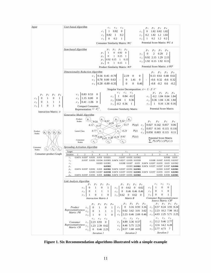
2.7 Illustration of the Six Collaborative Filtering Algorithms

We now use a simple hypothetical interaction matrix as input to illustrate the six

recommendation algorithms introduced above. In the left panel of Figure 1, we show the

interaction matrix and consumer-product graph representations of a simple transactional

recommendation dataset that involves 3 consumers, 4 products, and 7 observed

transactions (1’s in the matrix and links in the graph). The computational steps of the six

algorithms are shown on the right panels of Figure 1.

For the user-based and item-based algorithms, the consumer similarity matrix WC and

product similarity matrix WP are shown. The calculation follows the normalized

procedures described in [1] that take into account the global frequency of consumers and

products participating in transactions. The two resulting potential score matrices show

small difference but with similar patterns in rows and columns. For the dimensionality

reduction algorithm, the singular vector decomposition results are shown. We then show

the compact consumer representation based on a rank-2 approximation and the consumer

similarity matrix computed using the Cosine similarity function based on this compact

representation. For the generative model algorithm we specified the number of latent

classes to be 2 and present the estimates of the latent class probabilities P(z) and

conditional probabilities P(z|c) and P(z|p) on the latent class model. For the spreading

activation algorithm, we have shown the activation scores of the consumer/product nodes

of several iterations when each of the consumers is set as the starting node. Finally, for

the link analysis algorithm we show matrix B, the normalized version of the interaction

matrix A, and the matrix CR0. We then show the matrices PR and CR of the first three

iterations of computation. In this example, we did not perform the normalization at each

iteration to make it easy to follow the matrix multiplication calculations.

11

Link Analysis Algorithm

Spreading Activation Algorithm

Generative Model Algorithm

Dimensionality Reduction Algorithm

Item-based Algorithm

User-based AlgorithmInput

Consumer Similarity Matrix: WC

c 1 c 2 c 3

c 1 1 0.82 0c 2 0.82 1 0.2c 3 0 0.2 1

Potential Score Matrix: WC·A

p 1 p 2 p 3 p 4

c 1 0 1.82 0.82 1.82c 2 0.2 1.82 1.2 1.82c 3 1 0.2 1.2 0.2

Potential Score Matrix: A·WP

p 1 p 2 p 3 p 4

c 1 0 2 0.29 2c 2 0.92 2.15 1.29 2.15c 3 1.92 0.15 1.92 0.15

p 1 p 2 p 3 p 4

c 1 0.56 0.45 -0.70 2.19 0 0 0.13 0.61 0.48 0.61c 2 0.78 0.00 0.63 · 0 1.41 0 · -0.6 0.32 -0.6 0.32c 3 0.28 -0.89 -0.35 0 0 0.46 -0.8 -0.2 0.6 -0.2

Singular Vector Decomposition: A =

p 1 p 2 p 3 p 4

p 1 1 0 0.92 0p 2 0 1 0.15 1p 3 0.92 0.15 1 0.15p 4 0 1 0.15 1

Product Similarity Matrix: WP

c 1 c 2 c 3

c 1 1 0.84 -0.2c 2 0.84 1 0.36c 3 -0.2 0.36 1

Consumer Similarity Matrix

p 1 p 2 p 3 p 4

c 1 -0.2 1.84 0.64 1.84c 2 0.36 1.84 1.36 1.84c 3 1 0.16 1.36 0.16

Potential Score Matrix

c 1 0.83 0.53 0c 2 1.15 0.00 0c 3 0.41 -1.06 0

Compact ConsumerRepresentation: .

ProductNodes

ConsumerNodes

Latent Class

p3p1 p2 p4

z1 z2

c1 c2 c3

P(z)

P(z|c)

P(z|p)

0.77 0.23

0.34 0.090.47 0.30 0.19 0.61

0.110.24

0.37

0.020.20

0.57

0.320.17

Potential Score Matrix

p 1 p 2 p 3 p 4

c 1 0.027 0.142 0.057 0.06c 2 0.057 0.141 0.115 0.116c 3 0.058 0.003 0.115 0.11

Target:Iteration 1 2 3 4 5 1 2 3 4 1 2 3 4 5

c 1 0.0474 0.0207 0.0191 0.019 0.01831 0.0197 0.0191 0.01902 0.0186 0.019c 2 0.0197 0.0191 0.0194 0.01903 0.0474 0.0217 0.0195 0.01939 0.0188 0.0187 0.0193 0.01937c 3 0.0183 0.01901 0.0188 0.0187 0.019 0.0474 0.0207 0.0191 0.019 0.01902p 1 0.01903 0.0183 0.01865 0.0474 0.0197 0.0187 0.0187 0.01866p 2 0.0474 0.0197 0.0191 0.019 0.01902 0.0474 0.0197 0.0191 0.01903 0.0183 0.0187 0.01901p 3 0.0183 0.0187 0.01938 0.0474 0.0197 0.0191 0.01903 0.0474 0.0197 0.0191 0.019 0.01903p 4 0.0474 0.0197 0.0191 0.019 0.01865 0.0474 0.0197 0.0191 0.01903 0.0183 0.0183 0.01901

c 1 c 2 c 3

p 1 p 2 p 3 p 4

c 1 0 1 0 1c 2 0 1 1 1c 3 1 0 1 0

c 1 c 2 c 3

c 1 2.23 0.93 0c 2 1.23 2.39 0.62c 3 0 0.46 2.23

p 1 p 2 p 3 p 4

c 1 0 3.16 0.93 3.16c 2 0.62 3.62 3.01 3.62c 3 2.23 0.46 2.69 0.46

c 1 c 2 c 3

c 1 4.89 3.36 0.57c 2 4.46 5.75 2.23c 3 0.57 1.68 4.03

p 1 p 2 p 3 p 4

c 1 0.57 8.24 3.93 8.24c 2 2.23 10.2 7.98 10.2c 3 4.03 2.25 5.71 2.25

c 1 c 2 c 3

c 1 11.2 9.46 2.77c 2 12.6 14.2 6.28c 3 2.77 4.73 7

p 1 p 2 p 3 p 4

c 1 0 1 0 1c 2 0 1 1 1c 3 1 0 1 0

p 1 p 2 p 3 p 4

c 1 0 0.62 0 0.62c 2 0 0.46 0.46 0.46c 3 0.62 0 0.62 0

c 1 c 2 c 3

c 1 1 0 0c 2 0 1 0c 3 0 0 1

Interaction Matrix A Matrix B Consumer RepresentativenessSource Matrix: CR0

ProductRepresentativeness

Matrix: PR

ConsumerRepresentativeness

Matrix: CR

Iteration 1 Iteration 2 Iteration 3

Interaction Matrix: A

p 1 p 2 p 3 p 4

c 1 0 1 0 1c 2 0 1 1 1c 3 1 0 1 0

p4p3p2

c3c2

ProductNodes

ConsumerNodes

p1

c1

Consumer-product Graph

2/12ZU ⋅

'VZU ⋅⋅

∑zzpPczPcP )|()|()(

Figure 1. Six Recommendation algorithms illustrated with a simple example

12

An interesting comparison in this simple example involves the recommendation of

product p1 to consumer c1. The user-based and item-based algorithms only exploit the

direct consumer/product neighborhood information, thus both algorithms result in 0

potential score for the pair <c1, p1>. When exploring the transitive neighborhood

information, we can see that c3 can be considered as a transitive neighbor of c1 through a

common neighbor c2 and that p2 and p4 can be considered as transitive neighbors of p1

through a common neighbor p3. The other four algorithms indeed obtained non-zero

potential scores for <c1, p1>, showing their capability in capturing transitive associations

to make recommendations.

3. Evaluation of Recommendation Algorithms

Several previous studies have been devoted to evaluating multiple recommendation

algorithms [1, 4], but they mainly focused on variations of the user-based algorithms.

Furthermore, newly proposed algorithms are typically only compared with the user-based

algorithms. As a result, a comprehensive understanding of existing recommendation

algorithms’ performance is far from complete.

In our study, we selected 20% most recent interactions of each consumer’s

interactions to form the testing set and designated the remaining earlier 80% to be the

training set. To understand the performance of the algorithms under sparse data, we also

study recommendation performance with a reduced training set by randomly selecting

from the training set (referred to as the unreduced training set) only 40% of the

consumer’s total interactions. All the algorithms were set to generate a ranked list of

recommendations of K products. For each consumer, the recommendation quality was

measured based on the number of hits (recommendations that matched the products in the

testing set) and their positions in the ranked list. We adopt the following recommendation

quality metrics from the literature regarding the relevance, coverage, and ranking quality

of the ranked list recommendation (e.g., [1]):

(1) Precision: Pc = K

hitsofNumber ,

(2) Recall: Rc = set testingin the with interacted consumer products ofNumber

ofNumberc

hits ,

13

(3) F Measure: Fc = cc

cc

RPRP

+××2 , and

(4) Rank Score: ∑ −−=j hj

cjc

qRS )1/()1(2

, where j is the index for the ranked list; h is the

viewing half-life (the rank of the product on the list such that there is a 50% chance the

user will purchase that product); ⎩⎨⎧

= otherwise 0,

set, testings'in is if 1, cjqcj .

The precision and recall measures are essentially competing measures. As the number

of recommendation K increases, one expects to see lower precision and higher recall. For

this reason, the precision, recall, and F measures might be sensitive to the number of

recommendations. The rank score measure was proposed in [1] and adopted in many

follow-up studies (e.g., [3, 4, 6]) to evaluate the ranking quality of the recommendation

list. The number of recommendations has a similar but minor effect on the rank score, as

the rank score of individual recommendations decreases exponentially with the list index.

We also adopt a Receiver Operating Characteristics (ROC) curve-based measure to

complement precision and recall. Such measures are used in several recent

recommendation evaluation studies [4, 8]. The ROC curve attempts to measure the extent

to which a learning system can successfully distinguish between signal (relevance) and

noise (non-relevance). For our recommendation task, we define relevance based on

consumer-product pairs: a recommendation that corresponds to a transaction in the

testing set is deemed as relevant and otherwise as non-relevant. The x-axis and y-axis of

the ROC curve are the percent of non-relevant recommendations and the percent of

relevant recommendations, respectively. The entire set of non-relevant recommendations

consists of all possible consumer-product pairs that appear neither in the training set (not

recommended) nor in the testing set (not relevant). The entire set of relevant

recommendations corresponds to the transactions in the testing set. As we increase the

number of recommendations from 1 to the total number of products, a ROC can be

plotted based on the corresponding relevance and non-relevance percentages at each step.

The area under ROC curve (AUC) gives a complete characterization of the performance

of the algorithm across all possible numbers of recommendations. An ideal

recommendation model that ranks all the future purchases of each consumer at the top of

14

their individual recommendation list would expect to have steep increase in the beginning

and to flat out in the end, with AUC close to 1. A random recommendation model would

be a 45-degree line with AUC at 0.5.

For precision, recall, and F measure, an average value over all consumers tested was

adopted as the overall metric for the algorithm. For the rank score, an aggregated rank

score RS for all consumers tested was derived as ∑∑=

c c

c c

RSRS

RS max100 , where maxcRS was

the maximum achievable rank score for consumer c if all future purchases had been at the

top of a ranked list. The AUC measure was used directly as an overall measure for all

consumers.

4. An Experimental Study and Observations

We used three e-commerce datasets in our experimental study: a retail dataset provided

by a leading U.S. online clothing merchant, a book dataset provided by a Taiwan online

bookstore, and a movie rating dataset available from the MovieLens Project. The retail

dataset contained 3 months of transaction data with about 16 million transactions

(household-product pairs) involving about 4 million households and 128,000 products.

The book dataset contained 3 years of transactions of a sample of 2,000 customers. There

were about 18,000 transactions and 9,700 books involved in this dataset. The movie

dataset contained about 1 million ratings on about 6,000 movies given by 3,500 users

over 3 years. For the movie rating dataset we treated a rating on product p by consumer c

as a transaction (acp = 1) and ignored the actual rating. Such adaptation has been adopted

in several recent studies such as [3]. Assuming that a user rates a movie based on her

experience with the movie, we recommend only whether a consumer will watch a movie

in the future and do not deal with the question of whether or not she will like it.

For our experiments, we used samples from these three datasets. We included

consumers who had interacted with 5 to 100 products for meaningful testing of the

recommendation algorithms. This range constraint resulted in 851 consumers for the

book dataset. For comparison purposes, we sampled 1,000 consumers within this range

from the retail and movie datasets for the experiment. The details about the final samples

we used are shown in Table 1. In addition to the numbers of consumers, products and

15

transactions, we also report each dataset’s density level, which is defined as the

percentage of matrix elements valued at 1 in the interaction matrix. The movie dataset

has the highest density level (1.75%), followed by the book dataset (0.19%) and then the

retail dataset (0.13%). We also report the average number of purchases per consumer and

the average number of interacting consumers. The comparison among the three datasets

is consistent with the three density measures. The statistics of the complete datasets are

also reported in Table 1 in the parentheses.

Dataset # of Consumers

# of Products

# of Transactions

Density Level

Avg. # of purchases per

consumer

Avg. sales per product

Retail 1,000 (~4 million)

7,328 (~128,000)

9,332 (~16 million)

0.1273% (~0.0031%)

9.33 (~4)

1.27 (~125)

Book 851 (~2,000)

8,566 (~9,700)

13,902 (~18,000)

0.1907% (0.0928%)

16.34 (~9)

1.62 (~1.86)

Movie 1,000 (~3,500)

2,900 (~6,000)

50,748 (~1 million)

1.7499% (4.7619%)

50.75 (~166)

17.50 (~285.71)

Table 1. Characteristics of the datasets

Following the evaluation procedure described above, we prepared an unreduced

training set, a reduced training set, and a testing set for evaluation. Thus we had six

experimental configurations (3 datasets by 2 training sets) for each of the algorithms

under investigation. We set the number of recommendations to be 10 (K = 10) and the

half-life for the rank score to be 2 (h = 2). As for the algorithms examined, in addition to

the six collaborative filtering algorithms discussed above, we also included a simple

approach (referred to as the “Top-N Most Popular” or “Top-N” algorithm) that

recommends to a consumer the top 10 most popular unseen products as a comparison

benchmark.

Based on the existing literature and our understanding of the algorithms, we expect to

have the following findings: (1) Most algorithms should generally achieve better

performance with the unreduced (dense) dataset; (2) Algorithms that were specifically

designed for alleviating the sparsity problem should generally outperform the standard

correlation/similarity-based algorithms and the “Top-N” algorithm, especially for the

reduced (sparse) datasets; (3) The link analysis algorithm, with the global link structure

16

taken into consideration and a flexible control on penalizing frequent consumers and

products, is hypothesized to generally outperform other collaborative filtering algorithms.

Reduced Unreduced Reduced Unreduced Reduced UnreducedUser-based 0.0041 0.0088 0.0103 0.0202 0.0460 0.0648 4.17Item-based 0.0044 0.0096 0.0045 0.0091 0.0460 0.0759 4.50Dimensionality Reduction 0.0050 0.0064 0.0097 0.0191 0.0384 0.0530 5.50Generative Model 0.0069 0.0066 0.0283 0.0260 0.0377 0.0471 3.83Spreading Activation 0.0063 0.0130 0.0201 0.0231 0.0437 0.0607 3.67Link Analysis 0.0081 0.0133 0.0218 0.0267 0.0471 0.0624 1.67Top-N Most Popular 0.0069 0.0062 0.0268 0.0258 0.0373 0.0452 4.67User-based 0.0359 0.0663 0.0534 0.1041 0.0503 0.0686 4.33Item-based 0.0359 0.0711 0.0251 0.0454 0.0538 0.0864 4.33Dimensionality Reduction 0.0411 0.0408 0.0564 0.1026 0.0428 0.0580 5.17Generative Model 0.0429 0.0356 0.1616 0.1320 0.0382 0.0468 3.83Spreading Activation 0.0531 0.0863 0.1070 0.1155 0.0457 0.0618 3.33Link Analysis 0.0703 0.0891 0.1212 0.1282 0.0510 0.0649 2.17Top-N Most Popular 0.0429 0.0326 0.1553 0.1316 0.0377 0.0440 4.83User-based 0.0072 0.0153 0.0165 0.0320 0.0458 0.0634 4.33Item-based 0.0077 0.0166 0.0072 0.0142 0.0473 0.0769 4.17Dimensionality Reduction 0.0088 0.0109 0.0157 0.0305 0.0386 0.0528 5.33Generative Model 0.0113 0.0107 0.0454 0.0406 0.0362 0.0447 4.00Spreading Activation 0.0111 0.0219 0.0320 0.0362 0.0426 0.0583 3.67Link Analysis 0.0144 0.0224 0.0349 0.0415 0.0466 0.0605 1.83Top-N Most Popular 0.0113 0.0100 0.0431 0.0405 0.0357 0.0425 4.67User-based 1.8750 4.6519 3.8270 7.8635 4.5250 7.4500 4.17Item-based 2.0313 4.8527 1.0261 3.1281 4.2167 8.7500 4.33Dimensionality Reduction 3.4896 3.0120 3.0227 6.9486 4.1000 6.8000 5.17Generative Model 1.8490 1.4056 12.8120 10.7443 4.1250 5.1000 4.67Spreading Activation 3.7500 5.2209 8.6800 9.4955 4.7500 7.4000 3.00Link Analysis 4.4035 6.4074 9.9902 10.3835 5.3387 7.4319 2.00Top-N Most Popular 2.0052 1.3889 12.8397 10.7814 3.7000 5.0750 4.67User-based 0.4308 0.4628 0.3798 0.5287 0.7984 0.8544 5.67Item-based 0.4463 0.4810 0.3873 0.5558 0.8289 0.8930 4.33Dimensionality Reduction 0.4908 0.5663 0.5535 0.6894 0.8051 0.8602 3.00Generative Model 0.6166 0.6164 0.7246 0.7630 0.7849 0.8179 2.33Spreading Activation 0.4510 0.5194 0.4908 0.6569 0.7962 0.8325 4.67Link Analysis 0.4603 0.5852 0.6333 0.7462 0.7789 0.8058 3.83Top-N Most Popular 0.5296 0.5575 0.6487 0.7013 0.7772 0.8045 4.17

320 498 601 674 1000 1000

Measure AlgorithmDataset Avg.

Algorithm Rank

Retail Book Movie

Precision

Recall

F

Rank Score

Area Under ROC Curve

# of target consumers Table 2. Experimental results: performance measures

We report the five recommendation quality measures of the six experimental

configurations in Table 2. The boldfaced precision, recall, and F measures correspond to

the algorithms that were not significantly different from the highest measure in each

configuration at the 10% significance level. The boldfaced rank score and AUC measures

correspond to the best performing algorithm within each configuration. To provide a

summary of each algorithm’s overall performance across different datasets, we also

report the average rank of each algorithm across the six configurations. For example, for

the precision measure the link analysis algorithm’s average rank is 1.67, which

17

corresponds to the average of its ranks for individual configurations (1, 1, 3, 1, 1, and 3).

Boldfaced average ranks are the top average ranks. As collaborative filtering algorithms

can only recommend products that appeared in the training transactions, for consumers

who do not have recommendable products in the testing set no successful

recommendation is possible. To make the performance measures meaningful, we only

evaluate recommendations for target consumers for whom successful recommendations

are possible. Therefore, for the same dataset the reduced and unreduced training sets had

different numbers of target consumers, which are reported in the bottom of Table 2.

Precision Relative to Top-N Most Popular

0

0.5

1

1.5

2

2.5

retailreduced

retailunreduced

bookreduced

bookunreduced

moviereduced

movieunreduced

Recall Reltative to Top-N Most Popular

0

0.5

1

1.5

2

2.5

3

retailreduced

retailunreduced

bookreduced

bookunreduced

moviereduced

movieunreduced

F Measure Relative to Top-N Most Popular

0

0.5

1

1.5

2

2.5

retailreduced

retailunreduced

bookreduced

bookunreduced

moviereduced

movieunreduced

Rank Score Relative to Top-N Most Popular

0

0.5

1

1.5

2

2.5

3

3.5

4

4.5

5

retailreduced

retailunreduced

bookreduced

bookunreduced

moviereduced

movieunreduced

User-based Item-based Dimensionality ReductionGenerative Model Spreading Activation Link AnalysisTop-N Most Popular

Figure 2. Experimental results: performance measures relative to the Top-N algorithm

For easy visualization of the results, we present in Figure 2 the relative precision,

recall, F, and rank score measures of the individual algorithms computed as the actual

measures divided by those corresponding measures obtained by the “Top-N” algorithm.

For example, the link analysis algorithm’s value in the precision diagram for the

unreduced retail dataset was 2.13, meaning its precision was 113% higher than that

achieved by the “Top-N” algorithm.

18

In Figure 3 we present the AUC measures of each algorithm across the six

configurations. We also show the actual ROC curves for the unreduced and reduced retail

dataset as examples.

Area Under ROC Curve

0.3000

0.4000

0.5000

0.6000

0.7000

0.8000

0.9000

1.0000

retail reduced retailunreduced

book reduced bookunreduced

movie reduced movieunreduced

User-based Item-based Dimensionality Reduction Generative ModelSpreading Activation Link Analysis Top-N Most Popular

Figure 3. AUC measures and the ROC curves for the retail dataset

Based on these results we report the following observations.

• All algorithms achieved better performance with the unreduced data. The

performance measures shown in Table 2 were generally better with the unreduced

datasets than with the reduced datasets. The difference is even more significant

when the numbers of target consumers are taken into account. For example, the

average precision measure of 0.81% for 320 target consumers under the reduced

retail dataset should be adjusted to 0.52% (0.81%×320/498) when compared with

the average precision of 1.33% for 498 target consumers under the unreduced

dataset. The general upward pattern for lines in Figures 2 and 3 visually

19

demonstrates this finding. There were only 4 exceptions in the total of 105 data-

algorithm-measure configurations after the effect of the number of target

consumers is adjusted: the recall and rank score measures of the Top-N algorithm

under the reduced book dataset are slightly higher than their counterparts under

the unreduced book dataset; the recall and rank score of the generative model

algorithm under the reduced book dataset are slightly higher than its counterpart

under the unreduced book dataset.

• The link analysis algorithm generally achieved the best performance across all

configurations except for the movie dataset. Table 2 shows that the link analysis

algorithm achieved the highest average ranks for the precision, recall, F, and rank

score measures (1.67, 2.17, 1.83, and 2). The spreading activation algorithms

achieved the second highest average ranks (3.67, 3.33, 3.67, and 3). The average

ranks for all other algorithms were between 4 and 6. The good performance of

both the link analysis and spreading activation algorithms seems to indicate that

additional valuable information (such as transitive associations) in sales

transactions can be effectively exploited by graph-based algorithms. The link

analysis algorithm’s dominance over other algorithms was most evident with the

unreduced retail datasets. It achieved about 150% higher precision, recall, and F

measures and a more than 350% higher rank score than the Top-N algorithm.

• The AUC measure generally reveals different comparison results from the other

four measures. The generative model algorithm achieved the best AUC measures

for the reduced retail dataset and the book datasets. The link analysis algorithm

achieved best AUC measures for the unreduced retail datasets. The item-based

algorithm achieved the best AUC measures for the movie datasets. The generative

model algorithm achieved the best average rank of 2.33. The ROC curves provide

a complete characterization of the algorithm performance for all possible numbers

of recommendation increases. However, the AUC measure only provides an

overall summary of an algorithm’s performance, which does not necessarily

correspond to its performance in practical recommendation settings. For example,

the consumers are typically much more interested in the quality of the top 10

recommendations and the performance of the algorithm at the 100th to 1000th

20

recommendations is practically irrelevant. Take the ROC curves for the

unreduced retail dataset in Figure 3 as an example. The ROC curves for the link

analysis algorithm and the generative model algorithm showed comparable

performance, which correspond to the similar AUC measure in Table 2 (0.5852

and 0.5663, respectively). However, a more meaningful comparison is the fact

that the ROC curve of the link analysis algorithm was much steeper than that of

the generative model algorithm at the beginning, which corresponds to the

significantly higher precision and recall measures than those obtained by the

generative model algorithm (0.0133 and 0.0891 as compared to 0.0066 and

0.0356, respectively).

• Most other algorithms showed mixed performances under different datasets. The

item-based algorithm performed exceptionally well for the movie datasets, but

had relatively lower quality with the retail datasets and the worst performance

with the book dataset. The good performance of the item-based algorithm with the

movie dataset may be associated with the datasets’ much higher transaction

density levels (1.75%) and average sales per product (17.50) than other datasets.

The dimensionality reduction algorithm consistently achieved a mediocre

performance across all configurations and the user-based algorithm was almost

always dominated by other algorithms. The generative model algorithm always

achieved comparable but better performance than the Top-N most popular

algorithm, with relatively good performance with the book datasets and the

reduced retail dataset but the worst performance with the movie datasets and the

unreduced retail dataset.

• An interesting observation from our experimental results is that the Top-N

algorithm was not necessarily a low-performing algorithm for many

configurations despite its simplicity. This is especially the case for the book

dataset. On the other hand, a closer examination of the actual recommendations

made by various algorithms showed that a large portion of the collaborative

filtering recommendations were different from those given by the Top-N

algorithm. Collaborative filtering-based recommendations therefore still provide

21

value to consumers, complementing simple popularity-based recommendations

such as those made by the Top-N algorithm.

0

0.5

1

1.5

2

2.5

3

3.5

4

4.5

5

User-based Item-based DimensionalityReduction

GenerativeModel

SpreadingActivation

Link Analysis

log 1

0(to

tal c

ompu

tatio

n tim

e in

sec

onds

)

Figure 4. Computational efficiency analysis

We now report the empirical computational efficiency of these recommendation

algorithms under study using the unreduced retail dataset as the testbed. Figure 4

summaries total computing times of all algorithms. (All algorithms were implemented in

Python, a common scripting language (www.python.org), for fast prototyping. We expect

that a 10-50 speed-up factor can be achieved when using a more efficient implementation

environment such as the C programming language.) The dimensionality reduction

algorithm required the longest running time. This was because after reduction the

interaction matrix becomes dense and pair-wise consumer similarity computation

required significant CPU cycles. The Item-based algorithm was slow due to the large

number of products (relative to the number of consumers) in the dataset. Both the

spreading activation and link analysis algorithms required only a small number of

iterations to achieve satisfactory recommendation quality, thus requiring modest

computing times (less than that required of the item-based algorithm). The spreading

activation algorithm was especially fast because it computes recommendations for target

consumers only as opposed to computing recommendations for all consumers in a batch

mode. The generative model in general is very efficient mainly because (a) a small

number of hidden classes are required for quality recommendations and (b) the maximum

likelihood estimation procedure converges very fast.

22

5. Conclusion and Future Research

A unique contribution of the reported study is a comprehensive evaluation of a wide

range of collaborative filtering algorithms using transactional e-commerce datasets.

Although our link analysis-based algorithm introduced in this article achieved the best

overall performances, no single algorithm was observed to dominate other algorithms

across all experimental configurations.

From a practical standpoint, our study points to the need of developing a meta-level

guideline that “recommends” an appropriate recommendation algorithm based on the

characteristics of the available data in specific application settings. Based on our

experimental findings, although the overall sparsity level and the row/column density of

the consumer-product interaction matrix have some clear influence over the relative

performance of selected algorithms, such data characteristics are far from complete and

lack predictive power as a foundation for the discussed meta-level guideline. Additional

prescriptive descriptors of the interaction data clearly need to be developed. We expect

that these descriptors should include measures from graph/network topological modeling

literature, such as node degree distribution, average path length, and cluster coefficient.

Our ongoing research is exploring the customized versions of these descriptors for

recommendation analysis and using them to guide further comparative evaluations of

various recommendation algorithms.

6. Acknowledgement The reported research was partly supported by an NSF Digital Library Initiative-II grant,

“High-performance Digital Library Systems: From Information Retrieval to Knowledge

Management,” IIS-9817473, April 1999 – March 2002, and by an NSF Information

Technology Research grant, “Developing a Collaborative Information and Knowledge

Management Infrastructure,” IIS-0114011, September 2001 – August 2005. The link

analysis algorithm studied in this article was originally reported in a conference paper

presented at the Tenth Annual Americas Conference on Information Systems (AMCIS

2004). The second author is also affiliated with The Key Lab of Complex Systems and

Intelligence Science, Chinese Academy of Sciences (CAS), Beijing, and was supported in

part by a grant for open research projects (ORP-0303) from CAS.

23

7. References 1. Breese, J.S., Heckerman, D. and Kadie, C., Empirical analysis of predictive

algorithms for collaborative filtering. in Fourteenth Conference on Uncertainty in Artificial Intelligence, (Madison, WI, 1998), Morgan Kaufmann., 43-52.

2. Brin, S. and Page, L., The anatomy of a large-scale hypertextual Web search engine. in 7th International World Wide Web Conference, (Brisbane, Australia, 1998).

3. Deshpande, M. and Karypis, G. Item-based top-N recommendation algorithms. ACM Transactions on Information Systems, 22 (1). 143-177, 2004.

4. Herlocker, J.L., Konstan, J.A., Terveen, L.G. and Riedl, J.T. Evaluating collaborative filtering recommender systems. ACM Transactions on Information Systems, 22 (1). 5-53, 2004.

5. Hofmann, T. Latent semantic models for collaborative filtering. ACM Transactions on Information Systems, 22 (1). 89-115, 2004.

6. Huang, Z., Chen, H. and Zeng, D. Applying associative retrieval techniques to alleviate the sparsity problem in collaborative filtering. ACM Transactions on Information Systems (TOIS), 22 (1). 116-142, 2004.

7. Kleinberg, J., Authoritative sources in a hyperlinked environment. in ACM-SIAM Symposium on Discrete Algorithms, (San Francisco, CA, 1998), ACM Press, 668-677.

8. Papagelis, M., Plexousakis, D. and Kutsuras, T., Alleviating the sparsity problem of collaborative filtering using trust inferences. in 3rd International Conference on Trust Management (iTrust 2005), (Paris, France, 2005), 224-239.

9. Resnick, P., Iacovou, N., Suchak, M., Bergstorm, P. and Riedl, J., GroupLens: An open architecture for collaborative filtering of netnews. in ACM Conference on Computer-Supported Cooperative Work, (1994), 175-186.

10. Resnick, P. and Varian, H. Recommender systems. Communications of the ACM, 40 (3). 56-58, 1997.

11. Sarwar, B., Karypis, G., Konstan, J. and Riedl, J., Application of dimensionality reduction in recommender systems: a case study. in WebKDD Workshop at the ACM SIGKKD, (2000).

12. Ungar, L.H. and Foster, D.P., A formal statistical approach to collaborative filtering. in CONALD'98, (1998).