Recent Progress in Inverse Problems inElectrocardiology

Robert S. MacLeod∗ and Dana H. Brooks†

Short titles: Inverse Problems in ElectrocardiologyAddress for correspondence: Dr. Robert S. Macleod, Nora Eccles Harrison CVRTI,

Building 500, University of Utah, Salt Lake City, Utah.Telephone: (801)581-8183, FAX: (801)581-3128,Email: macleod@cvrti.utah.edu.

Support: Richard A. and Nora Eccles Harrison Treadwell Fund for Cardiovascular Research andawards from the Nora Eccles Treadwell Foundation. National Institutes of Health SCOR inSudden Cardiac Death, HL 52338-01. National Science Foundation under Grant No. BCS-9309359,

∗Nora Eccles Harrison Cardiovascular Research and Training Institute, University of Utah, Salt Lake City, Utah†CDSP Center, ECE Dept, Northeastern University, Boston, Massachusetts

1

Introduction

The ultimate, if utopian, use of electrocardiography would be to describe the electrochemical

activity of each cell in the heart based on body surface electrocardiograms (ECGs). Currently,

in everyday practice, clinicians use the ECG to diagnose the health of a patient’s heart based

on a current dipole model of the cardiac electrical source. This diagnosis is typically qualitative

rather than quantitative, and based more on empirical pattern recognition than on biophysical

modeling. On the other hand, it is also performed in almost real time, and is amenable to the

use of other clinical variables to constrain and confirm the resulting diagnosis. Both the utopian

and the clinical use of the ECG require solutions to the inverse problem of electrocardiography,

and they represent the two extremes among the many formulations of this problem. There are

a number of useful formulations in between, more comprehensive and quantitative than current

clinical practice; multichannel ECG measurements (“body surface potential maps”) along with a

mathematical model of cardiac bioelectric sources are used to describe macroscopic cardiac electrical

activity by estimating the values of the modeled sources. The purpose of this paper is to review

recent progress in such electrocardiographic inverse problems.

Solving the electrocardiographic inverse problem is made difficult by two characteristics it shares

with many other scientific and engineering inverse problems. The first characteristic is the non-

unique relationship between the true intra-cardiac sources and our remote observations—the same

set of measurements could result from more than one source configuration. To accommodate this,

we seek inverse problem formulations that have unique source models, and accept as a consequence

the possible loss in generality, applicability, and ability to validate. The second troublesome char-

acteristic is the ill-posedness of the inverse problem resulting from attenuation (due to dissipation)

and smoothing (due to spatial superposition) of the electric fields in the medium between source and

observation. Recovering the sources from the resulting remote measurements requires amplification

and “unsmoothing”. When applied to measurements contaminated with unavoidable noise, while

2

using models with unavoidable model error, the result can be large, nonlinear, even discontinuous

errors in inverse solutions. In the discussion that follows, we outline several approaches to mitigate

these difficulties.

The field of inverse electrocardiography was summarized comprehensively in 1988-89 in a series

of reviews by Rudy and Messinger-Rapport [1, 2] and Gulrajani, et al. [3–6]. These papers describe

methods that solved the basic problem, but produced results that were notoriously unreliable and

their significance, in either research or clinical contexts, was not convincingly established. Research

in the intervening years has focused on such topics as increasing robustness to discretization error

and model assumptions, maximizing use of available a priori information, formulating the inverse

problem in ways that reduce ambiguity and increase utility of the results, removing obstacles to

clinical application, and carefully validating solution methods. More recent reviews and tutorials

by Horacek [7], Greensite [8], and Rudy [9] have covered a few of the developments in the field.

Here we emphasize a more comprehensive view of important recent results and the current state of

the field. We apologize in advance for omissions due to space constraints and oversight.

Problem formulations

There are three requirements that govern formulations of an inverse problem in electrocardiology:

1) posing a problem that has a well-defined solution, 2) describing this problem in a form that

facilitates the use of reasonable numerical techniques, and 3) defining source model and observation

locations that permit measurements under physiological conditions. The two classes of formulations

described in this section meet these conditions and, therefore, have emerged from a broad collection

of alternatives as the most promising approaches. These two alternative formulations are based on

different “equivalent representations” of the intra-cardiac sources. Each source representation then

leads to a particular set of equations, solved by one or more numerical techniques. We omit any

discussion of inverse problems based on discrete intra-cardiac dipole source models, as the coverage

of this topic in [3] is still contemporary.

3

Solutions in terms of potential distributions

The more general of these formulations represents the actual intra-cardiac sources in terms of

the distribution of electrical potential on a closed surface that completely separates the sources

from the observations [10]. The field anywhere on the observation side of such a surface has, in

principle, a one-to-one association with the potential distribution on the surface itself. Thus the

potential distribution on this surface represents an equivalent source. For example, one such ideal

surface is the epicardium, the outer surface of the heart, with the measurements made on the body

surface. In addition to providing a theoretically unique solution, epicardial potentials can be—and,

in fact, often are [11–13]—measured using invasive techniques. Thus they provide both a useful

clinical description of cardiac electrical activity as well as a practical validation mechanism for

inverse solutions.

The resulting mathematical formulation of the problem requires solving Laplace’s equation for

the region between the epicardial and torso surfaces, denoted as ΓE and ΓT respectively, i.e.,,

∇ · (σ∇φ) = 0 in Ω, (1)

with the appropriate Dirichlet

φ = φ0 on ΓE (2)

and Neumann

(σ∇φ) · n = 0 on ΓT (3)

boundary conditions, where φ is the potential anywhere in the volume Ω bounded by the surfaces

ΓE and ΓT , σ is the conductivity, and n is the outward surface normal.

A second variant of the potential distribution formulation takes advantage of our ability to mea-

sure potentials measured with an intracavitary probe introduced surgically, or even percutaneously

via catheter, into one of the heart’s chambers [14, 15]. Here the bounding surface representing

the source is the endocardium (the inner surface of the heart); the measurement probe provides

4

the Neumann boundary and the endocardial surface the Dirichlet boundary. This formulation is

of great clinical interest because it offers the possibility of rapid and comprehensive endocardial

mapping during ablation procedures.

Solutions in terms of activation wavefronts

During the spread of activation in the heart, the most significant bioelectric source is the large

potential difference that exists across the moving wavefront that divides active (depolarized) from

resting tissue. Thus investigators have developed source representations leading to tractable inverse

problems that directly model this wavefront [16, 17]. One starts by assuming that the extracardiac

field during activation can be approximated as the field produced by a uniform double layer of

current dipoles (UDL) lying along the activation wavefront and oriented in the normal direction.

This wavefront is accessible only to electrodes mounted within the heart tissue—thus we need a more

convenient equivalent source. Because the external field from a UDL is a function of the solid angle

swept out by the boundaries of the excited region, we can replace the actual activation wavefront

by any UDL that has the same solid angle. The most convenient choice of equivalent UDL is the

surface that lies on the boundary of the heart and encloses all currently excited tissue. The moving

edge of this surface is defined by the time at which the underlying tissue becomes depolarized

(the “activation time”) and its full extent is the union of the epicardium and endocardium, made

continuous by a small fictional adjoining segment near the base of the heart. The simplifying

assumptions of the UDL—the constant voltage step across the wavefront and normal direction of

the dipole moment—permit a further simplification of the extracardiac field:

φ(y) =

∫Sv

T (y, x)H(t − τ(x))dSx, (4)

where φ(y) is the potential at extracardiac site y, H is the Heaviside step function, τ(x) is the time

at which each portion of the epi/endocardium (Sv) becomes depolarized (the activation time) and

T (y, x) is a transfer function that weights the contribution of each point of the cardiac surface x

5

to each point on the torso surface y [16, 17].

A pictorial summary of the three formulations described here is shown in Fig. 1.

Please place Figure 1 here

Discussion

One strength of the potential based formulations is that they are more general—they recover

the potential anywhere on the surface or within the appropriate volume conductor at any point in

the cardiac cycle. The UDL method, by contrast, only recovers the activation wavefronts (QRS

complex) and gives no information about repolarization or recovery (ST segment and T wave).

In addition, the UDL method requires the assumption of a uniform dipole layer, implying that

the wavefront does not reflect the effects of anisotropic conduction. Many experimental studies

have shown that such an assumption is incorrect [18–20], but the effect of this discrepancy on

the inverse problem is a topic of current research [21, 22]. Thus the assumptions implicit in the

potential based formulations are less restrictive, and the solutions may contain more information.

However, potential formulations are over-parameterized to some extent—they do not take explicit

advantage of the “wavefront” behavior (spatio-temporal coherence) which characterizes important

aspects of cardiac electrical activity. As a result of its more parsimonious representation, the UDL

formulation tends to be less ill-posed. Moreover, the activation wavefront trajectory has relatively

clear physiological meaning and is an immediately useful result, while solutions in terms of potentials

are more ambiguous and require further processing even to obtain activation wavefronts [23].

Modeling considerations

All the methods described above share certain common assumptions: quasi-static propagation,

temporally constant geometry (questionable during recovery), a torso which is homogeneous or

divided into piecewise homogeneous compartments with known relative conductivities, a linear

medium, potentials that are recorded with respect to a common reference, and insignificant non-

6

cardiac electrical activity. Given these assumptions, Bayley, et al., [24] and then later Rudy, et al.,

[25–27] developed elegant analytical inverse solutions based on concentric and eccentric spheres and

used them to investigate many aspects of the forward and inverse problems. Barr, et al., [28, 29] and

Colli-Franzone, et al., [30, 31] incorporated realistic torso geometries into discrete forward/inverse

solutions based on the epicardial potential formulation. Barr, et al., applied a Green’s theorem

approach to the formulation in equations 1–3 and then used the boundary element method (BEM)

to describe and solve the resulting integral equations. Colli-Franzone, et al., and later Yamashita,

et al. [32], on the other hand, employed a Galerkin formulation and the finite element method

(FEM). The BEM and FEM remain the main numerical approaches and their relative merits have

been well discussed in [2]. The UDL formulation of the inverse problem leads directly to surface

integral equations and hence has been solved exclusively using the BEM, most notably by Huiskamp

and van Oosterom [17].

The final result of all these approaches is a forward solution, a simple description of the relation-

ship between sources and remote body-surface or probe-surface potentials. For the epicardial to

body surface formulation, for example, we have

φb(y) = Z(y, x)φh(x), (5)

where φb and φh are body surface and epicardial potentials, respectively and Z(y, x) is a transfer

function weighting the contribution of each epicardial site to the potential at each body surface

site.

The geometric models required by both BEM and FEM for realistic inverse problems include a

discrete set of points, linked to form a three-dimensional mesh and segmented into regions of locally

constant conductivity. Notable landmarks in mesh generation research include the early results of

van Oosterom on surface triangulation techniques based explicitly to the BEM method [33], and

more recent progress by Johnson, MacLeod, Schmidt, and coworkers [34–37] on segmentation and

tetrahedral mesh generation. The latest programs are capable of creating meshes with over one

7

million elements based on magnetic resonance imaging of human subjects. Early inverse solutions

assumed homogeneous conditions throughout the volume conductor [28]. Many subsequent mod-

eling studies have attempted to determine the influence of conductivity inhomogeneities on the

inverse solution and Gulrajani has discussed their often contradictory conclusions [5]. The last ten

years have seen relatively little resolution of this issue, although recent simulation studies with a

three-dimensional forward solution using an elaborate geometrical model suggest that omission of

subcutaneous fat, anisotropic skeletal muscle, and, to a lesser extent, the lungs cause the largest

errors in forward solutions [38]. Experimental studies have revealed that variation in torso conduc-

tivity affects not only body surface potentials but also the potential distributions recorded on the

epicardium [39–41].

Improvements in numerical techniques to solve forward/inverse problems have generally been

restricted to specific problem formulations. For example, better numerical techniques have been

applied to the integrations required for BEM solutions, moving from assumptions of constant

potential over each element [28] to triangle subdivision schemes [42, 43], to linear variation over

each element [2, 44]. Adaptive mesh refinement, a process by which selected elements of the mesh

are subdivided or merged based on local error estimates, has been applied so far only to FEM

models [45, 46]. A potentially powerful approach is to combine the strengths of both the BEM

and FEM and apply them to different subdomains of the mesh [47]. One issue which has recently

emerged is whether meshes which may be optimal for forward solutions are also optimal for inverse

solutions: results indicate that in fact this may not be the case [48].

Solving the inverse problem

Given the ill-posed nature of the inverse problem, the ambiguities of various source models,

the errors in any forward solution, and the presence of noise in measured data, the formulation

of a useful inverse model does not follow directly from the source models and forward solutions

described so far. One needs to find a way to select the best solution from the available information;

8

even the way that one chooses to define “best” can have a significant effect on the answer. The

most straightforward way is to look for the solution that minimizes the difference between the torso

measurements predicted by a candidate solution together with the forward model, on the one hand,

and the actual measured data on the other hand. This difference, known as the residual error, is

usually measured in terms of sum-squared error (or ℓ2 norm). The effect of the ill-posedness of the

inverse problem is that solutions which simply minimize this residual error will be unreliable and

often unrealistic—consequently, a more sophisticated approach is required.

The standard response to this ill-posedness is known as regularization: a weighted sum of two

terms is minimized. One term is the residual error and the other is a penalty term describing

an undesirable property of the solution. The most common example of such penalty terms are

the ℓ2 norm of the solution, penalizing for excessive amplitude, or the ℓ2 norm of its first or

second (spatial) derivative, penalizing for lack of smoothness. The chosen undesirable property

acts as a constraint on the solution, reducing the extreme sensitivity of the ill-posed minimum

residual result. The constraint then becomes a way to incorporate into the inverse model a priori

information about how a reasonable solution should behave. A weighting parameter, known as

the “regularization parameter,” is used to control the tradeoff between the two error terms. There

is a rich literature about regularization, both generally in applied mathematics [49–52] as well

as specifically in inverse electrocardiography, and these methods can be interpreted in terms of

physics, linear algebra, complexity theory, information theory, statistics, image processing, and

other fields. Moreover, ℓ2 norm based regularization is not the only way to approach the problem.

For instance, in earlier work by Brooks and collaborators, the inverse problem was posed in the

power spectrum domain [53]; in this context other error measures, such as relative entropy, are

available. Thus, solving the inverse problem is not merely a question of numerical implementation,

but rather one of choosing the appropriate principle upon which an optimal or acceptable inverse

solution will be judged, and one can use entirely different principles than constrained squared error,

9

i.e.,, regularization, to construct error functions to minimize.

The general result of the application of regularization methods to electrocardiography between

the mid 1970’s and the late 1980’s was, as described above, only partially satisfactory. Two possible

approaches to improving this result are to 1) reduce the various sources of error and 2) incorporate

more a priori information. We will not discuss results from the considerable research utilizing the

former approach (see, for example, [34, 46, 54, 21, 55]). We see recent work on the latter approach as

generally having followed three main paths: 1) explicitly including more information by using novel

constraints, or more than one constraint, 2) implicitly including more information by formulating

the source model based on a characterization of the dynamics of cardiac electrical activity, thereby

effectively restricting the solution domain, and 3) using the constraints in a “smarter,” “tuned”

manner. A number of methods cross the boundaries of these somewhat artificial categories, but we

will use this scheme to delineate the major approaches we describe below.

Using novel and/or multiple constraints

There have been two general trends in this category: using other constraints besides the tra-

ditional amplitude and spatial derivative ℓ2 norms, and using more than one constraint. Specific

examples include orthogonality constraints [56], constraints on the normal component of current on

the epicardial surface [57], and explicit constraints on the temporal behavior of solutions [58–63].

Much attention has been given to methods that incorporate more than one constraint, particularly

temporal and spatial constraints. Oster and Rudy employed a two-step method to take advantage

of presumed temporal continuity of solutions [58]; first spatially regularized solutions were calcu-

lated, then these solutions were “temporally regularized” to constrain nearby temporal samples at

a particular epicardial location to be reasonably close to each other. Effectively this amounted to

a temporal “post-filtering” operation on the spatial regularization. Brooks, et al., incorporated a

number of time instants into an “augmented” formulation of the problem, and then found a solution

which jointly minimized a combination of three terms: the residual error, a spatial constraint error,

10

and a temporal constraint error. El-Jakl, et al., [62] proposed a Kalman filter solution to essentially

the same problem. Greensite [63] has recently introduced a method based on a doubly Truncated

Singular Value Decomposition (TSVD) regularization which uses information about the interaction

between “temporal” and “spatial” subspaces which depend on the temporal correlation of the data,

and the inner product of the forward solution over the heart surface, respectively. Brooks, et al.,

extended the time/space constraint approach to include first dual spatial constraints [64], and then

later also a truncated conjugate gradient-type regularization [60]. Shahidi, et al., combined two

spatial constraints by means of a hybrid regularization term which merged a TSVD approach with

an explicit constraint on the solution norm [65]. In general, combining constraints seems to produce

results that are less sensitive to the choice of constraint and less sensitive to the choice of regu-

larization parameters or truncation index. In addition, the incorporation of temporal information

produces a much more realistic behavior of the reconstructed time signals (electrograms), without

apparent loss of accuracy of spatial distributions.

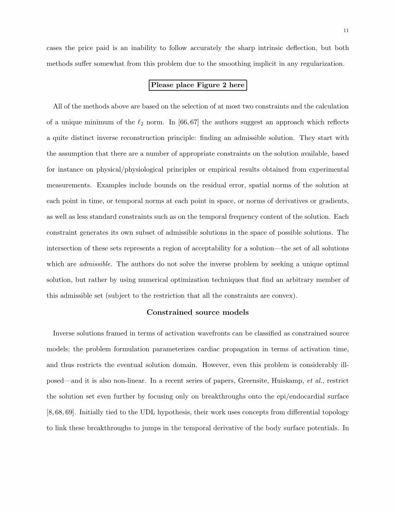
Figure 2 shows a sample comparison of standard spatially regularized results to those achieved

using the joint time/space regularization method described in [61]. The results are computed by first

applying a forward solution to measured epicardial electrograms from an isolated heart to generate

simulated torso surface ECGs, as described in the Validation section below. After adding noise to

the simulated torso signals, we computed inverse solutions with a variety of regularization techniques

and parameters. In the figure, sixty millisecond long segments of electrograms during QRS are

shown for four different locations on the epicardium. The first and third rows show results using

spatial regularization only, and the second and fourth rows using additional temporal regularization.

Each plot shows the original measured electrogram as a solid line and reconstructions at various

regularization parameters (or pairs of regularization parameters for the joint time/space method).

Notable in the joint time/space results is the decreased sensitivity to variation of the regularization

parameter values and significant decrease in unrealistic uncorrelated temporal behavior. In some

11

cases the price paid is an inability to follow accurately the sharp intrinsic deflection, but both

methods suffer somewhat from this problem due to the smoothing implicit in any regularization.

Please place Figure 2 here

All of the methods above are based on the selection of at most two constraints and the calculation

of a unique minimum of the ℓ2 norm. In [66, 67] the authors suggest an approach which reflects

a quite distinct inverse reconstruction principle: finding an admissible solution. They start with

the assumption that there are a number of appropriate constraints on the solution available, based

for instance on physical/physiological principles or empirical results obtained from experimental

measurements. Examples include bounds on the residual error, spatial norms of the solution at

each point in time, or temporal norms at each point in space, or norms of derivatives or gradients,

as well as less standard constraints such as on the temporal frequency content of the solution. Each

constraint generates its own subset of admissible solutions in the space of possible solutions. The

intersection of these sets represents a region of acceptability for a solution—the set of all solutions

which are admissible. The authors do not solve the inverse problem by seeking a unique optimal

solution, but rather by using numerical optimization techniques that find an arbitrary member of

this admissible set (subject to the restriction that all the constraints are convex).

Constrained source models

Inverse solutions framed in terms of activation wavefronts can be classified as constrained source

models; the problem formulation parameterizes cardiac propagation in terms of activation time,

and thus restricts the eventual solution domain. However, even this problem is considerably ill-

posed—and it is also non-linear. In a recent series of papers, Greensite, Huiskamp, et al., restrict

the solution set even further by focusing only on breakthroughs onto the epi/endocardial surface

[8, 68, 69]. Initially tied to the UDL hypothesis, their work uses concepts from differential topology

to link these breakthroughs to jumps in the temporal derivative of the body surface potentials. In

12

the latter papers they attempt to remove the dependence on the UDL assumption. In another,

related, approach, they use a subspace-based argument to detect timing of breakthroughs by means

of the sudden appearance of an “independent source,” causing a change in the distance between

two subspaces, as they search both forward and backward in time through the QRS [70]. Once the

breakthrough times have been located, they find the breakthrough locations and, finally, use these

“high-quality” estimates of the breakthroughs and a regularization approach to find the rest of the

isochronal distribution.

Tuned application of constraints

Another approach to improved accuracy and reliability in recent inverse problem research has

been to use a priori information to apply constraints in a more effective manner. One such ap-

proach introduced by Johnson, et al., factors an FEM forward solution into distinct matrices,

each representing the relationship between two volume compartments in the model [54]. Some

of these submatrices are considerably better conditioned than others, suggesting that the related

“sub-inverse problems”, as it were, are better posed. Thus the regularization can be tuned by only

applying it to each submatrix as needed. A quite different approach introduced by Iakovidis and

Gulrajani is based on the observation that over-regularization produces overly smooth solutions

that are not very accurate around extrema but reasonably reliable where amplitudes are small[71].

In an analogous fashion, solutions with less regularization than optimal locate maxima and minima

reasonably accurately, but produce very noisy reconstructions in other locations. Therefore, the

authors constrained the inverse solution in small amplitude regions to agree with an overregular-

ized solution, constrained the extremal locations according to an underregularized solution, and the

remainder by the standard regularization criteria. This approach can be thought of as an attempt

to adjust the amount of regularization to match the local Signal-to-Noise Ratio (SNR): where the

SNR is high, only regularize a little, and where it is low, regularize a lot. Messinger-Rapport and

Rudy, in [72], suggest an approach using constrained optimization techniques to impose constraints

13

such as a maximum value on the solution. Oster and Rudy describe a spatially varied regularization

scheme [73] applied to concentric (and then eccentric) spheres, in which they use Legendre polyno-

mials (and then the SVD) to delineate a sequence of orthogonally decomposed sub-reconstructions.

Different regularization parameters are used to weight different terms in this decomposition; the

idea is that the local SNR should guide the local degree of regularization. The admissible solutions

work described above also included the use of spatially weighted constraints. Here the weighting

of individual constraints varied spatially based on some a priori knowledge of the expected ampli-

tude of constraint-specific properties. Thus, for example, where potential amplitudes are small an

ℓ2 norm constraint will be emphasized, while where they are large it will be downweighted, since

this constraint by itself generally allows too much low-amplitude noise but smoothes the largest

amplitudes. All these methods produce an increase in the accuracy and reliability of their inverse

solutions over more straightforward regularization schemes.

Validation and Clinical Applications

In this section, we explicitly return to the theme of this special issue and discuss the link between

the theory and numerics of the inverse problems and the techniques of multichannel data acquisition

and processing. The input signals for any electrocardiographic inverse solution come from electrodes

placed on the body surface or mounted in a probe that is inserted into the ventricle, with sufficient

density and coverage to represent adequately the entire surface potential distribution. The practical

interpretation of “sufficient density” is a point of considerable debate, reflected in the range of

electrode numbers used in typical body surface potential mapping systems, between 32 and 200.

(In fact, the theoretical claim made above of a unique one-to-one relationship between surface

potential distributions is in fact only true if the entire distribution of potential on the surfaces is

known.) Unlike the more common issue of temporal sampling, with spatial sampling it is difficult

to apply Shannon sampling theory due to uncertainty about actual spatial frequency content, and

there is no easy way to perform spatial anti-aliasing filtering. There have been a few theoretical

14

([74]) and practical ([75]) studies of spatial sampling, but there are no definitive conclusions. Thus

the current practical solution is to try to ensure that coverage is dense enough to capture the

significant features of the potential distribution on the body surface. For details on the technical

requirements of obtaining these signals, see the article in this issue by Ershler and Lux.

The process of validating inverse solutions is not trivial. In fact the theoretical and practical

difficulties of validating inverse solutions have, we believe, been significant obstacles to wider ac-

ceptance and application of inverse solutions. One source of complication is the fact that validation

mechanisms must take into account both the specific source models employed and the practical mea-

surement problems. Researchers have adopted a variety of validation mechanisms, ranging from

analytically tractable models, to experimental tank models, to validation against clinical diagnoses.

The best known uses of analytically tractable models in electrocardiology are the concentric and

eccentric spheres models proposed by Bayley and Berry [76], developed extensively by Rudy, et

al., [25–27], and still in use today [56, 73, 77–79]. Although such models can serve as initial testing

scenarios, too little is certain about the influence of actual anatomical structures to be able to apply

confidently conclusions drawn from such studies to physiologic situations.

Another general approach has been to begin with measured or simulated source data (dipole

models, epicardial potentials or activation wavefronts), forward compute synthetic torso data, add

noise, and then apply inverse solutions. (The simulated source data can, for example, be calculated

from dipole models [80], taken from the literature [81], measured in open chest or torso tank experi-

ments [65, 72], or calculated by an initial inverse solution from measured torso surface data (among

many, see [82, 44, 61])). The justification for using noisy forward-computed signals as synthetic

observations is that the ill-posedness of the inverse problem ensures that the inverse solution will

always have more error than the associated forward solution. Hence it may be reasonable to treat

the forward solution as a generator of “practically perfect” torso potentials. One weakness is that

the same forward solution is used for both the forward and inverse computations; this neglects the

15

effects of model error. A hybrid approach uses dipole sources to calculate both epicardial and torso

surface potentials from the dipole model, but takes an explicit epicardial/torso forward model

for the inverse solution. Since the dipole source and the torso potentials are used as boundary

conditions for the computed epicardial potentials, the forward model does not match exactly the

relationship between epicardial and noise-free torso potentials, thus introducing a model mismatch

[44, 61].

Yet another approach has been to use physical models for validation. The earliest such formula-

tions used current dipoles and multipoles embedded in conductive paper or suspended in electrolytic

tanks [83–86]. More modern approaches measure potentials from both heart and body surfaces,

either simultaneously using animal preparations or at separate times [29, 87, 31, 88, 72, 58, 65, 56,

89]. The most important early use of an animal model was by the group at Duke, where epicardial

electrodes were chronically implanted in dogs and then, after healing, signals were recorded from

epicardial and body surfaces [29, 87]. Electrolytic tanks shaped like a human torso, in which iso-

lated, perfused animal hearts are suspended, have been widely employed. Perhaps the best known

are the tank models developed by Taccardi, et al., which continue to provide data for validation

studies by several groups [31, 72, 58, 56]. There has been a recent resurgence of studies with elec-

trolytic tanks, due largely to the availability of acquisition systems capable of measuring from

thousands of sites simultaneously [88, 15, 41, 90, 91, 89]. The isolated heart/torso tank approach al-

lows for unequivocal validation by recording from both epicardial and torso tank surfaces without

the cost and experimental and ethical difficulties of chronic animal preparations. It also offers great

flexibility in modeling and experimental control of physiologic conditions. This, in turn, facilitates

the study of specific sources of modeling error such as heart location, torso geometry, and inhomo-

geneities under a variety of conditions such as ischemia, varied pacing sequences, tachyarrhythmias,

and altered repolarization [88, 41, 90, 91, 89]. The main weakness of this approach is that it lacks

some physiologic conditions, such as mechanical load on the pumping heart, interaction with the

16

autonomic nervous system, and realistic torso inhomogeneities, the importance of which in for-

ward/inverse solutions is not yet clear. In a variation of the isolated heart preparation, researchers

have experimentally validated the endocardial inverse solution by recording ventricular potentials

using an “olive” electrode inserted into the left ventricle together with endocardial source potentials

measured using transmural needle electrodes [15].

The final method of validation we will discuss employs clinical diagnoses or other a priori clin-

ical information. Obviously, the difficulty with clinical validation is that direct measurement of

cardiac sources is usually impossible, especially under closed-chest conditions. In lieu of direct val-

idation, inverse solutions can sometimes only be evaluated based on our general knowledge of what

constitutes a reasonable description of, for example, the activation sequence [17, 81]. Controlled

interventions may also offer a means of qualitative validation as, for instance, during coronary an-

gioplasty [92], in which the angiographic localization of the catheter balloon within the coronary

circulation permits an approximation of the regions of acute, transient ischemia that follows bal-

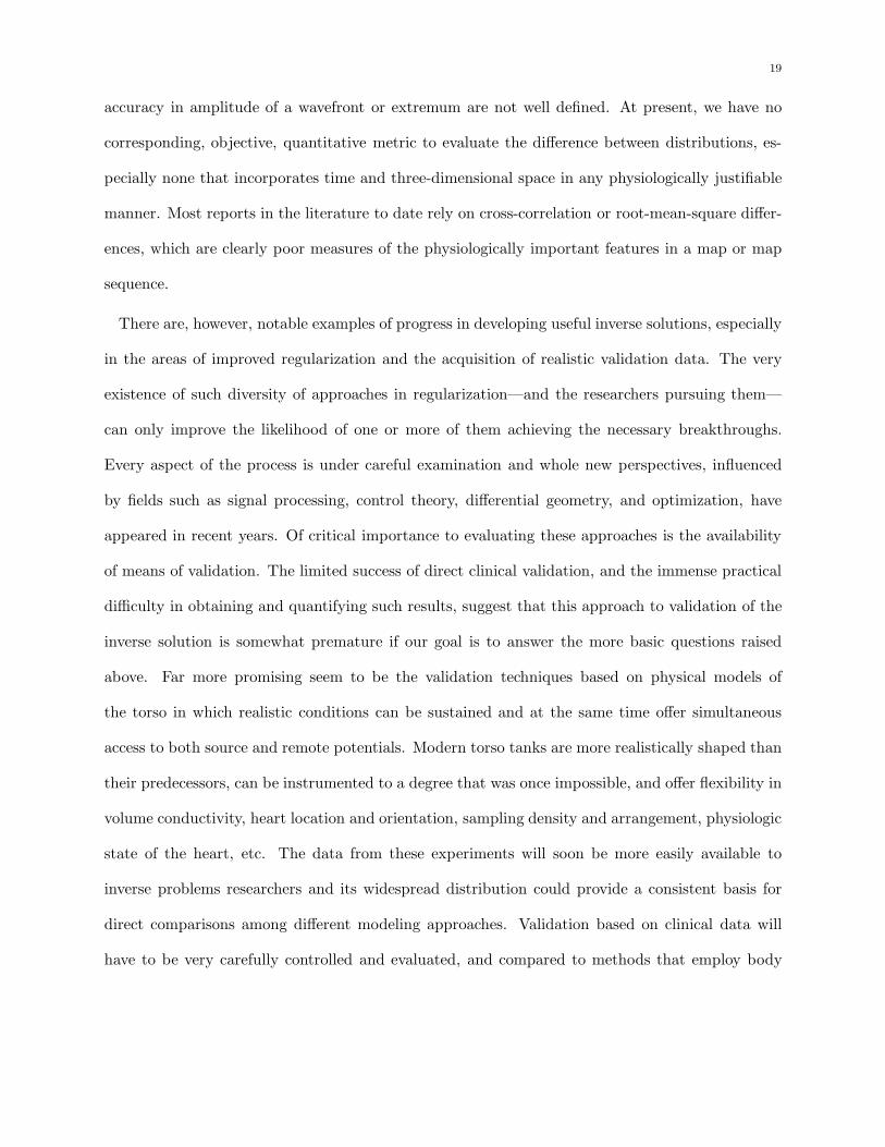
loon inflation. MacLeod, et al., computed epicardial potentials from patients during angioplasty

and compared locations of ST-segment elevations with the locations of the balloon catheter [93],

an example of which is shown in Fig. 3. This figure contains isopotential maps from corresponding

instants from two beats, one recorded before inflation of the angioplasty balloon (upper panel) and

the other during the latter phase of the inflation of the left circumflex artery (lower panel). The

epicardial maps were computed from the measured torso potentials using a realistic torso model,

a boundary element solution, and regularization with a single, Laplacian constraint [93]. During

inflation, anterior torso potentials become more negative than at rest while the posterior torso

shows a broad positive area suggestive of ischemia, but too diffuse for localization. The computed

epicardial potentials, on the other hand, indicate a very local area of positive potentials on the

postero-inferior aspect of the heart, suggestive of local acute ischemia. The estimated epicardial

ischemia zone lies just distal to the site of the angioplasty balloon, within the approximate perfusion

17

area supplied by the distal circumflex artery. While this validation result is encouraging, it is still

very qualitative in nature, and contains unexplained anomalies such as a second area of positive

potential in the atrial region, visible in the posterior view of the epicardium (lower right view in

the figure).

Another recent example of direct clinical application and validation is the use of an inverse so-

lution to predict sites of pre-excitation in Wolff-Parkinson-White patients based on body surface

potentials recorded before their ablation procedures [65, 94]. Inverse-computed epicardial maps from

the first 30 ms of the delta waves showed distinct minima that indicated earliest pre-excitation,

especially for sites on the free wall of the left ventricle. Shahidi, et al., performed detailed com-

parison of not only the site of pre-excitation, but also epicardial distributions recorded during

subsequent ablation surgery. They had limited success in predicting the measured potentials with

relative errors in the range of 100% and correlation coefficients from 0.22–0.34 [65]. They attributed

these discrepancies to errors in geometrical reconstruction of the epicardial surface and the sock

electrodes on that surface, as well as the effect of air exposure of the epicardial electrodes during

the open-chest measurements. They also found that errors paradoxically increased with improved

model resolution and the inclusion of inhomogeneities. The proposed reasons for this finding was

that more detail in the model increased the ill-conditioning of the forward solution matrix.

Please place Figure 3 here

Conclusions

The considerable progress achieved in the inverse problem of electrocardiography over the last

decade has provided grounds for optimism about the possibility of approaching significant clinically-

relevant applications in the next decade. However, there are a number of basic questions which

still remain. In addressing these questions, we feel it is important to seek solutions that emphasize

physiological rather than mathematical significance. This leads to twin requirements for useful

18

inverse solutions: accuracy, defined in a physiologically meaningful (and not just averaged and

mathematical) sense, and reliability, not only to measurement noise but also to geometric modeling

errors and other uncertainties which are inescapable in a practical application scenario. Studies

using analytically tractable models may still be relevant, but it seems more important to find

solutions to practical inverse problems that move the field towards wider acceptance and credibility.

From the discussion above we suggest the following three questions as critically important:

• What are the advantages and limitations of UDL or breakthrough-based methods compared

to potential methods? For example, under physiologically reasonable conditions, what useful

information, if any, can be reliably extracted from reconstructed potentials that is not present

in the activation-based models? How much less reliable are activation wavefronts reconstructed

from the potential-based solutions than those estimated from an activation-model formulation

such as UDL?

• What are the effects of approximations such as discretization error, spatial sampling density,

and the effects of inclusion/exclusion of various conductivity inhomogeneities? How do these

errors affect the accuracy and reliability of inverse solutions?

• What are the advantages and limitations of various regularization methods? What is the best

way to include a priori information? How can we decide which constraints are the most useful

to include? To what extent do the increased computational efforts of more recent methods

increase accuracy and reliability?

One basic question that affects our ability to answer these questions, using any of the formula-

tions we have discussed, is how to compare results quantitatively. How different is one isochrone

map or potential map sequence from another? How do we determine whether, and to what degree,

new solution methods are converging toward the correct solution or away from it? Experienced

electrophysiologists tend to use qualitative measures based on visual inspection to determine the

accuracy and validity of a map result. Even here tradeoffs between, say, accuracy in location and

19

accuracy in amplitude of a wavefront or extremum are not well defined. At present, we have no

corresponding, objective, quantitative metric to evaluate the difference between distributions, es-

pecially none that incorporates time and three-dimensional space in any physiologically justifiable

manner. Most reports in the literature to date rely on cross-correlation or root-mean-square differ-

ences, which are clearly poor measures of the physiologically important features in a map or map

sequence.

There are, however, notable examples of progress in developing useful inverse solutions, especially

in the areas of improved regularization and the acquisition of realistic validation data. The very

existence of such diversity of approaches in regularization—and the researchers pursuing them—

can only improve the likelihood of one or more of them achieving the necessary breakthroughs.

Every aspect of the process is under careful examination and whole new perspectives, influenced

by fields such as signal processing, control theory, differential geometry, and optimization, have

appeared in recent years. Of critical importance to evaluating these approaches is the availability

of means of validation. The limited success of direct clinical validation, and the immense practical

difficulty in obtaining and quantifying such results, suggest that this approach to validation of the

inverse solution is somewhat premature if our goal is to answer the more basic questions raised

above. Far more promising seem to be the validation techniques based on physical models of

the torso in which realistic conditions can be sustained and at the same time offer simultaneous

access to both source and remote potentials. Modern torso tanks are more realistically shaped than

their predecessors, can be instrumented to a degree that was once impossible, and offer flexibility in

volume conductivity, heart location and orientation, sampling density and arrangement, physiologic

state of the heart, etc. The data from these experiments will soon be more easily available to

inverse problems researchers and its widespread distribution could provide a consistent basis for

direct comparisons among different modeling approaches. Validation based on clinical data will

have to be very carefully controlled and evaluated, and compared to methods that employ body

20

surface map patterns directly [95, 96], to define limits of clinical utility.

The promise of the electrocardiographic inverse solution has been clear for a very long time;

the amount of effort that has been invested in solving the inverse problem is a tribute to its

desirability as well as its inherent difficulty. Existing solutions to the inverse problem do not yet

deserve consideration as realistic clinical tools, but recent progress has been remarkable. Through

synergistic efforts of modelers and experimentalists, further progress and eventual success seem

assured.

21

Authors’ bios

Robert S. MacLeod received both his B.Sc. (’79) in Engineering Physics and his Ph.D.(’90) in Physiology and Biophysics from Dalhousie University. His M.Sc. (’85) in ElectricalEngineering came from the Technische Universitat, Graz, Austria. He is an Assistant Professorin the Department of Internal Medicine (Div. of Cardiology) and Dept. of Bioengineering atthe University of Utah, and a member of the Nora Eccles Harrison Cardiovascular Research andTraining Institute. His research interests include computational electrocardiography (forwardand inverse problems), experimental investigation and clinical detection of cardiac ischemia andrepolarization abnormalities, and scientific computing and visualization.

Dana H. Brooks received the BSEE (’86), MSEE (’88), and Ph.D. (’91) degress in Electri-cal Engineering from Northeastern University in Boston, MA. He also earned a BA in English(’72) from Temple University. He is currently an assistant professor in the Electrical and Com-puter Engineering Department, Associate Director of the Center for Communications and Dig-ital Signal Processing, and PI of the Biomedical Signal Processing Lab, at Northeastern. Hispresent research interests include statistical and biomedical signal processing, applications ofmulti-resolution transforms, and tracking of small targets in infrared image sequences. He hasspecific interests in the application of advanced signal processing techniques to electrocardiog-raphy, including analysis of cardiac maps as well as the inverse problem of electrocardiography.

He also has ongoing projects in electromyography, phonocardiography, and decomposition of multi-unit nerve signalin lobsters.

22

References

[1] Messinger-Rapport, B. J. and Rudy, Y.: Regularization of the inverse problem in electrocar-

diography: A model study. Math Biosci 89:79–118, 1988.

[2] Rudy, Y. and Messinger-Rapport, B. J.: The inverse solution in electrocardiography: Solutions

in terms of epicardial potentials. CRC Crit Rev Biomed Eng 16:215–268, 1988.

[3] Gulrajani, R. M., Savard, P., and Roberge, F. A.: The inverse problem in electrocardiography:

Solutions in terms of equivalent sources. CRC Crit Rev Biomed Eng 16:171–214, 1988.

[4] Gulrajani, R. M.: Models of the electrical activity of the heart and the computer simulation

of the electrocardiogram. CRC Crit Rev Biomed Eng 16:1–66, 1988.

[5] Gulrajani, R. M., Roberge, F. A., and Mailloux, G. E.: The forward problem of electrocardio-

graphy. In: Macfarlane, P. W. and Lawrie, T. D. Veitch (Eds): Comprehensive Electrocardi-

ology. Pergamon Press, Oxford, England, pp 197–236, 1989.

[6] Gulrajani, R. M., Roberge, F. A., and Savard, P.: The inverse problem of electrocardiography.

In: Macfarlane, P. W. and Lawrie, T. D. Veitch (Eds): Comprehensive Electrocardiology.

Pergamon Press, Oxford, England, pp 237–288, 1989.

[7] Horacek, B.M.: The forward and inverse problem of electrocardiography. In: Ghista, D.N.

(Ed): 2nd Gauss Symposium: Medical Mathematics and Physics. Vieweg-Verlag, Wiesbaden,

1995.

[8] Greensite, F.: The mathematical basis for imaging cardiac electrical function. CRC Crit Rev

Biomed Eng 22:347–399, 1994.

[9] Rudy, Y: The electrocardiogram and its relationship to excitation of the heart. In: Spere-

lakis, N. (Ed): Physiology and Pathophysiology of the Heart. 3rd edition, Kluwer Academic

Publishers Group, chapter 11, pp 201–239, 1995.

[10] Barr, R. C. and Spach, M. S.: Inverse solutions directly in terms of potentials. In: Nelson, C. V.

and Geselowitz, D. B. (Eds): The Theoretical Basis of Electrocardiography. Clarendon Press,

23

Oxford, pp 294–304, 1976.

[11] de Bakker, J. M. T., Janse, M. J., van Capelle, J. J. L., and D., Durrer: Epicardial mapping

by simultaneous recording of epicardial electrograms during cardiac surgery for ventricular

aneurism. J Am Coll Cardiol 2:947–953, 1983.

[12] Downar, E., Parson, I. D., Mickleborough, L. L., Cameron, D. A., Yao, L. C., et al.: On-line

epicardial mapping of intraoperative ventricular arrhythmias: Initial clinical experience. J Am

Coll Cardiol 4:703–14, Oct. 1984.

[13] Bonneau, G., Tremblay, G., Savard, P., Guardo, R., Leblanc, A. R., et al.: An integrated

system for real-time cardiac activation mapping. IEEE Trans Biomed Eng BME-34:415–423,

1987.

[14] Derfus, D. L., Pilkington, T. C., and Ideker, R. E.: Calculating intracavitary potentials from

measured endocardial potentials. In: IEEE Engineering in Medicine and Biology Society 12th

Annual International Conference. IEEE Press, p 635, 1990.

[15] Khoury, D. S., Taccardi, B., Lux, R. L., Ershler, P. R., and Rudy, Y., et al.: Reconstruc-

tion of endocardial potentials and activation sequences from intracavity probe measurements.

Circulation 91:845–863, 1995.

[16] Cuppen, J. J. M. and van Oosterom, A.: Model studies with the inversely calculated isochrones

of ventricular depolarization. IEEE Trans Biomed Eng BME-31:652–659, 1984.

[17] Huiskamp, G. J. and van Oosterom, A.: The depolarization sequence of the human heart

surface computed from measured body surface potentials. IEEE Trans Biomed Eng BME-

35:1047–1059, 1989.

[18] Roberts, D. E., Hersh, L. T., and Scher, A. M.: Influence of cardiac fiber orientation on

wavefront voltage, conduction velocity, and tissue resistivity in the dog. Circ Res 44:701–712,

1979.

[19] Spach, M. S., Miller, W. T., Miller-Jones, E., Warren, R. B., and Barr, R. C., et al.: Ex-

24

tracellular potentials related to intracellular action potentials during impulse conduction in

anisotropic canine cardiac muscle. Circ Res 4:188–204, 1979.

[20] Taccardi, B., Macchi, E., Lux, R. L., Ershler, P. R., Spaggiari, S., et al.: Effect of myocardial

fiber direction on epicardial potentials. Circulation 90:3076–3090, 1994.

[21] Thivierge, M., Gulrajani, R.M., and Savard, P.: The effects of rotational myocardial anisotropy

in forward potential computations with equivalent heart dipoles. Annal Biomed Eng 1997 (in

press).

[22] Taccardi, B., Lux, R. L., MacLeod, R. S., and Ershler, P. R.: Anatomical stucture and

electrical activity of the heart. Acta Cardiologica 51(6):(in press), 1996.

[23] Lander, P. and Berbari, E.: Contouring of epicardial activation using spatial autocorrelation

estimates. In: IEEE Computers in Cardiology. IEEE Computer Society, pp 541–544, 1992.

[24] Bayley, R. H., Kalbfleisch, J. M., and Berry, P. M.: Changes in the body’s QRS surface

potentials produced by alterations in certain compartments of the nonhomogeneous conducting

model. Am. Heart J. 77, 1969.

[25] Rudy, Y. and Plonsey, R.: The eccentric spheres model as the basis for a study of the role of

geometry and inhomogeneities in electrocardiography. IEEE Trans Biomed Eng BME-26:392–

399, 1979.

[26] Rudy, Y. and Plonsey, R.: The effects of variations in conductivity and geometrical parameters

on the electrocardiogram, using an eccentric spheres model. Circ Res 44(1):104–111, 1979.

[27] Rudy, Y. and Plonsey, R.: A comparison of volume conductor and source geometry effects on

body surface and epicardial potentials. Circ Res 46:283–291, 1980.

[28] Barr, R. C., Ramsey, M., and Spach, M. S.: Relating epicardial to body surface potential

distributions by means of transfer coefficients based on geometry measurements. IEEE Trans

Biomed Eng BME-24:1–11, 1977.

[29] Barr, R. C. and Spach, M. S.: A comparison of measured epicardial potentials with epicardial

25

potentials computed from body surface measurements in the intact dog. Adv Cardiol 21:19–22,

1978.

[30] Franzone, P. Colli, Taccardi, B., and Viganotti, C.: An approach to inverse calculation of

epicardial potentials from body surface maps. Adv Cardiol 21:50–54, 1978.

[31] Franzone, P. Colli, Gassaniga, G., Guerri, L., Taccardi, B., and Viganotti, C., et al.: Accuracy

evaluation in direct and inverse electrocardiology. In: Macfarlane, P. W. (Ed): Progress in

Electrocardiography. Pitman Medical, pp 83–87, 1979.

[32] Yamashita, Y. and Takahashi, T.: Use of the finite element method to determine epicardial

from body surface potentials under a realistic torso model. IEEE Trans Biomed Eng BME-

31:611–621, 1984.

[33] van Oosterom, A.: Triangulating the human torso. Computer J 21:253–258, 1978.

[34] MacLeod, R. S., Johnson, C. R., and Ershler, P. R.: Construction of an inhomogeneous model

of the human torso for use in computational electrocardiography. In: IEEE Engineering in

Medicine and Biology Society 13th Annual International Conference. IEEE Press, pp 688–689,

1991.

[35] Johnson, C. R. and MacLeod, R. S.: Computer models for calculating transthoracic current

flow. In: IEEE Engineering in Medicine and Biology Society 13th Annual International Con-

ference. IEEE Press, pp 768–769, 1991.

[36] Johnson, C. R., MacLeod, R. S., and Ershler, P. R.: A computer model for the study of

electrical current flow in the human thorax. Computers in Biology and Medicine 22:305–323,

1992.

[37] Schmidt, J. A., Johnson, C. R., Eason, J. A., and MacLeod, R. S.: Applications of auto-

matic mesh generation and adaptive methods in computational medicine. In: Flaherty, J. and

Babuska, I. (Eds): Modeling, Mesh Generation, and Adaptive Methods for Partial Differential

Equations. Springer Verlag, pp 367–394, 1994.

26

[38] Klepfer, R. N., Johnson, C. R., and MacLeod, R. S.: The effects of inhomogeneities and

anisotropies on electrocardiographic fields: A three-dimensional finite elemental study. In:

IEEE Engineering in Medicine and Biology Society 17th Annual International Conference.

IEEE Press, pp 233–234, 1995.

[39] Akiyama, T., Richeson, J. F., Ingram, J. T., and Oravec, J.: Effects of varying the electrical

conductivity of the medium between the heart and the body surface on the epicardial and

precordial electrocardiogram in the pig. Card Res 12:697–702, 1978.

[40] Green, L. S., Taccardi, B., Ershler, P. R., and Lux, R. L.: Epicardial potential mapping:

Effects of conducting media on isopotential and isochrone distributions. Circulation 84:2513–

2521, 1991.

[41] MacLeod, R. S., Taccardi, B., and Lux, R. L.: The influence of torso inhomogeneities on

epicardial potentials. In: IEEE Computers in Cardiology. IEEE Computer Society, pp 793–

796, 1994.

[42] Pilkington, T. C., Morrow, M. N., and Stanley, P. C.: A comparison of finite element and

integral equation formulations for the calculation of electrocardiographic potentials - II. IEEE

Trans Biomed Eng BME-34:258–260, 1987.

[43] Meijs, J. W. H., Weier, O. W., Peters, M. J., and van Oosterom, A.: On the numerical accuracy

of the boundary element method. IEEE Trans Biomed Eng BME-36:1038–1049, 1989.

[44] MacLeod, R. S.: Percutaneous Transluminal Coronary Angioplasty as a Model of Cardiac

Ischemia: Clinical and Modelling Studies. PhD thesis, Dalhousie University, Halifax, N.S.,

Canada, 1990.

[45] Yu, F. Johnson, C. R.: An automatic adaptive refinement and derefinement method. In: Pro-

ceedings of the 14th IMACS World Congress. pp 1555–1557, 1944.

[46] Johnson, C. R. and MacLeod, R. S.: Nonuniform spatial mesh adaption using a posteriori

error estimates: applications to forward and inverse problems. Appl. Num. Anal. 14:311–326,

27

1994.

[47] Pullan, A.: A high-order coupled finite/boundary element torso model. IEEE Trans Biomed

Eng BME-43(3):292–298, 1996.

[48] Livnat, Y. and R., Johnson C.: The effects of adaptive refinement on ill-posed inverse problems.

In: Conference on Physiological Imaging, Spectroscopy, and Early Diagnostic Methods. SPIE,

1997 (submitted).

[49] Tikhonov, A. and Arsenin, V.: Solution of Ill-posed Problems. Winston, Washington, DC

1977.

[50] Groetsch, C. W.: The Theory of Tikhonov Regularization for Fredholm Equations of the First

Kind. Pitman, Boston 1984.

[51] Hansen, P. C.: Analysis of discrete ill-posed problems by means of the L-curve. SIAM Review

34(4):561–580, 1992.

[52] Hansen, P.C: Rank-deficient and discrete ill-posed problems. PhD thesis, Technical University

of Denmark, 1996.

[53] Brooks, D. H., Nikias, C. L, and Siegel, J. H.: An inverse solution in electrocardiography in

the frequency domain. In: IEEE Engineering in Medicine and Biology Society 10th Annual

International Conference. pp 970–971, 1988.

[54] Johnson, C. R. and MacLeod, R. S.: Local regularization and adaptive methods for the inverse

Laplace problem. In: Ghista, D. N. (Ed): 2nd Gauss Symposium: Medical Mathematics and

Physics. Vieweg-Verlag, Wiesbaden, 1996. (in press).

[55] Horacek, B.M., Penny, C.J., and Clements, J.C.: Inverse solutions in terms of single- and

double-layer. Annal Biomed Eng 24(suppl. 1):58, 1996.

[56] Throne, R. D., Olson, L. G., Hrabik, T. J., and Windle, J. R.: Generalized eigensystem

techniques for the inverse problem of electrocardiography applied to a realistic heart-torso

geometry. IEEE Trans Biomed Eng (in press), 1997.

28

[57] Khoury, D.: Use of current density in the regularization of the inverse problem of electrocar-

diography. In: IEEE Engineering in Medicine and Biology Society 16th Annual International

Conference. IEEE Press, pp 133–134, 1994.

[58] Oster, H. S. and Rudy, Y.: The use of temporal information in the regularization of the inverse

problem of electrocardiography. IEEE Trans Biomed Eng BME-39(1):65–75, 1992.

[59] Brooks, D. H., Maratos, G. M., Ahmad, G., and MacLeod, R. S.: The augmented inverse prob-

lem of electrocardiography: combined time and space regularization.. In: IEEE Engineering in

Medicine and Biology Society 15th Annual International Conference. IEEE Press, pp 773–774,

1993.

[60] Brooks, D. H., Ahmad, G., and MacLeod, R. S.: Multiply constrained inverse electrocardiology:

Combining temporal, multiple spatial, and and iterative regularization. In: IEEE Engineering

in Medicine and Biology Society 16th Annual International Conference. IEEE Computer

Society, pp 137–138, 1994.

[61] Brooks, D. H., Ahmad, G. F., MacLeod, R. S., and Maratos, G. M.: Inverse electrocardiogra-

phy by simultaneous imposition of multiple constraints. IEEE Trans Biomed Eng (submitted),

1997.

[62] El-Jakl, J., Champagnat, F., and Goussard, Y.: Time-space regularization of the inverse prob-

lem of electrocardiography. In: IEEE Engineering in Medicine and Biology Society 17th Annual

International Conference. 1995.

[63] Greensite, F.: Two mechanisms for electrocardiographic deconvolution. In: IEEE Engineering

in Medicine and Biology Society 18th Annual International Conference. 1996.

[64] Brooks, D.H. and Ahmad, R.S, G.F.and MacLeod: Multiply constrained inverse electrocar-

diography: Combining temporal, multiple spatial, and iterative regularization. In: IEEE En-

gineering in Medicine and Biology Society 16th Annual International Conference. IEEE Press,

1994.

29

[65] Shahidi, A. V., Savard, P., and Nadeau, R.: Forward and inverse problems of electrocardio-

graphy: Modeling and recovery of epicardial potentials in humans. IEEE Trans Biomed Eng

BME-41(3):249–256, 1994.

[66] Ahmad, G. F., Brooks, D. H., Jacobson, C. A., and MacLeod, R. S.: Constraint evaluation in

inverse electrocardiography using convex optimization. In: IEEE Engineering in Medicine and

Biology Society 17th Annual International Conference. IEEE Press, pp 209–210, 1995.

[67] Ahmad, G.F, Brooks, D.H., and MacLeod, R.S.: An admissible solution approach to inverse

electrocardiography. Annal Biomed Eng (submitted), 1996.

[68] Greensite, F.: Demonstration of “discontinuities” in the true derivative of body surface po-

tential, and their prospective role in noninvasive imaging of the ventricular surface activation

map. IEEE Trans Biomed Eng BME-40(12):1210–1218, 1993.

[69] Greensite, F.: Well-Posed formulation of the inverse problem of electrocardiography. Annal

Biomed Eng 22:172–183, 1994.

[70] Greensite, F, Qian, Y-J, and Huiskamp, G.: Myocardial activation imaging: a new theorem

and its implications. In: IEEE Engineering in Medicine and Biology Society 17th Annual

International Conference. 1995.

[71] Iakovidis, I. and Gulrajani, R.M.: Improving Tikhonov regularization with linearly constrained

optimization: Application to the inverse epicardial potential solution. Mathematical Bio-

sciences 112:55–80, 1992.

[72] Messinger-Raport, B. J. and Rudy, Y.: Noninvasive recovery of epicardial potentials in a

realistic heart-torso geometry. Circ Res 66, 4:1023–1039, 1990.

[73] Oster, H.S. and Rudy, Y.: Regional regularization of the electrocardiographic inverse problem:

a model study using spherical geometry. IEEE Trans Biomed Eng 1997 (in press).

[74] Pieper, C. F. and Pacifico, A.: The epicardial field potential in dog: Implications for recording

site density during epicardial mapping. PACE 16:1263–1274, June 1993.

30

[75] Arisi, G., Macchi, E., Corradi, C., Lux, R. L., and Taccardi, B., et al.: Epicardial excita-

tion during ventricular pacing: Relative independence of breakthrough sites from excitation

sequence in canine right ventricle. Circ Res 71(4):840–849, 1992.

[76] H., Bayley R. and M., Berry P.: The electrical field produced by the eccentric current dipole

in the nonhomogeneous conductor. Am. Heart J. 63, 1962.

[77] Iakovidis, I. and Gulrajani, R. M.: Regularization of the inverse epicardial solution using

linearly constrained optimization. In: IEEE Engineering in Medicine and Biology Society 13th

Annual International Conference. IEEE Press, pp 698–699, 1991.

[78] Throne, R. and Olsen, L.: A generalized eigensystem aproach to the inverse problem of

electrocardiography. IEEE Trans Biomed Eng BME-41:592–600, 1994.

[79] Throne, R. and Olsen, L.: The effect of errors in assumed conductivities and geometry on

numerical solutions to the inverse problem of electrocardiography. IEEE Trans Biomed Eng

BME-42, 1995.

[80] Barr, R. C., Pilkington, T. C., Boineau, J. P., and Spach, M. S.: Determining surface potentials

from current dipoles, with application to electrocardiography. IEEE Trans Biomed Eng BME-

13:88–92, 1966.

[81] Durrer, D., van Dam, R. T., Freud, G. E., Janse, M. J., Meijler, F. L., et al.: Total excitation

of the isolated human heart. Circulation 41:899–912, 1970.

[82] Horacek, B. M., de Boer, R. G., Leon, J. L., and Montague, T. J.: Human epicardial potential

distributions computed from body-surface-available data. In: Yamada, K., Harumi, K., and

Musha, T. (Eds): Advances in Body Surface Potential Mapping. University of Nagoya Press,

Nagoya, Japan, pp 47–54, 1983.

[83] Burger, H. C. and van Milaan, J. B.: Heart-vector and leads. Part II. Br Heart J 9:154–60,

1947.

[84] Nagata, Y.: The influence of the inhomogeneities of electrical conductance within the torso

31

on the electrocardiogram as evaluated from the view point of the transfer impedance vector.

Jap Heart J 11(5):489–505, 1970.

[85] DeAmbroggi, L. and Taccardi, B.: Current and potential fields generated by two dipoles. Circ

Res 27:910–911, 1970.

[86] Johnson, C. R.: The Generalized Inverse Problem in Electrocardiography: Theoretical, Com-

putational and Experimental Results. PhD thesis, University of Utah, Salt Lake City, Utah,

1989.

[87] Stanley, P. C., Pilkington, T. C., and Morrow, M. N.: The effects of thoracic inhomogeneities

on the relationship between epicardial and torso potentials. IEEE Trans Biomed Eng BME-

33:273–284, 1986.

[88] Soucy, B., Gulrajani, R. M., and Cardinal, R.: Inverse epicardial potential solutions with an

isolated heart preparation. In: IEEE Engineering in Medicine and Biology Society 11th Annual

International Conference. IEEE Press, pp 193–194, 1989.

[89] Oster, H. S., Taccardi, B., Lux, R. L., Ershler, P. R., and Rudy, Y., et al.: Noninvasive electro-

cardiographic imaging: Reconstruction of epicardial potentials, electrograms, and isochrones

and localization of single and multiple electrocardiac events. Circulation (in press), 1997.

[90] MacLeod, R. S., Taccardi, B., and Lux, R. L.: Electrocardiographic mapping in a realistic

torso tank preparation. In: IEEE Engineering in Medicine and Biology Society 17th Annual

International Conference. IEEE Press, pp 245–246, 1995.

[91] MacLeod, R. S., Taccardi, B., and Lux, R. L.: Mapping of cardiac ischemia in a realistic

torso tank preparation. In: Building Bridges: International Congress on Electrocardiology

International Meeting. pp 76–77, 1995.

[92] Gruntzig, A. R., Senning, A., and Siegenthaler, W. E.: Nonoperative dilatation of coronary

artery stenosis. New Eng J Med 301:61–68, 1979.

[93] MacLeod, R. S., Miller, R. M., Gardner, M. J., and Horacek, B. M.: Application of an elec-

32

trocardiographic inverse solution to localize myocardial ischemia during percutaneous translu-

minal coronary angioplasty. J Cardiovasc Electrophysiol 6:2–18, 1995.

[94] Penney, C. J., Clements, J. C., Gardner, M. J., Sterns, L., and Horacek, B. M., et al.: The

inverse problem of electrocardiography: application to localization of Wolff-Parkinson-White

pre-excitation sites. In: IEEE Engineering in Medicine and Biology Society 17th Annual In-

ternational Conference. IEEE Press, pp 215–216, 1995.

[95] Simelius, K., Jokiniemi, T., Nenonen, J., Tierala, I., Toivonen, L., et al.: Arrythmia localiza-

tion using body surface potential mapping during catheterization. In: IEEE Engineering in

Medicine and Biology Society 18th Annual International Conference. 1996.

[96] Potse, M., Linnenbank, A.C., SippensGroenewegen, A., and Grimbergen, C.A.: Continuous

localization of ectopic left ventricular activation sites by means of a two-dimensional repre-

sentation of body surface ARS integral maps. In: IEEE Engineering in Medicine and Biology

Society 18th Annual International Conference. 1996.

33

+-

-

+-

A

B

C

--++

-++

Fig. 1. Inverse problem formulations. Panel A shows the potential based formulation for epicardial potentials(shaded area) and measurement electrodes on the body surface. Panel B shows a potential basedformulation where endocardial potentials are the source and measurement electrodes are mounted in acatheter probe. Panel C represents the UDL formulation, in which the activation wavefront serves asthe source.

34

10 20 30 40 50 60

−2000

0

2000

10 20 30 40 50 60

−2000

0

2000

10 20 30 40 50 60

−2000

0

2000

10 20 30 40 50 60

−2000

0

2000

10 20 30 40 50 60

−2000

0

2000

10 20 30 40 50 60

−2000

0

2000

10 20 30 40 50 60

−2000

0

2000

10 20 30 40 50 60

−2000

0

2000

Fig. 2. Comparison of spatial to joint spatial and temporal regularization: Four epicardial electrograms areshown for 60 ms during QRS. The first and third rows contain results from spatial regularization, theother rows joint time/space regularization. In each panel the solid line is the original electrogram andthe other lines correspond to various regularization parameters.

35

Pre PTCA

Post PTCA

Anterior View Posterior View

Fig. 3. Inverse solution validation using maps from angioplasty patients. The upper panel contains measuredbody-surface and inverse-computed epicardial potentials from a single instant (marked by the verticalline on the ECG) during a beat recorded before inflation of the angioplasty balloon. In the lower panel,corresponding maps from the peak phase of the angioplasty inflation show the effects of acute occlusionof the left circumflex coronary artery (balloon location marked by arrow). The left-hand column showsthe anterior views of both torso and epicardium, while the right-hand column shows the posterior views.Circles in the anterior torso views indicate the locations of standard leads V1 −−V6. Color representselectric potential in a scale the goes from blue (most negative) through green, yellow, and red (mostpositive).