Embed Size (px)
Citation preview

Lehigh UniversityLehigh Preserve
Theses and Dissertations
2013
Recent glacier surface snowpack melt in NovayaZemlya and Severnaya Zemlya derived from activeand passive microwave remote sensing dataMeng ZhaoLehigh University
Follow this and additional works at: http://preserve.lehigh.edu/etd
Part of the Physical Sciences and Mathematics Commons
This Thesis is brought to you for free and open access by Lehigh Preserve. It has been accepted for inclusion in Theses and Dissertations by anauthorized administrator of Lehigh Preserve. For more information, please contact [email protected].
Recommended CitationZhao, Meng, "Recent glacier surface snowpack melt in Novaya Zemlya and Severnaya Zemlya derived from active and passivemicrowave remote sensing data" (2013). Theses and Dissertations. Paper 1697.

Recent glacier surface snowpack melt in Novaya Zemlya and Severnaya Zemlya derived
from active and passive microwave remote sensing data
by
Meng Zhao
A Thesis
Presented to the Graduate and Research Committee
of Lehigh University
in Candidacy for the Degree of
Master of Science
in
Earth and Environmental Sciences Department
Lehigh University
April 26, 2013

ii
© 2013 Copyright
Meng Zhao

iii
Thesis is accepted and approved in partial fulfillment of the requirements for the Master
of Science in Earth and Environmental Sciences.
RECENT GLACIER SURFACE SNOWPACK MELT IN NOVAYA ZEMLYA AND
SEVERNAYA ZEMLYA DERIVED FROM ACTIVE AND PASSIVE MICROWAVE
REMOTE SENSING DATA
MENG ZHAO
Date Approved
Dr. Joan Ramage
Thesis Director
Dr. Benjamin Felzer
Committee Member
Dr. Dork Sahagian
Committee Member
Dr. Frank Pazzaglia
Department Chair

iv
ACKNOWLEDGEMENTS
I would like to thank my advisor, Joan Ramage, first for providing me with the
opportunity to pursue an advanced degree in Earth and Environmental Sciences at Lehigh
University, and secondly for her warmhearted help and support on both my study and
new life in the United States. I also want to thank my committee members, Benjamin
Felzer and Dork Sahagian, for their support and useful suggestions. In addition, I want to
thank my fellow graduate student Kathryn Semmens for her help and suggestions.
Thanks to Thomas Opel and Friedrich Obleitner for sharing automatic weather
station data. Also thanks to Microwave Earth Remote Sensing Laboratory at Brigham
Young University and the National Snow and Ice Data Center for providing microwave
remote sensing data. I also appreciate the glacier outline data provided by the Global
Land Ice Measurements from Space and reanalysis data provided by National Oceanic
and Atmospheric Administration. This research is partially funded by Lehigh University
and NASA grant #NNX11AR14G to Joan Ramage.
Special thanks to my parents, Yongfu Zhao and Yulan Li. Without their
tremendous financial and emotional support, it would take much more time and effort for
me to accomplish the present work. Thank you very much!

v
TABLE OF CONTENTS
LIST OF TABLES ............................................................................................................ vii
LIST OF FIGURES ......................................................................................................... viii
ABSTRACT ........................................................................................................................ 1
INTRODUCTION .............................................................................................................. 3
DATA ............................................................................................................................... 10
Glacier Outline .............................................................................................................. 10
In-situ Temperature Data ............................................................................................... 10
Microwave Remote Sensing Data ................................................................................. 13
Passive Microwave ..................................................................................................... 15
Active Microwave ...................................................................................................... 18
Reanalysis Air Temperature .......................................................................................... 21
Regional Sea Ice Extent ................................................................................................. 21
METHODS ....................................................................................................................... 22
Passive Microwave ........................................................................................................ 22
NSIDC SSM/I and AMSR-E melt signature literature review .................................. 22
MERSL-BYU SSM/I melt signature algorithm ......................................................... 24
MERSL-BYU AMSR-E melt signature algorithm .................................................... 36
Active Microwave ......................................................................................................... 38
MERSL-BYU QSCAT melt signature algorithm ...................................................... 38
MERSL-BYU ERS-1/2 melt signature algorithm ...................................................... 41
MERSL-BYU ASCAT melt signature algorithm ...................................................... 42
RESULTS ......................................................................................................................... 43
Sensor Time Series and In-situ Temperature Intercomparisons .................................... 43
MERSL-BYU SSM/I, ERS and in-situ temperature data .......................................... 43
MERSL-BYU AMSR-E, QSCAT and ASCAT ......................................................... 45
Cross-validations of MOD and TMD among Sensors ................................................... 47
MOD and TMD Trend ................................................................................................... 57
Relationships with Local Air Temperature ................................................................... 59
Relationships with Local Sea Ice Extent ....................................................................... 61
vi
DISCUSSION ................................................................................................................... 65
Mass Balance ................................................................................................................. 65
Paleo Perspective ........................................................................................................... 66
Limitations and Future Work ........................................................................................ 67
CONCLUSIONS............................................................................................................... 72
REFERENCES ................................................................................................................. 74
APPENDIX A: SSM/I MOD maps from 1995 to 2007 .................................................... 81
APPENDIX B: AMSR-E MOD maps from 2003 to 2011 ............................................... 86
APPENDIX C: ERS-1/2 MOD maps from 1992 to 2000 ................................................ 89
APPENDIX D: QSCAT MOD maps from 2000 to 2009 ................................................. 92
APPENDIX E: ASCAT MOD maps from 2009 to 2012 ................................................. 96
APPENDIX F: SSM/I TMD maps from 1995 to 2007 ..................................................... 98
APPENDIX G: AMSR-E TMD maps from 2003 to 2011 ............................................. 103
APPENDIX H: QSCAT TMD maps from 2000 to 2009 ............................................... 106
Curriculum Vitae ............................................................................................................ 110

vii
LIST OF TABLES
Table 1. Passive microwave data summary……………………………………………...17
Table 2. Active scatterometer data summary…………………………………………….20
Table 3. Pearson Coefficients of NSIDC and MERSL-BYU SSM/I data ........................28
Table 4. Melt onset, refreeze date and total melt days summary………………………...33
Table 5. A subset comparison between SSM/I Tb and air temperature……….....………34
Table 6. MOD and TMD retrieved from slice- and egg-based QSCAT data...………….40

viii
LIST OF FIGURES
Figure 1. Location of study area in the Russian High Arctic …………………………......7
Figure 2. Near-surface wind maps.......................................................................................8
Figure 3. Annual average near-surface air temperature anomalies...……………………...9
Figure 4. Pixel grid comparisons………………………………………………………...12
Figure 5. Satellite timeline.………………………….…………………………………...14
Figure 6. Tb distribution of MERSL-BYU SSM/I…………………...…………………..27
Figure 7. Tb histograms of NSIDC and MERSL-BYU SSM/I ………………………….29
Figure 8. Tb time series comparison between NSIDC and MERSL-BYU SSM/I.………32
Figure 9. An illustration of early melt event……………………………………………..35
Figure 10. Tb histograms of MERSL-BYU AMSR-E………………………………...…37
Figure 11. Microwave time series and in-situ temperature comparison..................….....44
Figure 12. AMSR-E, QSCAT and ASCAT time series comparison….…………….......46
Figure 13. Frequency distribution of MOD differences among sensors……………...….49
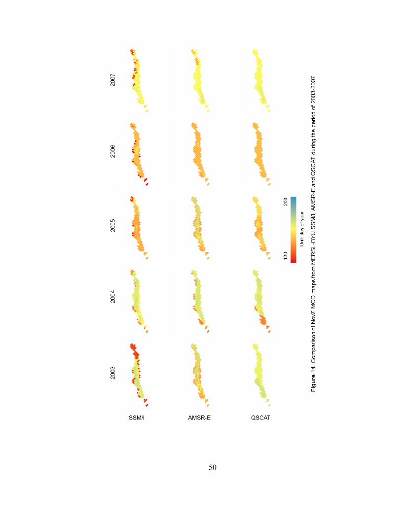
Figure 14. Comparison of NovZ MOD maps………………………………………........50
Figure 15. Comparison of SevZ MOD maps……………………………………..…..….51
Figure 16. Frequency distributions of TMD differences among sensors………….……..54
Figure 17. Comparison of NovZ TMD maps…………………………….………………55
Figure 18. Comparison of SevZ TMD maps…………………………………………….56
Figure 19. Decadal variations in annual MOD and TMD……………………………….58
Figure 20. Snowmelt relation with local reanalysis temperature………………………..60
Figure 21. TMD relation with regional sea ice extent…………………………………...63

ix
Figure 22. 2010 summer temperature anomaly compared to 1951-2000 mean……...….64
Figure 23. Satellite observation comparison at different local time of day……………...71

1
ABSTRACT
The warming rate in the Russian High Arctic (RHA) (36~158˚E, 73~82˚N) is
outpacing the pan-Arctic average, and its effect on the small glaciers across this region
needs further examination. The temporal variation and spatial distribution of surface melt
onset date (MOD) and total melt days (TMD) throughout the Novaya Zemlya (NovZ) and
Severnaya Zemlya (SevZ) archipelagoes serve as good indicators of ice mass ablation
and glacier response to regional climate change in the RHA. However, due to the harsh
environment, long-term glaciological observations are limited, necessitating the
application of remotely sensed data to study the surface melt dynamics. The high
sensitivity to liquid water and the ability to work without solar illumination and penetrate
non-precipitating clouds make microwave remote sensing an ideal tool to detect melt in
this region. This work extracts resolution-enhanced passive and active microwave data
from different periods and retrieves a decadal melt record for NovZ and SevZ. The high
correlation among passive and active data sets instills confidence in the results. The mean
MOD is June 20th
on SevZ and June 10th
on NovZ during the period of 1992-2012. The
average TMDs are 47 and 67 days on SevZ and NovZ from 1995 to 2011, respectively.
NovZ had large interannual variability in the MOD, but its TMD generally increased.
SevZ MOD is found to be positively correlated to local June reanalysis air temperature at
850hPa geopotential height and occurs significantly earlier (~0.73 days/year, p-value <
0.01) from 1992 to 2011. SevZ also experienced a longer TMD trend (~0.75 days/year, p-
value < 0.05) from 1995 to 2011. Annual mean TMD on both islands are positively

2
correlated with regional summer mean reanalysis air temperature and negatively
correlated to local sea ice extent. These strong correlations might suggest that the Russian
High Arctic glaciers are vulnerable to the continuously diminishing sea ice extent, the
associated air temperature increase and amplifying positive ice-albedo feedback, which
are all projected to continue into the future.

3
INTRODUCTION
Large Greenland and Antarctic ice sheets are known to be thinning at a fast rate in
response to increasing atmospheric warming and ocean temperature anomalies (e.g.,
IPCC, 2001; 2007; Nick et al., 2009; Velicogna, 2009), but the response of many smaller
glaciated regions need further examination (e.g., Smith et al., 2003; Moholdt et al., 2010;
Gardner et al., 2011). The heavily glaciated Novaya Zemlya (NovZ) and Severnaya
Zemlya (SevZ) archipelagoes in the Russian High Arctic (RHA) are among those
regions, which span a wide range of longitude and encompass more than 40,000 km2
glaciated areas combined (Fig. 1) (Bassford et al., 2006; Moholdt et al., 2012). The RHA
is influenced by westerlies, which are decreasing to the north. NovZ is in the zone of
northerly flow while SevZ is in the zone of southerly flow in the means during the period
of 1995-2011 (Fig. 2). The climate is mild and humid in the southwest NovZ and
gradually becomes dryer and colder northeast into SevZ (Kotlyako et al., 2010). The
annual mean air temperature ranges from -5˚C to -15˚C across this region with a July
mean air temperature slightly above 0˚C in SevZ and the northern tip of NovZ. NovZ is
in the path of the warm North Atlantic Drift current and the prevailing westerlies could
promote warm air advection, bringing moist westerly air masses from the Norwegian Sea
and resulting in a larger than SevZ precipitation and an annual July mean temperature of
6.5˚C (Zeeberg and Forman, 2001; Kotlyako et al., 2010; Moholdt et al., 2012). The
higher precipitation produces large areas of glaciation along the west coast of NovZ,
whose equilibrium line lies about 200 m lower than the west coast of SevZ (Kotlyako et
al., 2010).

4
In recent decades, pan-Arctic average air temperature has increased at a rate that
is twice the global average (Screen and Simmonds, 2010) and the RHA has experienced a
mean temperature increase of 1˚C to 3˚C with an even higher magnitude up to 5˚C for
winter seasons since the mid-1950s (Weller et al., 2005), outpacing many other Arctic
regions (Fig.3). This significant global and regional warming increases the vulnerability
of the small and low-elevation glaciers in SevZ and NovZ to mass loss, potentially
contributing a disproportionate amount of fresh water into the ocean (Moholdt et al.,
2012). Furthermore, rapidly diminishing summer sea ice extent is enhancing the warming
trend as a result of the strong positive ice-albedo feedback and changing ocean-
atmosphere heat flux transfer mechanism in Arctic (Jacob et al., 2012).
Snowpack melting plays an important role in the mass balance of the icecaps in
NovZ and SevZ (Dowdeswell and Hagen, 2004). Surface melting and refreezing
significantly change snowpack crystal size, morphology and emissivity, leading to
variations in the glacier surface energy balance by lowering albedo, which enhances the
absorption of solar radiation and amplifies the positive snow-albedo feedback (Mätzler,
1994). Surface melt water also drains into glacier bed, lubricating the ice-bedrock
interface and transferring latent heat to ice bottom, further increasing glacier flow
dynamics and calving (Zwally et al., 2002; Thomas et al., 2003; van den Broeke, 2005).
Melt onset date and total melt days are strongly correlated with glacier flow acceleration
and deceleration (Zwally et al., 2002). They are also good proxies in quantifying
snowmelt intensity (e.g., Smith et al., 2003; Trusel et al. 2012) as well as ice ablation
(Mote, 2003) and their long-term variations are important reflectors of glacier response to
regional climate variability (Tedesco et al., 2009). Therefore, monitoring the temporal

5
variation and spatial distribution of melt onset date (MOD) and total number of melt days
(TMD) in NovZ and SevZ significantly contributes to the understanding of large-scale
dynamics of ice masses throughout the RHA and couplings with regional and global
climate. However, due to the harsh environment, long term records of glaciological
observations are limited, necessitating the application of remotely sensed data to study
the surface melt dynamics on NovZ and SevZ.
The RHA is severely cloud-covered and lacking solar illumination for many days
each year, which substantially impact the continuous acquisition of useful satellite
imageries (Marshall et al., 1994). The high sensitivity to liquid water and independence
of cloud contamination as well as the ability to work without solar illumination makes
microwave remote sensing an ideal tool to detect melt in this environment. In this study,
decadal MOD and TMD time series, as well as spatial melt maps, are concatenated from
multiple passive and active microwave datasets after inter-calibration and used to answer
three scientific questions: 1) how did MOD and TMD vary spatially and temporally in the
past decades? 2) how did the surface melting respond to regional temperature change? 3)
is the glacier snow melt related to regional sea ice extent variations?
The “DATA” section introduces the passive and active microwave data, glacier
outlines, in-situ temperature record, and regional sea ice extent as well as reanalysis
temperature data. The “METHODS” section briefly reviews melt detection methods in
literature and develops retrieval algorithms for the microwave data employed by this
work. The “RESULTS” section cross-validates and inter-calibrates melt detection among
passive and active sensors, and presents answers to the above three scientific questions.
The “DISCUSSION” section puts the results in a mass balance and paleo perspective and

6
discusses limitations and future works. Finally, the “CONLUSION” section summarizes
findings and implications.

7
Figure 1. Location of study area in the Russian High Arctic under polar stereographic
projection. The relief is from ETOPO1 Global Relief Model (Amante and Eakins, 2009)
and the glacier extent is from Global Land Ice Measurements from Space (GLIMS)
(Raup et al., 2007), shown in a speckled pattern. The red box in the upper left panel
shows the global location of the Novaya Zemlya and Severnaya Zemlya in the high
Arctic. Shaded blue and red regions are Arctic Ocean and Kara and Barents Seas,
respectively, whose sea ice extents are correlated with snowpack melt on Severnaya
Zemlya and Novaya Zemlya. An automatic weather station (indicated as a green dot) was
maintained during an ice core drilling campaign on Akademii Nauk ice cap in Severnaya
Zemlya at 80˚31ʹN, 94˚49ʹE (Opel et al., 2009).

8
(a)
(b)
Figure 2. Annual average 850hPa geopotential height reanalysis wind maps of the
Russian High Arctic during 1995-2011. (a) is the zonal. (b) is meridional wind. Unit:
meter/second. (Figure courtesy: National Oceanic and Atmospheric Administration
(NOAA) Earth System Research (ESRL), available at:
http://www.esrl.noaa.gov/psd/data/histdata/)

9
Figure 3. Annual average near-surface air temperature anomalies for the first decade of
the 21st century (2001-11) relative to the baseline period of 1971-2000. The Russian High
Arctic is red-circled and its temperature increase is outpacing many other Arctic regions.
Unit: ˚C. (Figure courtesy: NOAA ESRL, available at:
http://www.esrl.noaa.gov/psd/data/histdata/)
10
DATA
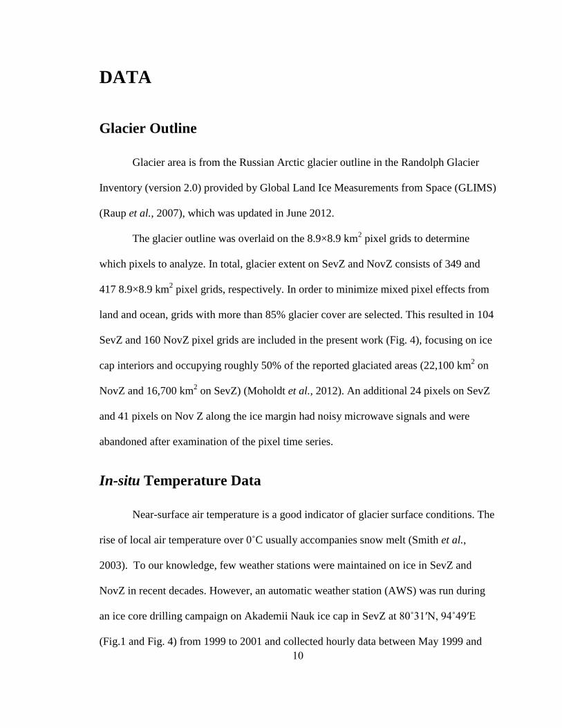
Glacier Outline
Glacier area is from the Russian Arctic glacier outline in the Randolph Glacier
Inventory (version 2.0) provided by Global Land Ice Measurements from Space (GLIMS)
(Raup et al., 2007), which was updated in June 2012.
The glacier outline was overlaid on the 8.9×8.9 km2 pixel grids to determine
which pixels to analyze. In total, glacier extent on SevZ and NovZ consists of 349 and
417 8.9×8.9 km2 pixel grids, respectively. In order to minimize mixed pixel effects from
land and ocean, grids with more than 85% glacier cover are selected. This resulted in 104
SevZ and 160 NovZ pixel grids are included in the present work (Fig. 4), focusing on ice
cap interiors and occupying roughly 50% of the reported glaciated areas (22,100 km2 on
NovZ and 16,700 km2 on SevZ) (Moholdt et al., 2012). An additional 24 pixels on SevZ
and 41 pixels on Nov Z along the ice margin had noisy microwave signals and were
abandoned after examination of the pixel time series.
In-situ Temperature Data
Near-surface air temperature is a good indicator of glacier surface conditions. The
rise of local air temperature over 0˚C usually accompanies snow melt (Smith et al.,
2003). To our knowledge, few weather stations were maintained on ice in SevZ and
NovZ in recent decades. However, an automatic weather station (AWS) was run during
an ice core drilling campaign on Akademii Nauk ice cap in SevZ at 80˚31ʹN, 94˚49ʹE
(Fig.1 and Fig. 4) from 1999 to 2001 and collected hourly data between May 1999 and

11
May 2000 with data gaps in February and April 2000 due to power breakdowns (Opel et
al., 2009).
Theoretically, the melting temperature of snowpack is determined from glacier
surface energy balance; however, the AWS data we have do not have necessary
measurements to solve energy balance equations. Therefore, present work assumes that
melting occurs when daily maximum temperature exceeds 0˚C following recent studies
(e.g., Tedesco et al., 2009; Trusel et al., 2012).

12
Figure 4. Pixel grid comparisons under polar stereographic projection. Black grids are
8.9×8.9 km2 and red grids are 4.45×4.45 km
2. Green grids are 25×25 km
2 grids. Purple
pixels are used to compare grid differences in the “METHODS” section. Blue
background is glacier extent from Global Land Ice Measurements from Space (Raup et
al., 2007). The automatic weather station (black dot) was maintained on Akademii Nauk
ice cap on Severnaya Zemlya. Note that the two archipelagoes are not in the same
projection.
Akademii
Nauk ice cap
Novaya
Zemlya
Severnaya
Zemlya

13
Microwave Remote Sensing Data
Microwave remote sensing data have been widely applied in snow mapping
because of their high sensitivity to liquid water in the snowpack, independence from solar
illumination, and lack of cloud contamination (Ashcraft and Long, 2006). There are two
major types of microwave remote sensing sensors: passive and active. Active sensors
transmit microwave energy to the earth’s surface and measure the reflected energy as
backscatter coefficient (σ0, unit: dB), which is a function of surface roughness, wetness,
land type, polarization, frequency, topography and sensor configurations (Hinse et al.,
1988). Instead of sending energy, passive microwave sensors directly collect earth
surface microwave self-emission as brightness temperature (Tb, unit: K), which is
approximated as a product of surface emissivity and physical temperature. Wet snow has
a much higher microwave emissivity than dry snow, which results in an abrupt and
distinct increase in a Tb time series when surface snow changes from a dry, frozen state to
a wet, melting state (Stiles and Ulaby, 1980). Conversely, the presence of liquid water
greatly reduces snowpack volume scattering and increases microwave absorption, leading
to a sharp decrease in active radar σ0 (Stiles and Ulaby, 1980). Microwave sensors
employed in the present work collectively covered a decadal period spanning from 1992
to 2012 (Fig. 5).

14
Figure 5. Satellite timeline. European Remote-Sensing (ERS) satellite data covered
1992-2000; QuikScat (QSCAT) data covered 2000-2009; Advanced Scatterometer
(ASCAT) covered 2000-2012; Special Sensor Microwave Imager (SSM/I) data covered
1995-2007; Advanced Microwave Scanning Radiometer for EOS (AMSR-E) data
covered 2003-2011. ERS and ASCAT satellite images are courtesy of European Space
Agency (ESA); QSCAT, SSM/I and AMSR-E satellite images are courtesy of National
Aeronautics and Space Administration (NASA).

15
Passive Microwave
Passive microwave sensors in this study consist of the Special Sensor Microwave
Imager (SSM/I) and Advanced Microwave Scanning Radiometer for EOS (AMSR-E) and
are summarized in Table 1. Ka-band (~37GHz) vertically polarized Tb channels are
selected due to better correlations with land surface temperature and sensitivity to snow
moisture (Ramage and Isacks, 2002, 2003; Apgar et al., 2007). Two versions of the Ka-
band (~37GHz) Tb data, provided by the National Snow and Ice Data Center (NSIDC)
and the Microwave Earth Remote Sensing Laboratory-Brigham Young University
(MERSL-BYU), are analyzed to optimize for spatial resolution in the present work.
The NSIDC SSM/I 37 GHz vertically polarized data are in the form of Level 3
Equal-Area Scalable Earth (EASE)-Grid Brightness Temperatures with a nominal spatial
resolution of 37×28 km2 (Maslanik and Stroeve, 1990). They are gridded into 25×25 km
2
northern hemisphere EASE-Grid with two observations per day.
The NSIDC AMSR-E 36.5 GHz vertically polarized data are in the form of Level
2A Global Swath Spatially-Resampled Brightness Temperatures with a footprint of 14×8
km2 and a temporal resolution of 5-8 observations per day in NovZ and SevZ depending
on the latitude (Ashcroft and Wentz, 2003). Using the AMSR-E Swath-to-Grid toolkit in
the Passive Microwave Swath Data Tools (PMSDT) provided by NSIDC, the AMSR-E
data are resampled to 12.5×12.5 km2 northern hemisphere EASE-Grid (Apgar et al.,
2007).
Taking advantage of the large scanning swath and daily multiple overpasses, the
MERSL-BYU enhanced SSM/I and AMSR-E data grid resolution to 8.9×8.9 km2 for the
entire Arctic in the polar stereographic projection for the Ka-band (~37GHz) using the

16
Scatterometer Image Reconstruction (SIR) technique (Long and Daum, 1998; Early and
Long, 2001). MERSL-BYU SSM/I data were generated from version 7 of the F-13
SSM/I data record from Remote Sensing Systems, Inc. (RSS) in Santa Rosa, California
USA while the NSIDC SSM/I Tb were generated from version 4 of the RSS data
(http://nsidc.org/data/docs/nsidc0001_ssmi_tbs. gd.html). The MERSL-BYU SSM/I Tb
are provided in the form of “morning passes” with an effective local time between
0800LST and 1100LST and “evening passes” with an effective local time between
1330LST and 1630LST on both islands (Long and Daum, 1998). MERSL-BYU
processed resolution enhanced AMSR-E data from un-resampled recalibrated Tb
measurements from NSIDC (http://scp.byu.edu/ data/AMSRE /SIR/AMSRE_sir.html)
and made data available in the form of “mid-night passes” with an effective local time
between 0400LST and 0600LST and “mid-day passes” with an effective local time
between 1000LST and 1200LST on SevZ and NovZ.
MERSL-BYU SSM/I data are available from May 1995 to December 2008.
However, there is a data gap in the 2008 melt season from the late May to early August;
therefore, 2008 was excluded from analysis. Although the SSM/I data were not complete
in 1995, active microwave remote sensing data indicated that melt season had not started
before May 1995. So MERSL-BYU SSM/I data from 1995 to 2007 are utilized. Although
it died in October 2011, AMSR-E provided nine full melt season records (2003-2011) for
NovZ and SevZ and are all employed in the current research.

17

18
Active Microwave
Active scatterometer microwave data, summarized in Table 2, include the
European Remote Sensing (ERS) Advanced Microwave Instrument (AMI), SeaWinds on
QuikScat (QSCAT) and Advanced Scatterometer (ASCAT) onboard satellite Metop-A.
AMI onboard the ERS-1 and ERS-2 satellites (hence forth ERS-1/2) operated at
C-band (5.6 GHz) and recorded vertically polarized σ0
at 45˚, 90˚and 135˚ beams to the
right of the spacecraft flight direction from 1991 to early 2001 (Attema, 1991). MERSL-
BYU normalized σ0 to a fixed 40˚ incidence angle on an 8.9 km pixel grid with an
effective resolution about 20-30 km (http://www.scp.byu.edu/docs/ERS_user_notes.
html). AMI synthetic aperture radar and scatterometer mode resulted in many coverage
gaps. For the highest possible spatial resolution, “all pass” images are used by MERSL-
BYU and the temporal resolution decreased to once per 5-6 days. Because of the low
temporal resolution, it is impossible to detect and exclude all refreezing events within the
melt season. As such, ERS-1/2 data are only used to calculate MOD of the first
significant melt on NovZ and SevZ and verify passive microwave Tb temporal evolution.
Data from ERS-1 (1992-1996) and ERS-2 (1996-2000) are used with a gap from May 6th
to June 2nd
in 1996.
SeaWinds onboard QSCAT satellite collected Ku-band (13.4 GHz) vertically
polarized σ0 at a constant incidence angle of 54˚covering a conical-scanning swath of
1800 km, and horizontally polarized σ0 at 46˚incidence angle over a 1400 km swath from
July 1999 to November 2009 (Tsai et al., 2000). MERSL-BYU reconstructed the σ0 to a
finer spatial resolution in the form of ‘egg’ (4.45 km) and ‘slice’ (2.225 km) pixel sizes
using the SIR technique with effective resolutions of 8-10 km and ~5 km, respectively

19
(Long and Hicks, 2010). Following recent studies (Sharp and Wang, 2009; Rotschky et
al., 2011), vertically polarized QSCAT evening images with an effective measurement
time between 1700 and 2100 LST are employed in this research. Lower resolution egg-
based images (4.45 km) from 2000 to 2009 are selected in order to minimize noise (Long
and Hicks, 2010) and maintain a comparable grid size with other data sets used in this
study.
ASCAT onboard Metop-A satellite operates at C-band (5.255 GHz) and records
vertically polarized σ0 at 6 azimuth angles and an incidence angle range from 25˚to
65˚since October 2006 (Figa-Saldaña et al., 2002). MERSL-BYU made resolution
enhanced ASCAT data in 4.45 km grid spacing available from January 2009 to October
2012 through the SIR algorithm (Lindsley and Long, 2010). To get the highest temporal
resolution, “all pass” images are employed in this study, which were reconstructed from
all orbit passes and have varying effective local time of day. However, this data set might
underestimate melt because of the averaging of mid-day and evening passes and probably
fails to capture complete melt and refreeze cycles. Therefore, similar to ERS, ASCAT
data are only used to calculate MOD and verify passive microwave Tb time series. The
complete ASCAT records from 2009 to 2012 are utilized.

20

21
Reanalysis Air Temperature
The National Centers for Environmental Prediction (NCEP) and National Center
for Atmospheric Research (NCAR) Reanalysis 1 project used a state-of-the-art
analysis/forecast system to perform data assimilation using past data from 1948 to present
with a grid size of 2.5˚ latitude ×2.5˚ longitude (Kistler et al., 2001). This research
involved extracting the June to August monthly average 850hPa geopotential height
temperatures of grids that cover the NovZ and SevZ from 1995 to 2011, and relating
them to snowpack melt.
Regional Sea Ice Extent
Sea ice extent data are courtesy of the National Snow and Ice Data Center
(NSIDC), which are processed through National Aeronautics and Space Administration
(NASA) Team algorithm based on the channel gradients of ~19GHz and ~37GHz passive
microwave brightness temperature data (detailed algorithm description is available in
Cavalier et al. (1984)). Kara & Barents Seas and Arctic Ocean (Fig. 1) minimum monthly
(September) sea ice extent data from 1995 to 2010 are compared to snowpack melt on
NovZ and SevZ in the present work.

22
METHODS
Passive Microwave
NSIDC SSM/I and AMSR-E melt signature literature review
NSIDC SSM/I and AMSR-E data have been widely used for mapping large
spatial scale snowpack melt over Greenland and Antarctic ice sheets (e.g., Mote and
Anderson,1995; Abdalati and Steffen, 1995; Torinesi et al., 2003; Mote, 2007), sea ice
(e.g., Drobot and Anderson, 2001; Belchansky et al., 2004) and mountain glaciers and
seasonal snow (e.g., Ramage and Isacks, 2002, 2003; Apgar et al., 2007; Takala et al.,
2009; Monahan and Ramage, 2010).
A number of approaches for mapping wet snow from space-borne passive
microwave have been proposed in the literature. One major category is threshold based
and assumes that the snowpack starts melting when Tb exceeds a threshold value Tc,
which depends on the minimum amount of liquid water content (LWC) that sensors are
sensitive enough to detect within the snowpack (e.g., Aschraft and Long, 2006). Several
methods have been proposed to determine the Tc for different regions and sensors as well
as channels. For SSM/I, Torinesi et al. (2003) suggested Tc to be winter (January to
March) average Tb (Twinter) plus 3 times the Twinter standard deviation on Antarctic ice
sheet for the 19GHz horizontally polarized channel; Aschraft and Long (2006) proposed
Tc = Twinter •α + Twet snow•(1- α) on Greenland for 19GHz vertically polarized channel,
where Twet snow is wet snow Tb (set to be 273K) and α is a mixing coefficient (set to be
0.47); Tedesco (2009) quantified Tb increase on Antarctic following the appearance of
23
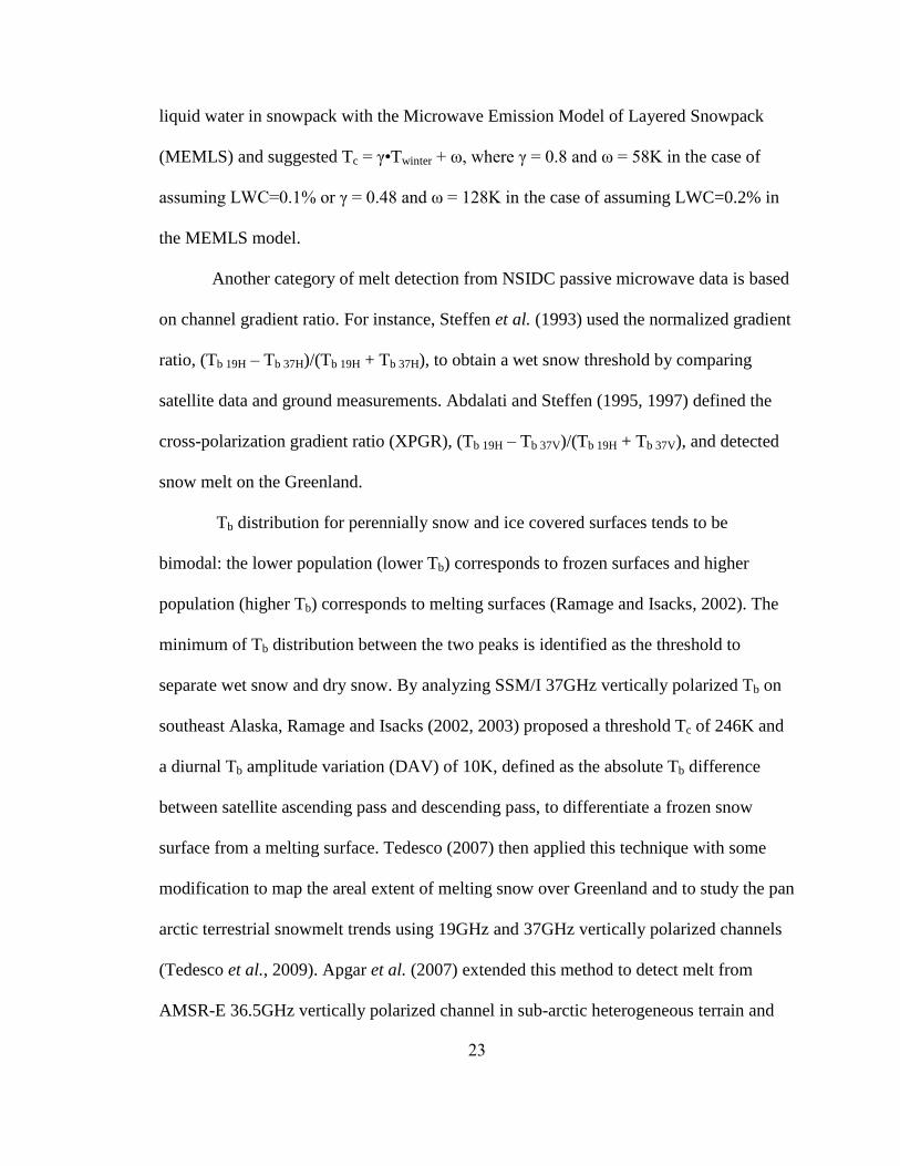
liquid water in snowpack with the Microwave Emission Model of Layered Snowpack
(MEMLS) and suggested Tc = γ•Twinter + ω, where γ = 0.8 and ω = 58K in the case of
assuming LWC=0.1% or γ = 0.48 and ω = 128K in the case of assuming LWC=0.2% in
the MEMLS model.
Another category of melt detection from NSIDC passive microwave data is based
on channel gradient ratio. For instance, Steffen et al. (1993) used the normalized gradient
ratio, (Tb 19H – Tb 37H)/(Tb 19H + Tb 37H), to obtain a wet snow threshold by comparing
satellite data and ground measurements. Abdalati and Steffen (1995, 1997) defined the
cross-polarization gradient ratio (XPGR), (Tb 19H – Tb 37V)/(Tb 19H + Tb 37V), and detected
snow melt on the Greenland.
Tb distribution for perennially snow and ice covered surfaces tends to be
bimodal: the lower population (lower Tb) corresponds to frozen surfaces and higher
population (higher Tb) corresponds to melting surfaces (Ramage and Isacks, 2002). The
minimum of Tb distribution between the two peaks is identified as the threshold to
separate wet snow and dry snow. By analyzing SSM/I 37GHz vertically polarized Tb on
southeast Alaska, Ramage and Isacks (2002, 2003) proposed a threshold Tc of 246K and
a diurnal Tb amplitude variation (DAV) of 10K, defined as the absolute Tb difference
between satellite ascending pass and descending pass, to differentiate a frozen snow
surface from a melting surface. Tedesco (2007) then applied this technique with some
modification to map the areal extent of melting snow over Greenland and to study the pan
arctic terrestrial snowmelt trends using 19GHz and 37GHz vertically polarized channels
(Tedesco et al., 2009). Apgar et al. (2007) extended this method to detect melt from
AMSR-E 36.5GHz vertically polarized channel in sub-arctic heterogeneous terrain and

24
suggested Tc and DAV to be 252K and 18K, respectively; Monahan and Ramage (2010)
then applied these thresholds to study snow melt regimes in the Southern Patagonia
Icefield.
To our knowledge, higher resolution MERSL-BYU SSM/I and AMSR-E data
have not been as frequently used in snowmelt studies. The resolution enhancement may
offer advantages for smaller ice covered areas and marginal regions. The bimodal Tb
distribution characteristic (Ramage and Isack, 2002, 2003) appears to hold for MERSL-
BYU SSM/I and AMSR-E data and therefore is used to help develop a data-appropriate
melt threshold in the following sections.
MERSL-BYU SSM/I melt signature algorithm
A consistent yearly threshold of 233K was determined from the annual MERSL-
BYU SSM/I 37GHz vertically polarized Tb distributions for 160 8.9×8.9 km2 pixel grids
on NovZ and 104 girds on SevZ (Fig. 6). MERSL-BYU SSM/I melt detection threshold
233K is much lower than earlier published thresholds for NSIDC SSM/I data, such as
246K for Alaska (Ramage and Isacks, 2002, 2003) and 258K for Greenland (Tedesco,
2007). In order to understand this difference, the current study presents a comparison
between the NSIDC and MERSL-BYU grids. Higher resolution MERSL-BYU SSM/I
images were resampled to 25×25 km2 EASE-Grid using area weighted average method.
Two representative full-glacier covered EASE-Grid pixels were randomly chosen for
illustration in the present work: pixel 1 (80˚30ʹN, 95˚24ʹE, mean elevation is 702m) on
SevZ and pixel 2 (75˚36ʹN, 61˚00ʹE, mean elevation is 760m) on NovZ (Fig. 4) (Digital

25
elevation model (DEM) is derived from the Global 30 Arc-Second Elevation Data Set
(GTOPO30)).
Linear Pearson coefficients of the two data sets for pixel 1 and 2 from 1996 to
2007 are computed in Table 3. Results show that the ascending passes (descending
passes) of NSIDC images are highly correlated with morning passes (evening passes) of
MERSL-BYU images. The NSIDC and MERSL-BYU Tb distributions of both pixels
(Fig. 7) indicate that MERSL-BYU Tb is generally 10-15K lower than NSIDC. This gap
might due to the different RSS data version processed by NSIDC and MERSL-BYU. The
threshold of 233K marks the minimum between the two populations of the MERSL-BYU
SSM/I Tb distributions (Fig. 7).
The threshold is 246K for NSIDC Tb (Fig. 7), which is identical to earlier
published work on Alaskan glaciers (Ramage and Isacks, 2002, 2003). Applying 246K as
threshold to NSIDC SSM/I daily maximum Tb data (Fig. 8), the MOD of pixel 1 (25×25
km2) in year 2000 corresponds to the earliest MOD of smaller eight MERSL-BYU SSM/I
pixels (8.9×8.9 km2) whose centers fell into the larger EASE-Grid, and the TMD,
although larger, is very close to the maximum of MERSL-BYU pixels (Table 4). The
smaller MERSL-BYU SSM/I derived TMD might be caused by the smoothing effect of
short and light melt events by the SIR technique. Therefore, current research suggests
resolution enhanced MERSL-BYU data are applicable for small ice caps on SevZ and
NovZ and tend to give a conservative estimate of TMD.
For most other studies, Tc and DAV were used together to map wet snow (e.g.
Ramage and Isacks, 2002, 2003; Tedesco, 2007; Tedesco et al., 2009). However, in
NovZ and SevZ, selected ice pixels usually have similarly high Tb values in daily

26
multiple observations during intense melt, which results in low DAV (Table 5). Current
research focused on the starting date of melt (MOD) and how many days melt occurred
(TMD). The daily maximum Tb metric is strong enough to differentiate wet and dry snow
and incorporating DAV could blur the MOD and TMD results. Therefore, the DAV
metric is not used in this research. Two possible reasons might account for the low DAV
during intense melt season: (1) sensor pass time failed to capture nocturnal refreezing; (2)
the polar day phenomenon exposed the snowpack under solar radiation all day long,
which might prevent the snowpack from refreezing completely at night.
The snowpack on NovZ and SevZ glaciers tends to melt intermittently with melt
and refreezing cycles in the entire ablation season. Daily maximum Tb of multiple passes
are used in order to capture daily melt to the greatest extent. Each pixel’s MOD is defined
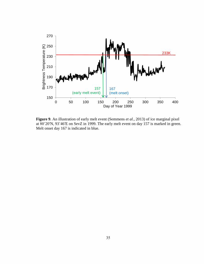
as the first day when 3 out of 5 consecutive days’ maximum Tb were higher than 233K.
Abnormally short early melt event, usually occurring at the end of accumulation season
but preceding ablation season, could affect the average ice melt onset timing (Fig. 9)
(Semmens et al., 2013). Therefore, current research defines the entire archipelago’s
MOD as the first day when more than 90% of the selected pixels melt. Each pixel’s TMD
is calculated as the total count of days with daily maximum Tb higher than 233K,
including early melt events.

27
Figure 6. Total brightness temperature distributions of MERSL-BYU SSM/I 37GHz
vertically polarized channel from 1996 to 2007. Back lines are distributions for SevZ and
blue lines are for NovZ. The most transparent black and blue curves show the earliest
year (1996) and the most opaque curves are the latest year (2007). The vertical red line
indicates the melt threshold of 233K for MERSL-BYU SSM/I. A total of 104 and 160
8.9×8.9 km2 grid pixels were analyzed each year on SevZ and NovZ, respectively.
0
500
1000
1500
2000
2500
3000
3500
4000
4500
140 190 240 290
Fre
quency
SSM/I Tb (K)
233K

28

29
Figure 7. Histograms of NSIDC and MERSL-BYU SSM/I 37GHz vertically polarized
brightness temperatures of the selected pixels from 1996 to 2007. Pixel 1 (80˚30ʹN,
95˚24ʹE) is on SevZ and Pixel 2 (75˚36ʹN, 61˚00ʹE) is on NovZ. Dashed black line is
threshold for MERSL-BYU data and solid black line is threshold for NSIDC data.
0
50
100
150
200
250
300
350
140 160 180 200 220 240 260 280
Fre
qu
en
cy
Brightness Temperature (K)
SevZ_NSIDC
SevZ_Regridded BYU
NovZ_NSIDC
NovZ_Regridded BYU
233K 246K

30
(a)
① ②
③ ④
⑤ ⑥
⑦ ⑧

31
(b)

32
Figure 8. Daily maximum Tb comparisons between NSIDC and MERSL-BYU SSM/I of
Pixel 1. (a) shows NSIDC SSM/I 25×25 km2
grid and MERSL-BYU 8.9×8.9 km2 grids.
MERSL-BYU original grid cells are numbered from ① to ⑧. The top panel of (b) is
NSIDC pixel and the following eight are MERSL-BYU original pixels as shown in (a).
Applying 246K as the threshold to detect melt from NSIDC pixel, it picks up the earliest
melt. Note that the vertical scale is different for the top panel of (b).

33
Table 4. Summary of Melt Onset Date, Refreeze Date and Total Melt Days of Pixels in
Fig. 8.
Pixel Melt Onset Date Refreeze Date Total Melt Days
NSIDC 182 240 46
MERSL-BYU ① 183 235 30
MERSL-BYU ② 183 235 36
MERSL-BYU ③ 183 235 37
MERSL-BYU ④ 183 240 37
MERSL-BYU ⑤ 182 236 38
MERSL-BYU ⑥ 183 240 30
MERSL-BYU ⑦ 183 240 43
MERSL-BYU ⑧ 183 240 42
* The unit for melt onset and refreeze date is “day of year 2000”. The unit for total melt days is “days”.

34
35
Figure 9. An illustration of early melt event (Semmens et al., 2013) of ice marginal pixel
at 80˚20ʹN, 93˚46ʹE on SevZ in 1999. The early melt event on day 157 is marked in green.
Melt onset day 167 is indicated in blue.
150
170
190
210
230
250
270
0 50 100 150 200 250 300 350 400
Brig
htn
ess T
em
pe
ratu
re (
K)
Day of Year 1999
233K
157 (early melt event)
167 (melt onset)

36
MERSL-BYU AMSR-E melt signature algorithm
MERSL-BYU AMSR-E data were processed from the same version of un-
resampled Tb as NSIDC processed Level 2A Tb (Gunn, 2007). MERSL-BYU AMSR-E
Tbs from 2003 to 2011 distributed bimodally with a yearly variable constant about 245K
on SevZ and 252K on NovZ (Fig. 10). The present work conservatively sets the melt
threshold to 252K for both areas, which has been compared with contemporaneous
MERSL-BYU SSM/I Tb as well as active microwave sensors in the results. This
threshold is also consistent with earlier published works (e.g., Apgar et al., 2007).
Consistent with MERSL-BYU SSM/I melt signature algorithm, each pixel’s
MOD is defined as the first day when 3 out of 5 consecutive days’ maximum Tb were
higher than 252K. The overall archipelago snowpack melt is defined as the first day when
90% of the selected pixels melt. Each pixel’s TMD is calculated as the total days with
daily maximum Tb higher than 252K.

37
Figure 10. Total brightness temperature distributions of MERSL-BYU AMSR-E
36.5GHz vertically polarized channel from 2003 to 2011. Back lines are distributions for
SevZ and blue lines are for NovZ. The most transparent black and blue curves show the
earliest year (2003) and the most opaque curves are the latest year (2011). The vertical
red line indicates the melt threshold of 252K for MERSL-BYU AMSR-E. A total of 104
and 160 8.9×8.9 km2 grid pixels were analyzed each year on SevZ and NovZ,
respectively.
0500
1000150020002500300035004000450050005500
140 190 240 290F
req
uen
cy
AMSR-E Tb (K)
252K

38
Active Microwave
Previous studies of melt detection from active scatterometer data are primarily
threshold based. Snowpack starts melting when drops below a threshold of M, defined
as - , where
is the winter average of (usually from January to
February) and is a region- and sensor-specific constant (e.g., Wismann, 2000; Smith et
al., 2003; Wang et al., 2005, 2007).
MERSL-BYU QSCAT melt signature algorithm
MERSL-BYU QSCAT data have been widely applied in monitoring melting
processes over major ice sheets over Greenland and Antarctic (e.g., Wang et al., 2007;
Trusel et al., 2012), small arctic ice caps (e.g., Wang et al., 2005), sea ice (e.g., Howell et
al, 2006), and mid-latitude mountain glaciers (e.g., Panday et al., 2011). Sharp and Wang
(2009) studied summer melt on Eurasian arctic ice caps including SevZ and NovZ using
the slice-based MERSL-BYU QSCAT data (2.225 2.225 km2) and established two
thresholds to detect melt by tuning with the Moderate Resolution Imaging
Spectroradiometer (MODIS) land surface temperatures. All periods when drops below
for one day using 1 = 5 dB or for consecutive three days using 2 = 3.5 dB are
classified as melt days.
Although lower resolution egg-based MERSL-BYU QSCAT data (4.45 4.45
km2) are used in this study, MODs derived via Sharp and Wang (2009)’s algorithm are
quite close to earlier published results on NovZ and SevZ (Table 6). Egg-based results
indicate a slightly later MOD and longer TMD than slice-based. The slight differences
are probably due to the fact that pixel selection in current study is more concentrated on

39
internal ice, which usually has a later MOD than lower elevation marginal ice. Analysis
also found that ice marginal pixels have significantly lower winter mean backscatter than
ice cap interiors, but have similar magnitude during summer melt, which Sharp and
Wang (2009) also noticed. This phenomenon would lead the fixed decrease algorithm
to underestimate the TMD for ice marginal pixels. Sharp and Wang (2009) included
many more marginal pixels than in this study and this is probably the reason why they
have a lower TMD. Despite the minor inconsistency, their algorithm is applied to the
entire lower resolution QSCAT data records to verify the passive microwave results in
the present study.

40

41
MERSL-BYU ERS-1/2 melt signature algorithm
Wismann (2000) detected melt based on ERS data for the Greenland ice sheet
assuming equals 3 dB, which corresponds to a top layer of 7 cm thickness having snow
moisture of 0.5%. Smith et al. (2003) used a dynamic threshold method to detect melt for
small Arctic ice caps with a couple of 25×25 km2 pixel grids in NovZ and SevZ.
However, the thresholds are not directly transferable to the resolution-enhanced images
(8.9×8.9 km2) in this research. Through theoretical modeling, Ashcraft and Long (2006)
suggested to be 1.0 dB for the MERSL-BYU ERS-1/2 data in Greenland. But they
found this threshold would create excessive false melt and modified it to 2.7 dB, which
has the highest melt detection consistency with QSCAT data.
The threshold of 2.7 dB tends to miss brief but significant melt events on NovZ
and SevZ. Through careful examination of backscatter variability compared to MERSL-
BYU SSM/I Tb and in-situ temperature record, a threshold of = 1.7 dB was empirically
determined and yields high MOD consistency with SSM/I algorithm here.
Due to lower temporal resolution, each pixel’s MOD is defined as the first day
when observations drop below the threshold M (
). Entire island MOD is
defined as the first day when more than 90% of selected pixels drop below the threshold
M.

42
MERSL-BYU ASCAT melt signature algorithm
Imaging at similar wavelength as ERS, ASCAT has potential in measuring
surface moisture and monitoring snow melt timing (Naeimi et al., 2012). In the present
analysis, ASCAT data are used to compare with MERSL-BYU AMSR-E time series
from 2009 to 2011 and provide the most updated MOD for 2012.
Through careful comparison with contemporaneous MERSL-BYU AMSR-E
(2009-2011) and QSCAT (2009) data, = 1.0 dB is determined in order to maintain
good MOD agreement with QSCAT and AMSR-E. This threshold is similar to what
Ashcraft and Long (2006) theoretically proposed for C-band ERS data.
In consistency with previous definitions, each pixel’s MOD from ASCAT is
defined as the first day when drops below the threshold M ( ) for 3 out of 5
consecutive days. Entire island MOD is defined as the first day when more than 90% of
selected pixels drop below the threshold M.
MERSL-BYU SSM/I and AMSR-E multi-overpass brightness temperatures as
well as ERS-1/2, QSCAT and ASCAT time series for selected pixels are programmed
in Interactive Data Language (IDL) to be automatically extracted and stored in text
arrays.

43
RESULTS
Sensor Time Series and In-situ Temperature Intercomparisons
MERSL-BYU SSM/I, ERS and in-situ temperature data
A time series of MERSL-BYU SSM/I daily maximum Tb and ERS at the
AWS location (80˚31ʹN, 94˚49ʹE) on SevZ are compared to above ground 2.5 meter daily
maximum air temperature record for the year 1999 (Fig. 11) (Opel et al., 2009). When air
temperature increased above 0˚C, SSM/I daily maximum Tb increased and ERS
dropped abruptly.
The threshold of 233 K for MERSL-BYU SSM/I data effectively separated
melting events from frozen state and only five days (Julian day 192, 221, 223, 241 and
242) were misclassified. The misclassification might be caused by the unrepresentative
point observation compared to the large area of the remote sensing measurement. It is
also likely that our melt assumption is not perfect (Liston and Winther, 2005; Trusel et
al., 2012): daily maximum temperature may briefly exceed 0˚C but surface energy
balance is negative and snowpack remains dry (situation of Julian day 221 and 223); or
conditions may be the reverse (situation of Julian day 192, 241 and 242). Genthon et al.
(2011) suggested that AWS temperature records could be significantly warm biased in
summer on Antarctic Plateau as a result of high incoming solar flux, high surface albedo,
and low wind speed. Although far insufficient in-situ observations are available to test
whether this bias existed on SevZ, inaccurate measurement could be additional reason for
the misclassification.

44
Figure 11. Time series comparison between MERSL-BYU SSM/I, ERS, and near-
surface (2.5 m above ground) air temperature in 1999 at AWS location (80˚31ʹN,
94˚49ʹE) (Opel et al., 2009). A threshold of 233K was used for MERSL-BYU SSM/I
37GHz vertically polarized brightness temperatures. Melt onset retrieved from MERSL-
BYU SSM/I algorithm is 184 and 181 from MERSL-BYU ERS algorithm.
0
50
100
150
200
250
300
-35
-30
-25
-20
-15
-10
-5
0
5
10
1 50 99 148 197 246 295 344
Brig
htn
ess T
em
pe
ratu
re (
K)
Ba
cksca
tte
r (
dB
)
Day of Year (1999)
233K
Te
mp
era
ture
(˚C)
184 181

45
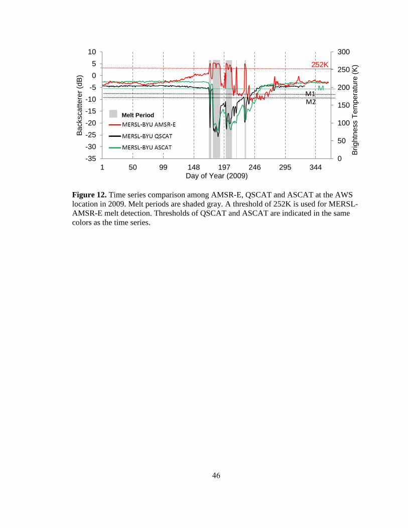
MERSL-BYU AMSR-E, QSCAT and ASCAT
MERSL-BYU AMSR-E 36.5 GHz vertically polarized Tb were compared to
QSCAT and ASCAT at AWS location (80˚31ʹN, 94˚49ʹE) in 2009 (Fig. 12). Abrupt
increase in AMSR-E Tb (>252K) corresponds to a sharp decrease in QSCAT and ASCAT
. Careful examination of every pixel’s behaviors between passive and active sensors
reveals that the threshold of 252K is effective in separating wet snow from dry state using
the MERSL-BYU AMSR-E 36.5 GHz vertically polarized brightness temperatures.
46
Figure 12. Time series comparison among AMSR-E, QSCAT and ASCAT at the AWS
location in 2009. Melt periods are shaded gray. A threshold of 252K is used for MERSL-
AMSR-E melt detection. Thresholds of QSCAT and ASCAT are indicated in the same
colors as the time series.
0
50
100
150
200
250
300
-35
-30
-25
-20
-15
-10
-5
0
5
10
1 50 99 148 197 246 295 344
Brig
htn
ess T
em
pe
ratu
re (
K)
Ba
cksca
tte
rer
(dB
)
Day of Year (2009)
252K
Melt Period
M M1 M2

47
Cross-validations of MOD and TMD among Sensors
In order to concatenate MOD and TMD from multiple sensors to create a long-
term record, it is important to cross validate melt detection results among sensors. The
frequency distribution of MOD difference between MERSL-BYU SSM/I and ERS from
1995 to 2000 (year 1996 was excluded from NovZ distribution because the ERS-1/2 data
gap missed this year’s MOD) on NovZ and SevZ indicates a mean value of 0.21, which
means the SSM/I algorithm generally detects melt 0.21 days later than ERS (Fig. 13 (a)).
The mean values of SevZ (red line) and NovZ (green line) distributions are 2.32 and -
1.43, respectively. Almost 90% of the differences fall within ± 6 days, which corresponds
to ERS observational uncertainty and lends confidence to the MOD derived from ERS for
1992-1994.
The frequency distribution of MOD difference between MERSL-BYU SSM/I and
QSCAT from 2000 to 2007 on both archipelagoes has a mean value of -0.18 days, which
means the MERSL-BYU SSM/I algorithm generally detects 0.18 days earlier than
QSCAT (Fig. 13 (b)). The mean values of SevZ and NovZ distributions are 0.38 and -
0.55 days, respectively.
The frequency distribution of MOD difference between MERSL-BYU SSM/I and
AMSR-E from 2003 to 2007 shows a mean value of -4.75 on NovZ and SevZ, which
means that MERSL-BYU SSM/I algorithm detects melt 4.75 days earlier than AMSR-E
(Fig. 13 (c)). This difference may be caused by the relatively strict threshold for AMSR-
E, especially for SevZ (Fig. 10). The mean values of SevZ and NovZ distributions are -
4.98 and -4.60, respectively.

48
The mean value of the frequency distribution of MOD difference between
MERSL-BYU AMSR-E and ASCAT from 2009 to 2011 is -1.41 days, which means
AMSR-E detects 1.41 days earlier than ASCAT (Fig. 13 (d)). The mean values of SevZ
and NovZ distributions are 6.09 and -6.28, respectively. The much higher mean values of
onset difference among SSM/I, AMSR-E and ASCAT on NovZ and SevZ indicates
different sensor sensitivity to the starting of main melt event significantly impacts the
mean MOD values, which further justifies the necessity of defining overall melt onset
date as the first day when more than 90% of selected pixels start melting.
MOD maps from different sensors are shown in Appendix A-E. The period of
2003-2007 has the most dense satellite overlap and a map comparison is done for
MERSL-BYU SSM/I, AMSR-E and QSCAT on both islands (Fig. 14 and Fig. 15).
Similar melt onset patterns exist between sensors despite the discrepancies among
different sensors.

49
(a) (b)
(c) (d)
Figure 13. Frequency distribution of MOD differences among sensors. (a) is the
frequency distribution of MOD difference between MERSL-BYU SSM/I and ERS from
1996 to 2007; (b) is the frequency distribution of MOD difference between MERSL-
BYU SSM/I and QSCAT from 2000 to 2009; (c) is the frequency distribution of MOD
difference between MERSL-BYU SSM/I and AMSR-E from 2003 to 2007; (d) is the
frequency distribution of MOD difference between MERSL-BYU AMSR-E and ASCAT
from 2009 to 2011. Black is NovZ and SevZ combined distribution; red and green are
distributions of SevZ and NovZ, respectively. Mean values of different distributions are
written in corresponding colors in the upper right corner of each plot.
0
0.05
0.1
0.15
0.2
0.25
-40 -30 -20 -10 0 10 20 30 40
No
rma
lize
d O
ccu
ren
ce
s
MOD SSM/I-ERS (days)
NovZ and SevZ
SevZ
NovZ
0
0.05
0.1
0.15
0.2
0.25
0.3
0.35
-40-30-20-10 0 10 20 30 40
No
rma
lize
d O
ccu
ren
ce
s
MOD SSM/I-QSCAT (days)
0
0.05
0.1
0.15
0.2
0.25
0.3
-40 -30 -20 -10 0 10 20 30 40
No
rma
lize
d O
ccu
ren
ce
s
MOD SSM/I-AMSRE (days)
0
0.05
0.1
0.15
0.2
0.25
0.3
0.35
0.4
-40 -30 -20 -10 0 10 20 30 40
No
rma
lize
d O
ccu
ren
ce
s
MOD AMSRE-ASCAT (days)
50

51

52
The frequency distribution of TMD difference between MERSL-BYU SSM/I and
QSCAT from 2000-2007 indicates a mean value of -10.1 days, which means that
MERSL-BYU QSCAT algorithm generally detects 10.1 more melt days than SSM/I on
both archipelagoes (Fig. 16 (a)). The mean values of SevZ and NovZ distributions are -
9.1 and -10.8, respectively. These differences are probably due to the fact that QSCAT
data is very sensitive to subsurface liquid water even when the ice is frozen (Steffen et
al., 2004; Hall et al., 2009). Incomplete refreezing of water in deep snow layers and the
capacity of firn to store water impede the active radar backscatter to return immediately
to its starting point when the air temperature drops below 0˚C, which questions the
reliability of snow melt days retrieved from scatterometer data (Wismann, 2000;
Rotschky et al., 2011). In view of this, TMD is conservatively estimated from MERSL-
BYU passive microwave (SSM/I and AMSR-E) from 1995 to 2011 for both
archipelagoes.
MERSL-BYU AMSR-E data had 8 missing observations during the intense melt
season in the year 2010. Those missing days are in the middle of melt and refreeze cycles
and the contemporaneous ASCAT signal did not show an increase in ; therefore the
present work assumes that melting occurred on those missing days and added 8 more
days to each pixel’s 2010 TMD for both NovZ and SevZ. The frequency distribution of
TMD difference between MERSL-BYU SSM/I and AMSR-E from 2003-2007 has a
mean value of 7.9 days, which means that the MERSL-BYU SSM/I algorithm generally
estimates 7.9 more melt days than AMSR-E on both archipelagoes. The mean values of
SevZ and NovZ distributions are 7.5 and 8.2 days, respectively (Fig. 16 (b)). These
positive differences might be caused by the relatively strict threshold for MERSL-BYU

53
AMSR-E Tb, which underestimates melt especially for SevZ (Fig. 10). The normal
distributions indicate that systematic error exists between MERSL-BYU SSM/I and
AMSR-E algorithms. The standard deviation of NovZ and SevZ frequency distribution of
TMD difference are 7.97 and 9.75 days, respectively, and 9.1 days for NovZ and SevZ
combined distribution. The different sensor sensitivity to wet snow, effective satellite
pass time and raw data footprint might account for the systematic error. Because of less
variability in melt detection threshold (Fig. 6) and good agreement with in-situ
temperature (Fig. 11), the present work corrected the systematic error in MERSL-BYU
AMSR-E data during 2008-2011 to SSM/I standard by adding 7.5 and 8.2 days to
AMSR-E-derived TMD on SevZ and NovZ, respectively (Bevington and Robinson,
1969).
TMD maps from MERSL-BYU SSM/I, AMSR-E and QSCAT are shown in
Appendix F-H. The period of 2003-2007 has the most dense satellite overlap and a map
comparison is done on both islands (Fig. 17 and Fig. 18). MERSL-BYU SSM/I and
AMSR-E have a relatively better consistency but QSCAT detects significantly more melt
days than SSM/I and AMSR-E algorithms, which is consistent with earlier discussions
(Fig. 16).

54
(a) (b)
Figure 16. Frequency distributions of TMD differences among sensors. (a) is the
frequency distribution of TMD difference between MERSL-BYU SSM/I and QSCAT
from 2000 to 2009. (b) is the frequency distribution of TMD difference between MERSL-
BYU SSM/I and AMSR-E from 2003 to 2007. Black is NovZ and SevZ combined
distribution; red and green are distributions of SevZ and NovZ, respectively. Mean values
of different distributions are written in corresponding colors in the upper right corner of
each plot.
0
0.01
0.02
0.03
0.04
0.05
-40 -30 -20 -10 0 10 20 30 40
No
rma
lize
d O
ccu
ren
ce
s
TMD SSM/I - QSCAT (days)
0
0.01
0.02
0.03
0.04
0.05
0.06
0.07
0.08
-40 -30 -20 -10 0 10 20 30 40
No
rma
lize
d O
ccu
ren
ce
s
TMD SSM/I - AMSR-E (days)
SevZ and NovZ
SevZ
NovZ

55

56

57
MOD and TMD Trend
Annual glacier surface MOD detected from multiple passive and active
microwave sensors are shown in Fig. 19 (a). A box plot of annual TMD from passive
microwave sensors is shown in Fig. 19 (b), in which the upper and lower error bars are
the maximum and minimum TMD, respectively; the three lines from the bottom to top
are the lower, median and upper quartile observations; dots in the boxes are the annual
mean value of the TMD. A data gap in MERSL-BYU ERS-1/2 from May 6th
to June 2nd
1996 missed a significant widespread melt event in NovZ on May 20th
. Therefore, ERS
derived MOD for 1996 was excluded in Fig. 19 (b).
Snowpack on SevZ and NovZ tends to melt intermittently with melting and
refreezing cycles in the entire ablation season. The average MOD is June 20th
(day of
year: 171) on SevZ and June 10th
(day of year: 161) on NovZ during 1992-2012. The
average TMDs are 47 and 67 days on SevZ and NovZ, respectively.
A statistically significant earlier MOD trend, about 0.73 days/year (p-value <
0.01), is observed for the glaciers on SevZ from multiple sensors during 1992 to 2012 by
regressing average values of each year’s available multi-satellite results (Fig. 19 (a)).
From passive microwave data, TMD on SevZ increased about 0.75 days/year (p-value <
0.05) from 1995 to 2011 (Fig. 19 (c)). In contrast, NovZ had large interannual variability
in MOD and no significant trend (Fig. 19 (b)). NovZ TMD increased although not as
significantly as SevZ (Fig. 19 (c)).

58
(a) (b)
(c)
Figure 19. Decadal variations in annual MOD and TMD. (a) and (b) are annual MOD of
icecaps in SevZ and NovZ, respectively, derived from multiple sensors from 1992 to
2012. A data gap in MERSL-BYU ERS-1/2 products missed a significant wide spread
melt event in NovZ on May 20th
, 1996; therefore the present work did not include 1996’s
ERS derived MOD in (b). (c) is a boxplot of passive microwaved based glacier TMD on
both archipelagoes from 1995 to 2011; Upper and lower error bars in (c) show the
maximum and minimum pixel based TMD.
y = -0.7331x + 1639 p-value < 0.01
120
130
140
150
160
170
180
190
1992 1996 2000 2004 2008 2012
Se
vZ
MO
D (
day o
f ye
ar)
Year
ERSSSM/IAMSREQSCATASCAT
120
130
140
150
160
170
180
190
1992 1996 2000 2004 2008 2012
No
vZ
MO
D (
day o
f ye
ar)
Year
ERSSSM/IAMSREQSCATASCAT
0
20
40
60
80
100
120
1995 1997 1999 2001 2003 2005 2007 2009 2011
To
tal N
um
be
r o
f M
elt D
ays
Year
y = 0.7534x - 1462 p-value < 0.05
y = 0.7085x -1352 p-value = 0.17
SevZ
NovZ

59
Relationships with Local Air Temperature
The present work found a strong positive relationship between annual mean TMD
and the average June-August NCEP-NCAR reanalysis air temperature (Kistler et al.,
2001) at a geopotential height of 850 hPa on both archipelagoes (Fig. 20 (a)), which is
consistent with what Sharp and Wang demonstrated based on a five year QSCAT melt
record (Sharp and Wang, 2009). The slope of the linear regression between annual mean
TMD and mean June-August 850 hPa air temperature is ~9.8 days/˚C (p < 0.0002) and
~8.1 days/˚C (p-value < 0.0001) in NovZ and SevZ respectively, indicating that NovZ
was more sensitive to temperature variation compared to SevZ in recent decades.
Reanalysis data indicate a more significant (p-value < 0.05) summer air temperature
increase in NovZ from 1995 to 2011. This temperature increase and higher sensitivity to
temperature change probably contribute to the larger ice mass loss rate in NovZ (~0.32
Mt a-1
km-2
) compared to SevZ (~0.08 Mt a-1
km-2
) between October 2003 and October
2009 (Moholdt et al., 2012). This higher sensitivity suggests icecaps on NovZ may be
more vulnerable to future temperature increase.
SevZ snowpack MOD has the highest correlation with June 850hPa geopotential
height NCEP-NCAR reanalysis air temperature compared to other months. This is
probably due to the fact that melting usually occurs in June for SevZ (Fig. 20 (b)).
However, NovZ snowpack MOD has no such relationship with any month’s reanalysis
temperature.

60
(a) (b)
Figure 20. Snowmelt relation with local reanalysis 850 hPa geopotential height
temperatures. (a) is relation between TMD and June-August mean reanalysis temperature.
(b) is relation between MOD and June mean reanalysis temperature. Blue and black dots
represent NovZ and SevZ, respectively. Regression functions, R2 and p-values are also
marked in corresponding colors.
y = 8.1111x + 72.23 R² = 0.685
p-value < 0.0001
y = 9.7936x + 81.378 R² = 0.615
p-value < 0.0002
20
30
40
50
60
70
80
90
-6 -4 -2 0 2
TM
D (
days)
850 hPa June-August Average Reanalysis Temperature (˚C)
y = -3.6326x + 156.23 R² = 0.3912
p-value < 0.005
y = -1.1327x + 158.37 R² = 0.031 120
130
140
150
160
170
180
190
200
-8 -6 -4 -2
MO
D (
day o
f ye
ar)
850 hPa June Average
Reanalysis Temperature (˚C)

61
Relationships with Local Sea Ice Extent
Recent decreases in sea ice extent are realized to be consistent with snowmelt
fluctuations in a pan-arctic perspective (Serreze et al., 2007). Rotschky et al. (2011)
discussed the possibility of local sea ice extent as a driving force for the glacier snowmelt
in Svalbard and found that, for some abnormal years, early snowmelt and long melt
duration is related to local anomalous low sea ice extent. The present work investigated
the possible relationship between the melting of NovZ and SevZ snowpack and local sea
ice extent derived from the National Snow and Ice Data Center (Cavalieri and Parkinson,
2012). Geographically, SevZ divides the Arctic Ocean and Kara & Barents Seas and
NovZ is in the middle of the Kara & Barents Seas (Fig. 1). Multiple linear regression
analysis reveals that SevZ TMD has a significant negative relationship with Arctic Ocean
September minimum sea ice extent (p-value < 0.01) from 1995 to 2010 (Fig. 21), but is
insignificantly related to Kara & Barents Seas. A statistically significant negative relation
(p-value < 0.05) between NovZ TMD and Kara & Barents annual minimum sea ice
extent from 1995 to 2009 is also found (Fig. 21). The year 2010 is an outlier with an
abnormally low Kara & Barents Seas sea ice extent but short NovZ snowpack TMD. This
can be explained by the cold anomaly right above NovZ, an exception to an abnormally
warm summer in 2010 for the rest of the Arctic as seen in Goddard Institute for Space
Studies (GISS) at National Aeronautics and Space Administration (NASA) surface
temperature analysis map (Fig. 22) (Hansen et al., 2010). The latent heat transported
from other warming Arctic environment might have caused Kara & Barents Seas sea ice
extent to reach an unusually low point in 2010 while the cold temperature over the island
made glacier melt a shorter than normal period.

62
The current research also investigated the potential relation between MOD and
regional sea ice extent; however, no statistically significant relation was discovered.

63
Figure 21. TMD relation with regional annual minimum sea ice extent. Black dots are
scatterplot between Arctic Ocean sea ice extent and SevZ TMD from 1995 to 2010. Blue
dots are scatterplot between Kara & Barents Seas sea ice extent with NovZ TMD from
1995 to 2009 and the blue square is the outlier year of 2010. Regression functions, R2 and
p-values are marked in corresponding colors. The upper blue x-axis is local sea ice extent
in Kara & Barents Seas and lower dark x-axis is local sea ice extent in Arctic Ocean.
y = -5.6x + 73.5 R² = 0.4338
p-value < 0.01
y = -36.3x + 75.6 R² = 0.4922
p-value < 0.005
0 0.2 0.4 0.6 0.8
20
30
40
50
60
70
80
90
0 5 10
Millions
TM
D (
days)
Local Sea Ice Extent (million km2)

64
Figure 22. 2010 summer (June-August) temperature anomaly compared to 1951-2000.
Study region is outlined with a black box. (Figure Courtesy: Goddard Institute for Space
Studies (GISS) at National Aeronautics and Space Administration (NASA); Hansen et
al., 2010)
˚C

65
DISCUSSION
Mass Balance
All published estimates for the mass balance in the Russian High Arctic are
slightly negative, ranging from 0 to -200 km m-2
a-1
during the period of 1930-1988
(Bassford et al., 2006; Zeeberg and Forman, 2001). By adding an additional 4-6 Gt a-1
mass loss due to iceberg calving, Moholdt et al. (2012) suggests an average long-term
mass budget rate between -5Gt a-1
and -15Gt a-1
for the period 1930-1990. However, no
in-situ mass budget programs were carried out since 1988 for this region. Recently, based
on the Gravity Recovery and Climate Experiment (GRACE) remote sensing
measurements, Jacob et al .(2012) suggests mass balance rates of -4 ± 2 Gt a-1
and -1 ± 2
Gt a-1
on NovZ and SevZ, respectively, between 2003 and 2010. Moholdt et al. (2012)
derives a higher mass balance rate of -7.1± 1.2 Gt a-1
on NovZ and -1.4 ± 0.9 Gt a-1
on
SevZ during October 2003 to October 2009 by combining ICESat laser altimetry and
GRACE data. The precipitation on both islands during 2004-2009 increased compared to
1980-2009 mean (Moholdt et al., 2012). The increasing TMD trend derived in the present
research might indicate more snowmelt loss and offset the effect of the increasing
precipitation trend, especially for SevZ with only slightly negative mass balance rate,
which is consistent with Moholdt et al. (2012)’s statement that the climate mass budget
rate in 2004-2009 was not substantially different from the average of 1980-2009 period.
The higher sensitivity of snowpack melt (TMD) to temperature increase and the

66
significant positive temperature anomaly (Fig. 20) might account for the much higher
mass loss rate on NovZ.
Ocean water serves as a major precipitation source in the RHA (Kotlyako et al.,
2010). The rapidly diminishing summer sea ice is exposing larger open ocean water to
evaporation, and possibly leading to the positive precipitation anomaly on NovZ and
SevZ in recent years. The anti-correlation between snowmelt days and regional sea ice
extent might cancel out some effect of the climate warming on glacier mass balance in
this region and help maintain the climatic mass budget in an equilibrium way (Moholdt et
al., 2012). However, precipitation influences on snow accumulation are very complex,
and insufficiently detailed snowfall and rainfall measurements severely limit further
investigations of the above inference.
Paleo Perspective
Ice core data from Akademii Nauk (AN) ice cap (Fig. 4) on SevZ covering the
period 1883-1998 indicate pronounced 20th
-century temperature changes, a strong rise in
the early 1990s with the absolute temperature maximum in the 1930s (Opel et al., 2009).
The early 1990s warming is also documented in coastal marine sedimentary record on
NovZ (Polyak et al., 2004). Because snowmelt days are highly correlated with regional
summer temperature, these evidences suggest strong glacier melt during the early 1900s.
Further evidence for the existence of an intense melt period during the early 1900s is the
strong increase of melt-layer content in the AN ice core at the beginning of 20th
century
(Opel et al., 2009). However, the melt-layer content declines significantly during the
period of 1970-2000 compared to 1960-1980 mean, indicating a less intense melt period.

67
The snowmelt result in the present work shows the SevZ snowmelt duration in the late
1990s was significantly lower than the first decade of 21st century, which might indicate
an abrupt warming on SevZ after 2000. The snowmelt on NovZ shows similar pattern
based on this research. A large increase in total melt days occurred in 2001 and in
subsequent years there are more total melt days than in the recorded period prior to 2001.
Therefore, year 2000 may be a turning point from a cold period (1970-2000) to a warm
period (2000-2011) on SevZ and NovZ. However, due to limited length of the satellite
record, it is difficult to be certain.
Limitations and Future Work
Satellites employed in the present work took data of earth surface at different
local times. The phase of water in the snowpack and the liquid water content (LWC) are
highly dependent on the time of day. Different satellite images represent unique
snowpack conditions at the satellite local pass time, which contribute to the discrepancies
in the MOD and TMD detection among sensors. For example, in the morning of July 14
and afternoon of July 16, 1999 (Fig. 23 (a)), the satellite data detected melt at the AWS
location, but the temporally nearest surface air temperature record was slightly below
0˚C. It is very likely that snowpack started melting as a result of negative surface energy
balance during those periods despite the slightly negative air temperatures. Actually, Tb
increase is not necessarily an instantaneous response to positive air temperature; instead,
it is a response to the existence of liquid water in the snowpack. By using daily maximum
Tb, the present work can capture daily melt to a maximum extent (Fig. 23 (b)). However,

68
daily maximum Tb may still miss days with melt event that have refrozen completely at
the corresponding satellite overpass time.
QSCAT is very sensitive to subsurface liquid water even though the surface
snowpack is frozen (e.g., Steffen et al., 2004). QSCAT detected melt on June 28, 2004 at
the AWS location; however, MERSL-BYU SSM/I and AMSR-E daily maximum Tb were
below their thresholds, indicating the surface was more likely in a frozen state (Fig.
23(b)). MERSL-BYU SSM/I and AMSR-E daily Tb magnitude had decreased one day
ahead, indicating refreezing process might already start on June 27, 2004. Actually,
QSCAT also
increased significantly on the same day although lower than the melt
threshold proposed by Sharp and Wang (2009) (Fig. 22(b)). This sluggish response to
frozen surface questions the reliability of TMD retrieved from QSCAT (Wismann, 2000;
Rotschky et al., 2011).
Despite the shortcomings of detecting TMD from QSCAT, its high sensitivity to
subsurface liquid water has been demonstrated to be useful in quantifying melt intensity
on Greenland and Antarctic large ice sheet through empirical positive degree day (PDD)
model (Wismann, 2000; Smith et al., 2003; Trusel et al., 2012). However, its physical
mechanism is poorly understood and its applicability to small icecaps needs further
examination. In addition to modeling from active microwave data, Mote (2003) applied
the PDD model to SSM/I passive microwave Tb and estimated runoff rates, mass balance
and elevation changes on the Greenland ice sheet. However, the saturation of Tb at a very
low fraction of LWC in snowpack limits in-depth physical modeling of snowmelt
intensity from passive microwave data. Microwave sensors rarely distinguish the melting

69
between earlier accumulated snow and new summer fallen snow (if there is any), thus
this research does not distinguish between old and new snow.
Future work involves testing the feasibility of PDD model based on both active
and passive microwave sensors for the small ice caps in the Russian High Arctic. By
comparing with mass budget from ICESat laser altimetry and GRACE gravimetry, it is
also possible to reconstruct mass balance variations back to 1980s taking advantage of
longer observational history of microwave sensors. New satellite missions like CryoSat-2
(launched in 2010), ICESat-2 (~2016) and GRACE Follow-On (~2016) should be
incorporated to more accurately monitor mass budget variability and further understand
the glacier response to climate change in this environment.

70
(a)
(b)
-6
-5
-4
-3
-2
-1
0
1
2
145
165
185
205
225
245
265
0 12 24 36 48 60 72 84
Air T
em
pe
ratu
re (°
C)
Brig
htn
ess T
em
pe
ratu
re (
K)
Hours since the Midnight of July 14, 1999
MERSL-BYU SSM/I
AWS Air Temperature
233
-30
-25
-20
-15
-10
-5
0
220
225
230
235
240
245
250
255
260
265
270
0 12 24 36 48 60 72 84 96
Ba
cksca
tte
r (d
B)
Brig
htn
ess T
em
pera
ture
(K
)
Hours since Midnight of June 25, 2004
MSERL-BYU SSM/I
MERSL-BYU AMSR-E
MERSL-BYU QSCAT
M(σwn0− 5.0)
252
233

71
Figure 23. Satellite observation comparisons at different local time of day. (a) is a
comparison between MERSL-BYU SSM/I Tb twice-daily observations and in-situ air
temperature data at the AWS location on SevZ from July 14 to July 17, 1999. (b) is a
comparison among MERSL-BYU SSM/I, AMSRE-E Tb twice-daily observations and
QSCAT at the AWS location from June 25 to June 28, 2004. Sensor melt thresholds
are marked in corresponding colors.

72
CONCLUSIONS
In this study, resolution-enhanced passive microwave data (SSM/I and AMSR-E)
and active scatterometer data (ERS, QSCAT and ASCAT) are synthesized to create a
decadal melt record for Novaya Zemlya and Severnaya Zemlya. Given the different
sensitivity to snow wetness, temporal resolutions, raw data footprints, frequencies and
melt detection methodologies, the high correlation among passive and active microwave
remote sensing datasets instills confidence in the results reported here.
The snowpack on SevZ and NovZ tends to melt intermittently, with melting and
refreezing cycles in the entire ablation season. The average glacier melt onset date is June
20th
on SevZ and June 10th
on NovZ during the period of 1992-2012. The average melt
days are 46 and 67 days on SevZ and NovZ, respectively. Earlier melt onset and longer
melt length on NovZ is consistent with the regional climate that NovZ is warmer and
wetter than SevZ. Generally, snowpack starts melting earlier and longer on the west coast
of two archipelagoes and progressively becomes later and shorter to the eastern side.
Higher elevation icecap interiors usually have later melt onset and shorter melt days than
marginal lower elevation glaciers. These spatial melt patterns are also in agreement with
the regional climate. NovZ has large year-to-year variability in melt onset date, but its
melt season generally increased. However, SevZ has experienced a significant earlier
melt onset (~0.73 days/year, p-value < 0.01) and longer melt length (~0.75 days/year, p-
value < 0.05) trends since early 1990s. Longer melt season trends on SevZ and NovZ
might indicate reduced mass balance for both archipelagoes in recent decades.

73
SevZ snowpack melt onset date is positively correlated to June 850hPa reanalysis
temperature and annual mean total melt days on both islands are highly correlated with
the 850 hPa reanalysis summer (June-August) mean air temperatures. Results also
indicate that NovZ was more sensitive than SevZ to temperature variations in the past
decades. This higher sensitivity, in combination with a more significant temperature
increase might lead to the much larger reported ice mass loss rate in NovZ (Moholdt et
al., 2012).
Snowmelt on SevZ is found to be negatively correlated to Arctic Ocean sea ice
extent fluctuations at a high significance level. Similarly strong negative relationship is
also documented between NovZ snowmelt and Kara & Barents Seas sea ice extent.
Rapidly diminishing sea ice is exposing more open ocean water to evaporation,
potentially increasing glacier accumulation on both islands. The anti-correlation between
snowmelt and sea ice extent might serve as a mechanism to offset some effect of the
regional warming and help maintain the climatic mass budget in an equilibrium way on
NovZ and SevZ.

74
REFERENCES
Abdalati, W. and K. Steffen (1995). Passive microwave-derived snow melt regions on the
Greenland Ice sheet. Geophysical Research Letters, 22:787-790, doi:
10.1029/95GL00433.
Abdalati, W. and K. Steffen (1997). Snowmelt on the Greenland ice sheet as derived
from passive microwave satellite data. Journal of Climate, 10:165-175, doi:
10.1175/1520-0442(1997)010<0165:SOTGIS>2.0.CO;2
Amante, C and B.W. Eakins (2009). ETOPO1 1Arc-minute global relief model:
procedures, data sources and analysis. NOAA Technical Memorandum NESDIS NGDC-
24, 19pp, March.
Apgar, J.D., J.M. Ramage, R.A. McKenney and W. Hanna (2007). AMSR-E algorithm
for snowmelt onset detection in subarctic Heterogeneous Terrain, Hydrological Process,
21:1587-1596, doi: 10.1002/hyp.6721.
Ashcraft, I.S. and D.G. Long (2006). Comparison of methods for melt detection over
Greenland using active and passive microwave measurements. International Journal of
Remote Sensing, 27:2469-2488, doi: 10.1080/01431160500534465.
Ashcroft, P. and F. Wentz (2003). AMSR-E/Aqua L2A Global Swath Spatially-
Resampled Brightness Temperatures. Version 2. [2003-2011]. Boulder, Colorado USA:
National Snow and Ice Data Center.
Attema, E.P.W. (1991). The active microwave instrument on-board the ERS-1 satellite.
Proceedings of the IEEE, 79: 791-799, doi: 10.1109/5.90158.
Bassford, R.P., M.J. Siegert and J.A. Dowdeswell (2006). Quantifying the mass balance
of ice caps on Severnaya Zemlya, Russian High Arctic II: Modeling the flow of the
Vavilov Ice Cap under the present climate. Arctic, Antarctic, and Alpine Research,
38:13-20, doi: 10.2307/4095822.
Belchansky, G.I., D.C. Douglas, I.N. Mordvintsev and N.G. Platonov (2004). Estimating
the time of melt onset and refreeze onset over Arctic sea-ice area using active and passive
microwave data. Remote Sensing of Environment, 92: 21-39, doi:
http://dx.doi.org/10.1016/j.rse.2004.05.001.
Bevington, P. and D.K. Robinson (1969). Data reduction and error analysis for the
physical sciences. Published by McGraw-Hill Science/Engineering/Math (3rd
edition):
336pp.

75
Cavalieri, D.J., P. Gloersen and W.J. Campbell (1984). Determination of sea ice
parameters with the NIMBUS 7 SMMR. Journal of Geophysical Research, 89:5355-
5369, doi: 10.1029/JD089iD04p05355.
Cavalieri D.J. and C.L. Parkinson (2012). Arctic sea ice variability and trends, 1979-
2010. The Cryosphere, 6:881-889, doi: 10.5194/tc-6-881-2012.
Dowdeswell, J.A. and J.O. Hagen (2004). Mass Balance of the Cryosphere, J. Bamber
and A.J. Payne (eds.), Cambridge University Press: 712pp.
Drobot, S.D. and M.R. Anderson (2001). An improved method for determining snowmelt
onset dates over Arctic sea ice using scanning multichannel microwave radiometer and
Special Sensor Microwave/Imager data. Journal of Geophysical Research, 106:24,033-
24,049, doi: 10.1029/2000JD000171.
Early, D.S. and D.G. Long (2001). Image reconstruction and enhanced resolution
imaging from irregular samples. IEEE Transactions on Geoscience and Remote Sensing,
39:291-302, doi: 10.1109/36.905237.
Figa-Saldaña, J., J.J.W. Wilson, E. Attema, R. Gelsthorpe, M.R. Drinkwater and A.
Stoffelen (2002). The advanced scatterometer (ASCAT) on the meteorological
operational (MetOp) platform: A follow on for European wind scatterometers. Canadian
Journal of Remote Sensing, 28:404-412, doi: 10.5589/m02-035.
Gardner, A.S., G. Moholdt, B. Wouters, G.J. Wolken, D.O. Burgess, M.J. Sharp, J.G.
Cogley, C. Braun and C. Labine (2011). Sharply increased mass loss from glaciers and
ice caps in the Canadian Arctic Archipelago. Nature, 473: 357-360, doi:
10.1038/nature10089.
Genthon, C., D. Six, V. Favier, M. Lazzara and L. Keller (2011). Atmospheric
temperature measurement biases on the Antarctic Plateau. Journal of Atmospheric and
Oceanic Technology, 28:1598-1605, doi: 10.1175/JTECH-D-11-00095.1.
Gunn, B.A. (2007). Temporal resolution enhancement for AMSR images. Microwave
Earth Remote Sensing Laboratory, Brigham Young University, USA, December.
Hall, D.K., S.V. Nghiem, C.B. Schaaf, N.E. DiGirolamo and G. Neumann (2009).
Evaluation of surface and near-surface melt characteristics on the Greenland ice sheet
using MODIS and QuikSCAT data. Journal of Geophysical Research, 114, F04006, doi:
10.1029/2009JF001287.
Hansen, J., R. Ruedy, M. Sato and K. Lo (2010). Global surface temperature change.
Reviews of Geophysics, 48, RG4004, doi: 10.1029/2010RG000345.

76
Hinse, M., Q.H.J. Gwyn and L. Cimino (1988). Radiometric correction of C-band
imagery for topographic effects in regions of moderate relief. IEEE Transactions on
Geosciences and Remote Sensing, 26:122-132, doi: 10.1109/36.3012.
Howell, S.E.L., A. Tivy, J.J. Yackel and R.K. Scharien (2006). Application of a
SeaWinds/QuikSCAT sea ice melt algorithm for assessing melt dynamics in the
Canadian Arctic Arhipelago. Journal of Geophysical Research, 111, C07025, doi:
10.1029/2005JC003193.
Intergovernmental Panel on Climate Change (IPCC) (2001). Climate Change 2001:
Synthesis Report. A contribution of Working Groups I, II, and III to the Third
Assessment Report of the Intergovernmental Panel on Climate Change [Watson, R.T. and
the Core Writing Team (eds.)]. Cambridge University Press, Cambridge, United
Kingdom, and New York, NY, USA, 398pp.
Intergovernmental Panel on Climate Change (IPCC) (2007). Climate Change 2007:
Synthesis Report. Contribution of Working Group I, II, and III to the Fourth Assessment
Report of the Intergovernmental Panel on Climate Change [Core Writing Team,
Pachauri, R.K and Reisinger, A. (eds.)]. IPCC, Geneva, Switzerland, 104pp.
Jacob, T., J. Wahr, W.T. Pfeffer and S. Swenson (2012). Recent contributions of glaciers
and ice caps to sea level rise. Nature, 482:514-518, doi:10.1038/nature10847.
Kistler, R., E. Kalnay, W. Collins, S. Saha, G. White, J. Woollen, M. Chelliah, W.
Ebisuzaki, M. Kanamitsu, V. Kousky, H. van den Dool, R. Jenne and M. Fiorino (2001).
The NCEP-NCAR 50-year reanalysis: monthly means CD-ROM and documentation.
Bulletin of the American Meteorological Society, 82:247-267, doi: 10.1175/1520-
0477(2001)082<0247:TNNYRM>2.3.CO;2.
Kotlyako, V.M., A.M. Dyakova, V.S. Koryakin, V.I. Kravtsova, G.B. Osipova, G.M.
Varnakova, V.N. Vinogradov, O.N. Vinogradov and N.M. Zverkova (2010).
GLACIERS OF ASIA-GLACIERS OF THE FORMER SOVIET UNION (ed. Williams,
R.S., Jr., & Ferrigno, J.G.) (U.S. Government Printing Office.).
Lindsley, R.D. and D.G. Long (2010). Standard BYU ASCAT land/ice image products.
Microwave Earth Remote Sensing Laboratory, Brigham Young University, USA, June.
Liston, G.E. and J.G. Winther (2005). Antarctic surface and subsurface snow and ice melt
fluxes. Journal of Climate, 18:1469-1481, doi: 10.1175/JCLI3344.1.
Long, D.G. and D.L. Daum (1998). Spatial resolution enhanced SSM/I data. IEEE
Transactions on Geoscience and Remote Sensing, 36:407-417, doi: 10.1109/36.662726.

77
Long, D.G. and B.R. Hicks (2010). Standard BYU QuickSCAT and seawinds land/ice
image products. Microwave Earth Remote Sensing Laboratory, Brigham Young
University, USA, August.
Marshall, G.J., J.A. Dowdeswell and W.G. Rees (1994). The spatial and temporal effect
of cloud cover on the acquisition of high quality landsat imagery in the European Arctic
sector. Remote Sensing of Environment, 50:149-160, doi: http://dx.doi.org/10.1016/0034-
4257(94)90041-8.
Maslanik, J. and J. Stroeve (1990). Updated current year. DMSP SSM/I-SSMIS Daily
Polar Gridded Brightness Temperatures. Version 4.0. [1995-2007]. Boulder, Colorado
USA: National Snow and Ice Data Center.
Mätzler, C. (1994). Passive microwave signatures of landscapes in winter. Meteorology
and Atmospheric Physics, 54:241-260, doi: 10.1007/BF01030063.
Moholdt, G., C. Nuth, J.O. Hagen and J. Kohler (2010). Recent elevation changes of
Svalbard glaciers derived from ICESat laser altimetry. Remote Sensing of Environment,
114:2756-2767, doi: http://dx.doi.org/10.1016/j.rse.2010.06.008.
Moholdt, G., B. Wouters and A.S. Gardner (2012). Recent mass changes of glaciers in
the Russian High Arctic. Geophysical Research Letters, 39, L10502, doi:
10.1029/2012GL051466.
Monahan, P.A. and J. Ramage (2010). AMSR-E melt patterns on the Southern Patagonia
Icefield. Journal of Glaciology, 56:699-708, doi: 10.3189/002214310793146197.
Mote, T.L. and M.R. Anderson (1995). Variations in snowpack melt on the Greenland ice
sheet based on passive-microwave measurements. Journal of Glaciology, 41:51-60.
Mote, T. (2003). Estimation of runoff rates, mass balance, and elevation changes on the
Greenland ice sheet from passive microwave observations. Journal of Geophysical
Research, 108, 4056, doi:10.1029/2001JD002032.
Mote, T.L. (2007) Greenland surface melt trends 1973-2007:Evidence of a large increase
in 2007. Geophysical Research Letters, 34, L22507, doi: 10.1029/2007GL031976.
Naeimi, V., C. Paulik, A. Bartsch, W. Wagner, R. Kidd, S.E. Park, K. Elger and J. Boike
(2012). ASCAT surface state flag (SSF): Extracting information on surface freeze/thaw
conditions from backscatter data using an empirical threshold-analysis algorithm. IEEE
Transactions on Geoscience and Remote Sensing, 50:2566-2582, doi:
10.1109/TGRS.2011.2177667.

78
National Oceanic and Atmospheric Administration (NOAA) Earth System Research
Laboratory (ESRL), “Atmospheric Variables Plotting Page”, accessed April 24, 2013.
URL: http://www.esrl.noaa.gov/psd/data/histdata/.
Nick, F.M., A. Vieli, I.M. Howat and I. Joughin (2009). Large-scale changes in
Greenland outlet glacier dynamics triggered at the terminus. Nature Geoscience, 2:110-
114, doi: 10.1038/ngeo394.
Opel, T., D. Fritzsche, H. Meyer, R. Schütt, K. Weiler, U. Ruth, F. Wilhelms and H.
Fischer (2009). 115 year ice-core data from Akademii Nauk ice cap, Severnaya Zemlya:
high-resolution record of Eurasian Arctic climate change, Journal of Glaciology, 55: 21-
31, doi: 10.3189/002214309788609029.
Panday, P.K., K. E. Frey and B. Ghimire (2011). Detection of the timing and duration of
snowmelt in the Hindu Kush-Himalaya using QuikSCAT, 2000-2008. Environmental
Research Letters, 6, 024007, doi: 10.1088/1748-9326/6/2/024007.
Polyak, L., I. Murdmaa and E. Ivanova (2004). A high-resolution, 800-year glaciomarine
record from Russkaya Gavan’, a Novaya Zemlya fjord, eastern Barents Sea. The
Holocene, 14:638-644, doi: 10.1191/0959683604hl740rr.
Ramage, J.M. and B.L. Isacks (2002). Determination of melt-onset and refreeze timing
on southeast Alaskan icefields using SSM/I diurnal amplitude variations. Annals of
Glaciology, 34:391-398, doi: 10.3189/172756402781817761.
Ramage, J.M. and B.L. Isacks (2003). Interannual variations of snowmelt and refreeze
timing on southeast-Alaskan icefields, U.S.A. Journal of Glaciology, 49:102-116, doi:
10.3189/172756503781830908
Raup, B., A. Racoviteanu, S.J.S. Khalsa, C. Helm, R. Armstrong and Y. Arnaud (2007).
The GLIMS geospatial glacier database: A new tool for studying glacier change. Global
and Planetary Change, 56, 101-110, doi:
http://dx.doi.org/10.1016/j.gloplacha.2006.07.018.
Rotschky, G., T.V. Schuler, J. Haarpaintner, J. Kohler and E. Isaksson (2011). Spatio-
temporal variability of snowmelt across Svalbard during the period 2000-08 derived from
QuikSCAT/SeaWinds scatterometry. Polar Research, 30, 5963, doi:
10.3402/polar.v30i0.5963.
Screen, J.A. and I. Simmonds (2010). The central role of diminishing sea ice in recent
Arctic temperature amplification. Nature, 464:1334-1337, doi: 10.1038/nature09051.
Semmens, K.A., J. Ramage, A. Bartsch and G.E. Liston (2013). Early snowmelt events:
detection, and significance in a major sub-arctic watershed. Environmental Research
Letters, 8, 014020, doi: 10.1088/1748-9326/8/1/014020.

79
Serreze, M.C., M.M. Holland, J. Stroeve (2007). Perspectives on the Arctic’s shrinking
sea-ice cover. Science, 315:1533-1536, doi: 10.1126/science.1139426.
Sharp, M. and L. Wang (2009). A five-year record of summer melt on Eurasian Arctic ice
caps. Journal of Climate, 22(1):133-145, doi: 10.1175/2008JCLI2425.1.
Smith, L.C., Y. Sheng, R.R. Forster, K. Steffen, K.E. Frey and D.E. Alsdorf (2003).
Melting of small Arctic ice caps observed from ERS scatterometer time series.
Geophysical Research Letters, 30, 2034, doi: 10.1029/2003GL017641.
Steffen, K., W. Abdalati, and J. Stroeve (1993). Climate sensitivity studies of the
Greenland ice sheet using AVHRR, SMMR, SSM/I and in situ data. Meteorology and
Atmospheric Physics, 51:239-258, doi: 10.1007/BF01030497.
Steffen, K., S.V. Nghiem, R. Huff and G. Neumann (2004). The melt anomaly of 2002 on
the Greenland ice sheet from active and passive microwave satellite observations.
Geophysical Research Letters, 31, L20402, doi: 10.1029/2004GL020444.
Stiles, W.H. and F.T. Ulaby (1980). The active and passive microwave response to snow
parameters: 1. Wetness. Journal of Geophysical Research, 85:1037-1044, doi:
10.1029/JC085iC02p01037.
Takala, M., J. Pulliainen, S.J. Metsämäki and J.T. Koskinen (2009). Detection of
snowmelt using spaceborne microwave radiometer data in Eurasia from 1979 to 2007.
IEEE Transactions on Geoscience and Remote Sensing, 47:2996-3007, doi:
10.1109/TGRS.2009.2018442.
Tedesco, M. (2007). Snowmelt detection over the Greenland ice sheet from SSM/I
brightness temperature daily variations. Geophysical Research Letters, 34, L02504, doi:
10.1029/2006GL028466.
Tedesco, M. (2009). Assessment and development of snowmelt retrieval algorithms over
Antarctic from K-band spaceborne brightness temperature (1979-2008). Remote Sensing
of Environment, 113:979-997, doi: http://dx.doi.org/10.1016/j.rse.2009.01.009.
Tedesco, M., M. Brodzik, R. Armstrong, M. Savoie and J. Ramage (2009). Pan arctic
terrestrial snowmelt trends (1979-2008) from spaceborne passive microwave data and
correlation with the Arctic Oscillation. Geophysical Research Letters, 36, L21402, doi:
10.1029/2009GL039672.
Thomas, R.H., W. Abdalati, E. Frederick, W.B. Krabill, S. Manizade and K. Steffen
(2003). Investigation of surface melting and dynamic thinning on Jakobshavn Isbræ,
Greenland. Journal of Glaciology, 49: 231-239, doi: 10.3189/172756503781830764.

80
Torinesi, O., M. Fily, and C. Genthon (2003). Variability and trends of the summer melt
period of Antarctic ice margins since 1980 from microwave sensors. Journal of Climate,
16:1047-1060, doi: 10.1175/1520-0442(2003)016<1047:VATOTS>2.0.CO;2.
Trusel, L.D., K.E. Frey and S.B. Das (2012). Antarctic surface melting dynamics:
Enhanced perspectives from radar scatterometer data. Journal of Geophysical Research,
117, F02023, doi: 10.1029/2011JF002126.
Tsai, W.Y., S.V. Nghiem, J.N. Huddleston, M.W. Spencer, B.W. Stiles and R.D. West
(2000). Polarimetric scatterometry: a promising technique for improving ocean surface
wind measurements from space. IEEE Transactions on Geoscience and Remote Sensing,
38:1903-1921, doi: 10.1109/36.851773.
van den Broeke, M. (2005). Strong surface melting preceded collapse of Antarctic
Peninsula ice shelf. Geophysical Research Letters, 32, L12815, doi:
10.1029/2005GL023247.
Velicogna, I. (2009). Increasing rates of ice mass loss from the Greenland and Antarctic
ice sheets revealed by GRACE. Geophysical Research Letters, 36, L19503, doi:
10.1029/2009GL040222.
Wang, L., M.J. Sharp, B. Rivard, S. Marshall and D. Burgess (2005). Melt season
duration on Canadian Arctic ice caps, 2000-2004. Geophysical Research Letters, 32,
F19502, doi:10.1029/2005GL023962.
Wang, L., M. Sharp, B. Rivard and K. Steffen (2007). Melt season duration and ice layer
formation on the Greenland ice sheet, 2000-2004. Journal of Geophysical Research, 112,
F04013, doi: 10.1029/2007JF000760.
Weller, G., E. Bush, T.V. Callaghan, R. Corell, S. Fox, C. Furgal, A.H. Hoel, H.
Huntington, E. Kӓllén, V.M. Kattsov, D.R. Klein, H. Loeng, M.L. Martello,
M.MacCracken, M. Nuttall, T.D. Prowse, L. Reiersen, J.D. Reist, A. Tanskanen, J.E.
Walsh, B. Weatherhead, F.J. Wrona (2005) in Arctic Climate Assessment (ed. Symon,
C., Arris, L. and Heal, B.) Chapter 18. Cambridge University Press.
Wismann, V. (2000). Monitoring of seasonal snowmelt on Greenland with ERS
scatterometer data. IEEE Transactions on Geoscience and Remote Sensing, 38:1821-
1826, doi: 10.1109/36.851766.
Zeeberg, J. and S.L. Forman (2001). Changes in glacier extent on north Novaya Zemlya
in the twentieth century. The Holocene, 11:161-175, doi: 10.1191/095968301676173261.
Zwally, H.J., W. Abdalati, T. Herring, K. Larson, J. Saba and K. Steffen (2002). Surface
melt-induced acceleration of Greenland ice-sheet flow. Science, 297:218-222, doi:
10.1126/science.1072708.

81
APPENDIX A: MERSL-BYU SSM/I MOD maps from 1995 to 2007. Grid
size is 8.9×8.9 km2.
1995
1996
1997
130 200
Unit: day of year
144 192
Unit: day of year

82
1998
1999
2000
130 200
Unit: day of year
144 192
Unit: day of year

83
2001
2002
2003
130 200
Unit: day of year
144 192
Unit: day of year

84
2004
2005
2006
130 200
Unit: day of year
144 192
Unit: day of year
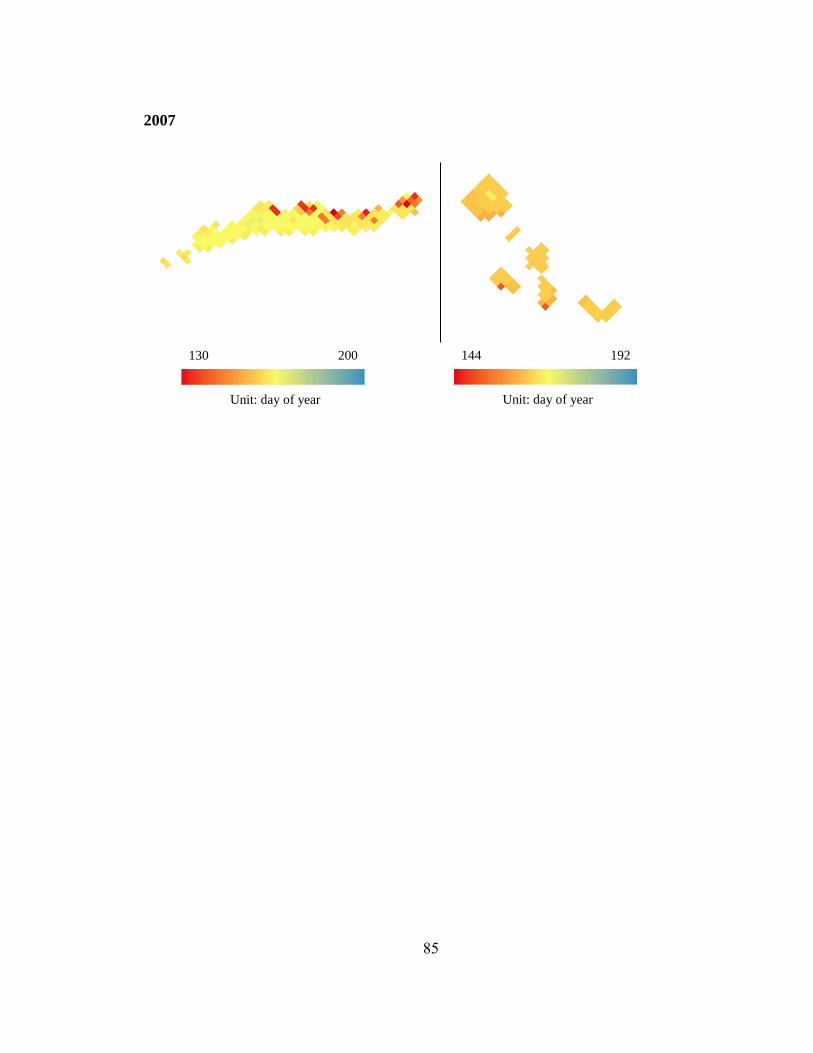
85
2007
130 200
Unit: day of year
144 192
Unit: day of year

86
APPENDIX B: MERSL-BYU AMSR-E MOD maps from 2003 to 2011.
Grid size is 8.9×8.9 km2.
2003
2004
2005
130 200
Unit: day of year
144 192
Unit: day of year

87
2006
2007
2008
130 200
Unit: day of year
144 192
Unit: day of year

88
2009
2010
2011
130 200
Unit: day of year
144 192
Unit: day of year

89
APPENDIX C: MERSL-BYU ERS MOD maps from 1992 to 2000. Grid
size is 8.9×8.9 km2.
1992
1993
1994
130 200
Unit: day of year
144 192
Unit: day of year

90
1995
1996
1997
130 200
Unit: day of year
144 192
Unit: day of year

91
1998
1999
2000
130 200
Unit: day of year
144 192
Unit: day of year

92
APPENDIX D: MERSL-BYU QSCAT MOD maps from 2000 to 2009.
Grid size is 4.45×4.45 km2.
2000
2001
2002
130 200
Unit: day of year
144 192
Unit: day of year

93
2003
2004
2005
130 200
Unit: day of year
144 192
Unit: day of year

94
2006
2007
2008
130 200
Unit: day of year
144 192
Unit: day of year

95
2009
130 200
Unit: day of year
144 192
Unit: day of year

96
APPENDIX E: MERSL-BYU ASCAT MOD maps from 2009 to 2012.
Grid size is 4.45×4.45 km2.
2009
2010
2011
130 200
Unit: day of year
144 192
Unit: day of year
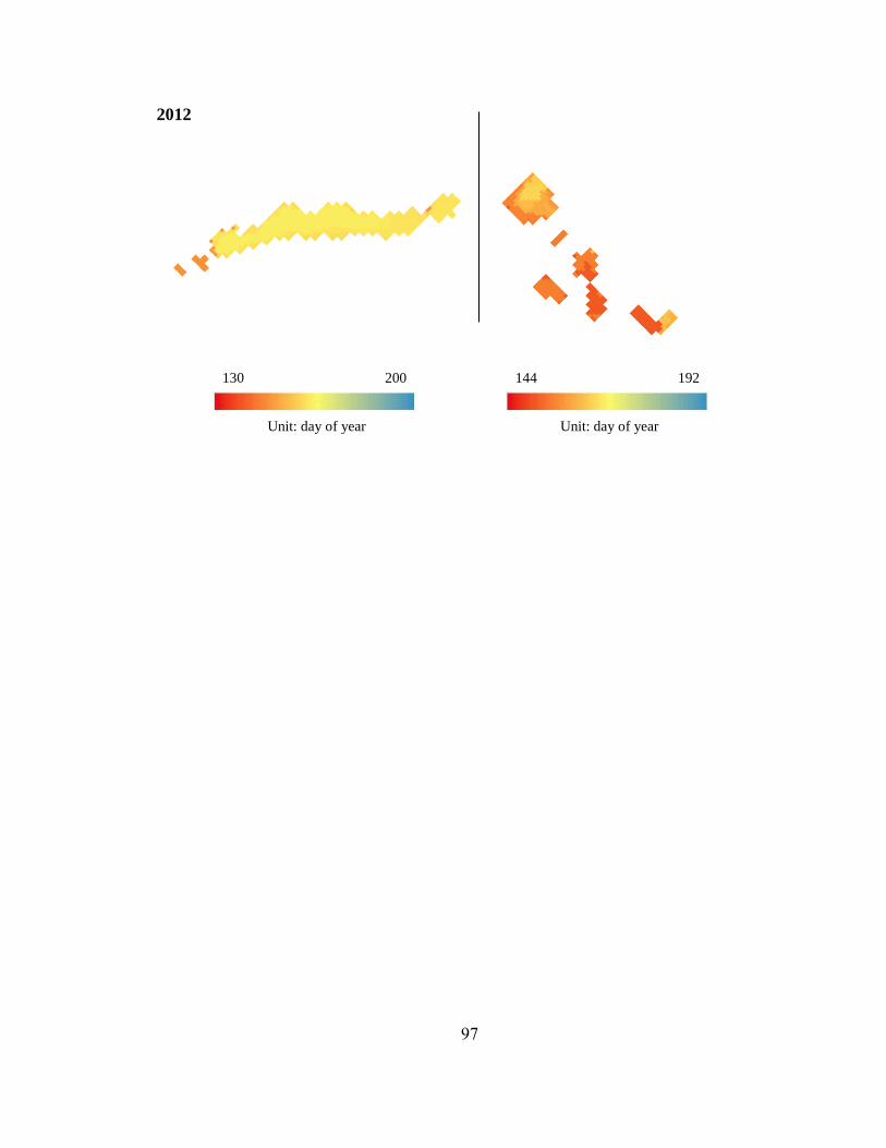
97
2012
130 200
Unit: day of year
144 192
Unit: day of year

98
APPENDIX F: MERSL-BYU SSM/I TMD maps from 1995 to 2007. Grid
size is 8.9×8.9 km2.
1995
1996
1997
29 120
Unit: days
16 75
Unit: days

99
1998
1999
2000
29 120
Unit: days
16 75
Unit: days

100
2001
2002
2003
29 120
Unit: days
16 75
Unit: days

101
2004
2005
2006
29 120
Unit: days
16 75
Unit: days

102
2007
29 120
Unit: days
16 75
Unit: days

103
APPENDIX G: MERSL-BYU AMSR-E TMD maps from 2003 to 2011.
Grid size is 8.9×8.9 km2.
2003
2004
2005
29 120
Unit: days
16 75
Unit: days

104
2006
2007
2008
29 120
Unit: days
16 75
Unit: days

105
2009
2010
2011
29 120
Unit: days
16 75
Unit: days

106
APPENDIX H: MERSL-BYU QSCAT TMD maps from 2000 to 2009.
Grid size is 4.45×4.45 km2.
2000
2001
2002
29 120
Unit: days
16 75
Unit: days

107
2003
2004
2005
29 120
Unit: days
16 75
Unit: days

108
2006
2007
2008
29 120
Unit: days
16 75
Unit: days

109
2009
29 120
Unit: days
16 75
Unit: days

110
Curriculum Vitae
Meng Zhao ([email protected])
EDUCATION
Lehigh University, Bethlehem, Pennsylvania, U.S.
Earth and Environmental Sciences, Master of Science, expected May, 2013
Wuhan University, Wuhan, Hubei, P.R.C.
Remote Sensing Science and Technology, Bachelor of Engineering, June 2011.
PROFESSIONAL EXPERIENCES
Graduate Student, Lehigh University
2013 Midwest Glaciology Meeting Oral Presentation: “Recent glacier surface
snowpack melt in the Novaya Zemlya and Severnaya Zemlya derived from active and
passive microwave remote sensing data”, University Park, PA, 5-8 March 2013.
American Geophysical Union 2012 fall meeting poster session: “Glacier surface
melt characterization and trend analysis (1992-2011) in the Russian High Arctic from
combined resolution-enhanced scatterometer and passive microwave data”, San
Francisco, CA, 3-7 December 2012.
69th
Eastern Snow Conference poster session: “Melt patterns of glaciers in Hindu
Kush-Himalayas (HKH) based on passive microwave data (AMSR-E)”, Claryville, NY, 6
June 2012.
Undergraduate Student, Wuhan University
Principal investigator of national undergraduate research project: “Computer-
based automatic water region delineation and extraction from RGB areophotograph”,
first-class award by the Ministry of Education of People’s Republic of China.
Publication: Zhao, M., H. Shang, W. Huang, L. Zou and Y. Zhang (2011). Water
area extraction from RGB aerophotograph based on chromatic and textural analysis.
Proceedings of the third international conference on advanced geographic information
systems, applications, and services. Gosier, Guadeloupe, France, pp. 46-52.
Undergraduate thesis: “Drought monitoring and assessment in Northern China
based on MODIS data”.