Portland State University Portland State University

PDXScholar PDXScholar

Dissertations and Theses Dissertations and Theses

Winter 2-23-2018

Recent Advances in Activity-Based Travel Demand Recent Advances in Activity-Based Travel Demand

Models for Greater Flexibility Models for Greater Flexibility

Kihong Kim Portland State University

Follow this and additional works at: https://pdxscholar.library.pdx.edu/open_access_etds

Part of the Transportation Commons, and the Urban Studies Commons

Let us know how access to this document benefits you.

Recommended Citation Recommended Citation Kim, Kihong, "Recent Advances in Activity-Based Travel Demand Models for Greater Flexibility" (2018). Dissertations and Theses. Paper 4225. https://doi.org/10.15760/etd.6109

This Dissertation is brought to you for free and open access. It has been accepted for inclusion in Dissertations and Theses by an authorized administrator of PDXScholar. Please contact us if we can make this document more accessible: pdxscholar@pdx.edu.

Recent Advances in Activity-Based Travel Demand Models for

Greater Flexibility

by

Kihong Kim

A dissertation submitted in partial fulfillment of the

requirements for the degree of

Doctor of Philosophy

in

Urban Studies

Dissertation Committee:

James Strathman, Chair

Liming Wang

Kelly Clifton

Wayne Wakeland

Portland State University

2018

© 2018 Kihong Kim

i

Abstract

Most existing activity-based travel demand models are implemented in a tour-based

microsimulation framework. Due to the significant computational and data storage

benefits, the demand microsimulation allows a greater amount of flexibility in terms of

demographic market segmentation, temporal scale, and spatial resolution, and thus the

models can represent a wider range of travel behavior aspects associated with various

policies and scenarios. This dissertation proposes three innovative methodologies, one for

each of the three key dimensions, to fulfill the greater level of details toward a more

mature state of activity-based travel demand models.

ii

Table of Contents

Abstract i

List of Tables iv

List of Figures v

CHAPTER 1.

INTRODUCTION 1

CHAPTER 2.

DISCREPANCY ANALYSIS OF ACTIVITY SEQUENCE 9

2.1 Sequence Alignment Methods for Activity Pattern Analysis 12

2.2 Data and Methods 16

2.2.1 Sequence Representation 18

2.2.2 Sequence Alignment 19

2.2.3 Discrepancy Analysis of Activity Sequences 20

2.2.4 Tree-Structured Analysis of Sequences 24

2.3 Results and Discussions 25

2.3.1 Sequence Discrepancy Analysis with Multiple Factors 25

2.3.2 Tree Analysis of Activity Sequences 26

2.4 Conclusion 31

CHAPTER 3.

DISCRETE-TIME ACTIVITY DURATION ANALYSIS 33

3.1 Background 38

3.1.1 A Discrete-Time Duration Model for a Single Event 38

3.1.2 A Discrete-Time Duration Model for Recurrent Events 41

3.1.3 Modeling Competing Risks and Multiple States 42

3.2 Application to Activity Duration Analysis 44

3.2.1 Sample Data Definition 44

3.2.2 Data Transformation 46

iii

3.2.3 Model Development 50

3.3 Results 52

3.3.1 Random Effects 53

3.3.2 Fixed Effects 54

3.4 Conclusion and Future Work 57

CHAPTER 4.

MULTIPLE IMPUTATION BY CHAINED EQUATIONS 60

4.1 Background 62

4.1.1 Patterns and Mechanisms of Missing Data 62

4.1.2 Multiple Imputation 64

4.1.3 Multiple Imputation by Chained Equations (MICE) 66

4.1.4 Recursive Partitioning in MICE 69

4.2 Case Study: Parcel Data Imputation 70

4.2.1 Setting Up MICE: Choice of Predictors 72

4.2.2 Setting Up MICE: Choice of Imputers 75

4.2.3 Visual Diagnosis 75

4.3 Assessment of MICE 78

4.4 Discussion 81

CHAPTER 5.

CONCLUSION 83

REFERENCES 87

iv

List of Tables

Table 2-1 Applications of Sequence Alignment Methods to Activity Pattern Analysis ...13

Table 2-2 Activity Aggregation and Average Duration (1,000 Persons) ..........................17

Table 2-3 Standard ANOVA vs. Generalized MANOVA: One-Way Design...................23

Table 2-4 Multi-Factor Discrepancy Analysis ...................................................................26

Table 3-1 Frequency and Average Duration of Activity Episodes for Retirees ................46

Table 3-2 Transitions of 2,469 Activity Episodes from Origin to Destination .................47

Table 3-3 Model Fit Statistics ............................................................................................53

Table 3-4 Random Effects Variance-Covariance Matrix ..................................................54

Table 3-5 Estimated Coefficients.......................................................................................56

Table 4-1 Missing Data Pattern of 271,977 Parcels (1 = observed & 0 = missing) .........72

Table 4-2 A List of Predictors Included in the MICE Imputers ........................................74

Table 4-3 Missing Data Pattern of 227,591 Parcels in the Training Data Set ...................79

Table 4-4 Validation Results of MICE (PMM vs. CART vs. Random Forests) ...............81

v

List of Figures

Figure 2-1 Activity Sequence Index Plot and Activity State Distribution Plot .................19

Figure 2-2 Induction Trees of Activity Sequences: ...........................................................30

Figure 3-1 Converting from Individual-Episode to Individual-Episode-Period ................49

Figure 4-1 Visual Diagnosis of the CART-based MICE ...................................................77

1

1 INTRODUCTION

Transportation planning agencies have long developed travel forecasting models to

evaluate the impacts of future changes in economy, demography, land use, and/or

transportation on the performance of a regional transportation system. The first

generation of travel forecasting models typically consists of four sequential steps: trip

generation, trip distribution, modal split, and trip assignment. The first three steps are

grouped as travel demand models, which collectively estimate the travel demand of

regional residents, the travel demand for goods movement, and/or the travel demand for

special purposes. The last step, also known as network supply models, measures

transportation performance, such as link volume, link speed, link travel time, etc.

(Castiglione, Bradley, & Gliebe, 2015).

Since 1980s the travel demand models have slowly evolved from trip-based to

activity-based approaches as transportation planning and policies in the United States has

expanded from “long-term supply-oriented mobility” to “short-term demand-oriented

accessibility” (Pinjari & Bhat, 2011). The shortcomings of the trip-based travel demand

models are well recognized in both theory and practice. In the trip-based approach, the

unit of analysis for modeling travel is a trip that connects two locations. Therefore, the

trip-based models essentially ignore the interactions between trips made within the same

trip chain, the interactions between trip chains made for the same day, and the

interactions between trips made by household members (Vovsha, Bradley, & Bowman,

2005). In addition, the trip-based approach forces a quite simple overall model structure.

2

This is mainly because the trip-based models are inevitably implemented by an aggregate

method called zonal enumeration or fractional probability (Bradley, Bowman, & Lawton,

1999). In other words, all possible combinations of the outcomes of different demand

sub-models are enumerated and the sub-model probabilities are multiplied to distribute

demand across all the alternatives. Donnelly, Erhardt, Moeckel and Davidson (2010)

illustrates how quickly the problem size increases in the aggregate implementation

method as the complexity of the sub-models is added. Indeed, in the trip-based approach,

adding more dimensions to travel demand sub-models is often not practical because it

becomes computationally intensive and cumbersome to manage. As a result, there is a

limit in alleviating aggregation biases with respect to demographic market segmentation,

temporal scale, and spatial resolution.

On the other hand, the activity-based approach is typically implemented on a tour-

based microsimulation framework (Davidson, et al., 2007). On the tour-based framework,

the basic travel unit is not a trip any more but a tour that is defined as a chain of trips

starting and ending at home. The main advantage of the tour-based structure is to

preserve a consistency among multiple trips within a tour in terms of travel mode,

destination, and timing. On the microsimulation framework, a full list of households and

persons in a synthetic population is simulated during a simulation day. Compared with

zonal enumeration used for the trip-based models, the demand microsimulation provides

significant benefits of computation and data management, which allows for more

sophisticated travel demand sub-model developments. As there is virtually no limit to the

number of predictors for the core probability demand sub-models, the true advantage of

3

activity-based travel demand models is to allow a greater amount of flexibility in terms of

demographic market segmentation, temporal scale, and spatial resolution, and thus the

models can represent a wider range of travel behavior aspects associated with various

transportation planning and policies.

In this dissertation, three innovative methodologies, one for each of the three key

dimensions, are proposed to fulfill the greater level of details toward a more mature state

of activity-based travel demand models. For each of the proposed methods, this chapter

provides an overview of research background and motivation and summarizes key

features of the method. The subsequent three chapters will describe the methods as stand-

alone articles. Then the dissertation will conclude with a discussion of how they

contribute to the current literature.

Discrepancy Analysis of Activity Sequences

In the trip-based models, demographic market segments are pre-defined with a very

limited number of population groups, and this market segmentation is usually held

constant across all the demand sub-models. For the activity-based models, however, it is

unnecessary to pre-define demographic segments because individual households and

persons in a synthetic population are simulated (Castiglione et al., 2015). Any known

attributes that characterize individual households and persons can be used in the models,

including household size, age of household head, household income, number of

household workers, number of household students, number of household children, person

age, person sex, person employment status, and many others.

4

It was an important topic in the early stage of the activity-based travel behavior

analysis to identify meaningful attributes of households and persons that help explain

how different households and persons make different activity-travel decisions (Pas,

1983). The holistic approach to understanding complex activity patterns has recently

received new attention since the introduction of sequence alignment methods into time

use and transportation research (Wilson, 1998). In existing literature, sequence alignment

methods are almost always combined with cluster analysis. Although this cluster-based

approach has been proven powerful for discovering a typology of activity patterns, it does

not seem successful in identifying various contexts that would impact the patterns. This is

because cluster analysis may cause too much information loss as a result of reducing a

large set of observations into a limited number of clusters.

Instead of the cluster-based approach, a new methodological combination of

sequence alignment with discrepancy analysis is proposed in this dissertation. As a

generalization of the principle of ANOVA, discrepancy analysis enables to evaluate the

association between complex objects (e.g., activity sequences) characterized by a

pairwise distance matrix and one or more covariates. The proposed method was

originally developed in ecology under the name of a non-parametric MANOVA

(Anderson, 2001), and recently introduced into sociology with the name of discrepancy

analysis (Studer, Ritschard, Gabadinho, & Müller, 2011) and ANODI (Bonetti,

Piccarreta, & Salford, 2013). Additionally, an induction tree is built to visualize how

individual activity sequences vary with the value of covariates.

5

Discrete-Time Analysis of Activity Duration

As one of the core components in activity-based travel demand models, activity

scheduling models activity starting and ending times and activity duration. There are two

primary approaches for representing the process of activity scheduling: “rubber-banding”

and “growing” approaches (Gliebe & Kim, 2010). The rubber-banding scheduling pre-

defines an overall daily tour pattern, and then fills the entire day by adding intermediate

activity stops, which is also known as hierarchical scheduling. In the growing or

chronological scheduling, it is assumed that as the day goes by, people decide what to do

next, where to do it, and how to get there. These sequential decisions depend on previous

activities, time windows, business hours, intra-household interactions, and so on.

On the other hand, the integration between activity-based demand models and

dynamic network supply models recently becomes a key issue. Two approaches are

available for the demand-supply integration: sequential integration and dynamic

integration (Konduri, 2012). In the traditional sequential integration approach, the

demand and supply components are run independently and sequentially in the form of an

“input-output data flow” with a feedback of the network conditions until a convergence is

achieved. The dynamic integration approach adopts an “event-based paradigm” and

constantly communicates between the demand and supply models along a continuous

time axis. Under the dynamic integration approach, the dynamic traffic assignment

(DTA) is better integrated with the growing scheduling of activity participations than the

rubber-banding scheduling (Gliebe & Kim, 2010). For the growing scheduling, activity

6

duration can be explicitly incorporated at a continuous or quasi-continuous temporal

scale by hazard-based duration models that deal with time to an event.

In this dissertation, a discrete-time hazard-based duration model is proposed,

which is essentially equivalent to a discrete choice model with temporal dummies as the

simplest form of dynamic discrete choice models. There are several important benefits in

the discrete-time duration models over the continuous-time models. It is possible in the

discrete-time framework to handle tied observations (e.g., joint activity participations of

household members) and to add time-varying covariates (e.g., transit operating hours and

business hours). In addition, the discrete-time method relatively easily expands the model

structure for more complex situations. In the application of the discrete-time duration

model to activity duration analysis, complex situations of activity-travel data need to be

considered, including multiple states of origin activity, competing risks of destination

activity, and a multilevel structure for recurrent activity episodes within individuals.

Moreover, a circular or periodic variable is introduced as a combination of sine and

cosine in order to model time-of-day effects.

Multiple Imputation by Chained Equations

In recent activity-based model developments it becomes more common to use multiple

spatial scales within a model system (Castiglione et al., 2015). For example, larger spatial

units, such as traffic analysis zones (TAZs) that are often defined at a resolution that is

similar to Census tracts or Census block groups, can be used to develop auto and transit

network skims. At the same time, one can use smaller spatial units, such as Census blocks

7

or parcels, to incorporate the attributes of small-scale land use and transportation systems

(e.g., the mix of land uses and the distance to transit stops).

However, it is more difficult to develop, maintain and forecast the attributes of

smaller spatial units than those of TAZs. Especially, parcels data are often incomplete

with missing values. According to the study of Waddell, Peak and Caballero (2004), up

to 70% of the efforts in land use and transportation modeling are spent on data

processing, and handling missing data is a major piece of these efforts. In the field of

integrated land use and transportation modeling, missing values are largely handled in an

ad-hoc basis without assessment of imputation quality. Recently, more sophisticated data

imputation techniques based on machine learning have been developed in other fields

such as statistics and computer science.

This dissertation introduces Multiple Imputation by Chained Equations (MICE)

and tests it with parcel data. Instead of generating a single best guess, this technique

replaces each missing value with a set of plausible values. The MICE is flexible and

practical because it can handle a mix of continuous and discrete missing variables by

imputing each of the missing variables based on its own imputation engine. In practice,

the success of a MICE application depends on how to design well for the imputation

engine. Recently, the use of recursive partitioning as the imputation engine of MICE

becomes popular because it can capture complex interaction effects on missing variables

with minimal effort to set up the models. As a case study, the MICE approach is used for

parcel data imputation. The performance of MICE is evaluated with two recursive

8

partitioning methods (i.e., Classification and Regression Trees and Random Forests)

using a cross-validation technique.

9

2 DISCREPANCY ANALYSIS OF ACTIVITY SEQUENCE

Over the past four decades the goals of urban transportation planning and policies have

shifted from meeting ‘long-term, supply-oriented, mobility’ needs to facilitating ‘short-

term, demand-oriented, accessibility’ needs. This shift has created a new paradigm, called

activity-based travel behavior analysis (Pinjari & Bhat, 2011). The underlying theory of

the activity-based analysis recognizes that travel is a derived demand to participate in

activities that are separated in time and space. The theory implies that “travel can be best

understood in the broader context of activity patterns” (Ettema, 1996). An individual’s

activity pattern is a complex phenomenon resulting from interactions of multiple

dimensions, such as timing, duration, locations, activity types, travel mode, trip chaining,

activity jointness, activity substitution, activity priority, activity planning horizon, and so

on (Burnett & Hanson, 1982).

Given that it is very difficult to capture their full complexities with all the

dimensions, two general approaches have been used to measure the complexity of

activity-travel patterns (Burnett & Hanson, 1982). One is decomposing an individuals’

activity pattern into the numerous dimensions and generating separate measures for each

of the dimensions. The other is treating the pattern as a multidimensional ‘holistic’ entity.

Currently, the first approach is dominant in activity pattern research, in part because most

existing operational activity-based travel forecasting systems are implemented on a

micro-simulation framework that consists of a series of calibrated econometric models to

address the multiple dimensions either individually or jointly (Davidson, et al., 2007).

10

Discrete choice models, discrete-continuous choice models, and hazard-based duration

models are widely used as the basis of the micro-simulation implementation framework

(Pas, 1997). The second approach to measuring activity patterns, which relates to this

paper, was popular in the early stage of the activity-based travel behavior analysis. Many

transportation researchers recognized early on the complexity of activity patterns and

emphasized the need to understand individual activity patterns as a whole (Pas, 1983;

Koppelman & Pas, 1985; Recker, McNally, & Root, 1985). The holistic approach focuses

more on interpreting people’s daily or weekly activity patterns into homogeneous groups

and identifying determinants or constraints that influence the homogeneous patterns.

The early efforts on the holistic approach fall into two categories (Pas, 1983).

First, each activity pattern is described by numerous measures, and then the measures are

used for factor analysis or principal components analysis to identify its salient features.

The latter information is often used to classify the whole set of activity patterns into a

small number of similar groups. The second holistic method is comparing individuals’

activity-travel patterns each other that are often represented on time-slice variables. The

comparison produces a matrix of pairwise dissimilarities between the patterns, which is

subsequently used for cluster analysis.

Given our limited knowledge about human activity decisions, both atomistic and

holistic approaches to accounting for the complexity of activity patterns are equally

important and complementary (Burnett & Hanson, 1982). The atomistic or decomposing

approach serves as a core part of activity-based models to predict the patterns, while the

holistic approach provides theoretical and empirical foundations by identifying travel

11

determinants. However, it is surprising that although attention to the former is prominent

today, the latter has seen little progress since the development of the cosine similarity

index by Koppelman and Pas (1985) and the feature extraction of Recker, McNally and

Root (1985), even if those classifications may be not satisfactory in that they only explain

a small amount of variability within the clusters (Schlich & Axhausen, 2003).

The holistic approach to understanding complex activity patterns has recently

received new attention since the introduction of sequence alignment methods into time

use and transportation research (Wilson, 1998). In existing literature, sequence alignment

methods are almost always combined with cluster analysis. Although this cluster-based

approach has been proven powerful for discovering a typology of activity patterns, it does

not seem successful in identifying various contexts that would impact the patterns. This is

because cluster analysis may cause too much information loss as a result of reducing a

large set of observations into a limited number of clusters (Studer, et al., 2011).

Consequently, we need a direct analysis of the association between pairwise dissimilarity

measures and explanatory variables without any prior clustering. Inspired from the work

of Studer et al. (2011), this paper proposes a new combination of sequence alignment

with ANOVA-like tools, not with cluster analysis. The proposed method was originally

developed in ecology under the name of a non-parametric MANOVA (Anderson, 2001),

and recently introduced into sociology with the name of discrepancy analysis (Studer, et

al., 2011) and ANODI (Bonetti, et al., 2013). In addition to the methodological

combination, an induction tree is built to visualize how activity sequences may vary with

the value of covariates.

12

2.1 Sequence Alignment Methods for Activity Pattern Analysis

Sequence alignment methods, also known as optimal matching (OM), measure the

dissimilarity between two sequences of characters by calculating the minimal cost of

transforming one sequence into the other (Wilson, 1998; Martin & Wiggins, 2011). Two

basic operations are used in the sequence transformation: substitutions and indels. The

substitution operation replaces an element of one sequence with the different element

located at the same position of the other sequence. The indel, an OM jargon standing for

the insertion or deletion of an element, causes a one-position movement of all the

elements to the right. The transformation costs for substitutions and indels are assigned

by the researcher in advance either theoretically or empirically. A dynamic programming

algorithm is usually used to repeat the sequence alignment for all pairs of sequences. The

final output of sequence alignment is a pairwise distance matrix of activity sequences,

which is almost always used as input for cluster analysis. The resulting cluster

membership is often associated with other variables, either as a dependent variable (e.g.,

multinomial logit models) or as an independent variable (e.g. ANOVA).

Sequence alignment methods were initially developed in biology in 1970s from

the needs of analyzing DNA sequences of nucleic acids or protein sequences of amino

acids, and introduced into social science in the 1980s (Abbott & Tsay, 2000). It was in

the late 1990s that the methods were first adopted for the analysis of people’s activity

patterns (Wilson, 1998). Recently, sequence alignment is applied in the goodness-of-fit

testing for activity-based travel demand micro-simulation models, in which predicted

activity-travel patterns are compared with the observed one at an agent level (Sammour,

13

et al., 2012). Table 1 summarizes some applications of sequence alignment methods to

activity pattern analysis.

Table 2-1 Applications of Sequence Alignment Methods to Activity Pattern Analysis

Citation

Sequence

Specification

Assigning

Transformation Costs Number

of

Clusters

Subsequent

Data Analysis sequence

element

time

scale substitutions indels

(Wilson,

2001)

activity only 30 min

varying by

activity being

compared

gap opening;

extension 4 ANOVA

activity;

location;

person present

30 min complicated gap opening;

extension 4 ANOVA

(Shoval &

Isaacson,

2007)

location only 1 sec not used gap opening;

extension 3

contingency

table analysis

(Saneinejad

& Roorda,

2009)

activity;

location 15 min not used

gap opening;

extension 9

descriptive

statistics

Wilson (2001) examined the activity patterns of 248 Canadian women who were

selected as a 5% random sample from the main time-use survey. The 248 activity diaries

were converted into two sets of sequences: one was composed of only one dimension

(i.e., activity type) and the other had three dimensions (i.e., activity type, location and the

presence of other persons). The author defined 15 activity types regardless of in-home or

out-of-home, 5 locations (i.e., home, workplace, other place, traveling, or unknown), and

5 types of persons present with the survey respondent (i.e., alone, household members,

friends, other persons, or unknown). Both the activity-only sequences and the activity-

setting sequences were specified in 30-min time intervals. In the activity-only sequence

alignments, the substitution costs varied with the type of activities being compared. The

14

indel costs were also further refined into two types; a gap open penalty for the first indel

position and a gap extension penalty for all the subsequent indels. For the activity-

settings sequences, the transformation costs of substitutions were more complicated due

to many ways of combining levels of the activity settings, and the same indel costs were

assigned as in the activity-only sequences. Both sets of sequences were visually clustered

into four similar patterns. Subsequently, the author conducted ANOVA to examine

discriminatory power of the cluster membership with regard to socioeconomic

characteristics.

Shoval and Isaacson (2007) investigated the moving paths of visitors to the Old

City of Akko in Israel. For this study, 40 visitors were given GPS devices to track their

movements in space and time. The study area was divided into 26 polygons with each

polygon representing a single location, and each visitor’s polygon locations were

consecutively recorded every second during the visit. Since visitors started their trip at

different times of day and their visit durations were different each other, the sequence

lengths of visitors varied. Only indel operations were used to align the location sequences

of different lengths. The authors identified three distinct moving paths. In addition, they

conducted a contingency table analysis.

Saneinejad and Roorda (2009) measured similarities between weekly activity

sequences of 282 individuals who participated in a special survey in which, among other

information, respondents were directly asked to describe activities that they normally do

every week. The authors defined 10 activity types (i.e., 9 routine and 1 non-routine

activities) and 2 activity locations (i.e., in home and out of home). Two letters

15

representing activity type and location were specified on every 15-min time interval of 5

weekdays for each individual, and thus the length of all sequences is equal to 480. No

substitutions were used, while two types of indels were defined: gap opening indels and

gap extending indels. The authors identified 9 different schedules of routine weekly

activities. Then, they described socioeconomic characteristics of individuals within each

cluster.

It has been demonstrated that sequence alignment methods outperform in

classifying activity-travel patterns compared to other conventional dissimilarity

measures, such as Euclidean distance measures and signal-processing theoretical

measures (Joh, Arentze, & Timmermans, 2001). Only sequence alignment methods can

capture sequential information imbedded in activity patterns. This unique ability of

sequence alignment methods may yield better cluster solutions that are more likely to be

sensitive to activity-travel constraints. On the other hand, there are many controversial

issues for using sequence alignment in social science, rather than in biology (Aisenbrey

& Fasang, 2010). The issues include the meaning of indels and substitutions in the

context of human behavior analysis; the arbitrary assignment of transformation costs for

substitutions and indels; required symmetry of the pairwise distance matrix; the lack of

proper support of multi-dimensional analysis; and time distortion by indels. Fortunately,

a ‘second wave’ of sequence alignment toward methodological improvements is currently

observed in sociology (Aisenbrey & Fasang, 2010) as well as transportation (Joh,

Arentze, Hofman, & Timmermans, 2002; Wilson, 2008).

16

2.2 Data and Methods

The Portland metropolitan portion of the 2011 Oregon Travel and Activity Survey

(OTAS) is used for this study. The portion of the Survey records all locations visited by

approximately 15,000 persons of nearly 6,500 households living in the Portland

metropolitan region during a scheduled day. A random sample of 1,000 persons, which

accounts for about 6.5% of the main survey, is selected to reduce the computational

burden of performing a series of proposed methods. In addition, for simplicity reasons, 24

types of self-reported original activities are aggregated into 12 major activity types as

shown in Table 2. It should be noted that all at-home activities are grouped into three

different categories: home in the beginning of the day (HB), home returning temporarily

in the middle of the day (HR), and home in the end of the day (HE). This categorization

of at-home activities may help partially avoid time distortion that often occurs by indels.

Time distortion by indels is a unique feature of sequence alignment in matching

sequences of varying lengths. In case of aligning sequences involving timing and

duration of episodes, the indel operations need to be carefully used to prevent excessive

time distortion (Shoval & Isaacson, 2007; Lesnard, 2010). A simpler way of avoiding

time distortion, as in this study, might be roughly disaggregating a sequence state (i.e., at-

home activity) by time periods (i.e., in the beginning, in the middle and in the end of the

day).

17

Table 2-2 Activity Aggregation and Average Duration (1,000 Persons)

12 Activity Types

(Aggregated)

24 Activity Types

(Originally Self-Reported) Code

No. of

Episodes

Average

Duration

(min.)

Home in the beginning work at home;

all other activities at-home HB 968 495

Home returning

temporarily

work at home;

all other activities at-home HR 410 121

Home in the end work at home;

all other activities at-home HE 848 560

Work work; all other activities at work;

work related WK 625 312

School attending class;

all other activities at school SC 218 355

Escort drop off;

pick up EC 270 10

Eat out eat meal outside of home EO 196 44

Household maintenance routine shopping; major shopping;

household errands HM 516 28

Personal business service private vehicle; personal business;

health care PB 226 71

Social recreation civic/religious activities; outdoor/indoor

recreation; visit friends; loop trip SR 375 134

Other other OT 4 387

Trip for the activity not categorized in the survey,

but explicitly included for this study TR 3656 19

The goal of this paper is to identify determinants that influence individuals’ daily

activity-travel patterns from the holistic perspective. To achieve this goal, four sequential

steps are proposed: 1) representing an individual’s activity diary as a sequence of

characters; 2) performing sequence alignment to produce a pairwise distance matrix

among all activity sequences; 3) conducting discrepancy analysis to examine the

association between activity sequences characterized by the distance matrix and one or

more categorical predictors; and 4) building an induction tree to help interpret how

activity sequences change with the predictors. All of these steps are implemented in R

18

with the TraMineR package (Studer, et al., 2011; Gabadinho, Ritschard, Muller, &

Studer, 2011).

2.2.1 Sequence Representation

Like all other household activity-travel surveys, the OTAS data is released in a spell

format, where each record represents an activity spell or episode of variable duration

undertaken by a person, and each person may have more than one activity episode during

a day. To conduct sequence alignment, an individual’s activity diary first needs to be

converted from the spell format to a sequence of letters representing activity states on a

fixed time scale. In this study, individual activity diaries are reconstructed with 12

aggregated activity types on 5-min time intervals from 3:00 AM through next day 2:59

AM, so that each activity sequence consists of 288 consecutive activity codes. Figure 1

shows a ‘sequence index plot’ and a ‘state distribution plot’ for the transformed activity

sequences. In the activity sequence index plot, the first 10 sequences of the subsample are

individually rendered with stacked bars depicting the activity states over time. The

sequence index plot is useful to visualize individual activity trajectories and the duration

spent in each successive activity episode. The activity state distribution plot shows the

distribution of activity states at each time interval for all sequences in the subsample

(Gabadinho, et al., 2011). Both plots will be used for building an induction tree as the

displayed node content.

19

Figure 2-1 Activity Sequence Index Plot and Activity State Distribution Plot

2.2.2 Sequence Alignment

Once activity diaries are represented as state sequences with a single attribute of activity

type on time intervals of a fixed length, the next step is to align the activity sequences for

measuring the dissimilarities between each pair of them. One of the controversial issues

of sequence alignment methods in human behavioral applications, as in this study, is how

to set up transformation costs or penalties for the two basic operations – substitutions and

indels. In fact, existing literature suggests various ways of assigning the transformation

costs. For example, the indel cost can be separated into two types – gap opening penalty

and gap extension penalty (Wilson, 2001; Shoval & Isaacson, 2007; Saneinejad &

Roorda, 2009). A higher penalty can be given for gap openings in the first time position

of an activity episode than for gap extensions in all the subsequent time positions of that

episode. In addition, instead of using a single substitution cost, it is possible to develop a

matrix that specifies the substitution costs between all pairs of sequence states (Wilson,

20

2001). The substitution cost matrix can also be derived from the probability of transition

between sequence states, given that a higher transition rate between two states may

indicate a less costly substitution of these states (Lesnard, 2010). However, this study

follows the default settings, focusing more on evaluating the validity of sequence

discrepancy analysis that is new in transportation research. In other words, the

substitution and indel costs are set to 2 and 1, respectively, in this study.

2.2.3 Discrepancy Analysis of Activity Sequences

This paper introduces a new methodology for a direct analysis of the association between

complex objects described by a distance matrix and one or more categorical variables;

there is no need for any prior data reduction technique, such as cluster analysis. This new

method is a generalization of MANOVA (Anderson, 2001). The standard MANOVA is

concerned with measurable objects that are characterized by multiple continuous

dependent variables. On the other hand, the generalized MANOVA can handle complex

objects that are not directly measurable, but can be described by a pairwise dissimilarity

matrix, such as ecosystems, life trajectories and activity diaries.

The purpose of ANOVA is to test for significant differences among group means

by analyzing the variance. Recall that given a certain sample size, the sample variance is

a function of the sum of squared deviation from the mean or SS for short. The essence of

ANOVA is partitioning the total variance (SST) into two different sources of variance:

the within-group variance (SSW) and the among-group variance (SSA). Then, the two

variance sources are compared to produce the test statistic of F-ratio. The larger the F-

21

ratio value, the more likely it is to reject the null hypothesis that there is no difference

among the group means.

For one-way univariate ANOVA, in which a single response variable is linked to

one predictor, SSW is the sum of (deviation) squares between individual cases and their

group mean, while SSA is the sum of (deviation) squares between group means and the

overall sample mean. Next, consider one-way multivariate ANOVA, in which multiple

responses are associated with one predictor. Traditionally, MANOVA compares the

among-group variance/covariance matrix versus the within-group variance/covariance

matrix, instead of the corresponding variances. The covariance here is included because

the multiple response variables may be correlated and we need to consider these

correlations for the significance test. In case that the correlations between response

variables do not really matter, as in independent activity sequence objects, however, we

can simply add up the sums of squares across all response variables. Then, we can

construct an F-ratio test statistic, as in the univariate ANOVA problem. Such an additive

partitioning of the sums of squares in MANOVA can also be thought of geometrically as

shown in Figure 1 of Anderson (2001).

The key to generalize the geometric approach of MANOVA to complex objects is

based on the fact that “the sum of squared distances between points and their centroid is

equal to the sum of squared interpoint distances divided by the number of points”

(Anderson, 2001). This relationship has an important implication that an additive

partitioning of sums of squares can be obtained without calculating the central locations

of groups. For the Euclidean distance measure, the relationship between distances to the

22

centroid and interpoint distances was well known early on. It was found that this key

relationship holds for any non-Euclidean distance measures equivalently (Anderson,

2001). The importance of this finding is substantial because, unlike the Euclidean

distances, the calculation of a central location for non-Euclidean distances, such as a

pairwise distance matrix resulting from sequence alignments, is often problematic.

Further, Studer et al. (2011) demonstrate that if the distance measure is non-Euclidean,

the non-Euclidean distances do not need to be squared before summing them. In short,

the new method generalizes the notion of “sum of squares” in ANOVA to non-Euclidean

measures of dissimilarity.

Once the test statistics of pseudo F-ratio with any non-Euclidean distance measure

is obtained, we need to test the statistical significance. However, we cannot conduct the

classical F-test as in the standard ANOVA because the distances between complex

objects are not normally distributed and thus the pseudo F-ratio statistic does not follow a

Fisher distribution under the null hypothesis. Instead, we need to consider a permutation

test in order to obtain a new distribution of the pseudo F-ratio under the null hypothesis.

The permutation test works as follows. First, the complex objects are exchanged among

the different groups of a categorical predictor through a random permutation. Second, a

new pseudo F-ratio statistic, called Fpermuted, is computed. Third, the first and second steps

are repeated for all possible permutations, which give the entire distribution of the pseudo

F-ratio statistic under the true null hypothesis. Fourth, from this distribution, the p-value

of the observed pseudo F-ratio statistic (Fobserved) is assessed by evaluating the proportion

of Fpermuted that are higher than Fobserved. Since the number of all possible permutations is

23

often huge, it is usually practical to perform 1,000 permutations for tests with a 5%

significance level (Studer, et al., 2011; Anderson, 2001). Table 3 compares standard

ANOVA versus generalized MANOVA in one-way design with respect to the calculation

of a test statistic and the significance test.

Table 2-3 Standard ANOVA vs. Generalized MANOVA: One-Way Design

Standard ANOVA Generalized MANOVA

Test

Statistic

� − ����� = (� − 1)⁄� (� − �)⁄ ������ � − ����� = ∗ (� − 1)⁄�∗ (�∗ − �)⁄

• � = � + • �∗ = �∗ + ∗

• � is the sum of squared Euclidean

distances from individuals to the grand

centroid

• �∗ is the sum of all pairwise

distances divided by the number of

objects

• � is the sum of squared Euclidean

distances from individuals to their

group centroid

• �∗ is the sum of all pairwise

distances within groups divided by

the number of objects

• is the sum of squared Euclidean

distances from group centroids and the

grand centroid

• ∗ = �∗ − �∗

p-value F test permutation test

Note: (1) a refers to the number of levels or groups of a covariate; (2) in the generalized MANOVA, n* = n

(n - 1) / 2 where n is the sample size.

In the above, the one-way design of discrepancy analysis was discussed; that is, a

single factor is associated with a distance matrix of the complex sequence objects. The

one-way design can be nicely extended to a multi-way design in which multiple factors

are involved. For more information on formula of SST, SSW, and SSA to compute a

pseudo F test statistic in the multi-way design, refer to McArdle and Anderson (2001). As

in the one-way discrepancy analysis, since the F distribution is not suitable for evaluating

24

the pseudo F-ratio statistic, we consider the permutation test again. This paper conducts

the multi-way discrepancy analysis to simultaneously find out multiple factors that

explain discrepancies among individuals’ activity patterns. Since those factors are often

highly correlated, their unique effects after controlling for other effects are more

appropriate than their marginal effects obtained from a series of the one-way discrepancy

analysis.

2.2.4 Tree-Structured Analysis of Sequences

Indeed the sequence discrepancy analysis with either a single factor or multiple factors

can explain which variables have significant effects on the discrepancy among activity

sequences. However, it is hard to tell what the effects are, namely, how activity

sequences may vary with the value of the predictors. To complement this limitation, an

induction tree is built. In general, trees work as follows. First, all sequence objects are

located in an initial node. Then, each node is recursively partitioned by the value of a

predictor. The predictor and the split are determined so that the resulting child nodes are

different from one another as much as possible. The procedure is repeated at every new

node until certain stopping criteria are met. As building a tree with state sequences is very

rare in existing literature, however, this study follows the instructions suggested by

Studer et al. (2011). Their tree is slightly different than popular tree algorithms, such as

CHAID, in several aspects. First, while CHAID can only handle a categorical variable,

the proposed tree is built on the basis of sequence objects that are neither continuous nor

categorical. Second, the proposed tree is binary in that each node is split into only two

25

subsamples, unlike multi-branch trees of CHAID. Third, a pseudo R2 derived from the

one-way discrepancy analysis is used as a node splitting criterion. In other words, each

node is split with the predictor and its value achieving the highest pseudo R2 value.

Fourth, the significance of the one-way pseudo F-ratio that is determined through

permutation tests is used as a stopping criterion. At each node, the tree stops growing a

branch once the selected split encounters a non-significant F value.

2.3 Results and Discussions

2.3.1 Sequence Discrepancy Analysis with Multiple Factors

Table 4 shows the results of the multi-factor discrepancy analysis of activity sequences

characterized by a pairwise sequence alignment distance matrix. For illustrative purpose,

only seven significant covariates were selected, including one interaction term. The set of

covariates explained approximately 19.4% of the total discrepancy among the daily

activity sequences of 1,000 persons since the global pseudo R2 = 0.194. The overall

model was statistically significant, indicated by the global pseudo F value of 34.064 and

p < .05. The most significant factor was an indicator of whether or not the person was a

K-12 student. If the K-12 indicator was removed, the global pseudo R2 decreased by

0.046. This difference was significant since the pseudo F value for that indicator was

57.034, which was a value attained less than five times out of the thousand permutations.

The worker indicator was also significant. Removing the indicator variable from the

model reduced the global pseudo R2 by 0.043, which was significant since the pseudo

Fworker = 52.904 was attained less than five times amongst the thousand permutations. As

26

for the other indicator variables, results indicated that full-time college students, persons

with driver’s license, adults over age 65 made moderate but significant contributions to

explain the total discrepancy of activity sequences. There also existed statistically

significant discrepancy in activity sequences among five groups of different household

size (1, 2, 3, 4, and 5+). Finally, the sequence discrepancy of activity diaries were

strongly influenced by an interaction of the Worker and Adult-over-age-65 covariates.

Table 2-4 Multi-Factor Discrepancy Analysis

Variable Variable Type Pseudo F

(for each variable)

∆Pseudo R2

(for each variable) p-value

Worker indicator 52.904 0.043 0.001

K-12 student indicator 57.034 0.046 0.001

Full-time college student indicator 2.829 0.002 0.008

Licensed indicator 4.658 0.004 0.001

Adult over age 65 indicator 3.220 0.003 0.003

Household size 5 categories 2.361 0.002 0.017

Worker * Adult over age

65 interaction 2.337 0.002 0.027

Global

Pseudo F

(for total)

Pseudo R2

(for total) p-value

34.064 0.194 0.001

2.3.2 Tree Analysis of Activity Sequences

Using the same set of covariates as in the previous multi-factor discrepancy analysis, but

without the interaction term, an induction tree was built for the subsample of 1,000

activity trajectories, which is shown in Figure 2. To display more comprehensive

information about the content at each node, the same tree was built with both activity

sequence index plots and activity state distribution plots in the top and bottom panels of

27

Figure 2, respectively. In addition to the node content, other important information is

displayed on each node, including node size (n) and within-node discrepancy (s2).

Moreover, a selected split covariate and its associated one-way pseudo R2 are shown at

the bottom of each parent node. The selected binary split of a covariate is indicated at the

top of each child node.

The global pseudo R2 of the tree was 18.96%, which is slightly lower than that of

the multi-factor discrepancy analysis in Table 4. However, it should be noticed that while

in the discrepancy analysis the seven covariates including one interaction term turned out

to be significant, only four covariates of them were involved for developing the tree to

produce the similar pseudo R2 value. This might be because several interaction effects are

automatically detected on the tree. For example, it was found that household size had

more influences on the activity sequences of non-workers who do not go to K-12 school

(e.g., homemaker) than those of K-12 students. As for workers, household size mostly

influenced the daily activity patterns of younger workers (less than age 65), not older

workers (over age 65).

In addition to the automatic detection of interaction effects and the provision of a

comprehensive view of the sequence-covariate link, the induction tree yielded seven

clusters at the terminal nodes. As shown in the tree with state distribution plots, it is

possible to discover the differences among the seven clusters in the distribution of

activity types at each 5-min time point. For example, see the terminal node indicating K-

12 students. Most of them conducted the ‘school’ activity (yellow) in the midday and

their ‘trip’ activity (black) was noticeably peaked at two time points. In addition, non-

28

workers who are not a K-12 student were separated by household size. Those with small

household size (h_size <= 2) spent more time at home (grey) than those with large

household size (h_size > 2). Further, one cluster of older workers was discovered, which

differs from the other three clusters of younger workers. Compared to younger workers,

older workers spent less time on working (blue) and social recreation (green) and more

time on personal business (violet), such as health care. Not surprisingly, the ‘trip’ activity

of older workers was spread over the midday without any clear peak time points.

29

(a) Tree with activity sequence index plots

30

(b) Tree with Activity State Distribution Plots

Figure 2-2 Induction Trees of Activity Sequences:

(a) with activity sequence index plots and (b) with activity state distribution plots

31

2.4 Conclusion

Individuals’ daily activity-travel patterns are complex due to interactions of numerous

aspects embedded in them. An “old” question in activity-based travel behavior analysis is

what explains the complexity of activity-travel patterns. To answer the question, this

study proposed the discrepancy analysis of activity sequences. Viewing individual

activity patterns as holistic and sequential objects, activity diaries were first converted

into sequences of characters representing activity states. Then, the total discrepancy in the

activity sequences was defined with a pairwise dissimilarity matrix between all sequences

that was obtained from sequence alignment methods. Following the principle of

ANOVA, the total sequence discrepancy was partitioned into explained among-groups

discrepancy and residual within-groups discrepancy. This partition enabled to measure

the strength of the association between activity sequences and covariates by calculating a

pseudo R2 and to assess the statistical significance of the association through the

permutation tests of a pseudo F-ratio value. In addition to the sequence discrepancy

analysis, this study developed an induction tree to help understand how individual

activity sequences vary with the influential covariates.

Most of the existing applications of sequence alignment to activity-travel diary

data have been restricted to calculating and classifying the dissimilarities of activity

sequences, missing useful knowledge on activity sequences. It is expected that this

research will allow us to explore the unknown area. In addition, this study would make a

practical contribution to a micro-simulation framework for activity-based travel demand

modeling. Some activity-based models assume a sequential scheduling process in which

32

individuals decide what to do next at every time point. The approach is often criticized

for the absence of any pre-planning process where activities are scheduled first on the

basis of their priority and the schedule is implemented next. Gliebe and Kim (2010)

respond to this criticism by assigning household roles to individuals before simulating

them. This market segmentation can create a propensity for a certain type of behavior

from which a wide range of activity-travel patterns may emerge. However, the market

segmentation does not really capture the sequential decision process in advance.

Discrepancy analysis with sequence alignment proposed in this paper may enable a more

suitable segmentation for agents who are simulated through a sequential scheduling

process.

This study certainly leaves room to be improved in several aspects. First of all,

sequence alignment methods combined with discrepancy analysis in this paper can be

further fine-tuned with different transformation cost settings for indels and substitutions.

In addition, activity sequences can be represented in a different way by considering

multiple activity attributes simultaneously, such as activity location, travel mode and

time, the presence of persons, etc. Lastly, it is worthwhile to compare the cluster

solutions discovered by building a tree with those obtained from a classical cluster

analysis following sequence alignment methods. Thus, it may be possible to empirically

verify whether or not the new methodological combination presented in this paper will

truly overcome information loss caused by the previous popular cluster-based approach.

33

3 DISCRETE-TIME ACTIVITY DURATION ANALYSIS

Most existing activity-based travel demand models are typically implemented on a tour-

based microsimulation framework (Davidson et al., 2007; Vovsha, Bradley, & Bowman,

2005). On the tour-based framework, the basic unit of analysis for modeling travel is a

tour, not a trip. In the context of travel demand models a trip represents a travel unit

connecting two locations, while a tour is defined as a chain of trips starting and ending at

home or work (Donnelly et al., 2010). The main advantages of the tour-based structure

are to preserve a consistency among multiple trips within a tour in terms of travel mode,

destination, and timing. On the microsimulation framework, a full list of households and

persons in the synthetic population is simulated during the course of a day. Compared

with the “zonal enumeration” approach that is usually used to implement the

conventional trip-based four-step models, the microsimulation approach has several

advantages (Donnelly et al., 2010). First, the microsimulation may resolve several critical

biases that result from demographic, spatial, and temporal aggregations. Second, the

microsimulation models are computationally more efficient, virtually allowing an

unlimited number of predictors. Third, the microsimulation outcomes look more realistic,

being similar to individual activity-travel diaries in travel survey data. Lastly, the

microsimulation models are better integrated with the state-of-the-art transport network

analysis tools, such as Dynamic Traffic Assignment (DTA), by providing trip tables or

individual trip schedules at a level of compatible temporal resolution (e.g., 30 or 15

minute).

34

Two different approaches are available to describe people’s daily decision-

making processes on activity and travel in the tour-based microsimulation framework

(Gliebe & Kim, 2010). For the first approach, it is assumed that people preplan the

number of tours for a day and the number of trips within the tour(s), set the duration of

activities, and then calculate the remaining time windows under their space-time

constraints. If things do not fit well, they re-schedule the day by adjusting activity timing,

activity locations and/or travel modes. This approach is sometimes referred to as “pre-

planning” or “rubber-banding” scheduling. The second approach assumes that as the day

goes by, people decide what to do next, where to do it, and how to get there. These

sequential decisions depend on previous activities, time windows, business hours, intra-

household interactions, and so on. This approach is also known as “sequential” or

“growing” scheduling.

The pre-planning scheduling microsimulation is a popular choice because of the

plausible assumption that individuals’ daily activities are planned in advance, following a

fixed hierarchy of activity types. The activity hierarchy typically contains solo

mandatory, joint maintenance, joint discretionary, allocated maintenance, and solo

discretionary activities, in order from most important to least important. However, there

are little empirical evidences for such a rigid structure of activity priorities (Doherty &

Mohammadian, 2011). The authors demonstrated that more than 50% of mandatory

activities are not planned in advance in forming home-based tours. On the other hand, the

sequential scheduling microsimulation is more flexible because there is no need to pre-

determine activity priorities and trip/tour frequencies. Instead, this approach focuses more

35

on how individuals’ activity-travel decisions change over time (Gliebe & Kim, 2010).

The authors made a novel proposition that “utility for daily activity-travel alternatives is

updated rather than accumulated.”

It is worthwhile to mention that the growing scheduling approach accounts for the

activity pre-planning behavior as well, but in a different way. Instead of predicting

individuals’ number of tours and stops a priori, a very specific household role can be

assigned to each household member in the beginning of the simulation day to capture

idiosyncratic patterns of pre-planning behavior. The household roles include, for

example, working outside home with childcare responsibilities, working outside home

while attending college classes, working outside home with planned joint activities with

other household adults, and so on (Gliebe & Kim, 2010). Alternatively, sequence

alignment methods can be applied to segment people into similar groups in terms of their

activity sequences (Kim, 2014). Activity diaries are first transformed into sequences of

characters representing activity types on fixed time intervals, say, 5-min time intervals.

Then, the dissimilarities between all activity sequences are measured through sequence

alignment. The resultant pairwise dissimilarity matrix is combined with ANOVA-like

analysis to find out significant covariates affecting variations in the activity sequence

patterns. An induction tree is also introduced to display how activity sequences vary with

the covariates.

Such a sequential scheduling approach requires a series of linked dynamic

discrete choices of activity episodes, locations, and travel modes to incrementally build

an entire day’s activity-travel patterns for individuals in households (Gliebe & Kim,

36

2010). In other words, every 5 or 10 minute an individual decides whether to stay in a

current activity or move to a next activity (next activity choice), and then once a new

activity is chosen, the individual determines where to do it (next location choice) and

how to get there (next mode choice). As for the next activity choice, one may think of a

typical discrete choice model, such as multinomial logit regression. However, the

decision on next activity choice is strongly time-dependent. For example, it depends on

time spent in a current activity, cumulative time spent in all the previous activities for the

day, and time of day. Static discrete choice models can only implicitly account for such

time dependencies (Vovsha & Bradley, 2004). A promising statistical method to

explicitly incorporate such time dependencies into the next activity choice is either

hazard-based duration models or dynamic discrete choice models (Ettema, Borgers, &

Timmermans, 1995). In this paper we introduce the simplest form of dynamic discrete

choice models, which is essentially the same as hazard-based duration models in a

discrete time framework (Heckman & Navarro, 2007).

Hazard-based duration models deals with time to an event, using a hazard

function that represents the conditional probability of an event occurring at a time period,

given that the event did not occur before the time period. Duration analysis is often

referred to as event history analysis in social science, survival analysis in medical

science, and failure time analysis in industrial engineering. There is a wide range of

hazard-based duration models. One broad distinction between the duration models can be

made by whether duration times are measured in continuous or discrete time (Steele,

2005). Most existing duration models in transportation research belong to the continuous-

37

time approach. Bhat and Pinjari (2008) list the recent applications of the continuous-time

duration models to activity participation and scheduling studies.

Although activity duration data are continuous in nature, we devote ourselves to

the discrete-time approach in this study for several reasons. First, activity diaries are

retrospectively collected from household travel surveys. Therefore, respondents are more

likely to approximate their activity arrival and departure times to multiples of 5 minutes

(e.g., 5, 10, 15, 30, 60 minutes, etc.). Bhat (1996) suggests that activity duration data

should be treated as being discrete. Second, as activity durations are discretely measured,

the data may contain numerous ties at those discrete time intervals. While discrete-time

models can easily handle the tied observations, serious biases can occur in the use of Cox

proportional hazards model that is one of the most popular continuous-time models

(Steele, Diamond, & Wang, 1996). In the context of activity-based modeling, such tied

observations are common when considering joint activity participations of household

members. Third, it is also more straightforward to include time-varying covariates into a

discrete-time model than into a continuous-time model (Steele, 2005). The status of

household members, traffic path information provided by DTA, and transit operating

hours are varying over time, which are important variables in advanced activity-based

models, even if they are not considered in this study. Lastly, discrete-time duration

models can be relatively easily extended to recurrent events, competing risks, and

multiple states, compared with continuous-time duration models.

The aim of this paper is to introduce a discrete-time duration model that can be

designed for all of these complex situations and then illustrate its application to the

38

analysis of next activity choice and activity duration. In the next section we will review

the discrete-time duration analysis. Then, we describe data used for this study, together

with data transformation required to perform the discrete-time method and our model

development process. Next, the model estimation results will be summarized for both

random and fixed effects. In conclusion, some limitations of this study will be presented.

3.1 Background

Since discrete-time hazard-based duration models are rare in transportation research, in

this section we briefly overview the methodology based on Steele’s multiple works

(Steele, Goldstein, & Browne, 2004; Steele, 2005; Steele, 2008; Steele, 2011). For more

detailed information, an excellent textbook is available (Singer & Willett, 2003). We

begin the overview with a simplest case in which a single non-recurrent event is

concerned. Then we add other complexities associated with recurrent events, competing

risks, and multiple states in order.

3.1.1 A Discrete-Time Duration Model for a Single Event

Suppose that for each episode i, we observe duration yi accounting for time to a single

target event (e.g., leaving a current activity episode). Suppose also that the duration yi is

measured in discrete time intervals indexed by t (t = 1, 2, 3, …, K), which is either fully

observed if the event occurs (�� = 1) or right-censored if not (�� = 0). The first step of a

discrete-time analysis is to convert the individual-episode format to an individual-

39

episode-period format; for each time period t, we define a binary response yti that

indicates whether or not the event occurred during the time interval as follows:

��� = �0 � < �� 0 � = ��, �� = 01 � = ��, �� = 1

In the individual-episode file, for example, �� = 4 means that an episode i experiences an

event during the fourth time interval. In the individual-episode-period format, the time to

an event or the duration is converted into the four binary responses, namely,

(�#�, �$�, �%� , �&�) = (0, 0, 0, 1). If the episode is right-censored at the same time interval,

then the binary responses are coded as (�#�, �$�, �%�, �&�) = (0, 0, 0, 0).

Now we define a discrete-time hazard for time interval t, that represents the

conditional probability of an event occurring during interval t, given that the event did

not occur before t, as follows:

ℎ�� = Pr (��� = 1|��+� = 0 for �. < �)

The next step is to model how the discrete-time hazard function depends on

duration and covariates. Note that in the transformed data set (i.e., the individual-episode-

period format), the dependent variable of interest is binary, indicating the occurrence of

an event. A popular solution to analyze binary responses is to perform a logit

transformation of the hazard function. As a result, the log odds of the discrete-time

40

hazard is modeled as a linear combination of two sets of predictors, which is given as

follows:

/�0��(ℎ��) = /�0 1 ℎ��1 − ℎ��2 = 3(�) + 4.5�� ⋯ ⋯ ⋯ (1)

where 3(�) is a function of time period t to incorporate the duration effect, namely, the

dependence of the hazard function on t, which is referred to as the baseline logit-hazard.

There are two different ways of specifying the baseline logit-hazard: non-parametric and

parametric. The non-parametric specification includes a sequence of temporal dummy

variables. Since there are K time intervals in the transformed data set, the baseline logit-

hazards can be specified with the K temporal dummies, 3(�) = 3#7# + 3$7$ + ⋯ +3878. The resultant multiple intercepts represent the baseline logit-hazard for each time

period. Although this non-parametric approach is attractive because of its flexibility,

there is a practical drawback. In case that the number of time periods in a data set is large,

the model needs a substantially large number of dummy variables, which is unwieldy. To

be more parsimonious, one can parameterize the duration effect. Depending on a plot of

the observed hazards over time, a variety of forms of 3(�) are possible, such as a linear

function 3(�) = 39 + 3#�, a quadratic form 3(�) = 39 + 3#� + 3$�$ or a log function

3(�) = 39 + 3#log (�), where 39 represents an overall intercept term.

On the other hand, in Equation (1), 5�� is a set of covariates to detect observed

heterogeneity in hazard across episodes. The covariates are either time constant or time

varying. In discrete-time models, it is straightforward to add time-varying covariates by

41

placing their different values in time periods. In addition, the assumption of

proportionality that the effects of covariates are constant over time is common in

continuous-time models. In discrete-time models, however, the proportionality

assumption can be easily relaxed by introducing the interactions between x and t as an

additional explanatory variable.

3.1.2 A Discrete-Time Duration Model for Recurrent Events

An event may occur one or more times to an individual during a given observation

period. For example, in activity survey data, most individuals participate in more than

one out-of-home activity during a day. In other words, an individual experiences an event

that terminates an activity to carry out another activity several times for a day. In a

discrete-time data set with recurrent events, we can define a series of binary response

{ytij} in which ytij indicates whether an event has occurred in time interval t for episode i

of individual j. Then, the corresponding discrete-time hazard function can be written as

ℎ��< = Pr (���< = 1|��+�< = 0 for �. < �)

If recurrent events are observed to an individual, it cannot be assumed that the durations

of episodes are independent within the same individual. There may be unobserved

heterogeneity, also known as shared frailty, between the individuals. Such unobservables

can be captured using multilevel modeling techniques. Note that recurrent events occur in

a two-level hierarchical structure where episodes in the lower level are nested within

42

individuals in the upper level. Hence, in discrete-time analysis, we can add a random

intercept term to Equation 1, which is written as

/�0��=ℎ��<> = log ? ℎ��<1 − ℎ��<@ = 3(�) + 4.5��< + �< ⋯ ⋯ ⋯ (2)

where uj is a random effect associated with the jth individual. The values of uj are

typically assumed to follow a normal distribution with zero mean and variance BC$. In

such a two-level random intercept model, the log-odds of an event in interval t is only

shifted by uj for the jth individual. In a more complex random coefficient model, the

coefficients Ds can be specified to be random across individuals.

3.1.3 Modeling Competing Risks and Multiple States

Another common extension of duration models is to take into account more than one kind

of event. So far, it is assumed that a single type of event occurs to an individual.

However, in many situations, multiple types of event, also referred to as competing risks,

may be competing to end an episode. If competing risks arise, the dependent variable in

the discrete-time data is no longer binary, and it becomes multinomial. Therefore,

Equation 2 can be generalized to a multinomial logit model with a random intercept.

Suppose that there are R types of event. In competing-risks analysis, a categorical

response ytij is defined for each interval t of episode i of individual j. If an event of type r

occurs in interval t, then ���< = � for r = 1, …, R, while if no event occurs, ���< = 0. The

event-specific discrete-time hazards are defined as follows:

43

ℎ��<(E) = Pr (���< = �|��+�< = 0 for �. < � ��� � = 1, … , G)

and Equation 2 for the single event analysis becomes

/�0��Hℎ��<(E)I = log Jℎ��<(E)ℎ��<(9)K = 3(E)(�) + 4(E).5��<(E) + �<(E), � = 1, … , G ⋯ ⋯ ⋯ (3)

The above random intercept multinomial logit model consists of R equations contrasting

the risk of an event of type r with the risk of no event as the reference category. The form

of baseline logit-hazard and the set of covariates may be specified differently for each

type of event. In addition, the effects of duration and covariates may vary across event

types. Further, the random effect associated with individual j may vary by event type,

even if the random effects (i.e., �<(#), �<($), … , �<(M)) are assumed to follow a multivariate

normal distribution with a covariance matrix.

In competing-risk models, we focus on transitions from one origin state.

However, there may be multiple origin states from which multiple types of event are

competing to end the origin state. A simple way of handling multiple origin states

simultaneously is to add dummy variables indicating which state is occupied during

interval t to the competing-risk model of Equation 3 as predictor variables. A more

general discrete-time duration model for recurrent events, competing risks, and multiple

states is described by Steel et al. (2004).

44

3.2 Application to Activity Duration Analysis

The main goal of this study is to develop a hazard-based duration model on a discrete-

time framework for daily in-home and out-of-home activity episodes. In this study, an

activity episode is defined as a continuous period during which an individual is at risk of

experiencing an event that terminates an origin or current activity and then moves to a

destination or next activity. The duration (i.e., the time to an event) of activity episode is

measured in discrete time intervals. This study takes into account complex situations as

we consider multiple states for the origin activity type as well as competing risks for the

destination activity. An additional complexity comes from that activity episodes are

recurrent within individuals. In this section, we describe the sample data and their

transformation, and the model development.

3.2.1 Sample Data Definition

In this study we use the 2011 Oregon Travel and Activity Survey (OTAS). The Portland

metropolitan portion of the 2011 OTAS records daily in-home and out-of-home activities

of about 11,000 persons of nearly 4,800 households. Among them, we select those aged

65 and over who do not work in order to reduce computational burden. Another

important reason to study this particular group of people is that elderly travel behavior is

an interesting research topic among transportation planners as the Baby Boomers just

started retiring a few years ago. For simplicity, we also remove persons with any type of

censored observations, including left-censored observations (i.e., out-of-home activities

in the beginning of the day), right-censored observations (i.e., out-of-home activities in

45

the end of the day), left-right-censored observations (i.e., stay at home or travel all day).

In short, this study examines only retirees who participated in at least one out-of-home

activity, starting and ending the day at home. Table 1 compares the frequency and

average duration of aggregated activity types between all persons and retirees. Note that

in-home activities are subdivided into three levels: home in the beginning of the day,

home returning temporarily in the middle of the day, and home in the end of the day. As

expected, retirees stayed longer at home than all persons (430 vs. 344 min.). In addition,

retirees’ average duration minute of all out-of-home activities was one half of that of all

persons (53 vs. 125 min.). When excluding subsistence activity types, such as work,

work-related, and school activities, however, the average durations for each type of out-

of-home activity were similar each other between retirees and all persons.

46

Table 3-1 Frequency and Average Duration of Activity Episodes for Retirees

Aggregate Activity Type

All Persons

(n = 9,339)

Retirees

(n = 586)

Frequency

Average

Duration

(in min.)

Frequency

Average

Duration

(in min.)

In-home Activity

home in the beginning 9,339 358.7 586 476.5

home in the middle 4,630 116.7 270 142.0

home in the end 9,339 555.3 586 671.4

Sub-total 23,308 343.5 1,442 430.0

Out-of-home Activity

work 5,012 368.6

work-related 1,509 104.0

school 2,224 368.1

eat out 2,295 47.6 195 62.6

escort 3,115 8.8 107 8.7

health care 790 69.6 105 66.9

personal business 2,820 31.0 370 33.8

shopping 4,087 30.5 488 37.7

social recreation 4,072 97.2 348 108.7

Sub-total 25,924 125.0 1,613 53.0

3.2.2 Data Transformation

The original survey data set is released in an individual-episode file format where a two-

level hierarchical structure is revealed with activity episodes (lower level) nested within

individuals (upper level). The key attributes of activity episodes are obtained from the

survey data, including origin activity type, destination activity type, activity duration,

activity location, travel mode, and so on. The dependent variable of this study is the

duration of activity episode, which is defined as time to an event terminating an origin

activity state. Although the duration variable is continuous in nature, in this study it is

47

treated as an interval variable because more than 50% of the duration times are recorded

to the nearest multiples of 5 (e.g., 5, 10, 15, 30 min, etc.). On the other hand, the activity

diaries involve both the multiple states of origin activity and the competing risks of

destination activity. Table 2 shows the transitions of activity episodes from an origin

activity to a destination activity. It is important to note that different destination types are

allowed for each origin state. For example, it is not allowed to move from an in-home

origin (i.e., H1 and H2) to an in-home destination (i.e., H2 and H3). For all the out-of-

home origin activity types, it is allowed to move to any type of destination, including the

same activity type.

Table 3-2 Transitions of 2,469 Activity Episodes from Origin to Destination

Now we convert the individual-episode file to an individual-episode-period file,

which is illustrated in Figure 1. Initially, the duration times of 2,469 activity episodes of

586 retirees were grouped into 5-min intervals, yielding 81,828 observations in the

48

converted data set, which caused a prohibitive computational burden. Therefore, we

decided to reduce the file size by increasing the width of the time interval to 15 minutes,

which produced 28,074 observations in the individual-episode-period file. Note that

broadening the time interval does not change the number of episodes. If there are several

episodes within a 15-min interval, all the episodes are retained in the 15-minute-interval

data set as a duration time of one 15-min interval is recorded for each of them. The top

panel of Figure 1 illustrates an individual who experienced three events of terminating a

current activity episode and moving to a next activity episode for a day: from H1 to SR,

from SR to SH, and from SH to H3. The duration of the first activity H1 was 420

minutes, which accounts for 28 intervals in 15-min time slots. This can be said that the

first event of ending H1 and transitioning to SR occurred during the 28th 15-min time

interval. As shown in the bottom panel of Figure 1, the one record of the event

occurrence (rij = SR) with the duration (yij = 28) is converted to a sequence of 28

multinomial responses (y1ij, y2ij, …, y27ij, y28ij) = (0, 0, …, 0, SR). Similarly, the second

activity episode ended in the 5th time interval and is transformed with a series of 5

multinomial responses, while as the third episode terminated during the 1st interval, a

single multinomial response is only necessary. In the converted data set, the response of

zero represents no event occurrence during that time interval, which will be used as the

reference category for the multinomial logit model.

49

Figure 3-1 Converting from Individual-Episode to Individual-Episode-Period

50

3.2.3 Model Development

For the discrete-time duration variable or ytij, we develop a two-level multinomial logit

model using Equation 3, which is re-written here:

log Jℎ��<(E)ℎ��<(9)K = 39(E) + 3#(E) log(�) + D(E)������<(E) + N(E)OP7��< + �<(E),

� ∈ RS2, S3, TP, T, SU, VW, S, G X ⋯ ⋯ ⋯ (4)

The first two terms of the right hand side of Equation 4 form the baseline logit-hazard.

Instead of using temporal dummies, we use the parametric specification to make the

model more parsimonious. Two parametric forms for the baseline logit-hazard were

compared – quadratic and log, and it turned out that the model fit with the log form was

better in this study. Both the overall intercept (i.e., 39) and the duration effect (i.e., 3#)

are specified to vary by event type r.

Dummy variables for origin activity are included to take into account multiple

states from which an event occurs. Since some transitions are not allowed, different

dummy coding schemes are used for each origin activity state. For the in-home

destination types, five dummies (i.e., EO, ES, PB, SH, and SR) are defined for the origin

state with HC as the reference category. For the out-of-home destinations, we create even

origin state dummies (i.e., H2, EO, ES, HC, PB, SH, and SR), taking H1 as the reference

case. As the coefficient of each origin state dummy is allowed to vary across event type r,

it is expected to capture all the chaining effects from an origin from a destination.

51

Time-of-day effects on the risk of an event are an important factor. Transitions to

a particular type of new activity strongly depend on hours of day. For example, leaving a

present activity for eating out usually occurs between 11:00 AM and 1:00 PM for lunch

and between 5:00 PM and 7:00 PM for dinner. People tend to participate in social

activities at certain times of day, say, in the evening. An easy way is to include dummy

variables indicating hours of day. However, given that many state dummies are already

specified in the model, adding a larger number of time-of-day dummies is not a good

choice. Also, since the time-of-day dummies may be severely correlated, especially for

adjacent hours of day, including them as predictors may lead to an unstable model.

Alternatively, hours of day can be treated as a circular or periodic variable. To obtain a

periodic variable of hour of day measured in degrees, hour of day (H) is multiplied by

2Y V⁄ , where P represents the known period of the periodic phenomenon (in our case 24

hours). The sine and cosine of the periodic variable are then inserted as explanatory

variables. Therefore, the time-of-day effects are included as trigonometric predictors as

follows:

N(E)OP7��<(E) = N#(E)Z�� 12YV S2(E) + N$(E)��� 12YV S2(E)

The coefficients N#and N$ may vary across competing risk r. Higher order trigonometric

polynomials of the periodic variable can be explored as possible independent variables

for each event type r.

52

Lastly, �<(E) is the upper-level random effect for the contrast of response category

r with the reference category 0. We add eight random effects; one for each destination

type, and it is assumed that the random effects are multivariate normally distributed with

a vector of zero means and a variance-covariance matrix. Non-zero variances suggest that

there exist unobserved individual-level influences on the odds of being in a response

category r rather than the reference category 0, while non-zero covariances capture

correlation between the unobserved individual-specific influences of the different

response categories.

3.3 Results

This section describes the model estimation results. It is important to note that our model

specification described in the previous section is not a “final” one. Since the aim of this

paper is to demonstrate the potential of a discrete-time approach to modeling activity

duration, we simplify the model structure by including only a few fixed effects (duration,

state, and time-of-day effects) together with random effects. As shown in Table 3, the

log-likelihood statistics were acceptable, particularly for a model with a large number of

choice alternatives.

53

Table 3-3 Model Fit Statistics

3.3.1 Random Effects

For comparison we fitted a single-level multinomial logit model (which is not shown in

this paper) that ignores possible correlations between activity episodes participated by an

individual for a day. Overall, we found little differences in parameter estimates between

single-level and multi-level models, even if the standard errors in the single-level model

were mostly underestimated as expected. We also conducted a likelihood ratio test to see

if the multilevel model performed statistically better than the single-level model. The chi-

square statistic of 140.67 with 36 degrees of freedom indicated as a whole the

significance of the random-effect parameters, var(ur) and cov(ur,uq) for r, q ∈ {H2, H3,

EO, ES, HC, PB, SH, SR} and r ≠ q.

Table 4 shows the variance-covariance matrix of the estimated random effects.

There was between-individual variation in the choice of returning home temporarily (H2)

versus staying (ST), returning home in the end (H3) versus staying (ST), and escorting

(ES) versus staying (ST), as indicated by significant non-zero variances. However, there

was no significant evidence of unobserved individual-specific influences on the hazard of

Statistic Value

Log likelihood at null -61684.88

Log likelihood at constants -11858.07

Log likelihood at two-level convergence -10556.70

Rho Squared w.r.t null 0.829

Rho Squared w.r.t constants 0.110

Number of cases 28,074

Note: w.r.t = with regard to

54

the other out-of-home activity purposes (EO, HC, PB, SH, and SR) versus staying (ST).

In addition, we found that there is a significant correlation between the random effects for

some pairs of transitions. During a day, for example, individuals with a high hazard of

moving from staying (ST) to health care (HC) tend to have a high hazard of moving from

staying (ST) to eat-out (EO), as indicated by its positively significant covariance (0.89).

For many other pairs of transitions, however, the correlations between the random effects

were not significant.

Table 3-4 Random Effects Variance-Covariance Matrix

3.3.2 Fixed Effects

Table 5 shows the estimated coefficients and standard errors for the fixed part of the full

model. The results indicate that the duration effects were significantly positive for all

event types of destination activity after controlling for the origin activity states and the

times of day. This is as expected because the risk of terminating a current activity and

then moving to a next activity increases as the time spent in the current activity episode

increases regardless of activity types. For example, the odds of returning to home

temporarily (H2) versus staying in a current activity increased by �9.%# = 1.36 with

ST to H2 0.66 ***

ST to H3 0.09 1.69 ***

ST to ES 0.26 . 0.49 *** 0.51 ***

ST to EO 0.12 -0.13 0.06 0.08

ST to HC -0.17 0.33 -0.22 0.89 * -0.28

ST to PB -0.16 -0.19 . 0.43 ** -0.12 0.49 -0.40

ST to SH 0.09 -0.30 ** 0.26 . 0.30 . -0.04 0.02 0.05

ST to SR 0.50 ** -0.18 -0.04 -0.22 -0.11 0.11 0.02 -0.05

ST to SH ST to SRST to H2 ST to H3 ST to ES ST to EO ST to HC ST to PB

55

respect to a natural log of one 15-min time interval increment in a current activity

episode.

Most of the state dummy variables were statistically significant for most

destination activity types. For example, we found significant positive transition

relationships for returning to home temporarily from escort (3.99), personal business

(1.39) and shopping (1.54), not from eat-out (0.65) and social recreation (0.11). On

further examination of the results, we found that the odds of moving to eat out rather than

staying was �$.^^ = 19.89 times higher when people are at home in the middle of day

(H2) than in the beginning of day (H1). This implies that retirees tend to perform more

than one tour for a day and during the second or third tour they are more likely to eat out

for lunch or dinner.

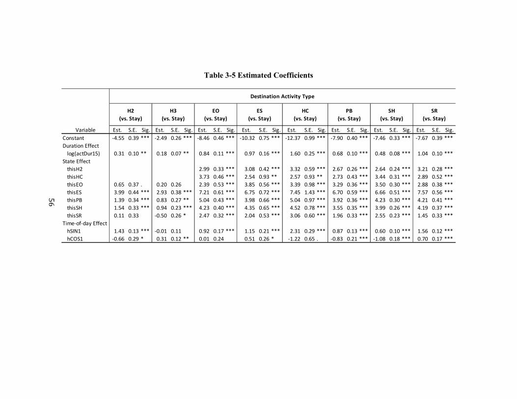
56

Table 3-5 Estimated Coefficients

Variable Est. S.E. Sig. Est. S.E. Sig. Est. S.E. Sig. Est. S.E. Sig. Est. S.E. Sig. Est. S.E. Sig. Est. S.E. Sig. Est. S.E. Sig.

Constant -4.55 0.39 *** -2.49 0.26 *** -8.46 0.46 *** -10.32 0.75 *** -12.37 0.99 *** -7.90 0.40 *** -7.46 0.33 *** -7.67 0.39 ***

Duration Effect

log(actDur15) 0.31 0.10 ** 0.18 0.07 ** 0.84 0.11 *** 0.97 0.16 *** 1.60 0.25 *** 0.68 0.10 *** 0.48 0.08 *** 1.04 0.10 ***

State Effect

thisH2 2.99 0.33 *** 3.08 0.42 *** 3.32 0.59 *** 2.67 0.26 *** 2.64 0.24 *** 3.21 0.28 ***

thisHC 3.73 0.46 *** 2.54 0.93 ** 2.57 0.93 ** 2.73 0.43 *** 3.44 0.31 *** 2.89 0.52 ***

thisEO 0.65 0.37 . 0.20 0.26 2.39 0.53 *** 3.85 0.56 *** 3.39 0.98 *** 3.29 0.36 *** 3.50 0.30 *** 2.88 0.38 ***

thisES 3.99 0.44 *** 2.93 0.38 *** 7.21 0.61 *** 6.75 0.72 *** 7.45 1.43 *** 6.70 0.59 *** 6.66 0.51 *** 7.57 0.56 ***

thisPB 1.39 0.34 *** 0.83 0.27 ** 5.04 0.43 *** 3.98 0.66 *** 5.04 0.97 *** 3.92 0.36 *** 4.23 0.30 *** 4.21 0.41 ***

thisSH 1.54 0.33 *** 0.94 0.23 *** 4.23 0.40 *** 4.35 0.65 *** 4.52 0.78 *** 3.55 0.35 *** 3.99 0.26 *** 4.19 0.37 ***

thisSR 0.11 0.33 -0.50 0.26 * 2.47 0.32 *** 2.04 0.53 *** 3.06 0.60 *** 1.96 0.33 *** 2.55 0.23 *** 1.45 0.33 ***

Time-of-day Effect

hSIN1 1.43 0.13 *** -0.01 0.11 0.92 0.17 *** 1.15 0.21 *** 2.31 0.29 *** 0.87 0.13 *** 0.60 0.10 *** 1.56 0.12 ***

hCOS1 -0.66 0.29 * 0.31 0.12 ** 0.01 0.24 0.51 0.26 * -1.22 0.65 . -0.83 0.21 *** -1.08 0.18 *** 0.70 0.17 ***

SH

(vs. Stay)

SR

(vs. Stay)

Destination Activity Type

H2

(vs. Stay)

H3

(vs. Stay)

EO

(vs. Stay)

ES

(vs. Stay)

HC

(vs. Stay)

PB

(vs. Stay)

57

3.4 Conclusion and Future Work

In this paper we explicitly proposed a hazard-based duration model in a discrete-time

framework for activity duration analysis that incorporated time dependencies into activity

episode choice and duration. We also demonstrated the fact that the discrete-time hazard-

based duration model is essentially equivalent to a discrete choice model with temporal

dummies as the simplest form of dynamic discrete choice models. In addition, we

illustrated the flexibility of the discrete-time approach by enabling complex situations of

activity-travel data to be modeled, such as multiple states of origin activity, competing

risks of destination activity, and a multilevel structure for recurrent activity episodes of

an individuals and by facilitating the integration of activity participation model with

supply model of dynamic traffic assignment (DTA).

Recently, the integration between activity-based demand models and dynamic

network supply models becomes a key issue as travel modeling research and practice

adopt the microsimulation framework. Two approaches are available for the demand-

supply integration: sequential integration and dynamic integration (Konduri, 2012). In the

traditional sequential integration approach, the demand and supply components are run

independently and sequentially in the form of an input-output data flow with a feedback

of the network conditions until convergence is achieved. The dynamic integration

approach adopts an “event-based paradigm” while constantly communicating between

the demand and supply models along a continuous time axis. In other words, the demand

model sends a set of departing trips to the supply model at every simulation minute for

those travelers who decide to move to a next activity location. The DTA supply model

58

loads these trips on the network. For those travelers who arrive at their destination, the

supply model feeds back a set of arriving trips to the demand model in every minute of

simulation. Then the demand model simulates a series of activity participation decisions,

including activity duration. As the state of practice for activity duration modeling is the

continuous-time method, we see a strong potential of the proposed discrete-time method

that can make the demand model to be dynamic or time-dependent as well. As such, in a

dynamic integration, the dynamic network model can be integrated with the dynamic

demand model with the discrete-time framework, resulting in “truly emergent” activity-

travel participation decisions.

There is a list of works we would like to pursue in our future research. First, as

mentioned previously, one important advantage of the discrete-time approach over the

continuous-time approach is the capacity to explicitly include time-varying independent

variables. To make the model more realistic, we hope to include more policy-sensitive

time-varying covariates in our model specification. For example, one can trace the

availability of household auto(s), the presence of household kid(s) at home or school, and

the jointness of other household member(s) into discrete-time intervals. Time-varying

accessibility measures, proposed in recent ABM model development, can be included as

another set of covariates to explicitly capture the temporal variation of activity

participation opportunities (Paleti et al., 2015). Second, we added the upper-level random

effects to control for unobserved individual-specific influences as well as correlation

between the unobserved individual-specific influences. Possible correlation between the

random effects was rarely detected for our population group (i.e., retirees). However, it is

59

expected to observe high correlation in random effects for other population groups, such

as workers and students. Alternative model specification with assumed correlation

structure beforehand may be better at capturing the correlation structure among these

population groups. Lastly, a potential problem with the discrete-time approach is that data

in the person-episode-period format can be extremely large, particularly when time

intervals are short and the observation period is long. One strategy to reduce the data size

is to group time intervals and then weight the grouped observations by exposure time

(Steele, Goldstein, & Browne, 2004).

60

4 MULTIPLE IMPUTATION BY CHAINED EQUATIONS

As analysis and models for land use and transportation planning gradually move to

micro-level because of policy requirements and theoretical and technical advantages

(Waddell, 2009), missing data becomes an increasingly common problem in micro-level

land use and transportation modeling and policy analysis. According to the study of

Waddell et al. (2004), up to 70% of the efforts in land use and transportation modeling

are spent on data processing, and handling missing data is a major piece of these efforts.

Missing values in land use and transportation data sets, particularly those in land

use data sets, are generally handled on an ad-hoc basis with either manual inspection and

cleaning, or rule-based or heuristic methods. While these methods can solve one type of

missing data problem at a time in some user-specified sequence, they are hard to be

adapted for different applications and there is no systematic way to assess their quality

(Waddell, 2009).

More sophisticated statistical modeling and machine learning techniques have

been developed in statistics and computer sciences and tested and applied to tackle

missing data problems in many fields such as industrial engineering (Lakshminarayan et

al., 1999), forestry (Eskelson et al., 2009), etc. Waddell (2009) suggests that k-nearest

neighbors and support vector machine may be two promising techniques for imputing

missing land use data, particularly, parcel-level data. However, to our knowledge, there is

no systematic research assessing the applicability and quality of these data imputation

techniques in imputing missing land use data.

61

Furthermore, most applications of data imputation in land use data generate a

single imputation of the missing value – that is, substitute a missing value with a single

best guess. However, single imputation masks the uncertainty in the missing values. In

other words, the imputed values in the data are treated as if they are real observed values,

without appropriately addressing the uncertainty associated with the substitutions. To this

end, Rubin (Rubin, 1987) proposes a multiple imputation framework. Instead of

producing a single best guess, multiple imputation uses a Monte Carlo simulation and

replaces each missing entry with a set of m plausible values in which m is typically small,

say 3 to 10. The advantage of multiple imputation is that, each of the m imputed data sets

can still be analyzed with standard complete-data methods, but the analysis results can be

combined by simple arithmetic calculations to produce mean estimates, standard errors,

and p-value for quantities of interest that incorporate uncertainty due to imputation of

missing data.

A popular approach to implementing multiple imputation, especially for

multivariate missing data, is multiple imputation by chained equations (MICE), also

known as fully conditional specification or sequential regression multiple imputation. It

has been widely applied in psychology (Azur et al., 2011), medicine (White et al., 2010),

epidemiology (Burgette & Reiter, 2010), etc. One of the reasons for the popularity of

MICE is its flexibility. MICE can handle missing continuous and discrete variables

because each variable with missing data is imputed based on its own imputation model.

Recent studies attempt to implement recursive partitioning within MICE in order to

62

automatically preserve interaction effects in the data (Doove et al., 2014; Shah et al.,

2014).

In this study, we apply the non-parametric MICE approach to impute missing

values in parcel data. Recently more and more land use and transportation modeling work

and analysis moves to use parcel data (Waddell, 2009). However, parcel data are prone to

problems of incomplete or missing values. In addition, in land use and transportation

modeling, base year data are usually used to project future land use and travel patterns.

So even though the number of missing values may be small, it is still necessary to impute

them. We aim to test different methods in imputing missing parcel data and assess the

quality of the imputation results, taking the uncertainty into consideration.

The remaining of this paper is organized as follows. The next section overviews

the background of missing data patterns and mechanisms, multiple imputation, MICE,

and the implementation of recursive partitioning in MICE. In the Parcel Data Imputation

section, we discuss multiple imputation for parcel data, along with missing data

description, MICE set-up, and visual diagnosis. The section that follows, we discuss the

validation of non-parametric MICE. Finally, we conclude the paper with some

suggestions for future research.

4.1 Background

4.1.1 Patterns and Mechanisms of Missing Data

For practical reasons, it is useful to distinguish three different patterns of missing data:

univariate, monotone, and arbitrary patterns (Schafer & Graham, 2002; Van Buuren,

63

2007). First, a missing data pattern is univariate if only one variable has missing values

and the remaining variables are all completely observed. For the univariate missing data,

a variety of parametric or non-parametric methods can be used for conducting multiple

imputation. Second, in the monotone pattern, more than one variable are missing and the

missing variables can be ordered such that if a variable is missing for a subject, then other

variables are also missing for that subject. Such a monotone pattern is often observed in a

longitudinal data set as one leaves the longitudinal study in the middle of entire waves of

data collection. In this case, it is possible to impute the multivariate missing data by a

series of univariate methods for multiple imputation. Lastly, an arbitrary pattern is

observed from multivariate missing variables, in which their missing values can occur in

any set of variables for any subjects. Then, we need a truly multivariate method for

multiple imputation. The arbitrary pattern is the focus of this research.

On the other hand, it is important to understand different mechanisms through

which data are missing, because different missing mechanisms may cause different risks

of bias when missing data are excluded in analysis. The missing mechanisms are

commonly classified as missing completely at random (MCAR), missing at random

(MAR), and missing not at random (MNAR). First, MCAR assumes that the probability

of data being missing depends on neither observed nor unobserved variables. In this case,

the set of subjects that are completely observed is also a random sample from the source

population. Thus, a complete case analysis in which all missing data are excluded gives

unbiased results, even if such a simple method is less efficient because the entire data set

is not used. Second, in the MAR mechanism, the probability that data are missing

64

depends on observed variables, but not on unobserved ones. In this case, a complete case

analysis is no longer based on a random sample, and selection biases are likely to occur.

Such a bias can be overcome through data imputation, in which a missing value for a

subject is replaced by a predicted value from the subject’s other known characteristics.

Lastly, a mechanism for missing data is MNAR if the probability of data being missing

depends on both observed and unobserved variables. In this case, there is no universal

method. We may only address the MNAR biases by conducting sensitivity analyses in

which the effects of different mechanisms are compared (Donders et al., 2006). As in

many other studies, the MAR mechanism is assumed in this study to apply a data

imputation approach to the missing data problems.

4.1.2 Multiple Imputation

Multiple Imputation is a statistical approach to handling missing data, which was first

proposed in the 1980s by Rubin (1987). It aims to overcome the limitation of single

imputation by allowing for the uncertainty introduced by missing data. Multiple

imputation function is increasingly available in common statistical software, such as R,

SAS, Stata, and SPSS. In general, multiple imputation consists of three steps. The first

step is to construct an imputation model, which is sometimes referred to as an imputer or

an imputation engine. For a single missing variable z, the imputer regresses z on a set of

non-missing variables among individuals with observed z values. Now each missing

value of z is replaced m times by a plausible value that is a random draw from the

predictive distribution of the imputation model.

65

The second step is usually simple. Each of the multiple imputed data sets is

analyzed separately but identically by a complete-data method (e.g., a linear regression)

to estimate quantities of interest (e.g., the regression coefficients). Since the multiple data

sets are identical for the complete data but not for the imputed data, this step generates

the m different estimates for each quantity.

The third step is to combine the m estimates, using Rubin’s rules (Rubin, 1987).

Suppose that ab< is an estimate of a scalar quantity of interest obtained from imputed data

set j (j = 1, 2, …, m) and c< is the variance of ab< . The overall estimate ab is simply the

average of the individual m estimates:

ab = 1d e ab<f

<g#

The overall variance of the overall estimate ab is formulated with two components: the

within-imputation variance (W) and the between-imputation variance (B):

h��=ab> = c + 11 + 1d2 W

The within-imputation variance explains the variation of the estimate in one imputed data

set, which is calculated by averaging the m variances:

66

c = 1d e c<f

<g#

The between-imputation variance measure how the estimates vary from imputation to

imputation to reflect the uncertainty due to missing data, which can be given:

W = 1d − 1 e(ab< − ab)$f

<g#

The greater the variation of the estimates across the imputations, the higher the

uncertainty introduced by missing data. The overall standard error is the square root of

h��=ab>. A significance test of the null hypothesis a = 0 is performed in a usual way.

Since single imputation omits the between-imputation variance, the standard error is

always too small (White et al., 2010).

4.1.3 Multiple Imputation by Chained Equations (MICE)

In large data sets with missing values such as the parcel data set, the missing values often

occur in more than one variable and follow an arbitrary pattern. When the pattern of the

multivariate missing data is arbitrary, two general multivariate approaches are available

for multiple imputation: joint modeling (JM) and multiple imputation by chained

equations (MICE). The JM approach assumes a multivariate normal distribution for all

variables in the imputation model. Imputed values are obtained from the estimated joint

67

distribution. JM was first proposed by Schafer (Schafer, 1997) and was widely used in

the earlier applications of multiple imputation to multivariate missing data. However, the

parametric method of JM may lack flexibility due to its normality assumption. In case

that there are both continuous and discrete variables, the assumption of multivariate

normality is often violated. The MICE approach is more flexible in that, instead of

assuming multivariate normality, MICE models a series of conditional distributions, one

for each missing variable, based on the other variables in the imputation model. The

semi-parametric method of MICE is increasing popular and there are many statistical

packages available for MICE (Van Buuren, 2007).

To describe the procedure of generating multiple imputed data sets in MICE,

suppose a set of variables, y1, …, yj, where some of them are missing. The following steps

are involved (Azur et al., 2011):

Step 1: Fill in every missing value by a random draw from the observed values, which

will serve as a placeholder.

Step 2: For the first missing variable, say y1, return the placeholders to missing, and

then construct an imputation model that regresses y1 on the other variables,

say y2, …, yj, only among individuals with the observed y1.

Step 3: Replace every missing value in y1 by a random draw from the posterior

predictive distribution of the imputation model for y1.

Step 4: For the second missing variable, say y2, return the placeholders to missing,

and then construct an imputation model that regresses y2 on the previously

68

imputed variable(s) y1 and the other variables y3, … yj, only among individuals

with the observed y2.

Step 5: Replace every missing value in y2 by a random draw from the posterior

predictive distribution of the imputation model for y2.

Step 6: For all other missing variables, repeat Steps 4 and 5.

Step 7: To stabilize the results, repeat Steps 2 through 6 l times (e.g., 10 to 20), which

produces one imputed data set.

Step 8: Repeat Steps 1 through 7 m times (e.g., 5 to 10) to generate m imputed data

sets.

The most significant advantage of using MICE is its ability to handle different

types of variables because each missing variable is imputed from its own imputation

model. For example, a linear regression imputer can be used to impute missing values in

a continuous variable, while a logistic regression imputation model may be constructed to

impute a discrete missing variable. When a missing variable is skewed and its

transformation to normality is impossible, Predictive Mean Matching (PMM) is usually

suggested as an imputer. PMM can be seen as a type of random k-nearest-neighbor

method (Waddell, 2009). In a PMM model, imputed values are simply sampled from the

observed values of the missing variable, so that the distribution of the imputed values is

similar to that of the observed values. Especially, PMM is desirable when the sample size

is large and a missing variable is ‘semi-continuous’ for which many values are equal

(White et al., 2010).

69

4.1.4 Recursive Partitioning in MICE

In MICE, it is required to build an imputation model for each of the variables with

missing values. In practice, however, specifying the imputation models is not an easy task

for at least two reasons. First, missing variables to be imputed may have complex

distributions. In this case, standard parametric models are not appropriate for the

imputers. Also, data transformations to normality are not always possible. Second, there

may exist interactive and nonlinear relationships among the variables in the imputers.

The nature of these interactions and nonlinearity is usually unknown a priori. It is very

laborious to add the interaction and nonlinear effects to the imputation models. To

mitigate these two challenges, recent studies suggest the use of recursive partitioning as

an imputation engine within MICE (Burgette & Reiter, 2010; Doove, Van Buuren, &

Dusseldrop, 2014; Shah et al., 2014).

One of the most popular recursive partitioning techniques is Classification And

Regression Trees (CART) (Breiman et al., 1984). CART is called either classification

trees or regression trees, depending on the response variable of interest being categorical

or continuous, respectively. In CART, a predictor space is partitioned so that

observations are clustered into several groups that are relatively homogeneous with

respect to the response variable. The best partitions are found by recursive binary splits of

the predictors. The resulting series of splits are represented in a tree structure. The leaves

of the tree represent the groups of observations, and the values in each leaf approximate

the conditional distribution of the response variable based on the predictors. Since all

splits are conditional on the previous splits, complex interactions are automatically

70

detected in the tree. The grown tree is usually pruned to avoid overfitting and for easier

interpretation. However, when a tree is built for imputation, this pruning procedure is not

desirable (Burgette & Reiter, 2010).

However, there are two major disadvantages of CART because of its hierarchical

nature. First, the trees of CART may be suboptimal. A “best” split is determined only

locally in each leaf regardless of future splits. Second, CART may produce unstable trees

because trees may vary markedly from sample to sample. In other words, small changes

in sample may lead to different initial splits and then yield quite different final trees.

Alternatively, another popular recursive portioning method is Random Forests. While

CART builds a single tree, Random Forests generates multiple trees and averages them

(Breiman, 2001). Variation in the individual trees is produced by bootstrapping and

random variable selection. Instead of using all observations, a bootstrap sample is used to

build each tree. Rather than using all variables, a subset of variables is randomly selected

to find the best split at each leaf (Doove et al., 2014).

4.2 Case Study: Parcel Data Imputation

Integrated land-use and transportation models are trending towards using disaggregated

spatial resolution, such as parcel. Although some concerns for using micro-level data

have been pointed out, such as large data requirements, long computing times, and

stochastic variations (Wegener, 2011), the advantages of using parcels as the spatial unit

of analysis are enormous. First, parcels are more behaviorally realistic in modeling the

built environment than uniform grid cells as well as coarse zones. In the real world,

71

transaction, regulation, and development usually occur at the parcel level. Second, using

the parcel geography allows us to measure walking-scale accessibility by representing

people’s activity locations on parcels. Walking access to transit stops or grocery stores

are increasingly important from public health and policy perspectives (Waddell, 2009).

In the U.S., parcel data are usually managed by local governments that assess

property taxes. There is huge variation in data completeness and data quality across

jurisdictions and missing values are common in variables that are necessary for

developing integrated models, including building square feet, building type, number of

stories, year built, building value, land value, land use, and so on. Especially for parcels

that are exempt from property taxes but nevertheless important for models, there tend to

be more missing values on the attributes. Therefore, there is a significant need for

handling missing values in parcel data as the research and practice of integrated models

move to use parcel as the spatial boundary.

For this study, we pick Multnomah County in Oregon as our study area.

Multnomah County includes Oregon’s largest city, Portland. The parcel data are obtained

from Metro’s Regional Land Information System (RLIS) that provides a variety of

geographic information for the Portland metropolitan area. Metro and the regional

partners update the parcel data every quarter. For this study we focus on one parcel data

set updated in the fourth quarter of year 2011. The parcel data set provides information

such as parcel area in square feet, building floor area in square feet, building value in

dollar, land value in dollar, land use type, and so on. We detect a modest amount of

missing entries from the parcel data set. The missing data pattern is shown in Table 1.

72

Among the total of 271,977 parcels, 83.7% are completely observed for all of the

variables. The remaining parcels have at least one missing entry for any of the variables.

The largest number of missing entries (i.e., 37,037 or 13.6%) is observed in the land-

value variable, while the smallest number of missing entries (i.e., 2,097 or 0.8%) is in the

land-use variable. Among the parcels with missing entries, 60.6% are missing for only

one variable, 37.3% for two variables, and 2.2% for three variables. We also notice that

the missing entries are scattered among the variables. Therefore, we conclude that the

missing values in the parcel data set follows an arbitrary pattern, which makes MICE a

suitable methods for imputing the multivariate missing values in the parcel data set.

Table 4-1 Missing Data Pattern of 271,977 Parcels (1 = observed & 0 = missing)

4.2.1 Setting Up MICE: Choice of Predictors

Assuming the MAR mechanism and arbitrary missing pattern, we now set up MICE to

impute all the multivariate missing values on the parcels of Multnomah County. The first

step is to determine which variables are included as predictors in the imputation models.

Table 2 is a list of the variables. We include all of the four missing variables: building

Parcel Area Land Use Building Value Building Floor Area Land Value Frequency

1 1 1 1 1 227,591

1 0 1 1 1 2,097

1 1 1 0 1 2,825

1 1 0 1 1 13

1 1 1 1 0 21,959

1 1 0 0 1 2,414

1 1 1 0 0 14,122

1 1 0 1 0 1

1 1 0 0 0 955

Total none 2,097 3,383 20,316 37,037 271,977

73

floor area, building value, land value, and land use. Since the first three continuous

variables include huge values from which it is hard to draw meaningful interpretations,

we scale down by dividing each of the three variables by parcel area. As a result, we use

three new missing variables, namely, building floor area per parcel area (i.e., FAR; floor

area ratio), building value per parcel area (i.e., BVPA), and land value per parcel area

(i.e., LVPA). It is also important to note that these three missing variables are semi-

continuous because a large portion of their values is zero and the remaining portion is

continuous. The other missing variable (i.e., LU) is categorical with 9 levels, including

agriculture, commercial, forest, industrial, multifamily residential, public/semi-public,

rural, single family residential, and vacant. Additionally, four non-missing variables are

included to increase the prediction power of the imputation models: Area, District,

POP10, and JOB11. Area is a continuous predictor, representing the parcel size in square

feet, while District is a categorical predictor with 10 polygons covering Multnomah

County among 20 districts that divide the Portland Metropolitan area for a variety of

planning and analysis purposes. The other two non-missing variables are obtained from

outside data sources. POP10 represents the 2010 population size of census block group

that the parcel belongs to, which is obtained from U.S. Census Data. JOB11 or number of

jobs in census block group that the parcel belongs to is extracted from the 2011

Workplace Area Characteristics (WAC) file of Longitudinal Employer-Household

Dynamics (LEHD). We use these two outside variables as a proxy for neighborhood

characteristics of parcels.

74

Table 4-2 A List of Predictors Included in the MICE Imputers

Variable

NameDescription

Variable

Type

Number of

Missing ParcelsMin Max Mean Median

FAR building floor area per parcel area (in square feet) semi-continuous 20,316 (7.5%) 0 4,457 1.22 0.25

BVPA building value per parcel area (in dollar) semi-continuous 3,383 (1.2%) 0 588,178 278.36 20.05

LVPA land value per parcel area (in dollar) semi-continuous 37,037 (13.6%) 0 2,232 19.42 16.47

LU 9 land use types categorical 2,097 (0.8%) - - - -

Area parcel area (in square feet) continuous no missing 2 30,956,896 35,772.12 5,433.68

Disctrict 10 districts covering Multnomah County categorical no missing - - - -

POP10 2010 population size by Census block group continuous no missing 8 4,746 1,657.36 1,407.00

JOB11 2011 number of jobs by Census block group continuous no missing 4 30,390 1,173.45 263.00

75

4.2.2 Setting Up MICE: Choice of Imputers

The aim of this study is to impute missing values in four variables, namely, FAR, BVPA,

LVPA, and LU using MICE. The key to success of a MICE application is how well the

imputation model is specified for each missing variable. In the parcel data set described

previously, missing values are observed in a mix of continuous and categorical variables

with complex distributions. Especially, three of them (i.e., FAR, BVPA, and LVPA) are

continuous but inflated with zeroes. In addition, there may exist a variety of interactions

between the predictors. For example, we can easily think of the interaction effects of land

use type and district geography on the building floor area ratio on a parcel. Multifamily

residential parcels located in CBD district tend to have a higher FAR (i.e., a higher

building on a smaller size of parcel) than the same land-use type of parcels in other

districts. Manually testing such interaction effects in the imputation model is a very time-

consuming task with no guarantee of success. For these reasons, we initially consider two

recursive partitioning methods (i.e., CART and Random Forests) as an imputation model

of MICE. We generate 5 imputed data sets (m = 5 in Step 8) after 5 iterations (l = 5 in

Step 7).

4.2.3 Visual Diagnosis

Because we never observe the missing values, we cannot quantitatively assess how well

each imputation technique performs. An important step in multiple imputation is to

diagnose whether imputations are plausible or not. As a simple visual way of checking

the plausibility of the imputations, it is useful to compare the distributions of original data

76

and imputed data. Figure 1 shows the distributions of the three continuous variables as

individual (jittered) points, in which blue points are observed data and red points are

imputed data. The zeroth imputation of all the panels contains blue points only,

representing the original distribution. The red points follow the blue points reasonably

well without showing any data points that are clearly impossible. However, it should be

noticed that the CART-based MICE did not produce proper imputes for extreme values

of FAR and BVPA. They are severely right skewed compared with LVPA; the skewness

of FAR, BVPA, and LVPA is 265, 92 and 21, respectively. For more graphical diagnostic

tools, refer to Abayomi et al. (2008). To be able to quantitatively assess the performance

of each imputation model, we will create a validation data set and compare how well each

imputation recover the true values, which will be discussed in the next section.

77

Figure 4-1 Visual Diagnosis of the CART-based MICE

78

4.3 Assessment of MICE

To evaluate the performance of MICE, we compare the predictive accuracy of the three

different MICE specifications (i.e., MICE via PMM, MICE via CART, and MICE via

Random Forests). The combination of MICE with PMM is widely used because as a

semi-parametric approach it can handle any variable types. Especially, PMM is often

used to impute a semi-continuous missing variable. It is expected that CART and

Random Forests can automatically capture complex interaction effects on missing

variables with little tuning effort needed in developing the imputation models.

To this end, we first create a validation set by removing parcels with any missing

values from the original parcel data, which produces a validation data set of 227,591

parcels with the 8 complete variables. Then, from the validation data set, we artificially

make 5 percent of the values in the four variables (i.e., FAR, BVPA, LVPA, and LU) to

be missing at random (MAR), yielding a training set of the same number of parcels but

with missing values. As shown in Table 3, the artificial missing values are evenly

scattered across all the missing variables, indicating an arbitrary pattern of missing data.

79

Table 4-3 Missing Data Pattern of 227,591 Parcels in the Training Data Set

With this training data set, we perform MICE with three different imputation

models (i.e., PMM, CART, and Random Forests). The ‘mice’ package of R is used for

the PMM-based MICE and the CART-based MICE (Van Buuren & Groothuis-

oudshoorn, 2011), while we use the ‘CALIBERrfimpute’ package of R for the MICE

imputation based on Random Forests (Shah, 2014). Each of the three MICE imputation

runs produces 5 imputed data sets as designed. It is often suggested that small numbers of

imputed data sets (e.g., 3 or 5) are sufficient unless missing rates are unusually high, say

50% (White et al, 2010). For each imputed data set, we compare the imputed values of

the training set with the original complete values of the validation set. We calculate root

mean square error (RMSE) and R-squared for the continuous variables, whereas an

accuracy rate is computed for the categorical variable (Fawcett, 2006).

Area District POP10 JOB11 FAR LVPA LU BVPA Frequency

1 1 1 1 1 1 1 1 185,350

1 1 1 1 1 1 0 1 9,745

1 1 1 1 0 1 1 1 9,711

1 1 1 1 1 1 1 0 9,883

1 1 1 1 1 0 1 1 9,729

1 1 1 1 0 1 0 1 502

1 1 1 1 1 1 0 0 532

1 1 1 1 0 1 1 0 505

1 1 1 1 1 0 0 1 512

1 1 1 1 0 0 1 1 502

1 1 1 1 1 0 1 0 516

1 1 1 1 0 1 0 0 19

1 1 1 1 0 0 0 1 33

1 1 1 1 1 0 0 0 26

1 1 1 1 0 0 1 0 26

Total none none none none 11,298 11,344 11,369 11,507 227,591

80

Table 4 shows the validation results. We find that both of the non-parametric

MICE imputations perform much better than the semi-parametric MICE for the

categorical missing variable (i.e., LU), indicated by a higher average accuracy rate for

MICE via Random Forest (0.934) and MICE via CART (0.927) than MICE via PMM

(0.780). However, it is found that there are noticeable differences in performance

between the two non-parametric imputations for the continuous missing variables. The

MICE with Random Forests performs best for LVPA; the average R-squared for LVPA is

0.450 with Random Forests, 0.426 with CART, and 0.234 with PMM. As for FAR and

BVPA, the MICE with CART performs best with the highest average R-square (0.665 for

FAR and 0.506 for BVPA). Surprisingly, the Random Forests within MICE shows a

similar performance to the PMM within MICE (0.568 and 0.569 for FAR; 0.405 and

0.406 for BVPA). The lower performance of Random Forests in this study can be

explained by a different level of skewness for the three continuous missing variables. As

mentioned earlier, as the three variables are semi-continuous, they are all severely

positive or right skewed. However, there is a significant gap in the skewness level among

the semi-continuous missing variables. The skewness of FAR, BVPA, and LVPA in the

training data set is 65, 222, and 16, respectively. The relatively high skewness, especially

of BVPA, results from some extreme data points or outliers as shown in the blue dots of

Figure 1. Since we build only 10 trees in Random Forests due to computational burden, it

is possible to easily miss the effects of such extreme values during the tree building

process of drawing bootstrap samples and selecting random input variables. Therefore,

81

we conclude that the CART-based MICE is the most appropriate for imputing missing

values in a large data set, such as the parcel data in this study.

Table 4-4 Validation Results of MICE (PMM vs. CART vs. Random Forests)

4.4 Discussion

In this paper, we have demonstrated MICE as a flexible method to implement multiple

imputation for the multivariate missing values in parcel data. We consider MICE via

PMM, and two recursive portioning techniques (i.e., CART and Random Forests) as

imputation engines for MICE. To assess their performance, we have conducted cross-

validation and found that, under limited computing power, the CART-based MICE has

m=1 m=2 m=3 m=4 m=5

RMSE 0.270 0.286 0.268 0.294 0.283 0.280

R-squred 0.590 0.558 0.586 0.547 0.565 0.569

RMSE 50.871 38.446 51.229 41.432 34.979 43.391

R-squred 0.285 0.457 0.181 0.453 0.656 0.406

RMSE 19.157 17.104 17.184 17.657 16.662 17.553

R-squred 0.179 0.250 0.236 0.232 0.276 0.234

LUAccuracy

Rate0.780 0.783 0.781 0.776 0.782 0.780

RMSE 0.247 0.222 0.248 0.238 0.238 0.239

R-squred 0.684 0.710 0.637 0.655 0.641 0.665

RMSE 43.843 34.327 30.682 34.442 45.009 37.661

R-squred 0.331 0.571 0.670 0.563 0.393 0.506

RMSE 14.484 15.269 14.306 13.801 13.955 14.363

R-squred 0.422 0.384 0.427 0.454 0.443 0.426

LUAccuracy

Rate0.927 0.925 0.930 0.924 0.928 0.927

RMSE 0.284 0.313 0.282 0.281 0.229 0.278

R-squred 0.543 0.506 0.559 0.553 0.676 0.568

RMSE 76.119 73.102 36.429 36.961 33.766 51.275

R-squred 0.195 0.187 0.541 0.515 0.585 0.405

RMSE 14.110 13.435 13.692 13.953 14.978 14.034

R-squred 0.446 0.479 0.467 0.450 0.409 0.450

LUAccuracy

Rate0.936 0.934 0.933 0.935 0.932 0.934

Average

LVPA

PMM

CART

FAR

BVPA

LVPA

Multiple Imputed Data SetImputation

Model

Missing

Variable

Validation

Measure

FAR

BVPA

Random

Forest

FAR

BVPA

LVPA

82

performed best for imputing missing values in both continuous and discrete variables,

especially when the distribution of the continuous variables to be imputed is skewed.

For future research, we plan to improve the performance of Random Forests-

based MICE by increasing the number of trees, which is expected to produce more

reliable imputers. In addition, although we have generated multiple imputed data sets, we

have not taken full advantage of them. We plan to conduct standard statistical analyses

with the resulting multiple imputed data sets and assess the uncertainty introduced via

imputed data. Lastly, this study focuses primarily on recursive partitioning methods as an

imputation model. There are many other machine learning techniques, such as k-nearest

neighbor, support vector machine, and Bayesian network that have been used in data

imputation. It would be interesting to benchmark them with the methods in this study.

83

5 CONCLUSION

Travel forecasting models have been developed to support informed decision-making

about alternative transportation and land use scenarios. The key benefit of activity-based

models is that they allow the assessment of a wider range of planning and policy than

trip-based models. Especially, activity-based models can provide significantly more

robust insights into policies and projects that may affect individuals’ activity and travel

behavior as they are implemented in a fully disaggregate microsimulation framework.

Some examples include congestion pricing, parking pricing, flexible work schedules, a

variety of transit fare policies, and so on.

However, activity-based travel forecasting is still in a formative stage. Existing

U.S. activity-based models are not fully capable of evaluating such modern transportation

and land use policies. One possible solution for having more policy-sensitivity would be

to maximize the level of details in terms of market segmentation, temporal scale and

spatial resolution, which is one of the most critical design considerations for activity-

based modeling (Castiglione et al., 2015). Unlike trip-based models, adding more

demographic segments, more time periods, and more zones does not substantially

influence run time and data storage in activity-based models. This dissertation explores

recent methodological advances to take full advantage of this key feature of activity-

based models.

First, activity-based models simulate individual households and persons in a

synthetic population. A variety of socio-demographic characteristics of residents in the

84

modeling area are used to be representative of the actual population. With all the

combinations of standard variables, thousands of different types of agents can be

considered in activity-based models, rather than just a couple of demographic segments

in trip-based models. On the other hand, individuals’ daily activity pattern is so complex

due to its multidimensionality that researchers need a method to examine the daily

patterns from a holistic point of view. Recently sequence alignment was introduced in the

field of travel behavior research to answer such an “old” question. In Chapter 2, an

innovative method was proposed by linking sequence alignment with ANODI (Analysis

of Distance). It was shown that this new methodological combination can identify unique

attributes of travelers that influence complex daily activity-travel patterns. Likewise, the

proposed method can be used to detect policy-sensitive variables for simulated

individuals. In addition, since activity-based models provide more detailed outputs with a

list of individual households, persons, tours and trips, their application for environmental

justice analysis becomes more common to understand the impacts of transportation

scenarios on different population groups (Cheng, Hu, Huang, & Wen, 2012). The

proposed method can be applied for environment justice analysis in a different way by

examining daily activity and travel patterns as a whole rather than specific accessibility

and mobility indicators.

Second, activity-based models explicitly represent time-of-day choices, such as

activity arrival and departure times as well as activity duration. Continuous-time duration

models are typically used for activity duration analysis. Chapter 3 discussed some

limitations of the continuous-time framework and proposed a discrete-time duration

85

model that is essentially a simplest form of dynamic discrete choice models. One of the

key benefits is that the discrete-time approach can easily handle time-varying constraints

and allow to track household members and cars for each of 10 or 15-min discrete-time

periods. Similarly, the most recent version of CT-RAMP explicitly traces car use at

origin and destination of each trip (Vovsha, et al., 2017). The temporal detail is critical

given that the integration of activity-based models with dynamic traffic assignment

becomes increasingly important. A strong potential of the proposed method is that the

activity-based demand model can be dynamic or time-dependent as well, so that the

integration with the dynamic supply model can result in “truly emergent” travel

forecasting.

Third, it has become more common to use multiple spatial scales in activity-based

models. For example, traffic analysis zones may be large enough for auto and transit

skimming, while microzones or parcels may reduce aggregation bias to measure

accessibilities associated with population, employment, school enrollment, parking

supply, distance to transit stops, urban density, etc. Using a smaller spatial scale is

increasingly important because transportation and land use projects pay more attention to

their local-level impacts. However, it is challenging to develop and maintain small-scale

spatial information, especially for future-year scenarios. In Chapter 3, multiple

imputation by chained equations was introduced to handle multivariate missing values in

parcel data. This sophisticate data imputation technique was adopted to develop a

continuous and reusable data hub for land use and transportation planning and modeling

(Wang & Kim, 2014).

86

As the age of Big Data has come, travel forecasting has a tremendous opportunity

to move forward to its mature status. Big Data, such as cellular tower data, navigation-

GPS data, and Location Base-Services (LBS) data, allows us to observe and understand

mobility behavior at the level of details that has never happened before (Anda, Fourie, &

Erath, 2016). Nevertheless almost all existing activity-based travel demand models rely

on conventional data sources, such as household travel surveys and census data. The

three innovative methods proposed in this dissertation may help realize the

unprecedented level of details by allowing for greater flexibility in the model

specification.

87

REFERENCES

Abayomi, K., Gelman, A., & Levy, M. (2008). Diagnostics for Multivariate Imputations.

Journal of the Royal Statistical Society: Series C (Applied Statistics), 57(3), 273-

297.

Abbott, A., & Tsay, A. (2000). Sequence Analysis and Optimal Matching Methods in

Sociology. Sociological Methods & Research, 29(3), 3-33.

Aisenbrey, S., & Fasang, A. (2010). New Life for Old Ideas: The ‘Second Wave’ of

Sequence Analysis Bringing the ‘Course’ Back Into the Life Course. Sociological

Methods & Research, 38(3), 420-462.

Anda, C., Fourie, P., & Erath, A. (2016). Transport Modelling in the Age of Big Data.

Singapore-ETH Centre.

Anderson, M. (2001). A New Method for Non-Parametric Multivariate Analysis of

Variance. Austral Ecology, 26(1), 32-46.

Azur, M., Stuart, E., Frangakis, C., & Leaf, P. (2011). Multiple Imputation by Chained

Equations: What is it and How does it Work? International Journal of Methods in

Psychiatric Research, 20(1), 40-49.

Bhat, C. (1996). A Hazard-Based Duration Model of Shopping Activity with

Nonparametric Baseline Specification and Nonparametric Control for Unobserved

Heterogeneity. Transportation Research Part B, 30(3), 189-207.

Bhat, C., & Pinjari, A. R. (2008). Duration Modeling. In D. Hensher, & K. Button (Eds.),

Handbook of Transport Modeling. Elsevier.

Bonetti, M., Piccarreta, R., & Salford, G. (2013). Parametric and Nonparametric Analysis

of Life Courses: An Application to Family Formation Patterns. Demography,

50(3), 881-902.

Bradley, M., Bowman, J., & Lawton, K. (1999). A Comparison of Sample Enumeration

and Stochastic Microsimulation for Application of Tour-Based and Activity-

Based Travel Demand Models. European Transport Conference. Cambridge, UK.

Breiman, L. (2001). Random Forests. Machine Learning, 45, 5-32.

Breiman, L., Friedman, J., Olshen, R., & Stone, C. (1984). Classification and Regression

Trees. Monterey, CA, USA: Wadsworth & Brooks.

Burgette, L. F., & Reiter, J. P. (2010). Multiple Imputation for Missing Data via

Sequential Regression Trees. American Journal of Epidemiology, 172(9), 1070-

1076.

Burnett, P., & Hanson, S. (1982). The Analysis of Travel as an Example of Complex

Human Behavior in Spatially Constrained Situations: Definition and

Measurement Issues. Transportation Research Part A, 16(2), 87-102.

Castiglione, J., Bradley, M., & Gliebe, J. (2015). Activity-Based Travel Demand Models:

A Primer. Washington D.C.: Transportation Research Board.

Cheng, H., Hu, H.-H., Huang, G., & Wen, F. (2012). Application of Activity Based

Model on Environmental Justice Analysis - a Case Study of SCAG ABM. 14th

TRB National Transportation Planning Applications Conference. Columbus,

Ohio.

88

Davidson, W., Donnelly, R., Vovsha, P., Freedman, J., Ruegg, S., Hicks, J., . . . Picado,

R. (2007). Synthesis of First Practices and Operational Research Approaches in

Activity-Based Travel Demand Modeling. Transportation Research Part A,

41(5), 464-488.

Doherty, S., & Mohammadian, A. (2011). The Validity of Using Activity Type to

Structure Tour-Based Scheduling Models. Transportation, 38(1), 45-63.

Donders, A., van der Heijden, G., Stijnen, T., & Moons, K. (2006). Review: a Gentle

Introduction to Imputation of Missing Values. Journal of Clinical Epidemiology,

59(10), 1087-1091.

Donnelly, R., Erhardt, G., Moeckel, R., & Davidson, W. (2010). NCHRP Synthesis 406 -

Advanced Practices in Travel Forecasting. Washington D.C.: Tranportation

Research Board.

Doove, L., Van Buuren, S., & Dusseldrop, E. (2014). Recursive Partitioning for Missing

Data Imputation in the Presence of Interaction Effects. Computational Statistics

and Data Analysis, 72, 92-104.

Eskelson, B., Temesgen, H., Lemay, V., Barrett, T., Crookston, N., & Hudak, A. (2009).

The Roles of Nearest Neighbor Methods in Imputing Missing Data in Forest

Inventory and Monitoring Databases. Scandinavian Journal of Forest Research,

24(3), 235-246.

Ettema, D. (1996). Activity-Based Travel Demand Modeling. PhD Dissertation.

Netherlands: Technische Universiteit Eindhoven.

Ettema, D., Borgers, A., & Timmermans, H. (1995). Competing Risk Hazard Model of

Activity Choice, Timing, Sequencing, and Duration. Transportation Research

Record: Journal of the Transportation Research Board(1493), 101-109.

Fawcett, T. (2006). An Introduction to ROC Analysis. Pattern Recognition Letters, 27(8),

861-874.

Gabadinho, A., Ritschard, G., Muller, N., & Studer, M. (2011). Analyzing and

Visualizing State Sequences in R with TraMineR. Journal of Statistical Software,

40(4), 1-37.

Gliebe, J., & Kim, K. (2010). Time-Dependent Utility in Activity and Travel Choice

Behavior. Transportation Research Record: Journal of the Transportation

Research Board(2156), 9-16.

Heckman, J., & Navarro, S. (2007). Dynamic Discrete Choice and Dynamic Treatment

Effects. Journal of Econometrics, 136(2), 341-396.

Joh, C.-H., Arentze, T., & Timmermans, H. (2001). Pattern Recognition in Complex

Activity Travel Patterns: Comparison of Euclidean Distance, Signal-Processing

Theoretical, and Multidimensional Sequence Alignment Methods. Transportation

Research Record: Journal of the Transportation Research Board(1752), 16-22.

Joh, C.-H., Arentze, T., Hofman, F., & Timmermans, H. (2002). Activity Pattern

Similarity: A Multidimensional Sequence Alignment Method. Transportation

Research Part B, 36(5), 385-403.

Kim, K. (2014). Discrepancy Analysis of Activity Sequences: What Does Explain the

Complexity of People’s Daily Activity-Travel Patterns? Transportation Research

Record: Journal of the Transportation Research Board(2413), 24-33.

89

Konduri, K. C. (2012). Integrated Model of the Urban Continuum with Dynamic Time-

dependent Activity-Travel Microsimulation: Framework, Prototype, and

Implementation.

Koppelman, F., & Pas, E. (1985). Travel-Activity Behavior in Time and Space: Methods

for Representation and Analysis. In P. Nijkamp, H. Leitner, & N. Wrigley (Eds.),

Measuring the Unmeasurable (pp. 587-627). Dordrecht, The Netherlands:

Martinus Nijhoff.

Lakshminarayan, K., Harp, S., & Samad, T. (1999). Imputation of Missing Data in

Industrial Databases. Applied Intelligence, 11(3), 259-275.

Lesnard, L. (2010). Setting Cost in Optimal Matching to Uncover Contemporaneous

Socio-Temporal Patterns. Sociological Methods & Research, 38(3), 389-419.

Martin, P., & Wiggins, R. (2011). Optimal Matching Analysis. In M. Williams, & P.

Vogt, The SAGE Handbook of Innovation in Social Research Methods (pp. 385-

408). SAGE Publications.

McArdle, B., & Anderson, M. (2001). Anderson. Fitting Multivariate Models to

Community Data: A Comment on Distance-Based Redundancy Analysis.

Ecology, 82(1), 290-297.

Paleti, R., Vovsha, P., Picado, R., Alexandr, B., Hu, H.-H., & Huang, G. (2015).

Development of Time Varying Accessibility Measures: Application to the

Activity-Based Model for Southern California. the 94th Annual Meeting of TRB.

Washington D.C.: Transportation Research Board.

Pas, E. (1983). A Flexible and Integrated Methodology for Analytical Classification of

Daily Travel-Activity Behavior. Transportation Science, 17(4), 405-429.

Pas, E. (1997). Recent Advances in Activity-Based Travel Demand Modeling. Activity-

Based Travel Forecasting Conference (pp. 79-102). Arlington: Texas

Transportation Institute.

Pinjari, A., & Bhat, C. (2011). Activity-Based Travel Demand Analysis. In A. de Palma,

R. Lindsey, E. Quinet, & R. Vickeman, A Handbook of Transport Economics (pp.

213-248). Edward Elgar Pub.

Recker, W., McNally, M., & Root, G. (1985). Travel/Activity Analysis: Pattern

Recognition, Classification, and Interpretation. Transportation Research Part A,

19(4), 279-296.

Rubin, D. (1987). Multiple Imputation for Nonresponse in Surveys. New York: John

Wiley & Sons.

Sammour, G., Bellemans, T., Vanhoof, K., Janssens, D., Kochan, B., & Wets, G. (2012).

The Usefulness of the Sequence Alignment Methods in Validating Rule-Based

Activity-Based Forecasting Models. Transportation, 39(4), 773-789.

Saneinejad, S., & Roorda, M. (2009). Application of Sequence Alignment Methods in

Clustering and Analysis of Routine Weekly Activity Schedules. Transportation

Letters: The International Journal of Transportation Research, 1(3), 197-211.

Schafer, J. (1997). Analysis of Incomplete Multivariate Data. London, United Kingdon:

Chapman & Hall Ltd.

Schafer, J., & Graham, J. (2002). Missing Data: Our View of the State of the Art.

Psychological Methods, 7(2), 147-177.

90

Schlich, R., & Axhausen, K. (2003). Habitual Travel Behaviour: Evidence from a Six-

Week Travel Diary. Transportation, 20(1), 13-36.

Shah, A. (2014). CALIBERrfimpute: Imputation in MICE using Random Forest.

Retrieved from http://cran.r-

project.org/web/packages/CALIBERrfimpute/index.html

Shah, A., Bartlett, J., Carpenter, J., Nicholas, O., & Hemingway, H. (2014). Comparison

of Random Forest and Parametric Imputation Models for Imputing Missing Data

Using MICE: a CALIBER Study. American Journal of Epidemiology, 179(6),

764-774.

Shoval, N., & Isaacson, M. (2007). Sequence Alignment as a Method for Human Activity

Analysis in Space and Time. Annals of the Association of American Geographers,

97(2), 282-297.

Singer, J., & Willett, J. (2003). Applied Longitudinal Data Analysis: Modeling Change

and Event Occurrence. New York: Oxford University Press.

Steele, F. (2005). Event History Analysis. Bristol: ESRC National Centre for Research

Methods.

Steele, F. (2008). Multilevel Models for Longitudinal Data. Journal of the Royal

Statistical Society: Series A (Statistics in Society), 4(2), 5-19.

Steele, F. (2011). Multilevel Discrete-Time Event History Models with Applications to

the Analysis of Recurrent Employment Transitions. Australian and New Zealand

Journal of Statistics, 53(1), 1-26.

Steele, F., Diamond, I., & Wang, D. (1996). The Determinants of the Duration of

Contraceptive Use in China: A Multi-level Multinomial Discrete-Hazards

Modeling Approach. Demography, 33(1), 12-23.

Steele, F., Goldstein, H., & Browne, W. (2004). A General Multilevel Multistate

Competing Risks Model for Event History Data, with an Application to a Study of

Contraceptive Use Dynamics. Statistical Modelling, 4(2), 145-159.

Studer, M., Ritschard, G., Gabadinho, A., & Müller, N. (2011). Discrepancy Analysis of

State Sequences. Sociological Methods & Research, 40(3), 471-510.

Van Buuren, S. (2007). Multiple Imputation of Discrete and Continuous Data by Fully

Conditional Specification. Statistical Methods in Medical Research, 16(3), 219-

242.

Van Buuren, S., & Groothuis-oudshoorn, K. (2011). mice : Multivariate Imputation by

Chained Equations in R. Journal of Statistical Software, 45(3).

Vovsha, P., & Bradley, M. (2004). A Hybrid Discrete Choice Departure Time and

Duration Model for Scheduling Tours. Transportation Research Record: Journal

of the Transportation Research Board(1894), 46-56.

Vovsha, P., Bradley, M., & Bowman, J. (2005). Activity-Based Travel Forecasting

Models in the United States: Progress since 1995 and Prospects for the Future. In

H. Timmermans (Ed.), Progress in Activity-Based Analysis (pp. 389-414).

Amsterdam, the Netherlands: Elsevier.

Vovsha, P., Hicks, J., Vyas, G., Livshits, V., Jeon, K., Anderson, R., & Giaimo, G.

(2017). Combinatorial Tour Mode Choice. 96th Annual Meeting of the

Transportation Research Board. Washington D.C.

91

Waddell, P. (2009). Parcel-Level Microsimulation of Land Use and Transportation: The

Walking Scale of Urban Sustainability. Resource Paper for the 2009 IATBR

Workshop.

Waddell, P., Peak, C., & Caballero, P. (2004). UrbanSim: Database Development for the

Puget Sound Region. Seattle: Center for Urban Simulation and Policy Analysis,

University of Washington.

Wang, L., & Kim, K. (2014). Continuous Data Integration for Land Use and

Transportation Planning and Modeling. National Institue for Transportation and

Communities.

Wegener, M. (2011). From Macro to Micro – How Much Micro is too Much? Transport

Reveiws, 31(2), 161-177.

White, I., Royston, P., & Wood, A. (2010). Multiple Imputation Using Chained

Equations: Issues and Guidance for Practice. Statistics in Medicine, 30(4), 377-

399.

Wilson, C. (1998). Analysis of Travel Behavior Using Sequence Alignment Methods.

Transportation Research Record: Journal of the Transportation Research

Board(1645), 52-59.

Wilson, C. (2001). Activity Patterns of Canadian Women: Application of ClustalG

Sequence Alignment Software. Transportation Research Record: the Journal of

the Transportation Research board, 1777, 55-67.

Wilson, C. (2008). Activity Patterns in Space and Time: Calculating Representative

Hagerstrand Trajectories. Transportation, 35(4), 485-499.