Embed Size (px)
Citation preview

Real-‐&me Simula&on and Preventa&ve Control of Power Blackouts
Shrirang Abhyankar Computa(onal Engineer Center for Energy, Environment, and Economic System Analysis (CEEESA) Energy Systems Division [email protected] hAp://www.mcs.anl.gov/~abhyshr

Focus on LARGE Power Blackouts
2003 Northeast Blackout affected 55 million people

LARGE Power Blackouts
Southwest Blackout 2011 affected 7 million people

LARGE Power Blackouts
India Blackout 2012 affected 600 million people

Blackouts are bad

Blackouts are bad

especially when it interrupts a SuperBowl game
P2S2 Workshop Panel (09/10/2012)
Aerial view of the San Diego stadium during the third quarter of the Superbowl Game 2012

Causes of Power Blackouts

Causes of Power Blackouts

Favorable condi&ons for blackout
Genera&on-‐Load Imbalance Abnormal voltages

Power System Simula&on Research Thrust Areas
§ Parallel Extensible Toolkit for Power System Simula(on (PETPSS)
§ Simula(on of Power blackouts – Modeling and solver difficul(es – Achieving Real-‐Time or Faster-‐than-‐Real-‐Time Simula(on Speed.
– Preventa(ve control

Parallel Extensible Toolkit for Power System Simula&on (PETPSS)
Algorithms, Solvers Math and Computa&onal Layer
(PETSc)
Power System Layer Models, Toplogy
Applica&on Layer Applica&on Interface
Power Flow
Dynamics
Op(mal Power Flow
Con(ngency Analysis
Dynamics Constrained Op&mal Power Flow
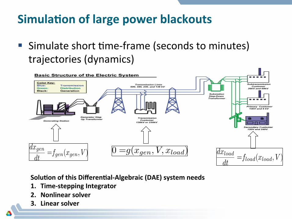
Simula&on of large power blackouts
§ Simulate short (me-‐frame (seconds to minutes) trajectories (dynamics)
dxgen
dt
=fgen(xgen, V ) 0 =g(xgen
, V, x
load
)dx
load
dt
=f
load
(xload
, V )
Solu&on of this Differen&al-‐Algebraic (DAE) system needs 1. Time-‐stepping Integrator 2. Nonlinear solver 3. Linear solver

Modeling and Solver Difficul&es 2003 Blackout Precursor events
12:15pm 1:31pm 2:02pm 3:05pm 3:17pm
State es(mator Failure
Genera(ng plant Shuts down
Several major Transmission lines Out due contact With tree
Major Line outage due to contact with tree
Major Transmission line Out due contact With tree
3:41pm
Protec(on trips a major line causing 15 other lines to fail
4:05pm
Major transmission Line tripped due to Undervoltage and Overcurrent condi(ons

Modeling and Solver Difficul&es Capturing dominos as they fall

Modeling and Solver Difficul&es
2003 NE Blackout Simula&on Simulated versus Recorded

Modeling and Solver Difficul&es 48
0 0.05 0.1 0.15 0.2 0.25 0.3 0.35 0.4 0.450.6
0.65
0.7
0.75
0.8
0.85
0.9
0.95
1
1.05
Time(sec)
Voltage Magnitude(pu)
Generator Terminal
Load Bus
Figure 5.8 Voltage magnitude plot for line tripping at dP = 2.32 pu
0 0.05 0.1 0.15 0.2 0.25 0.3 0.35 0.4 0.45376.94
376.95
376.96
376.97
376.98
376.99
377
Time(sec)
Generator Speed(rad/sec)
Figure 5.9 Generator speed plot for line tripping at dP = 2.32 pu
No Solution???
No Solution???
Is this leading to a blackout?

Allevia&ng solver difficul&es 72
0 0.05 0.1 0.15 0.2 0.25 0.3 0.35 0.4 0.450
0.2
0.4
0.6
0.8
1
1.2
1.4
Time(sec)
Volta
ge m
agnit
ude(
pu)
Generator TerminalLoad Bus
Figure 5.40 Collapse of load bus voltage captured in transient stability simulations using voltage dependent impedance load model.
0 0.05 0.1 0.15 0.2 0.25 0.3 0.35 0.4 0.45-200
-150
-100
-50
0
50
100
150
Time(sec)
Phas
e An
gle(d
eg)
Generator TerminalLoad Bus
Figure 5.41 Phase angle oscillations at the load bus
Pn = P0
✓Vn
Vn�s
◆2
Improved load modeling
Voltage collapse trajectory

Real-‐&me Blackout simula&ons
§ What’s the need? – Assist operators to assess dynamics in real-‐(me when events are evolving.
§ Issue: Such simula(ons are too slow (not real-‐&me speed)
Transmission system control center

Achieving Real-‐Time Dynamic Simula&on Speed: 1. Paralleliza&on
Single processor
G
G
G
G
Vec
Two processors
G
G Vec
G
G Vec
Communica(on
P0 P1
Mul&ple processors (cores) used for solving the problem

Achieving Real-‐Time Dynamic Simula&on Speed: 2. Efficient parallel linear solvers
Linear solver is the biggest computa&onal boXleneck!!
Time Integra&on
Nonlinear Solve
Linear Solve Nonlinear solver
Parallel linear solver achieved 10X linear solver speedup on 16 cores for a 50,000 bus test system
Execu(on (me

Achieving Real-‐Time Dynamic Simula&on Speed: 3. Adap&ve Time-‐stepping
44
With the continuation power flow as the basis for the transient stability studies,
the transient stability simulations were carried out by tripping branch 4-5 at 0.2 seconds.
The basic aim of the transient stability simulations was to determine whether the system
can survive the transient and reach the corresponding steady state operating point on the
PV curve with one line in service. The line tripping was modeled by taking out branches
1-4, 4-5 and 5-6. The load was assumed to hold its constant PQ characteristic throughout
the transient. The response of the system to line tripping at various loading levels is
described in the following sections.
5.2.1 Loading upto 2.31 pu. The first simulation involved the transient analysis of the
system for a loading level of dP = 1.0 pu. The response of the system to tripping a line is
shown in Figures 5.4 -5-5.
0 5 10 15 20 250.93
0.94
0.95
0.96
0.97
0.98
0.99
1
1.01
Time(sec)
Voltage M
agnitude
(pu)
Generator TerminalLoad Bus
Figure 5.4 Voltage magnitude plot for line tripping at dP = 1.0 pu
Take smaller steps when things are evolving rapidly, larger steps otherwise
�t �t �t
�tn+1 = �tn||en+1||�1/p
Time-‐step adap&vity

0.00
1.00
2.00
3.00
4.00
5.00
6.00
7.00
1 2 4 8 16 24
Execu&
on &me (sec)
# Cores
Achieving Real-‐Time Dynamic Simula&on Speed: Puang it all together: Test case 1
Faster-‐than-‐real-‐&me
Slower-‐than-‐real-‐&me
Scalability plot of a 5 second simula&on of a 20,000 node system
-‐ Achieved faster-‐than-‐real-‐&me speed of under 1 second execu&on &me on 16 cores.
-‐ Execu&on &me using state-‐of-‐the-‐art algorithm on single core = 35 seconds
0
5
10
15
20
1 2 4 8 12
Execu&
on Tim
e (sec)
#cores
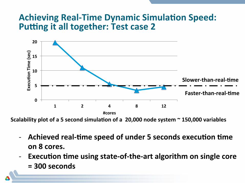
Achieving Real-‐Time Dynamic Simula&on Speed: Puang it all together: Test case 2
Faster-‐than-‐real-‐&me
Slower-‐than-‐real-‐&me
Scalability plot of a 5 second simula&on of a 20,000 node system ~ 150,000 variables
-‐ Achieved real-‐&me speed of under 5 seconds execu&on &me on 8 cores.
-‐ Execu&on &me using state-‐of-‐the-‐art algorithm on single core = 300 seconds

Preventa&ve control of Power Blackouts: The Gotham Analogy
h
JOKER’S NO FLY ZONE

Preventa&ve control of Power Blackouts: The Gotham Analogy
h
You need to re&re Alfred

Preventa&ve control of Power Blackouts: The Gotham Analogy
h
Thank you Mr. Fox!

Preventa&ve Control of Power Blackouts
§ Modify ini(al opera(ng point by including scenarios that could violate security and poten&ally lead to blackouts.
§ Need to solve an “Op(mal Control” problem
28
Op(mal Power Flow
(Nonlinear Op&miza&on)
Transient Stability (Differen&al-‐
Algebraic Equa&ons)
min C(p)
s.t. gs(p) = 0
hs(p) h+
p� p p+
x = f(x, y, p), x(t0) = I
x0(p)
0 = g(x, y, p), y(t0) = I
y0(p)
h(x(t), y(t)) 0, 8(t)
� =� fT
x
�+ gTx
µ� hx
0 =� fT
y
�+ gTy
µ� hy
rpH =
Z T
0fTp � dt �
�xTp �
����t=0
p
Path constraints
Adjoint-‐sensi(vity based gradient calcula(on

Preventa&ve Control of Blackouts
Generator 3 would trip
Without incorpora&ng dynamic scenarios
Modified dispatch by incorpora&ng both scenarios
On-going work and future steps
I Optimization with multiple dynamics scenarios (faults atdi↵erent locations).
Total cost = $6216.08Generator Bus Number MW
Gen1 1 162.71Gen2 2 103.16Gen3 3 51.53
0 0.5 1 1.5 2 2.5 358.5
59
59.5
60
60.5
61
61.5
Time (sec)
Fre
qu
ency
= ω
/2π
Figure: Generator frequencies forfaults at Bus 7 and Bus 9
I Low-level implementation (PETSc + IPOPT)I Mixed-BFGS approach for computing HessianI Parallelizing dynamics scenariosI Transiently unstable scenarios
Without dynamic constraints
Total cost = $5297.41
Table: Generation schedule without dynamic constraints
Generator Bus Number MW
Gen1 1 89.81Gen2 2 134.33Gen3 3 94.20
0 0.2 0.4 0.6 0.8 158.5
59
59.5
60
60.5
61
61.5
Time (sec)
Freq
uenc
y =
ω/2
π
Gen 1
Gen 2
Gen 3
Figure: Generator frequencies forfault at Bus 7
0 0.2 0.4 0.6 0.8 158.5
59
59.5
60
60.5
61
61.5
62
Time (sec)
Freq
uenc
y =
ω/2
π
Gen 1
Gen 2
Gen 3
Figure: Generator frequencies forfault at Bus 9
Generator 2 would trip

Summary
§ Presented relevant research on modeling, real-‐(me simula(on, and preven(ve control of large power blackouts.
§ We are off to a promising start, but there’s s(ll a long way to go.

QUESTIONS??


