DOI: 10.20357/B7TS3G

Realizing high-accuracy low-cost measurement and verification for deep cost savings

Jessica Granderson, Samir Touzani, Eliot Crowe, Samuel Fernandes, Shankar Earni, Kaiyu Sun

Building Technology and Urban Systems Division Lawrence Berkeley National Laboratory

Energy Technologies Area September 2019

Final Project Report

Prepared for: Todd Amundson Bonneville Power Administration

Disclaimer: This document was prepared as an account of work sponsored by the United States Government. While this document is believed to contain correct information, neither the United States Government nor any agency thereof, nor the Regents of the University of California, nor any of their employees, makes any warranty, express or implied, or assumes any legal responsibility for the accuracy, completeness, or usefulness of any information, apparatus, product, or process disclosed, or represents that its use would not infringe privately owned rights. Reference herein to any specific commercial product, process, or service by its trade name, trademark, manufacturer, or otherwise, does not necessarily constitute or imply its endorsement, recommendation, or favoring by the United States Government or any agency thereof, or the Regents of the University of California. The views and opinions of authors expressed herein do not necessarily state or reflect those of the United States Government or any agency thereof or the Regents of the University of California.

1

This report comprises Lawrence Berkeley National Laboratory’s final deliverable under the BPA Technology Innovation (TI) Project “Realizing high-accuracy low-cost measurement and verification for deep cost savings.”

1. Introduction

The project “Realizing high-accuracy low-cost measurement and verification for deep cost savings”, that began in Fiscal Year (FY) 2017, was funded to conduct the technical analyses, demonstration, market evaluation, and regulatory engagement necessary to realize a cost-effective high-accuracy advanced measurement and verification (M&V) method that could be applied to certain efficiency programs in the Pacific Northwest. Advanced M&V (also known as M&V 2.0), is a method that uses advanced metering infrastructure (AMI) data in combination with analytics to quantify energy efficiency savings. The foundation of the advanced M&V methods utilized under this project was whole-building M&V for commercial buildings, as defined in Option C of the International Performance Measurement and Verification Protocol (IPMVP) (EVO 2012). The goal of the project was to address unanswered questions about the use of Advanced M&V such as: How accurately can these tools be applied to quantify efficiency project savings? How can advanced M&V be used to satisfy regulatory requirements for rigorous savings estimates? Building upon prior work by Lawrence Berkeley National Laboratory (Berkeley Lab) and others that have tested the accuracy of proprietary and open-source Option C baseline models (Granderson 2015a, 2015b, 2016), the key objectives of this project were to:

• Develop practitioner workflows that integrate advanced M&V tools with supplementary automated routines for non-routine adjustments and for quantification of savings uncertainty to indicate rigor.

• Demonstrate these workflows with Seattle City Light, in collaboration with their implementers and evaluators – determine labor and time/cost savings, and uncertainty of the results obtained.

• Engage the Pacific Northwest regulatory community to determine acceptance criteria for the required accuracy and reporting of advanced whole-building M&V.

• Document the findings to facilitate broad industry uptake of the solutions. This project directly supports the R&D Programs and Research Questions specified in the Technology Area “Low-cost Saving Verification Techniques,” in Volume 6 (Sensors, Meters, and Energy Management Systems) of the BPA Technology Roadmaps1. The work provided several of the outcomes targeted in R&D Program Whole-building Regression Analysis Validation (p.33); it also included key questions noted in Acceptable M&V (p.29), and Measuring and Using Independent Variables (p.39).

1 https://www.bpa.gov/EE/Technology/EE-emerging-technologies/Documents/EE_Tech_RM_Portfolio.pdf

2

To date, this work has resulted in three peer-reviewed publications (Crowe 2019; Granderson 2017; Touzani 2019), public open source availability of a non-routine event detection algorithm via the RM&V2.0 tool2, and public dissemination of findings from the advanced M&V pilot through conferences and industry presentations. The work on non-routine event detection under this project is being extended through research sponsored by the U.S. Department of Energy. This report is divided into seven sections, with each section summarizing results from different tasks of the project. Section 2 provides an overview of the literature and market review, section 3 provides an overview of the non-routine adjustment task, section 4 on uncertainty quantification, section 5 the practitioner workflows, section 6 regulatory engagement, section 7 the Seattle City Light demonstration and finally section 8 includes a discussion and conclusion section with a summary of the overall findings from this project.

2. Literature and market review

The purpose of the literature and market review was to summarize the current state of the industry with respect to M&V tool capabilities, and document interest from state energy agencies and utilities to implement advanced M&V processes. This review was designed to provide BPA, Seattle City Light, and other Pacific Northwest stakeholders a summary of what program activity was currently being implemented in the rapidly changing landscape surrounding M&V tools and associated program applications. The resulting information was also used to inform subsequent activities undertaken in the project. Published in (Granderson 2017), the literature and market review comprised characterization of 16 commercially available advanced M&V technologies combined with a summary of how they are being used nationally in utility programs. The technology characterization was based on a framework of twelve characteristic elements including target market and user, principal design intent, M&V methods and mathematical approach, model fitness and uncertainty capabilities, and user-adjustable parameters. Key conclusions regarding the state of technology and its application in industry are excerpted in the following paragraphs. Commercial building sector applications are targeted by advanced M&V 2.0 tools more often than residential and industrial sectors. When current advanced M&V tool features are compared to prior published findings (Kramer 2013) several changes in technology capabilities can be identified. Many tool providers now identify M&V as a core element of their principal design intent, and there has been an increase in the number of offerings that accommodate both monthly and interval data. There is also an increase in the number of solutions that offer isolation-based Option B savings analysis as well as whole-building level Option C analyses (however it may be that approaches other than whole-building were either not addressed in this prior work, or were intentionally not included). There is also indication that R2 and CV(RMSE) are emerging as common model fitness metrics, providing insight into savings uncertainty. Although not explicitly covered in prior published work, discussion with vendors suggested that they are beginning to explore more advanced modeling techniques such as non-linear and machine learning approaches. 2 https://github.com/berkeley lab-eta/rmv2.0

3

It is worth noting several important ways in which the market has not changed, for example:

• There remain a relatively small number of tools that offer savings estimation based on Option D calibrated simulation modeling. This is related to the fact that the majority of the technologies surveyed are used for meter data analysis and visualization for operational efficiency—it is still the case that data-driven techniques dominate the tools used for continuous operational analyses, while simulation-based methods are primarily used in design and retrofit analysis.

• There is still a need for comprehensive solutions to identify, verify, and address non-routine adjustments.

• Although transparency is still a common part of industry dialogue, about half of vendors surveyed in prior work and today report a strong willingness not to disclose model equations and specifications.

In terms of regulatory and programmatic policy development around advanced M&V there has been significant activity over the past decade, though there are no examples to date of widespread adoption. Notable examples of recent efforts include:

• California, Senate Bill (SB) 350 and Assembly Bill (AB) 802 establish aggressive goals to increase building energy efficiency, and permit tracking and incentivizing savings through meter-based and pay-for-performance approaches. The California Public Utility Commission (CPUC) has established guidelines for advanced M&V (known as “Normalized Metered Energy Consumption” methods), and a limited initial round of programs is ramping up.

• The Northeast Energy Efficiency Partnerships’ EM&V Forum has initiated a multi-year dialogue with its members on the opportunities and limitations of M&V 2.0 in the context of the northeast regulatory and program delivery and evaluation context. NEEP is also supporting an advanced M&V pilot in Connecticut, along with regulators, utilities, and Berkeley Lab.

• For several years the Consortium for Energy Efficiency’s (CEE’s) Whole Building Committee has focused on supporting members to understand the opportunities for whole-building focused program delivery, including design considerations as well as whole-building level M&V, and the role of M&V 2.0 in implementation and evaluation.

These and other national efforts are complementary to BPA’s work in the Pacific Northwest (referenced in Section 6) to establish technical guidance and program approaches (notably, Strategic Energy Management). The level of national activity in M&V 2.0 and associated whole-building, operational, behavioral, and maintenance programs indicates a high level of interest. However, it is important to recognize that the industry is still grappling with several issues related to M&V 2.0’s usefulness and ultimate value. In 2017 the authors convened a national M&V 2.0 stakeholder group comprising a cross section of subject matter experts from the program administration, evaluation, implementation, and regulatory communities, as well as from the M&V 2.0 vendor community. The group was asked to identify the critical needs for industry with respect to M&V 2.0. Resonating with recent literature (Franconi 2017), five topics were ranked most highly:

4

1. Pilots to demonstrate the practical viability of M&V 2.0 2. Standard requirements for accuracy and reporting of M&V 2.0 results 3. Methods to handle non-routine events and adjustments 4. Standard M&V 2.0 software testing procedures 5. Expansion of the methods in today’s tools to handle baselines other than existing conditions

The first three of these topics were further addressed in the broader TI project; results are presented in sections 3, 5, and 7 of this report.

3. Non-routine event detection and adjustment

In advanced M&V applications, non-routine events (NREs) cause changes in building energy use that are not attributable to changes in the independent variables used in a baseline model, or to the efficiency measures that were installed. The ability to detect and adjust for non-routine events is important for ensuring that reported savings are indeed those attributable to the installed measures. Correspondingly, the project team explored the development of standard methods to identify and quantify commonly encountered non-routine events. Three analytical methods were investigated – one based on statistical time series change detection, one based on Energy Plus simulation modeling, and the other based on the use of Energy Star’s Portfolio Manager regressions. Each of these methods is described below.

3.1 Statistical time series change detection

In this approach, a data-driven methodology was developed to partially automate the process of detecting NREs in the post-retrofit period. The algorithm developed was based on the PELT statistical change point detection method (Killick 2014). Change points are considered to be the locations in a time series where a change in the statistical properties of the sequence of observations is observed. The change-point NRE detector was integrated into the Berkeley Lab open source RM&V2.03 tool for visual testing and validation, and for further empirical testing and validation using actual project data. Figure 1 shows a screen shot of the detector applied to project data for two sites. Changes in the y-value of the horizontal red line indicate a detected change in the post-period energy consumption time series, and therefore a potential NRE. The results of the NRE detector were reviewed in conjunction with cumulative savings (CUSUM) plots (Example in Figure 2), as a diagnostic for NRE identification in the demonstration with Seattle City Light that is described in section 7.

3 The term “RM&V” is the name of Berkeley Lab’s open source tool, and is not an acronym in general use. The name is derived from the fact that the tool was built using the R statistical software package.

5

Figure 1: Screenshot from open-source RM&V2.0 tool, illustrating the output of the NRE detection algorithm

Figure 2: Example CUSUM chart, indicating potential NREs Following development of the NRE detection algorithm and its integration into the RM&V2.0 tool, funding from the U.S. Department of Energy was used for additional testing and development. Documented in Touzani 2019, two enhanced detection options were also explored. These enhanced detectors used a ‘dissimilarity metric’ in addition to the PELT changepoint algorithm. The dissimilarity metric measures the proximity between the actual post-retrofit energy consumption and the projected baseline (which is generated using a statistical baseline model, and used as the counterfactual in the savings estimate). In addition to the enhanced NRE detectors, Touzani 2019 describes and tests a semi-automated methodology to quantify the savings impact of NREs, once an NRE has been confirmed to be present. That non-routine adjustment (NRA) methodology comprises six steps: (1) estimate the start date and duration of potential NREs using the NRE detection algorithm; (2) verify which detected NREs merit an adjustment to the saving calculation using project information or site inquiry, and validate their actual date of occurrence; (3) exclude from the reporting period time

Step change in red line indicates date of possible NRE

Major changes in direction of CUSUM curve suggest possible NREs

6

series the data points from the verified NRE periods; (4) train a regression model using the remaining data of the post period time series; (5) use the trained model to predict what the energy consumption would have been within the NRE periods if no NRE was present; (6) use the model-predicted values as replacement data for the periods in which the NRE was present. The final step of the methodology produces the adjusted time series for the whole reporting period. The three NRE detection algorithms, and the NRA methodology were tested using simulated scenarios representing a diversity of NRE types, and the time series energy consumption data that was output from the simulations. Key conclusions were:

• The performance of the detection portion of one of the enhanced algorithms was quite strong, both in an absolute sense, and versus the two other tested algorithms, with a true positive rate ranging from 75%-100%.

• The false positive NRE detection rate was lower for one of the enhanced algorithms in the majority of test cases, however, with a range of 20%-70% is likely higher than ideal.

• The NRA results that were presented showed 0.7% error or less in the final energy savings estimates, versus (simulated) ground truth, once adjustments were made to account for the non-routine events.

o This represents a best-case scenario for which the event dates are known with certainty.

o In real-world application, there will likely be some uncertainty in isolating precise dates of event occurrence.

The results showed that the proposed approach holds promise for helping M&V practitioners streamline the process of detecting NREs and adjusting the corresponding energy consumption to improve the accuracy of the meter-based savings estimates. There are many opportunities for future research, beginning with testing and validation against a larger set of simulated scenarios, and testing against data from real buildings and projects. Further work is needed to explore the impact on algorithm performance of parameters such as NRE duration, magnitude and type, and building type. Use by practitioners will provide valuable insights as to the practical viability of the approach, and suitability of the current balance between true and false positive rates.

3.2 Non-routine adjustments based on regression and simulation modeling

3.2.1 Regression modeling

In addition to the changepoint-based approaches to handling non-routine events, the use of Energy Star Portfolio Manager (ESPM) was also explored. The objective of this project task was to explore whether the ESPM regression models could be used to develop a simple calculator for NRA estimates. The logic behind the approach is that ESPM models show how energy consumption changes with changes in key variables such as occupancy, operating hours, etc.4, and some of these

4 Variables such as occupancy, operating hours, etc., are treated as “static factors” when energy modeling is based on ambient temperature alone, i.e., factors that are assumed to be unchanged from the baseline period to the reporting period.

7

key variables are aligned with common NREs. Hence, perhaps the ESPM models could be used to come up with a set of standardized adjustment factors for certain commonly encountered NREs. ESPM normalizes building energy consumption to account for differences in buildings’ physical characteristics, operating conditions and activities using a regression model. The regression model is developed based on underlying CBECS data to understand aspects of building activity, operations or characteristics that are statistically significant with respect to energy use. This linear regression is used to estimate the building’s source energy use intensity as a function of several variables (Xi) such as occupancy level, number of computers, etc. (also called independent variables). C0 represents a constant term and the other Ci values are regression coefficients.

Y=C0+ C1X1+C2X2+C3X3+…CnXn

It is important to note that, in order to assess the impact of a factor on change in energy consumption, only information related to the old and new values of the effect factor are needed, assuming all the other factors remain the same and will not affect the energy consumption. In the following we provide an example for a non routine adjustment to account for a change in weekly operating hours for a regular office building.

a. Identify the ESPM regression model for the building type of interest. which of the ESPM building types characterizes the building type for which net effect of a static factor or factors are being estimated

The source EUI for an office building can be predicted by: y ̂ =186.6 + 34.17ln(X1) + 17.28(X2) + 55.96ln(X3) + 10.34ln(X4) +0.0077(X5)(X6) + 0.0144(X7)(X8) -64.83(X9)ln(X1) +34.20(X9)ln(X4) +56.30(X9)

Where X1 is area of the office building in square footage, X2 is the number of computers per 1000 square feet, X3 is weekly operating hours, X4 is the number of workers per 1000 square feet, X5 is the heating degree days, X6 is percentage of the building that’s heated, X7 is the cooling degree days, X8 is percentage of the building that’s cooled, X9 represents binary value indicating whether the office building is a small bank.

b. Identify the independent variable or variables in the regression model that characterize the non-routine events being quantified, and quantify the net impact of the static factor changes on the source EUI using the relevant part of the equation described by ESPM

Part of the equation to study the effects of changes to weekly occupancy hours (X3)

y = 55.96[(X3)-(X’3)] Where y is the change in source EUI, X3 and X'3 is the weekly operating hours before and after the non-routine change.

8

c. Convert the source EUI difference to actual difference in site energy consumption for the

entire building. z = (y)*(X1)/K

Where z is the net change in buildings energy consumption due to a change in given static factors, K is source to site ratio, X1 is area of the building in square footage.

d. If the change in the static factor lasted for less than year, the annual effect needs to be

prorated appropriately to ensure proper accounting for this change. The approach that was illustrated in this example could be applied in the same manner, for different building types and non-routine event types, so long as they are represented in the ESPM regressions. The strengths and limitations of this approach are:

• This approach can be applied to a large number of building types and potential NRE types that align with the independent variables in the ESPM regression models.

• The regression models defined by ESPM are fairly well accepted by the buildings’ energy efficiency community.

• It is difficult to quantify the effect of NREs that are sustained for a partial year, especially if the impact is nonlinear.

• The approach represents the mean energy use for a group of ‘typical’ buildings with the same characteristics; it is not able to account for the specific baseline energy consumption of the building whose energy use/savings are being adjusted.

3.2.2 Simulation modeling

In order to evaluate the results from the ESPM model and study its suitability to predict the effect of static factors on energy consumption, an alternate approach using EnergyPlus simulations was developed. The simulations served as a check on the results of the ESPM approach, and also provided an alternative method to determine NRAs. A number of simulations using the DOE reference office model were conducted to assess the impact of static factors studied using the ESPM model. These static factors were workers/computers and hours of occupancy, which were modeled in the range of -30% to +30%. In addition to the static factors, other parameters were varied including orientation, envelope, thermostat settings, infiltration and HVAC efficiencies. The results from the metamodel based simulation approach are compared with the ESPM regression approach (Figure 3 & 4). From these initial results for an office building, the ESPM approach to assess the impact of the given static factors (workers/computers and hours of occupancy) is producing results that are similar to the more detailed simulation results for a given building. However, it is important to note that the simplified ESPM model results are based on national averages using underlying CBECS data that does not take into account a specific building’s characteristics and its baseline energy consumption or performance. Further, the estimated impact of parameter changes on EUI using this model is an average for all buildings, hence not associated with the conditions of the investigated building.

9

Figure 3: Plot showing the average % change in EUI for large office buildings for change in workers/PCs based on ESPM model and model based on simulation results

Figure 4: Plot showing the average % change in EUI for large office buildings for change in hours of operation based on ESPM model and model based on simulation results

The strengths and limitations of the EnergyPlus simulation approach were:

• Specificity: It takes into account the baseline energy consumption of the building in question to assess the net impact of a given change, rather than applying the mean representation.

• Limited generalization: The current models only apply to the cases that have been studied (office buildings with changes in occupancy and hours of operation). In contrast, ESPM regressions cover many building types and NRE variables. Further, this approach is built based on thousands of simulations, which grows by orders of magnitude if this approach is extended to other factors and building types.

• Risk of extensibility: This task studied limited NREs on a single building type; if applied to other NREs and building types there is risk that certain NRE/building combinations produce anomalous results and not translate into a simple solution.

10

This proposed approach can be applied to a wide variety of buildings and a set of static factors defined by ESPM or simulations and could be fairly easy to apply with few inputs. However, there was no attempt through this task to validate that the savings adjustment factors are representative of real building situations. Further study, using data from real buildings data, is recommended before these methods could be applied at scale.

4. Uncertainty quantification

The purpose of the planned work on uncertainty quantification was to develop open-source automated methods to quantify savings uncertainty at user-defined confidence levels. Quantification of savings uncertainty due to model error is a powerful risk management strategy that enables the industry to move beyond simplified assessment of baseline model fitness. As such, this portion of the work sought to:

• Evaluate the formulations in ASHRAE Guideline 14 to determine whether improvements can be made, particularly in the case of auto correlated time series data;

• Codify approaches to quantify uncertainty for both individual buildings, as well as propagation methods to quantify uncertainty at the portfolio level;

• Supplement open-source automated M&V baseline models (already in the public domain) with additional calculations to determine uncertainty and confidence;

• Make these approaches available to the M&V tools industry for incorporation into commercial offerings.

The fractional savings uncertainty formulation in ASHRAE Guideline 14, and a second formulation based on k-fold cross validation were evaluated. The analysis used four baseline models that spanned daily and hourly granularity, as well as linear and non-linear/non-parametric forms, as these parameters were expected to influence the ability to determine and meaningful uncertainty estimate. Interval electricity data from 69 commercial buildings was used as the basis of the evaluation. Published in (Touzani 2019), the results indicated that the approaches that were tested were not able to consistently provide informative estimates of the uncertainty in savings due to model error, when applied to higher frequency (e.g., hourly) and non-linear models. The impact of higher frequency was more severe than that of using non-linear/non-parametric models, likely due to insufficient ability to correct for autocorrelation. The presence of the high degrees of autocorrelation in the model residuals (i.e., the differences between model predictions and actual data), violate the assumptions that underlie the uncertainty quantification approaches that were evaluated, and lead to underestimation of the uncertainty. The simple deterministic autocorrelations correction used in this work, and proposed in ASHRAE Guideline 14, is limited to correct autocorrelations of “lag 1” (i.e., autocorrelation between consecutive values in the time series) and did not prove sufficient for either daily or hourly models, for the majority of buildings tested. In reality, the structure of the autocorrelation of the residuals is more complex than the lag 1 assumption, particularly for the residuals associated with hourly baseline models.

11

The ASHRAE approach used in combination with a daily linear model did stand out as providing the most informative uncertainty estimate, compared to hourly and non-linear/non-parametric models. This was expected, as the ASHRAE Guideline 14 uncertainty formulation was designed for use with linear ordinary least squares (OLS) approach. However, at its best, the ASHRAE estimate was correct for 71% of the buildings analyzed, where the expected value was 95% (due to the 95% confidence level that was applied). In general, the k-folds cross validation approach underestimated the uncertainty with respect to the ASHRAE approach Given the finding that neither formulation provided an informative estimate of the uncertainty in savings due to model error, codification of the methods into open source tools was not further pursued. The authors suggest that future work based on auto-regressive models may help address the issues uncovered through this task.

5. Practitioner workflows

An important element of this project was the development of practitioner workflows that provide guidance for how a practitioner (program implementer, program administrator, or evaluator) can leverage advanced M&V tools in combination with their professional expertise to conduct whole-building M&V. Illustrated in Figure 5, the workflows define an end-to-end process to: screen program buildings to identify those well-suited for automation, and those that require a more engineering intensive approach, given models that are proven to be robust across large populations of buildings; use automated tools to quantify savings for using data from buildings that have participated in efficiency programs; apply automated change detection algorithms to identify the potential need for non-routine adjustments; implement standardized adjustments; and report project savings.

12

Figure 5. Practitioner workflow schematic

Each step in the workflow (with the exception of calculating non-routine adjustments) was implemented in the demonstration with Seattle City Light (see Section 7), and is further detailed in the following.

13

5.1 Prerequisites

The following items should be established prior to commencing the activities in the workflow:

• A well-defined and well-implemented M&V plan provides the basis for documenting performance in a transparent manner that can be subject to independent, third party verification.

• Criteria for assessing baseline model fitness metrics should be established prior to developing baseline models. This will include the statistical metrics to be used and thresholds or guidance values that will be applied to determine acceptability.

• There are a number of automated M&V tool offerings in the market; deciding what tool(s) will be used is based on a number of factors including sector focus, principal design intent, M&V method, degree of automation, and transparency.

5.2 Establish project baseline

The objective when establishing a project baseline is to ensure that the chosen M&V tool has created a baseline model with acceptable model fitness, using data that represents the range of operating characteristics at the project site:

• For the project site, obtain 12 months of energy consumption data and independent variable(s) data (typically ambient temperature, but other variables may be used).

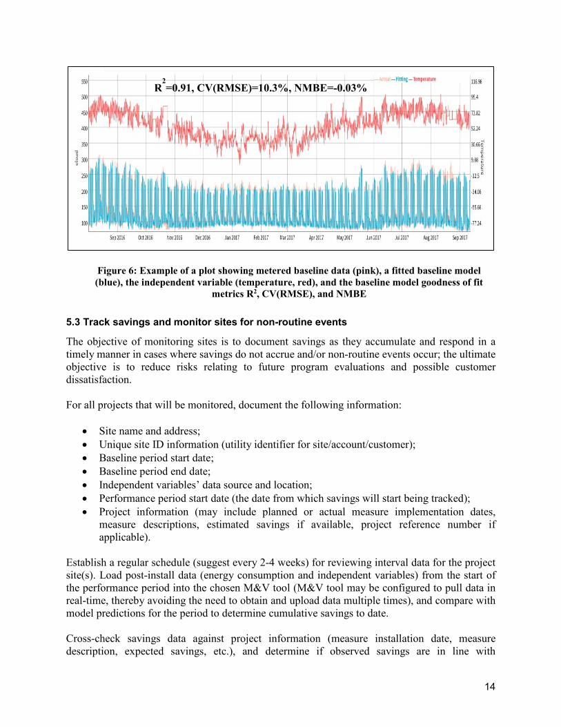
• Develop a baseline model and determine the model fitness metrics (see prerequisites). o Develop plots to visually assess model fit; a time series plot of actual and fitted

data, with independent variables, is recommended (see example in Figure 6). o Other charts that may be useful for visual review include scatter charts of

consumption vs. outside air temperature, or charts of residual values. • If model fitness metrics meet program requirements and charts indicate that data is

consistent and complete, baseline model may be accepted for the project. o If model fitness values do not meet program requirements and/or charts indicate

data-related issues, consider another model, additional/different independent variables, or a different M&V method.

14

Figure 6: Example of a plot showing metered baseline data (pink), a fitted baseline model (blue), the independent variable (temperature, red), and the baseline model goodness of fit

metrics R2, CV(RMSE), and NMBE

5.3 Track savings and monitor sites for non-routine events

The objective of monitoring sites is to document savings as they accumulate and respond in a timely manner in cases where savings do not accrue and/or non-routine events occur; the ultimate objective is to reduce risks relating to future program evaluations and possible customer dissatisfaction. For all projects that will be monitored, document the following information:

• Site name and address; • Unique site ID information (utility identifier for site/account/customer); • Baseline period start date; • Baseline period end date; • Independent variables’ data source and location; • Performance period start date (the date from which savings will start being tracked); • Project information (may include planned or actual measure implementation dates,

measure descriptions, estimated savings if available, project reference number if applicable).

Establish a regular schedule (suggest every 2-4 weeks) for reviewing interval data for the project site(s). Load post-install data (energy consumption and independent variables) from the start of the performance period into the chosen M&V tool (M&V tool may be configured to pull data in real-time, thereby avoiding the need to obtain and upload data multiple times), and compare with model predictions for the period to determine cumulative savings to date. Cross-check savings data against project information (measure installation date, measure description, expected savings, etc.), and determine if observed savings are in line with

R2=0.91, CV(RMSE)=10.3%, NMBE=-0.03%

15

expectations. If savings are unexpectedly low or high, or energy consumption anomalies are observed, consult with project team to determine what further investigation is warranted. Step changes in energy savings could indicate that an efficiency measure was installed or that a non-routine event occurred such as a change in building occupancy or operating hours. If non-routine events occur during the performance period, document the event and make the necessary calculations to account for the event. Documentation may include:

• Description to include timing (start and end date if temporary; start date if a permanent change), nature of the non-routine event, and any information collected to quantify the magnitude of the event. If non-routine event was identified using analytical means (e.g., based on anomaly in interval data use), include data and/or annotated charts as needed (See Appendix C for an example); and

• Calculations or models used to quantify the necessary adjustment to savings claim, including data and assumptions used in the analysis.

5.4 Document project savings claim

The objective when documenting a project savings claim is to transparently and accurately document savings in a way that is replicable for program evaluation purposes. For each meter-based savings calculation, M&V results should include:

• A list and description of measures implemented, along with key dates for baseline period, measure installation, and performance period;

• A narrative of the model that was used to quantify savings; • A description of the independent variables’ coverage factor; • An assessment of model fitness and time-series plot of the baseline period (see Figure 6); • A time-series plot of the post-measure performance period; • Additional plots to illustrate project impacts, as needed; • Meter-based gross savings; • TMY or other normalized savings (as required for program savings claims); and • A description of non-routine events and accounting of non-routine adjustments.

6. Regulatory engagement

The Pacific Northwest’s regional program delivery and regulatory community was engaged to determine requirements and acceptance criteria for the use of advanced M&V. This included consideration of key decision makers, reporting and documentation of results, and target levels of uncertainty and confidence in savings results. Key findings from multiple discussions with entities such as the Regional Technical Forum (RTF), Energy Trust of Oregon, Washington Utilities and Transportation Commission, Snohomish County Public Utility District, Puget Sound Energy, Seattle City Light, and BPA are summarized in the following.

16

Stakeholders that were engaged through this work were presented with a strawman of suggested elements to include in documentation and reporting of meter-based savings results. The strawman synthesized common elements from the Pacific Northwest as well as national guidance materials, and best practices in application of meter-based M&V. As appropriate and relevant, the concepts may be adapted for use in existing or future processes that stakeholders may be exploring. The strawman was modified based on feedback received, and converted to a living document5 (and associated slide deck6) that is available online. The RTF is the technical advisory committee to the Northwest Power and Conservation Council established in 1999 to develop standards to verify and evaluate energy efficiency savings. Historically, the RTF has focused on deemed savings approaches for specific technologies, as well as process level issues; these approaches are then adopted by commissions and utilities in the region. In the absence of existing RTF guidance, BPA has become the region’s recognized leader in thought and practice concerning requirements for rigor in meter-based whole-building savings estimation. Programs delivered through BPA’s Option 2 utilities represent high potential for adoption of meter-based savings estimation. While not explicitly stated in stakeholder discussions, parties external to RTF did not appear to be aggressively lobbying for RTF to take strong near-term action (such as creating guidance documents or program policies), perhaps suggesting that at the current scale, there is no immediate need for additional direction (An additional limitation is faced by regions and utilities that have limited penetration of smart meters). However, there was a desire for RTF to define the current state of technical guidance for advanced M&V, what gaps exist in the guidance and, where appropriate, to take a position on the application of advanced M&V in the Pacific Northwest. In May 2019, RTF published a position paper [Koran 2019] that included recommendations (with backup reference material) on the following topics:

• Model type selection: Existing tools and guidance are highly capable. ECAM and the Time-of-Week-and-Temperature model were covered in some detail. Some reservations were expressed regarding the CalTRACK model specification.

• Model/savings uncertainty: Quantifying savings uncertainty is the key metric (baseline model fitness metrics considered secondary). Inability to calculate uncertainty for hourly models is a significant constraint.

• Non-routine events: NREs can strongly impact savings estimates in some cases, but the size of that threat is unknown. Research is needed to better quantify/characterize NREs and to improve practitioner guidance and tools.

• Model automation and aggregation of results: Some existing industry guidance (notably CalTRACK) is strongly oriented toward aggregation-driven approaches and has roots in residential applications. As such, RTF recommends more research to establish reliability of aggregated approaches, for example assessing the impacts of NREs at aggregate level and quantifying uncertainty.

5 https://buildings.lbl.gov/sites/default/files/LBNL%20Guidance%20on%20M%26V%202.0%20savings%20claims%202019-06-30.pdf 6 https://buildings.lbl.gov/sites/default/files/AcceptanceCriteriaAndDocumentation%202019%2006%2030.pdf

17

7. Seattle City Light demonstration

The Seattle City Light commercial M&V 2.0 pilot demonstration was initiated in 2017, commencing with pilot site selection. Seattle City Light reviewed project lists to identify ongoing or proposed projects that saved 5% of whole building energy consumption or more. M&V 2.0 has shown potential when looking to quantify savings for complex projects, e.g., addition of controls, multiple measures, retro-commissioning. Upon review Seattle City Light was unable to identify suitable ongoing or proposed projects, but developed a list of past projects where claimed savings exceeded 5% of whole building electric consumption. In many cases the project locations saw multiple projects installed, of varying savings magnitude, sometimes over several years. Seattle City Light provided historical hourly electric consumption for all project sites (going back to 2013), and continued providing new batches of hourly data each month as the demonstration progressed. Seattle City Light and Berkeley Lab reviewed project dates, project information, and time-series plots of kWh consumption data, in order to determine whether advanced M&V savings analysis was feasible. Based on this review process, 18 projects were identified for the demonstration, with measures implemented at the latest in early 2018. The project sites screened out at this stage were a result of unreliable measures implementation dates and/or data quality issues. The TOWT model was used to characterize each building’s baseline electricity consumption (kWh) for the demonstration. In order to determine baseline acceptability Berkeley Lab quantified three model fitness metrics for each proposed demonstration site:

• R2, target >0.7; • CV(RMSE), target <25%; • NMBE, target within -0.5% to +0.5% range.

Advanced M&V savings were estimated for a 12-month period (the “reporting period”) following measure implementation. Using hourly weather data for the reporting period, each site’s energy model was used to generate hourly consumption predictions, and these were compared with actual consumption to determine advanced M&V savings estimates. Figure 7 shows an example time series chart for a site’s baseline period, Figure 8 shows an example reporting period time series chart for the same site, and Figure 9 shows the CUSUM chart for the same site.

18

Figure 7: Example of a plot showing metered baseline data (pink), a fitted baseline model (blue), the independent variable (temperature, red), and the baseline model goodness of fit

metrics R2, CV(RMSE), and NMBE

Figure 8: Example of a plot showing metered reporting period data (pink), model-predicted consumption (green), and the independent variable (temperature, red)

Figure 9: Example CUSUM chart, illustrating clean, consistent savings accumulation through the reporting period (total 902,369kWh estimated savings)

R2=0.94, CV(RMSE)=5%, NMBE=-0.02%

19

Three types of savings profiles were observed for the pilot sites:

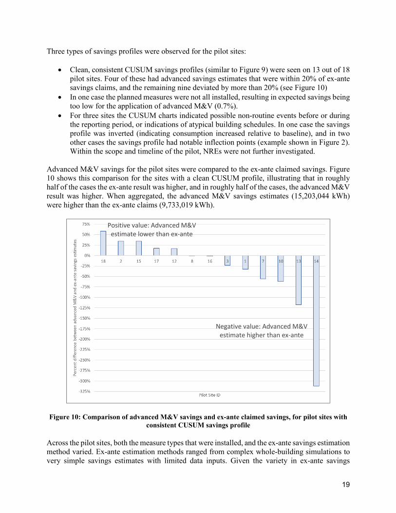
• Clean, consistent CUSUM savings profiles (similar to Figure 9) were seen on 13 out of 18 pilot sites. Four of these had advanced savings estimates that were within 20% of ex-ante savings claims, and the remaining nine deviated by more than 20% (see Figure 10)

• In one case the planned measures were not all installed, resulting in expected savings being too low for the application of advanced M&V (0.7%).

• For three sites the CUSUM charts indicated possible non-routine events before or during the reporting period, or indications of atypical building schedules. In one case the savings profile was inverted (indicating consumption increased relative to baseline), and in two other cases the savings profile had notable inflection points (example shown in Figure 2). Within the scope and timeline of the pilot, NREs were not further investigated.

Advanced M&V savings for the pilot sites were compared to the ex-ante claimed savings. Figure 10 shows this comparison for the sites with a clean CUSUM profile, illustrating that in roughly half of the cases the ex-ante result was higher, and in roughly half of the cases, the advanced M&V result was higher. When aggregated, the advanced M&V savings estimates (15,203,044 kWh) were higher than the ex-ante claims (9,733,019 kWh).

Figure 10: Comparison of advanced M&V savings and ex-ante claimed savings, for pilot sites with consistent CUSUM savings profile

Across the pilot sites, both the measure types that were installed, and the ex-ante savings estimation method varied. Ex-ante estimation methods ranged from complex whole-building simulations to very simple savings estimates with limited data inputs. Given the variety in ex-ante savings

Negative value: Advanced M&V estimate higher than ex-ante

Positive value: Advanced M&V estimate lower than ex-ante

20

estimation methods it is not surprising to see differences in values when comparing to advanced M&V estimates. At the time of pilot completion Seattle City Light was continuing its review of savings estimates and the CUSUM profiles, to determine whether any follow up actions were warranted on individual projects (e.g., for high-savings projects with significant difference between ex-ante and advanced M&V estimates, would it be helpful to reach out to the customer to inquire about the measures and any other activities at the building that might have affected energy consumption?). The average time to conduct advanced M&V for the pilot was five hours per project. The majority (66%) of this time was for data processing/preparation, followed by collating and reviewing results (33%), and a minimal amount of time on the energy modeling itself (1%). Records of effort/time to create utility ex-ante savings estimates were not available for the pilot sites’ projects; however, the calculation methods applied for each project were documented, and typical time estimates were estimated for each of these four methods (See Table 1). The wide range in effort for some of these methods reflects the varying levels of complexity in measure types. At an average of five hours per project, advanced M&V required less effort than all but the very simplest of the traditional methods used to create ex-ante savings estimates. Table 1: Time estimates for program ex-ante savings calculations

Ex-Ante Savings Estimate Methodology Estimated

Effort (Hr./ Project)

Simple estimate (e.g., deemed, using past experience as a general guide) Inputs: Quantities (pre- and post-inspections), equipment power rating (nameplate), run hours (client schedule or assumed). Informed by previous projects.

3 - 35

Engineering calculations (e.g., bin model, using short term logged data). Inputs: Logged data and published information, and possibly TMY3 temperature data.

17 - 66

Hourly spreadsheet analysis (i.e., 8760-hour spreadsheet calculation). Inputs: TMY3 OAT data, logged data (kW, kWh, air temperatures, run hours, air flows, and/or VSD speeds), and published information.

18 - 71

Simulation model. Inputs: Schedules, kW (lighting, plug, people, internal loads), equipment kW (logged), and/or cooling load (logged), OAT, and published information. Informed by comparison with actual consumption.

15 - 76

In reviewing the level of effort to conduct advanced M&V, compared to the time estimates for other methods in Table 1, it is seen that advanced M&V can be a practical savings estimation option for utilities. Advanced M&V could be used in combination with traditional ex-ante methods as a way to increase confidence in results, in some cases may be ideal as the primary verification method for complex projects, could provide an early indication of true savings impact at the meter, and could be used within a pay-for-performance program.

21

8. Conclusions Key lessons learned relative to the project objectives, and applicability of project findings for BPA, are summarized below. Objective: Develop practitioner workflows that integrate advanced M&V tools with supplementary automated routines for non-routine adjustments and for quantification of savings uncertainty to indicate rigor.

What we learned: Simple workflows were developed, and in combination with accuracy/documentation guidelines these are straightforward to apply. Guidance and case study examples of NRAs remain a gap (reinforced by RTF’s paper). We also learned that existing uncertainty calculations are unreliable for hourly models, hence recommend model fit criteria and out-of-sample testing for tool validation BPA applicability:

The workflows are ready to use, and complemented by accuracy/documentation guidance and EVO tool testing7.

NRE identification code is ready to use, though recommended only as ‘filtering’ tool which is then reviewed by experienced practitioners (in conjunction with CUSUM charts)

A meaningful start toward methods for non-routine adjustments was developed, but additional R&D is needed to further mature and test them. This could be complemented by RTF’s call for a catalogue of example buildings’ data with NREs documented.

Objective: Demonstrate practitioner workflows with Seattle City Light, in collaboration with their implementers and evaluators – determine labor and time/cost savings, and uncertainty of the results obtained.

What we learned: The advanced M&V tools and methods are effective, and the utility partner was enthusiastic about having a dynamic, data-driven view of project performance. The process is relatively streamlined (once data access/formatting is configured), so application on ‘real-time’ projects should be very cost-effective. Future applications will benefit from continued attention to assess the number of projects can realistically meet the 5% savings criteria, and to documenting utilities’ process for addressing underperforming projects, NREs, and negative savings. BPA applicability:

M&V 2.0 offers complementary benefits to existing savings estimation methods. Advanced M&V could be used in combination with traditional ex-ante methods as

a way to increase confidence in results, in some cases may be ideal as the primary verification method for complex projects, could provide an early indication of true

7 Advanced M&V software testing portal, based on a test method developed by Berkeley Lab, has been made publicly available by EVO at: http://mvportal.evo-world.org/

22

savings impact at the meter, and could be used within a pay-for-performance program.

BPA can view these methods as ‘program-ready,’ though needing technical input during ramp-up phase, and noting earlier comments on NREs.

Objective: Engage the Pacific Northwest regulatory community to determine acceptance criteria for the required accuracy and reporting of advanced whole-building M&V.

What we learned: There is interest in the topic of advanced M&V, and stakeholders have looked to BPA and RTF to provide technical and programmatic guidance. Best practice methods are well defined, and there are two notable areas where challenges exist. Firstly, savings uncertainty calculation methods exist (referenced in advanced M&V guidance), but now that uncertainty calculations have been shown to be unreliable for daily or hourly models, there is a need to seek technical solutions that will allow for reliable uncertainty quantification for applications that extend beyond monthly data and monthly models. Secondly, conceptual guidance exists for identifying and adjusting for NREs, and this project has produced early research on data-driven methods. Clear program guidance based on current knowledge will enable the industry to continue deployment while also providing opportunity to learn more about the frequency and severity of NREs in the field. BPA Applicability:

The outcomes of this project, in combination with the parallel efforts through Seattle City Light’s pay-for-performance program, provide BPA with practical resources that can inform updates to technical guidance, and helps BPA-affiliated utilities to adopt advanced M&V methods while managing the risks associated with under-performing projects.

The final objective was to document the findings to facilitate broad industry uptake of the solutions. The outcomes of this project can help utilities develop rigorous, practical program designs, understanding the process implications and managing the risks involved. Given the lack of publicly documented examples of the application of advanced M&V, this project constitutes a major step forward in supporting uptake of these new methods in the Pacific Northwest.

9. Next steps and future opportunities This project demonstrated the practical application of advanced M&V tools and methods, and surfaced additional opportunities to support scaled adoption. These include:

• Continued work to characterize, and develop and test analytics-based solutions to identify

and adjust for non-routine events. • Exploration of auto-regressive models to potentially overcome challenges in quantifying

uncertainty due to model error, for hourly or daily data granularity. • Further engagement of the regulatory community on key issues such as model type

selection, NREs, uncertainty quantification, and further validation of approaches to address situations where independent variables in the reporting period fall outside the range observed in the baseline.

23

Another general area of research that could prove beneficial is to explore the connection between advanced M&V at the building/program level and grid-level concerns. Given the time-varying value of energy and demand reductions, and the changing mix of generation options at grid level, better understanding of building load shapes and savings load shapes will become more critical to utilities and grid planners. Advanced M&V methods could be a useful tool in that context, though that potential has not yet been extensively explored.

Acknowledgements This work was supported by the Assistant Secretary for Energy Efficiency and Renewable Energy, Building Technologies Office, of the U.S. Department of Energy under Contract No. DEAC02-05CH11231. The authors would like to thank the Bonneville Power Administration (BPA) Technology Innovation Program and Seattle City Light for supporting this study, with special thanks to Erik Boyer (formerly BPA), Todd Amundson (BPA), Sarah Zaleski (U.S. DOE Building Technologies Office), John LeCompte and Colm Otten (Seattle City Light).

24

References Chouakria, A. D., & Nagabhushan, P. N. (2007). Adaptive dissimilarity index for measuring time series proximity. Advances in Data Analysis and Classification, 1(1), 5-21. Crowe, E, Granderson, J, Fernandes, S. From Theory to Practice: Lessons Learned from an Advanced M&V Commercial Pilot. Proceedings of the 2019 International Efficiency Program Evaluation Conference. Franconi, E, Gee, M, Goldberg, M, Granderson, J, Guiterman, T, Li, M, Smith BA. 2017. The status and promise of advanced M&V: An overview of “M&V 2.0” methods, tools, and applications. Rocky Mountain Institute and Lawrence Berkeley National Laboratory. Berkeley Lab report Berkeley Lab-1007125. Granderson, J, Fernandes S. 2017. State of advanced measurement and verification technology and industry application. The Electricity Journal 30:8-16. DOI: 10.1016/j.tej.2017.08.005. Killick, R, and Eckley, I. 2014. Changepoint: An R package for changepoint analysis. Journal of Statistical Software 58(3), pp.1-19. Koran, B, Rushton, J. 2019. Reliability of Energy Savings Estimates Based on Commercial Whole Building Data. Prepared for the Regional Technical Forum. Kramer, H, Russell, J, Crowe, E, Effinger, J. 2013. Inventory of commercial energy management and information systems (EMIS) for M&V applications. Northwest Energy Efficiency Alliance. Report #E13-264. Touzani, S, Granderson, J, Jump, D, Rebello, D. 2019. Evaluation of methods to assess the uncertainty in estimated energy savings. Energy and Buildings 193:216-225. DOI: https://doi.org/10.1016/j.enbuild.2019.03.041. Touzani, S, Ravache, B, Crowe, E, Granderson, J. 2019. Statistical change detection for building energy consumption: applications to savings estimation. Energy and Buildings 185:123-136. DOI: https://doi.org/10.1016/j.enbuild.2018.12.020