HAL Id: hal-00955420https://hal-enac.archives-ouvertes.fr/hal-00955420

Submitted on 4 Mar 2014

HAL is a multi-disciplinary open accessarchive for the deposit and dissemination of sci-entific research documents, whether they are pub-lished or not. The documents may come fromteaching and research institutions in France orabroad, or from public or private research centers.

L’archive ouverte pluridisciplinaire HAL, estdestinée au dépôt et à la diffusion de documentsscientifiques de niveau recherche, publiés ou non,émanant des établissements d’enseignement et derecherche français ou étrangers, des laboratoirespublics ou privés.

Realistic Network Traffic Profile Generation : Theoryand Practice

Antoine Varet, Nicolas Larrieu

To cite this version:Antoine Varet, Nicolas Larrieu. Realistic Network Traffic Profile Generation : Theory and Practice.Computer and Information Science, Canadian Center of Science and Education, 2014, 7 (2), pp 1-16.�10.5539/cis.v7n2p1�. �hal-00955420�

Realistic network traffic profile generation: theory and practice

Antoine Varet1 & Nicolas Larrieu1

1 ENAC Telecom/Resco Laboratory, Toulouse, France

Correspondence: Nicolas Larrieu, ENAC, E-mail: nicolas.larrieu@enac.fr

Abstract

Network engineers and designers need additional tools to generate network traffic in order to test and evaluate

application performances or network provisioning for instance. In such a context, traffic characteristics are the

very important part of the work. Indeed, it is quite easy to generate traffic but it is more difficult to produce

traffic which can exhibit real characteristics such as the ones you can observe in the Internet. With the lack of

adequate tools to generate data flows with “realistic behaviors” at the network or transport level, we needed to

develop our tool entitled “SourcesOnOff”. The emphasis of this article is on presenting this tool, how we

implemented it and which methodology it follows to produce traffic with realistic characteristics. To do so, we

chose to consider different stochastic processes in order to model the complexity of the different original traffics

we wanted to replay. In our approach, we are able to consider several statistical laws and to combine their effects

to model accurately the original behavior we analyzed in the real data. We then select the right parameters to

consider as inputs for our SourcesOnOff tool. This approach gives really good traffic characteristics and,

consequently, the generated traffic is really closed to reality as results presented at this end of this paper

demonstrate it.

Keywords: Traffic generation, Network experimentation, Network performance analysis, Network measurement

1. Introduction

Network engineers and designers need additional tools to generate network traffic in order to test and evaluate

application performances or network provisioning for instance. In such a context, traffic characteristics are the

very important part of the work. Indeed, it is quite easy to generate traffic but it is more difficult to produce

traffic which can exhibit real characteristics such as the ones you can observe in the Internet.

With the lack of adequate tools to generate data flows with “realistic behaviors” at the network or transport level,

we needed to develop our tool entitled “SourcesOnOff ”. In this paper, “realistic behavior” means to generate

traffic similar to the traffic a network administrator can capture on his network backbone, end-systems, etc...

Previous research conducts us to design new methodologies and tools to generate network data traffic as close as

possible to what we can find on Local Area Networks (LAN) and on the Internet. It can be necessary for instance

to evaluate performances of new network entities (such as an embedded router (Varet et al., 2012)). In this

specific context, we needed to face this router to generated traffic with characteristics as close as possible as the

Internet traffic. However, depending on what you mean by “Internet network” and where you perform the study,

measurements may completely differ: Internet cannot be solely characterized with a small set of parameters such

as some mathematical distributions and additional factors. Indeed, there is not currently one unique mathematical

modeling able to embrace the different characteristics and the complexity of the Internet traffic (Olivier &

Benameur, 2000). Anyway, Internet traffics hopefully show some common properties and trends (detailed in the

next paragraph) that helps to its modeling.

For instance, an Internet Service Provider (ISP) providing access for software engineering companies manage a

different profile of data communications than an ISP for private individuals (Gebert et al., 2011). However, there

are some common characteristics between both profiles. The goal of the tool we have developed is to handle

most of Internet traffic profiles and to generate traffic flows by following these different Internet traffic

properties.

The rest of this paper is structured as the following. The first section presents the mathematical model this tool is

based on for traffic generation: the ON/OFF sources. We chose to consider different stochastic processes in order

to model the complexity of the original traffic we want to replay. General approaches consider only one law for

the On process and another law for the Off process. In our approach, we are able to consider several laws and to

combine their effects to model accurately the original behavior we analyzed in the real data. We then select the

right parameters to consider as inputs for our SourcesOnOff tool. This approach gives really good traffic

characteristics and, consequently, the generated traffic is really closed to reality as results presented at this end of

this paper demonstrate it. In the second section, we present why the other tools currently available were not

usable in our case. The third section describes how our tool works plus some specific points the user should

know about its implementation. The fourth section is dedicated to the validation of our tool with different

methods in order to conclude if the generated traffic has the same properties than the original one. We have, in

particular, investigated the traffic characteristics generated by our software and we demonstrate that it is able to

generate network traffic with realistic properties such as these we can capture on the Internet. Different

parameters have been considered to match generated traffic characteristics with the original traffic. First, we

considered classical traffic parameters such as throughput, delay or losses but we have also investigated more

advanced statistical parameters such as the correlation level of generated packets or their long range dependence

(by computing the Hurst factor).

1.1 How to characterize an “Internet-like” profile?

Different studies were published with results related to Internet-like traffic characterization: the word “Internet”

can cover very different profiles, but some common trends can be highlighted. Thus, we will examine two of

them: high variability and self-similarity, respectively called the Noah and Joseph Effects.

High variability is characterized by an infinite mathematical variance and means that sudden discontinuous

changes can always occur. Some mathematical distributions like Pareto and Weibull are heavy-tailed (i.e. the tail

of the distribution is not exponentially bounded) and thus can be used to generate sets of values with high

variances and also high-variability.

Different studies have shown that classical distributions such as the Gaussian and the Poisson distribution have

failed to reproduce a LAN-like throughput (Leland et al., 1994) (Olivier & Benameur, 2000). One of them

(Olivier & Benameur, 2000) proposes to use Pareto’s and Weibull’s heavy-tailed distributions and proved that the

generated traffic shows properties closer to real network traffic characteristics than other mathematical

distributions.

Self-similarity is defined by a long-range dependence characteristic, which means there are bursts of traffic any

time over a wide range of time scales. In other words, a small sub-range of values is “similar” to the whole range

of values. W. Willinger found in (Willinger et al., 1997) a relation between self-similarity and high variability for

Ethernet Local Area Network (LAN) throughputs: in particular, he showed that the Noah and the Joseph effects

are linked with a degree-1 polynomial relation. In other words, using ON/OFF sources with heavy-tailed

distributions causes the traffic streams to be highly variable and, consequently, the aggregation of these streams

to be also self-similar and highly variable.

1.2 ON/OFF sources to generate realistic throughputs

W. Willinger proposed in (Willinger et al., 1997) to generate data following packet-train models, i.e. with strictly

alternating, independent and identically distributed ON- and OFF-periods and proved that these ON/OFF

sources generate data similar to experimental measurements on real networks.

A source corresponds to one network flow. The flow is associated with a source and destination couple and also

with data, transmitted as a set of packets called a train of packets. In our case, we use the transport protocols TCP

and UDP. The data stream is thus exchanged as a set of IP packets. The source is associated to a departure time

and a duration time.

The departure time of any source is computed with the departure time of the preceding source plus a random

duration. This randomness follows the user-defined “Doff distribution” (also named “distribution of inter-train

durations”). The first source starts at the beginning of the process.

Duration times should be similar for all sources. They should follow a user-defined random distribution called

“Don distribution” (also named “distribution of train duration” or “distribution of flow duration”). This Don

distribution is independent of the Doff distribution.

For feasibility constraints and to reduce the complexity of implementation, we use the Don distribution to

generate random values, not for time duration in seconds but for quantity of transmission in bytes. Because of

TCP congestion control mechanisms, source durations are correlated with quantities of transmitted data.

We can summarize the ON-OFF source generation algorithm we use in our tool by:

For n from 1 to infinite do:

1. /* start a new source here */

2. Don_value := get a random value of distribution Don;

3. Doff_value := get a random value of distribution Doff;

4. Wait for the duration Doff_value

5. Start the transmission of Don_value bytes to a remote host (do not wait the end to perform the next iteration,

loop as soon as data are sent into the transmission buffer)

End_For

Algorithm 1: Traffic generation with ON/OFF sources

In algorithm 1, the Don_value is the length (in bytes or multiples of bytes) of each data flow, also called a “train”.

This train is exchanged between the local (transmitter) system and a remote (receiver) system. The Doff_value

(in seconds or more often in milliseconds) is a duration called the inter-train distance (i.t.d). This i.t.d. represents

the time between two consecutive flow creations. The Doff_values and the Don_values are completely

independent. They are issued from random number generators, which follow respectively the “Don” and the

“Doff” distributions. These distributions should be heavy-tailed to ensure the self-similarity of the generated data

throughput (Willinger et al., 1997). Distribution parameters are defined by the user on the command-line.

For example, if we have the following sequence of sources <A, B, C, …> and if Doff values, randomly

generated, begin with the sequence <A.Doff=3, B.Doff=3, C.Doff=5, …> and Don values with <A.Don=10,

B.Don=3, C.Don=4, …>, then figure 1 illustrates which throughput we can expect on the network.

Internet flows are mainly TCP and UDP flows. From an application point-of-view, the TCP protocol uses

congestion avoidance mechanisms and then spreads the data transmission out in time: the stream is divided into

segments and each segment is sent when the previous segment has been correctly received. Flow durations

depend of many unpredictable factors in real systems where other flows share the same resources. Moreover, the

UDP protocol divides the data into multiple datagrams and sends all datagrams as fast as the lower layers can,

with possible losses. The proportion of TCP vs. UDP is a parameter of the Internet profile.

Figure 1: Emission process of ON/OFF traffic sources

2. State of the art of traffic generators

2.1 Network simulators

Different tools are available to simulate networks and their behaviors, with integrated ON/OFF sources. We can

cite, for instance, NS-2 (NS-2, 2013), OpNet (OpNet, 2013) or OmNet++ (OmNet++, 2013).

Most of them provide “Internet-like” flow generators, some of them based on ON/OFF source generation

processes. However, the aim of our research work was to face new network systems to real traffic. It means we

wanted to perform our system evaluation in real time and do not want to evaluate a model of our system.

Simulators cannot do this kind of real time experiments, only emulators can do it. However, it is complex to deal

with most network emulators as they are complex to install, to configure with the real network environment, and

consume as well many CPU resources. This is why we searched for and studied tools not to simulate or emulate

but to generate a realistic traffic load on real networks.

2.2 Traffic replay tools

Some software enables the user to replay previously captured network traffics. This is done in two steps. Firstly,

the user captures data on the networks he wants to reproduce. This can be done with tools called “sniffers” such

as the reference tool Wireshark (Wireshark, 2013) and its background application “dumpcap” (Dumpcap, 2013),

a command-line tool called up internally by Wireshark. Secondly, he needs to replay the captured traces, i.e. by

retransmitting the sniffed packets in the same order, and separated with the same delays as these measured

during the capture (cf. the “tcpreplay” (note 1) tool for instance). Harpoon (note 2) is another existing Open

Source flow-level traffic generator, but this tool requires the user to define flow per flow the data weight he

wants to transmit on the network. The automatic generation of the network profile is limited to constant and

uniform distributions. Moreover, Harpoon seems to be not maintained since 2005. This is why we did not

consider this tool for our experiments.

This traffic replay process has different advantages. The two steps may be done independently by two different

users and at any time (as long as the first step is started before the second one). The capture may be filtered

before being replayed. Replay parameters may be set up: for example traffic replay may be faster or slower than

the capture speed, it may be altered with random losses or random transformations…

However, replaying has also important drawbacks. Indeed, before replaying any network trace, the user must

make or acquire the capture he wants to replay. Most of the time, this is a difficult task: user privacy issues

restrain the administrators in allowing captures on the router they administer; often ISPs do not want to extract

advanced statistics from their networks… The public data we have found on Internet are often so anonymized

that they not longer contain the useful information we need to replay them. Moreover, if you continuously replay

the same trace you will reproduce periodically the same “events” (throughput bursts, specific packet sequences

or behaviors…). This periodicity might falsify some statistical analysis and deceive network systems. For

instance, this type of traffic replay cannot be efficient if you want to assess performances of network

mechanisms such as transport protocols given its objective is to act on traffic profile and by definition this traffic

replay do not give any freedom to transport protocols to optimize traffic exchanges (such as congestion control

mechanisms for instance).

2.3 Network throughput estimation tools

This is why different techniques and tools have been elaborated to load a network and evaluate its capacity. One

of the existing tools we have studied is “iperf” (Iperf, 2013). It can generate TCP or UDP flows to load the

network. In TCP mode, an iperf client transmits to the server an infinite quantity of data through one TCP flow.

After a user-defined duration, the iperf tool aborts the TCP connection and prints on the screen different statistics

and the total quantity of data it succeeded in transmitting correctly.

A network capture shows often that mostly all the network resources are used by the TCP flows (Gebert et al.,

2011). On one hand, the TCP protocol efficiently exploits the network and transmits data in an optimal time span.

However, in LAN captures, external and unexpected events interact with the flow, they generate segment delays

and losses impacting the TCP connection which becomes longer than the optimal time span expected. This

drawback affects most of methodologies based on studies using only one TCP flow. We can cite, for example,

when the tester uses an SSH or an FTP connection to transmit a big file and consequently to artificially load the

network.

Figure 2c illustrates such a measure of throughput with iperf generating a TCP flow. We can see, from a first

qualitative point of view, that the throughput generated by iperf is nearly constant and predictable, contrary to the

throughput of an Internet capture (in figure 2a) and the throughput generated by our tool Sourceonoff (in figure

2b).

Iperf may be configured to transfer multiple TCP streams; in this case the program starts the different flows

simultaneously at the beginning of the program. This behavior is not realistic: resources are shared fairly from

the beginning, whereas in Internet later flows are penalized at their start by the flows already established.

Moreover, this tool “iperf” performs measurements on “long” TCP connections (about 10 second duration by

default); this allows the TCP congestion control mechanism to adjust the data throughput efficiently. However, in

most of ISP studies the TCP connections are very numerous and the majority is short (for instance, 81% of TCP

connections carry less than 310 bytes, in study (Iperf, 2013)). Consequently, congestion control mechanisms do

not have the time to optimize the connection.

In UDP mode, the client transmits data periodically: the period is computed depending on the user-defined

quantity of data per second to transmit. However, for the same reason than previously, a single flow with

constant throughput is not realistic (Gebert et al., 2011) (Olivier & Benameur, 2000).

Consequently, we have searched for other tools to generate data throughput: BWPing (BWPing, 2013), Ttcp

(Ttcp, 2010), NetPerf (NetPerf, 2013), NetPerfMeter (Dreibholz, 2011), Ostinato (note 3)… All differ more or

less on the set of supported protocols, on the maximum admissible throughputs and on the statistics printed on

the screen for the user. However, all have the same drawbacks as explained above.

This is why, in the rest of this article, we chose the tool “iperf” as a comparison reference for our SourcesOnOff

tool, because most measurement tools are based on the same assumptions and work in a similar manner: one or

multiple identical and simultaneous TCP and UDP flows in order to load the network at its maximum available

capacity.

Figure 2: Throughputs generated by iperf and our tool

3. The SourcesOnOff tool

We did not find in the state of the art we performed any tool to generate data flows based on exact ON/OFF

sources. This is why we developed this one in C language and validated it with the Debian Operating System.

The tool we propose is free and Open Source, under the General Public License v3 (GPLv3 (GPL, 2013)).

Source code can be downloaded at http://www.recherche.enac.fr/~avaret/sourcesonoff.

Initially developed for Debian-based systems, the 10 source files with 3,000 lines of code are compiled with the

GNU C Compiler (gcc, with GCC (GCC, 2013)) and with the pedantic option. It is not POSIX-compatible

because we use intensively the (long long) 64 bit-integer type and the (long double) float type for mathematical

computations. Moreover, the tool uses certain Linux-specific functions (e.g. the epoll() system call) and so it

should not be easily portable on non-Linux based systems, such as Microsoft Windows® or Mac OSX®. This

software is linked with the real-time (-lrt) and the mathematical (-lm) libraries. The binary is between 84kB (32

bit version) and 111kB (64 bit version).

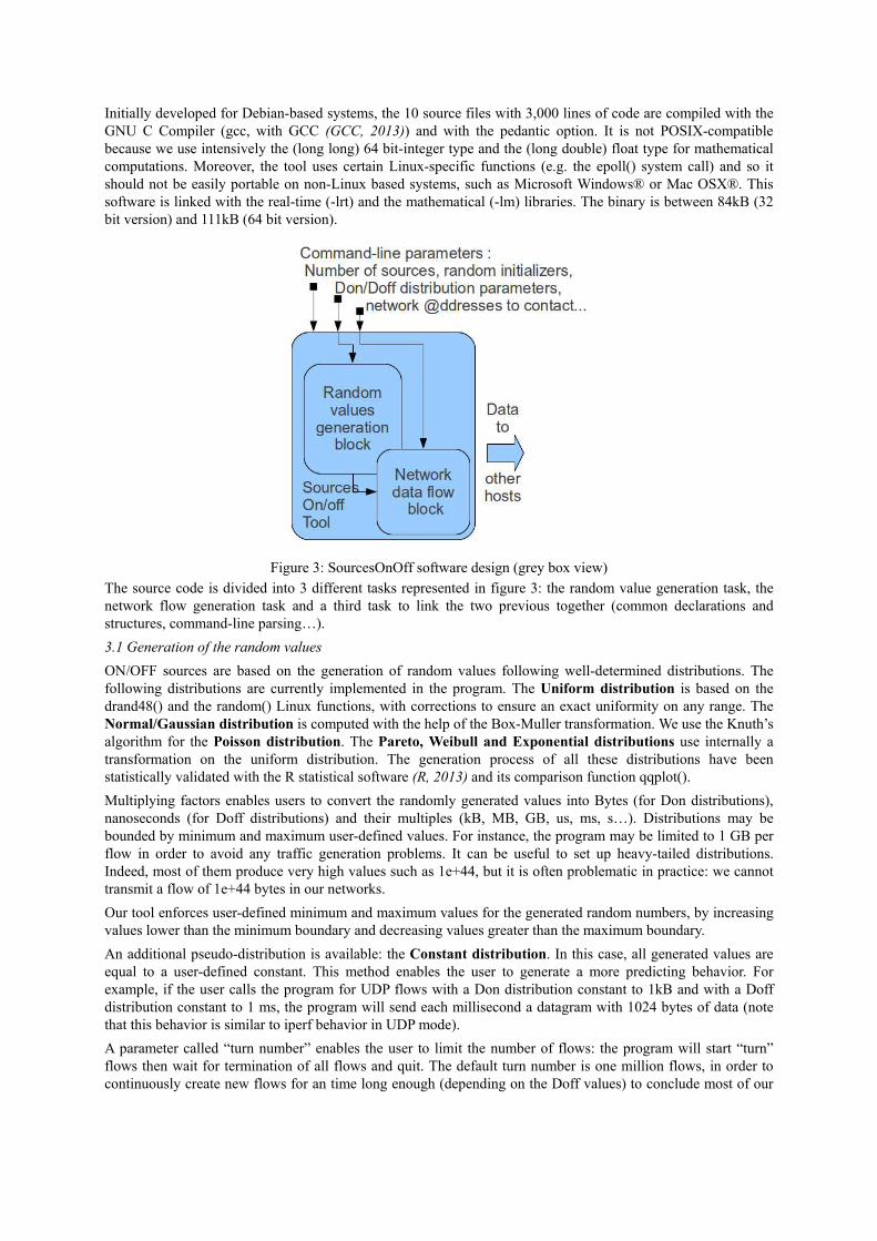
Figure 3: SourcesOnOff software design (grey box view)

The source code is divided into 3 different tasks represented in figure 3: the random value generation task, the

network flow generation task and a third task to link the two previous together (common declarations and

structures, command-line parsing…).

3.1 Generation of the random values

ON/OFF sources are based on the generation of random values following well-determined distributions. The

following distributions are currently implemented in the program. The Uniform distribution is based on the

drand48() and the random() Linux functions, with corrections to ensure an exact uniformity on any range. The

Normal/Gaussian distribution is computed with the help of the Box-Muller transformation. We use the Knuth’s

algorithm for the Poisson distribution. The Pareto, Weibull and Exponential distributions use internally a

transformation on the uniform distribution. The generation process of all these distributions have been

statistically validated with the R statistical software (R, 2013) and its comparison function qqplot().

Multiplying factors enables users to convert the randomly generated values into Bytes (for Don distributions),

nanoseconds (for Doff distributions) and their multiples (kB, MB, GB, us, ms, s…). Distributions may be

bounded by minimum and maximum user-defined values. For instance, the program may be limited to 1 GB per

flow in order to avoid any traffic generation problems. It can be useful to set up heavy-tailed distributions.

Indeed, most of them produce very high values such as 1e+44, but it is often problematic in practice: we cannot

transmit a flow of 1e+44 bytes in our networks.

Our tool enforces user-defined minimum and maximum values for the generated random numbers, by increasing

values lower than the minimum boundary and decreasing values greater than the maximum boundary.

An additional pseudo-distribution is available: the Constant distribution. In this case, all generated values are

equal to a user-defined constant. This method enables the user to generate a more predicting behavior. For

example, if the user calls the program for UDP flows with a Don distribution constant to 1kB and with a Doff

distribution constant to 1 ms, the program will send each millisecond a datagram with 1024 bytes of data (note

that this behavior is similar to iperf behavior in UDP mode).

A parameter called “turn number” enables the user to limit the number of flows: the program will start “turn”

flows then wait for termination of all flows and quit. The default turn number is one million flows, in order to

continuously create new flows for an time long enough (depending on the Doff values) to conclude most of our

experiments. The special values of 1 flow for the turn parameter and a Don distribution constant to 1 GB is

similar to transferring 1 gigabyte of random data through one TCP connection. In most cases, this overloads the

network capacity of the path until all the data are transmitted.

3.2 Generation of the network flows

First of all, different sets of Don and Doff random values are generated. They are then used for data

communications. Command-line parameters specify, for each set of (Don; Doff) values, the different socket

properties: are they transmitters and so who is the destination host? Or is it a bottomless pit? Do we use UDP or

TCP protocol? What is the port number to use? Does IPv4 or IPv6 be used with? Does a set of sources be

delayed before starting (to let another set of sources take some advance)? Does the set of sources be stopped

after a delay, even if there are still active sources? How many maximum sources should be created? Does the

random generator be initialized with a specific seed (i.e. to reproduce two exact source generations)?

All these parameters enable the user to refine the tool behavior. Different sets of sources may run simultaneously,

each set is associated with independent Don and Doff distributions and parameters. For instance, a set of sources

may be defined to load the network with TCP streams and another set to generate UDP datagrams. The process

forks itself to provide TCP and UDP data simultaneously. Each task uses the epoll() primitive to perform the

management of thousand of flows if necessary. This primitive reduces the portability of the software to only

Linux systems and should be replaced with the POSIX-compatible select() primitive in a future tool release.

Contrary to programs like iperf, this tool is only intended to generate data. It was not developed to provide itself

advanced statistics on the network: we use our tool to generate background traffic and additional passive and

active measurement tools to evaluate network performances and collect statistics (note 4).

3.3 Statistic profile extraction from a real traffic trace

Before experimenting traffic generation, we have to define what kind of traffic we want to generate. This step

may be done arbitrarily by choosing appropriate values or by selecting values from existing studies like (Gebert

et al., 2011) (Olivier & Benameur, 2000).

We chose an alternative solution: given that we belong to a research entity, we have easily access to real data.

Thus, we asked to our local network administrator to capture the entire incoming and outgoing traffic, generated

by people from the university (students, administrative people, teachers and researchers) on our local area

network. The data were captured on the firewall protecting the access link between our LAN and other networks:

REMIP (REMIP, 2013) and RENATER (RENATER, 2013). REMIP and RENATER networks are our links to the

Internet. Thus, we captured all data from our LAN to Internet and all associated responses.

We captured a set of 9 millions of IPv4 packets, mostly TCP data (97.7% of TCP, 2.2% of UDP and 0.1% of

ICMP), during 10 hours between 8:00AM and 6:00PM, Tuesday the 29th of January, 2013. We expected to

generate simultaneously TCP sources and UDP sources with our tool SourcesOnOff. However, UDP datagrams

are negligible in our case (less than 2.5% of our traffic in packet numbers, less than 0.5% of our traffic in bytes),

so we replayed only TCP sources. We will finally just model and reproduce the TCP traffic in our study case

(section 4 will explain it).

We used the tool tcpdump (Tcpdump, 2013) to capture the raw packets and then the tool ipsumdump

(IPsumDump, 2013) to ensure the anonymity. We finally conducted a complete statistical analysis with bash and

R scripts. These tools enabled us to retrieve different statistical characteristics of the captured data. This process

is detailed in the next subsection.

3.3.1 Statistic profile extraction process

Previous research work (such as (Gebert et al., 2011) (Olivier & Benameur, 2000) (Leland et al., 1997)

(Willinger et al., 1994) for instance) have demonstrated that one unique statistical law cannot figure out all the

complexity of an original Internet traffic trace. This is why we chose to decompose and to model the Internet

traffic trace we want to replay by using several different statistical laws. Thus, we need, firstly, a decomposition

algorithm and, secondly, a distance criterion to evaluate the differences between real original data and data

generated by our tool. This distance criterion will help us to select the best statistic laws to decompose original

data. These two parts of the process are detailed in the two next subsections.

3.3.2 Traffic trace decomposition

We developed an algorithm able to detect a lack of continuity in any data we want to characterize. This algorithm

is mainly based on the quantmod tool developed by Jeffrey A. Ryan (note 5). We explain the detection results on

the example provided by figure 4. The top part of the figure represents the original data (before applying our

decomposition algorithm) and the bottom part of the figure represents the decomposed data. On the left side, we

represent the ECDF of the data and on the right side we compare the original data to a specific statistic profile

(we chose to show only the Weibull function comparison in this figure) thanks to QQPlot diagrams (Becker et al.,

1998). We can note that before decomposition the statistic profile does not fit the whole set of data (cf. the top

QQPlot diagram where a linear tendency cannot be seen).

Indeed, for this trace profile, a Dirac distribution creates, at its origin, a discontinuity in the original data. By

using our detection algorithm we are able to generate the same original statistical process by considering two

statistical sub processes. The first one is the Dirac function that creates this discontinuity and the second one is

the relevant function that fits the data without the Dirac function’s events.

Thus, in the bottom part of figure 4, we consider finally a Weibull distribution for the remaining data and the

reader can note that it perfectly fits its statistic profile (cf. the bottom QQPlot diagram where a linear tendency

can be seen).

To characterize this resulting process of the remaining data, we generated distributions of different types

(Weibull, Pareto, Exponential, Gaussian…) and with different parameters. For instance, the script we wrote to

optimize Weibull shape parameter tests all Weibull values between 0.01 and 10.00 with a step of 0.01. For each

of the 10.000 candidate values, we measured the distance between the network trace values and an equivalent

number of values following the Weibull distribution with the candidate shape. We then select the shape value

with the minimum distance, in the 10.000 computed correlations.

It is now mandatory to explain how this distance assessment is computed. For this purpose, we used the

Bayesian Information Criterion which is introduced in the next subsection. We are thus capable of combining the

different values of the traffic to generate by considering in the SourcesOnOff tool those different distributions.

Figure 4: Example of traffic decomposition (ECDF [left] and QQPlot [right] functions for real data [top] and

Weibull distribution [bottom])

3.3.3 BIC (Bayesian Information Criterion) distance assessment

The next step of the generation process is to quantify the statistical distance that exists between our original data

and the data generated by our tool. To compute this distance we introduce the Bayesian Information Criterion

(Schwarz & Gideon, 1978). This criterion is computed as BIC = k * ln(n) – 2 * ln(L), where:

- n is the size of analyzed data;

- L is the likelihood of the model (Weibull, Pareto, Exponential…) regarding the different original data;

- k is the total number of estimated parameters.

The final goal of this comparison is to select the smallest BIC (minimum BIC value is -∞) according to the

different candidate statistic profile (Weibull, Pareto, Exponential, Gaussian…). Thus, the tool can conclude that

the selected model (which might be a composition of different distributions) is the closest from the original data.

4. Validation of the SourceOnOff tool

The objective of this section is to validate the traffic profile generated by our tool. We could have presented

complex and realistic topologies, but the different experiments we performed have not given interesting results

and network behaviors. Moreover, the goal of this section is to analyze deeply the traffic generation process

provided by our tool. By introducing additional complex topologies, the statistical analysis of the generated

traffic would have been more complex given that we would have had difficulties to link a parameter variation

with a specific cause: our tool or the complex topology. This is why we chose a simplified experimental topology

with only two hosts and one router, as presented in figure 5. The SourcesOnOff tool has been deployed on the

different hosts: the sender part on the transmitter host and the receiver part on the receiver host.

Figure 5: Experimental network topology

4.1 Tool deployment

This subsection details the deployment of an expected traffic profile on the different end-systems. For this

experiment, we use two Linux Debian network hosts called H1 and H2, running on a mono-core 1.2 GHz with 1

GB of RAM. They are connected to a router RT running a quad-core Intel processor @3.8 GHz with 4 GB of

RAM. The links between hosts are Ethernet RJ45 connections manually configured to 10baseTx-HD, in order to

easily limit the link capacities without any software solution and thus to capture all the traffic without any loss.

The experimental network topology has been already presented in figure 5. H1 runs the sender part of our tool

and H2 runs the receiver part.

After the beginning of the generation, the traffic profile tends quickly to a permanent and stable mode. At this

moment, the processor consumption reported by system monitoring tools such as top & htop is around 5% CPU

time on the transmitter H1 and 10% on the receiver H2. The virtual memory allocated by the Linux Operating

System for the tool is between 2 and 16MB on our hosts, depending on the number of sources we wants to start

(16 MB when infinite number of sources). These measures remain stable until the program automatically

finished or was stopped by the user.

We captured different network traces: between 10 minutes and 10 hours. We will describe in the next subsections

only one of them, because other captures concluded to the same results. The following subsections will analyze

the captured data on the router during one hour, searching for the properties which characterize an Internet-like

traffic profile.

4.2 Verification of generated traffic correctness

The validation of our tool needs to analyze its generated traffic. This is why this section analyzes the original

captured traffic and explains how generated traffic is really close to the original network traffic. Thus, we

performed different quantitative and qualitative verifications on the generated traffic to answer the following

questions: are the requested parameters for the Don and Doff distributions correctly applied by the tool, are the

random values conforms to the “original” real capture, and finally, is the generated traffic conform to the original

one?

4.2.1 Statistic profile detection

By applying the algorithm described in section 3.3, the tool is able to detect several different statistic profiles in

the same original data as described in the Figure 6. The left side describes the Don process. We can graphically

see that both original and generated distributions are well fitted by the Weibull function (the “generated” black

curve fits perfectly the “original” red one). For the Doff distribution it is a more complex process that we have

modeled based on the function composition algorithm. Indeed, it chose a Weibull function plus a Dirac function

(as plotted by the black curve). In the following sub section, we are going to validate how this function

composition fits very well the original statistical process.

Figure 6: Fitting of original (red curve) and generated (black curve) traffic distributions (left side Don and right

side Doff distributions)

4.2.2 Qualitative analysis

Quantile-quantile plots

As qualitative estimators, we used quantile-quantile plots diagrams (Becker et al., 1978) (also called

“QQPlots”) to represent on the same diagram the measured values on the real network (i.e. the original data) and

the measured values on the experimental network (i.e. the SourcesOnOff generated data).

QQPlot diagrams sort independently X and Y values, and then represent points to the sorted coordinates. When

the X and Y series are correlated, a linear tendency is visible on the diagram. On our QQPlot diagrams, we will

represent a diagonal blue line of equation y=x, in order to represent a perfect correlation between x and y values.

Firstly, we studied the Doff values, i.e. the inter-train durations. The set of values used for the X data is the set of

durations between two consecutive TCP connections observed in the capture in the real network. The set of

values used for the Y data is the set of durations between two consecutive TCP connections measured in the

traffic generated by our tool SourcesOnOff. In other words, the Y values are the durations our tool waited

between starting two TCP connections.

We can see on figure 7 that the values are very well correlated: most of the 9,700 points drawn on this figure are

near the diagonal blue line of equation y=x. This means most values measured in the real network were

successfully reproduced in our experimental network. The correlation factor is 99.8% in our case for Doff values.

A few points with high values are not well correlated: they come from the tail of the Weibull distribution

densities.

Secondly, we performed the same analysis with the Don values, i.e. the measurement of TCP connection

durations (exchanged bytes between the different hosts). Figure 8 shows the QQPlot diagram. Observed values

are well correlated with expected values. The correlation factor is 97.9% in our case for Don values.

We can conclude that our tool shows very good trends for the generated traffic compared to the original one.

However, it is necessary to analyze more accurately how the generated traffic is close to original. This is why

autocorrelation function is described in the next subsection.

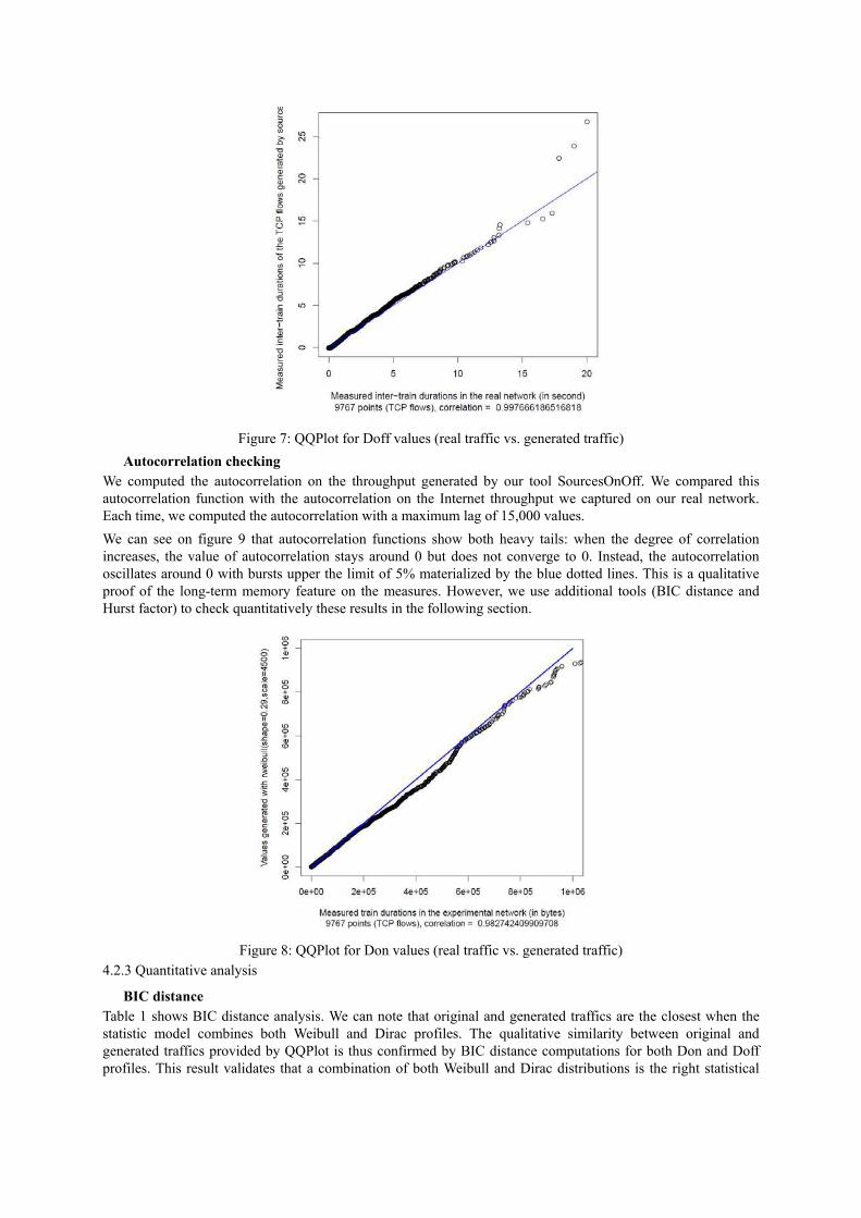
Figure 7: QQPlot for Doff values (real traffic vs. generated traffic)

Autocorrelation checking

We computed the autocorrelation on the throughput generated by our tool SourcesOnOff. We compared this

autocorrelation function with the autocorrelation on the Internet throughput we captured on our real network.

Each time, we computed the autocorrelation with a maximum lag of 15,000 values.

We can see on figure 9 that autocorrelation functions show both heavy tails: when the degree of correlation

increases, the value of autocorrelation stays around 0 but does not converge to 0. Instead, the autocorrelation

oscillates around 0 with bursts upper the limit of 5% materialized by the blue dotted lines. This is a qualitative

proof of the long-term memory feature on the measures. However, we use additional tools (BIC distance and

Hurst factor) to check quantitatively these results in the following section.

Figure 8: QQPlot for Don values (real traffic vs. generated traffic)

4.2.3 Quantitative analysis

BIC distance

Table 1 shows BIC distance analysis. We can note that original and generated traffics are the closest when the

statistic model combines both Weibull and Dirac profiles. The qualitative similarity between original and

generated traffics provided by QQPlot is thus confirmed by BIC distance computations for both Don and Doff

profiles. This result validates that a combination of both Weibull and Dirac distributions is the right statistical

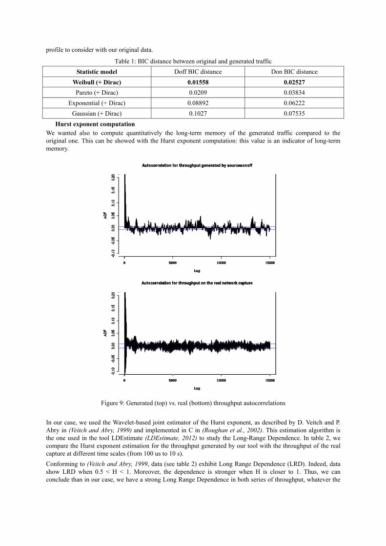
profile to consider with our original data.

Table 1: BIC distance between original and generated traffic

Statistic model Doff BIC distance Don BIC distance

Weibull (+ Dirac) 0.01558 0.02527

Pareto (+ Dirac) 0.0209 0.03834

Exponential (+ Dirac) 0.08892 0.06222

Gaussian (+ Dirac) 0.1027 0.07535

Hurst exponent computation

We wanted also to compute quantitatively the long-term memory of the generated traffic compared to the

original one. This can be showed with the Hurst exponent computation: this value is an indicator of long-term

memory.

Figure 9: Generated (top) vs. real (bottom) throughput autocorrelations

In our case, we used the Wavelet-based joint estimator of the Hurst exponent, as described by D. Veitch and P.

Abry in (Veitch and Abry, 1999) and implemented in C in (Roughan et al., 2002). This estimation algorithm is

the one used in the tool LDEstimate (LDEstimate, 2012) to study the Long-Range Dependence. In table 2, we

compare the Hurst exponent estimation for the throughput generated by our tool with the throughput of the real

capture at different time scales (from 100 us to 10 s).

Conforming to (Veitch and Abry, 1999, data (see table 2) exhibit Long Range Dependence (LRD). Indeed, data

show LRD when 0.5 < H < 1. Moreover, the dependence is stronger when H is closer to 1. Thus, we can

conclude than in our case, we have a strong Long Range Dependence in both series of throughput, whatever the

time window is defined. We can also conclude that both generated and original traffics exhibit the same LRD

level (considering a 12 % error interval).

Table 2: Hurst exponent estimations

Sample duration for

throughput

measure-ments

Hurst Exponent estimation

(H)

for our tool

SourcesOnOff

H exponent for the

real throughput

Ratio between generated

traffic and real traffic

100 us 0.88 0.83 7 %

10 ms 0.97 0.95 2 %

100 ms 1.00 1.00 0 %

1 second 1.00 0.88 12 %

10 s 1.00 1.00 0 %

5. SourcesOnOff usages

In this section, we address specific usages that we can imagine for this tool. For instance, it may be useful to

apply transformations on the traffic profile we want to generate. Thus, let us imagine an example where we have

a real data and its extracted statistic profile to be equivalent to a load of 100 users on the network. Assuming the

hypothesis “the throughput is proportional with the number of users” and “the inter-flow durations are inversely

proportional to the number of users”, we can do network provisioning with some simple mathematical operations

on the raw parameters of the profile. It is, for us, extremely harder to do the same operations with a capture of

raw packets that we would like to replay.

In this section, we will consider an example where we want “to emulate the network intensity in the case we have

now 150 users (rather the 100 users observed in the real data) but the same systems”. The goal is to be able to

predict the final throughput Y (Mbps) that we need to generate with our tool to represent the 150 users.

If the parameters of the Don and the Doff distributions are not adequate, the network throughput may differ

greatly from expected. We can do an analogy with a sinusoidal signal. As illustrated in figure 10, if the signal is

too low, the capacity will be underused, while if the signal is too much amplified, it will saturate the channel and

measures will differ from a sinus.

Figure 10: Explanation of tuning with the sinus function

With a high-capacity network infrastructure, high values for inter-train durations (Doff) and low values for

quantity of data per flow (Don), the network throughput will mostly be empty (~0% load), with bursts for each

source starting. On the contrary, with a low-capacity network infrastructure, high values for Don and low values

for Doff, the network will be soon saturated (~100% load). Then, the transmitter system may fail to create new

sources, due to not enough network resources to establish new connections, until old connections finishes.

Figure 11 illustrates the three cases of tuning: the blue line at left represents a low throughput generated by

SourcesOnOff, the black line at the center of the figure a medium throughput and the blue line at right a high

overhead where the network path is mostly saturated. Note that each of the three cases provides some

information: high throughputs enable the tester to estimate the network path capacity, low throughputs to

evaluate system behavior in front of burst and medium throughputs to evaluate system behavior to a regular and

long stress.

We can expect an average throughput of X Mbps = Don.average * (1/ Doff.average). In order to realize an

average throughput of Y Mbps instead of the current average of X Mbps, we have to adjust proportionally the

Doff average value: Doff_new_mean = (X/Y)*Doff_old_mean. In our opinion, the Don values correspond to

the behavior of the users and the Doff values is inversely proportional to the number of users. So changing the

Don parameters would make the flows unrealistic whereas the Doff average value would reduce the number of

simultaneous flows.

For some specific statistical profiles, the mean is not a characterization parameter of the distributions. For

instance, this is the case for the Weibull distributions. These distributions use mostly a “scale” parameter which

is proportional with the mean of the distribution. Thus, with Weibull distributions, we should apply the following

equation: Doff_scale_new = (Y/X)*Doff_scale_old.

If we come back to the pratical example we are considering in this section, we should do the same operation to

reach our objective “emulate the network with 150 users instead of the 100 users”. This is achieved by dividing

the Doff scale by a factor of 1.5 and thus we use a scale factor of 193 ms for the Doff Weibull distribution. This

simple example gives a overview on how this SourcesOnOff tool can be easily tuned in order to manage

different performance goals.

Figure 11: Explanation of tuning impact on SourcesOnOff

5. Conclusion and future work

In this paper, we have introduced a methodology to generate network traffic with realistic characteristics. A tool

has been developed, based on the application of ON/OFF sources with different statistical profiles. Parameters of

the distributions can be defined by the user or extracted from real traffic analysis. We have completed this paper

with a validation of both the traffic generation methodology and the SourcesOnOff tool. Different experiments

have been conducted. All of them validate that our tool is able to generate traffic with the same characteristics

than real ones.

The tool is freely available and may be utilized for a wide variety of network traffic profiles. We hope users can

appreciate the wide range of applications where SourceOnOff can be utilized. We can cite, for instance, network

provisioning, application testing or network mechanism enhancement. For this last field of application, this tool

can be useful to generate random data in order to observe bufferbloats, to stress an intermediary network system

with a big number of simultaneous flows or to generate network traffics to observe TCP race conditions.

However, additional work would have to be conducted by considering different traffic traces collected in

different points of presence of the Internet. We could imagine to have an access in the future to traffic captured

not only on the firewall of a LAN but also on a core router of the Internet. By putting our SourceOnOff tool

freely available to the research community, we hope we can provide a first level of contribution to improve

characterization results for Internet traffic understanding.

Furthermore, this tool is currently unable to generate traffic different than TCP and UDP protocols. In the future,

the tool may be completed with support for ICMP protocol or additional transport protocols such as SCTP

(Stream Control Transmission Protocol) (Stewart, 2007) for instance. Moreover, the tool may support other

statistical distribution profiles and may provide additional statistics for the users. The validation of this tool

being completed, we can now take into account more complex network topologies (cloud computing applications

for instance) and distribute different SourcesOnOff sender and receiver agents among them for the future

experiments we plan to realize.

Acknowledgements

We would like to thank Benoit Sainct (MS student) for his work in implementing some of the statistical tools

used for traffic characterization.

References

Becker R. A., Chambers J. M. & Wilks, A. R. (1988) The New S Language. Wadsworth & Brooks/Cole

BWPing (2013), Open Source bandwidth measurement tool, http://bwping.sourceforge.net/, 2013/01/21

Dreibholz T. (2011), NetPerfMeter, A TCP/UDP/SCTP/DCCP Network Performance Meter Tool,

http://www.iem.uni-due.de/~dreibh/netperfmeter/, 2012/12/21

Dumpcap (2013), Dump network traffic, http://www.wireshark.org/docs/man- pages/dumpcap.html, 2013/01/21

GCC (2013), the GNU Compiler Collection, gcc.gnu.org

Gebert S., Pries R., Schlosser D. & Heck K. (2011), Internet Access Traffic Measurement and Analysis, Univ of Würzburg,

Inst. Of Computer Sciences, Germany, Hotzone GmbH

GPLv3 (2013), Welcome to GPLv3, http://gplv3.fsf.org/, 2013/01/21

Iperf (2013), a modern alternative for measuring maximum TCP and UDP bandwidth performance,

http://iperf.sourceforge.net/,2013/01/21

IPsumDump (2013), IPsumDump and IPaggCreate website, http://www.read.seas.harvard.edu/~kohler/ipsumdump/,

2013/01/31

Karagiannis T. (2002), SELFIS: A Short Tutorial, November 8, 2002

LDestimate (2012), Code for the estimation of Scaling Exponents, website of Veitch Darryl, 2012,

http://www.cubinlab.ee.unimelb.edu.au/%7Edarryl/secondorder_code.html

Leland W. E., Taqqu S. M., Willinger W. & Wilson D. V. (1994), On the Self-Similar Nature of Ethernet Traffic, (Extended

Version) IEEE/ACM TRANSACTIONS ON NETWORKING, VOL. 2, NO. 1, FEBRUARY 1994

NetPerf (2013), The NetPerf HomePage, http://www.netperf.org/netperf/, 2013/01/21

NS-2 (2013), The Network Simulator - ns-2, http://www.isi.edu/nsnam/ns/, 2013/01/21

Olivier P. & Benameur N. (2000), Flow Level IP traffic characterization, France Télécom, 2000

OMNet++ (2013), OMNet++ Network Simulation Framework website, http://www.omnetpp.org/, 2013/01/21

Opnet (2013), The Opnet Website, http://www.opnet.com/, 2013/01/21

R (2013), The R Project for Statistical Computing, http://www.r-project.org/, 2013/01/21

RéMiP (2013), RéMiP 2000 website, http://www.remip.prd.fr, 2013/01/07

Renater (2013), Le Réseau National de télécommunications pour la Technologie l'Enseignement et la Recherche,

http://www.renater.fr/, 2013/01/07

Roughan M., Stiessel A. & Veitch D. (2002), Program in C to estimate on-line the hurst component, 2002,

http://www.cubinlab.ee.unimelb.edu.au/~darryl/On-Line_code.tar.gz, checked the 2013/01/31

Schwarz B. & Gideon E (1978), Estimating the dimension of a model, Annals of Statistics 6 (2): 461–464, 1978

Stewart, R. (2007), Stream Control Transmission Protocol, Request for Comments: 4960, September 2007

Tcpdump (2013), Tcpdump & LibPcap public repository, www.tcpdump.org, 2013/01/31

Ttcp (2010), test TCP/UDP performance, http://linux.die.net/man/1/ttcp, 2013/01/21

Varet A., Larrieu N. & Macabiau C. (2012), Design and development of an embedded aeronautical router with security

capabilities, in Proceedings of the ICNS Conference on Integrated Communications Navigation and Surveillance (Washington,

2012)

Veitch T. & Abry P. (1999), A Wavelet Based Joint Estimator of the Parameters of Long-Range Dependence, pp.878-897,

Vol.45(3), IEEE Trans. Info. Theory, special issue "Multiscale Statistical Signal Analysis and its Applications"

Willinger W., Taqqu M. S., Sherman R. & Wilson D. V. (1997), Self-Similarity Through High-Variability: Statistical Analysis

of Ethernet LAN Traffic at the Source Level, IEEE/ACM TRANSACTIONS ON NETWORKING, VOL. 5, NO. 1,

FEBRUARY 1997

Wireshark (2013), Go Deep, http://www.wireshark.org/, 2013/01/21

Notes

Note 1. Tcpreplay website: http://tcpreplay.synfin.net/

Note 2. Harpoon website: https://github.com/jsommers/harpoon

Note 3. Ostinato website : http://wiki.ostinato.googlecode

Note 4. Note that for debugging purposes, additional information may be printed by the SourcesOnOff program,

such as the TCP_INFO structure of each TCP flow just before the connection is closed.

Note 5. Quantmod website: http://quantmod.r-forge.r-project.org

Copyrights

Copyright for this article is retained by the author(s), with first publication rights granted to the journal.

This is an open-access article distributed under the terms and conditions of the Creative Commons Attribution

license (http://creativecommons.org/licenses/by/3.0/).