Embed Size (px)
Citation preview

Real-Time Trading Models and the Statistical
Properties of Foreign Exchange Rates
Ramazan Gen�cay� Giuseppe Ballocchi Michel Dacorogna
Richard Olsen Olivier Pictet
Olsen & Associates
Seefeldstrasse 233, CH-8008, Zurich, Switzerland
December 1998
JEL No: G14, C45, C52, C53
Key Words: Real-time trading models, exponential moving averages, robust kernels, technical trad-
ing.
�This paper was written while Gen�cay visited Olsen & Associates as a research scholar. He
is grateful to them for their generosity and for providing an excellent research platform for high
frequency �nance research. Gen�cay also thanks the Social Sciences and Humanities Research Coun-
cil of Canada and the Natural Sciences and Engineering Research Council of Canada for �nancial
support. Address for correspondance: Ramazan Gen�cay, Department of Economics, Mathemat-
ics and Statistics, University of Windsor, 401 Sunset Avenue, Windsor, Ontario, Canada. Email:
[email protected], Tel: (519) 253 3000 ext. 2382, Fax: (519) 973 7096.

Abstract
Real-time trading models use high frequency live data feeds and their rec-
ommendations are transmitted to the traders through data feed lines instanta-
neously. In this paper, a widely used real-time trading model is used to evaluate
the statistical properties of foreign exchange rates. The out-of-sample test pe-
riod is seven years of �ve-minute series on three major foreign exchange rates
against the US Dollar and one cross rate. Performance of the real-time trading
models is measured by the annualized return, two measures of risk corrected
annualized return, deal frequency and maximum drawdown. The simulated
probability distributions of these performance measures are calculated with the
three traditional processes, the random walk, GARCH and AR-GARCH. The
null hypothesis that the real-time performances of the foreign exchange series
are generated from these traditional processes is tested under the probability
distributions of the performance measures.
All four currencies yield postive annualized returns in the studied sampling
period. These annualized returns are net of transaction costs. The results
indicate that the excess returns of the real-time trading models, after taking
the transaction costs and correcting for market risk, are not spurious. The
results reject the random walk, GARCH(1,1) and AR-GARCH(1,1) processes
as the data generating mechanisms for the high frequency foreign exchange
rates. One important reason for the rejection of the GARCH type processes as
a data generating mechanishm of foreign exchange returns is the aggregation
property of the GARCH processes. The GARCH process behaves more like a
homoskedastic process at lower frequencies. Since the real-time trading model's
trading frequency is less than two deals per week, the trading model does not
pick up the �ve minute level heteroskedastic structure at the weekly frequency.
The results indicate that the foreign exchange series may possess a multi-
frequency conditional mean and conditional heteroskedastic dynamics. The
traditional heteroskedastic models fail to capture the entire dynamics by only
capturing a slice of this dynamics at a given frequency. Therefore, a more
realistic processes for foreign exchange returns should give consideration to the
scaling behavior of returns at di�erent frequencies and this scaling behavior
should be taken into account in the construction of a representative process.
1

1. Introduction
The foreign exchange market is the largest �nancial market worldwide which involves
dealers in di�erent geographical locations, time zones, working hours, time horizons,
home currencies, information access, transaction costs, and other institutional con-
straints. The time horizons vary from intra-day dealers, who close their positions
every evening, to long-term investors and central banks. In this highly complex
and heterogeneous market structure, the market participants are faced with di�erent
constraints and use di�erent strategies to reach their �nancial goals such as by max-
imizing their pro�ts or maximizing their utility function after adjusting for market
risk.
Real-time trading models use high frequency live data feeds and their recommen-
dations are transmitted to the traders through data feed lines instantaneously. In this
paper, a popular real-time trading model is used to evaluate the statistical properties
of foreign exchange rates. The out-of-sample test period is seven years of �ve-minute
series on three major foreign exchange rates and one cross rate. Performances of the
real-time trading models is measured by the annualized return, two measures of risk
corrected annualized return, deal frequency and maximum drawdown.
The main essence behind the real time trading models is that they are designed
to capture the conditional mean dynamics of the return process for foreign exchange
rates under changing market conditions, trading intervals, opening and closing times,
market holidays and di�erent market horizons varying from short-term to long-term
horizons. Until recently, the common ground was that the return process follows a
random walk and therefore there would be nothing in the conditional mean to capture.
The objective of this study is to examine whether the excess returns of the real-time
trading models of foreign exchange rates are obtained by pure luck or whether these
models in fact capture subtle persistence in the conditional mean dynamics of the
foreign exchange returns. The contributions of this study are twofold. The �rst
contribution involves the examination of the performance of the trading models with
traditional statistical processes such as the random walk, generalized autoregressive
conditional heteroskedastic process (GARCH) and the autoregressive GARCH (AR-
GARCH) process. The second contribution is to test whether a sophisticated trading
model has any value added over a model based on a simple technical indicator. The
null hypothesis of whether the data generating process for the foreign exchange returns
is generated from these processes is tested by comparing the performance of the actual
data under the simulated distribution of the performance measures for these processes.
2

The sensitiveness of the performance measures is also investigated with reference to
the di�erent market horizons.
The real-time trading models studied here are based on technical analysis. In
the earlier literature, simple technical indicators for the securities market have been
tested by Brock et al. (1992). Their study indicates that patterns uncovered by
technical rules cannot be explained by simple linear processes or by changing the
expected returns caused by changes in volatility. LeBaron (1992,1997) and Levich
and Thomas (1993) follow the methodology of Brock et al. (1992) and use bootstrap
simulations to demonstrate the statistical signi�cance of the technical trading rules
against well-known parametric null models of exchange rates.
In Sullivan et al. (1997), an extensive study of the trading rule performance is
examined by extending the Brock et al. (1992) data for the period of 1987-1996. The
results of Sullivan et al. (1997) indicate that the trading rule performance remains
superior for the time period that Brock et al. (1992) studied, however, these gains
disappear in the last ten years of the Dow Jones Industrial Average (DJIA) series. In
fact, Sullivan et al. (1997) report that the performance of the out-of-sample results of
the technical indicators are completely reversed and the best performing trading rule is
not even statistically signi�cant at standard critical levels for the period from 1987 to
1996. One conclusion of their paper is that their �ndings are not representative as the
results can be attributed to an unusually large one-day movement which occured on
October 1987. The other conclusion is that the technical trading rules did historically
well by producing superior performance, but that, more recently, the markets have
become more e�cient and hence such opportunities have disappeared.
In Gen�cay (1998a), the DJIA data set of Brock et al. (1992), is studied with simple
moving average indicators within the nonparametric conditional mean models. The
results indicate that nonparametric models with buy-sell signals of the moving aver-
age models provide more accurate sign and mean squared prediction errors (MSPE)
relative to a random walk and GARCH models. Gen�cay (1998b) shows that past
buy-sell signals of simple moving average rules provide statistically signi�cant sign
predictions for modelling the conditional mean of the returns for the foreign exchange
rates. The results in Gen�cay (1998b) also indicate that past buy-sell signals of the
simple moving average rules are more powerful for modelling the conditional mean
dynamics in the nonparametric models.
Overall, the scope of the most recent literature supports the technical analysis
but it is limited to simple univariate technical rules. One particular exception is
the study by Dacorogna et al. (1995) which examines real-time trading models of
3

foreign exhanges under heterogeneous trading strategies. Dacorogna et al. (1995)
point out that there is no particular trading strategy that is systematically better
than all the others at all times. Rather, excess return should be evaluated within the
context of di�erent trading pro�les and this requires various ways of evaluating risk
and return in a trading model. They also point out that the most pro�table trading
models actively trade when many agents are in the market (high liquidity) and do not
trade at other times of the day and on weekends. This pro�tability of the real-time
trading models is attributed to the simultaneous presence of heterogeneous agents
who utilize di�erent trading strategies based on their trading horizon. Therefore, it is
the identi�cation of the heterogeous market microstructure in a trading model which
leads to an excess return after adjusting for market risk.
Real-time trading models studied in Pictet et al. (1992) and Dacorogna et al.
(1995) utilize technical based information and are also available commercially through
Olsen & Associates. Olsen & Associates (O&A) has collected and analyzed large
amounts of foreign exchange quotes by market makers around the clock (up to 10000
non-equally spaced prices per day for the German Mark against the US Dollar). Based
on this data, O&A has developed a highly sophisticated set of real-time trading mod-
els. These models give explicit trading recommendations under realistic constraints
and explicitly take into account the heterogeneous structure of the foreign exchange
markets by utilizing information on opening hours of a market, di�erent time zones
and local holidays. The models1 have been running real-time for more than eight
years with intra-day data, thus providing a long period of time series data for an ex
ante test.
The period of study covers the �rst trading day in 1990 until December 31, 1996, a
period of seven years at the �ve minutes frequency. Other studies such as Sullivan et
al. (1997) found technical indicators to be ine�ective for the DJIA between 1987-1997.
Although our study focuses solely on the spot exchange markets, it will provide a
benchmark for whether a similar absence of pro�tability also prevails in spot exchange
markets in a seven year period between 1990-1996.
1Another aspect of O&A trading models is that trading recommendations transmitted to the
customers include a theoretical trading model execution price which is derived from bid/ask quotes
using conservative assumptions. The customer who executes the recommendation compares the
actual price he got with the trading model execution price. The experience of eight years of trading
model operation indicates that the theoretical trading model execution price is rather conservative,
since customers often achieve prices that are more favorable to them. This means that the actual
performance of the models is typically slightly better than what is calculated on the basis of the
theoretical trading model execution price.
4

The results of this paper indicate that:
� The four currencies pairs, USD-DEM (US Dollar-Deutsche Mark), USD-CHF
(US Dollar-Swiss Franc), USD-FRF (US Dollar-French Franc) and DEM-JPY
(Deutsche Mark-Japanese Yen) yield 9.63, 3.66, 8.20 and 6.43 percent annual-
ized returns in the studied sampling period. These annualized returns are net
of transaction costs.
� The simulated probability distributions of the performance measures are calcu-
lated with the random walk, GARCH(1,1) and AR(4)-GARCH(1,1) processes.
The null hypothesis that the real-time performances of the foreign exchange
series are generated from these traditional processes is rejected under the prob-
ability distributions of the performance measures.
� One important reason for the rejection of the GARCH(1,1) process as a data
generating mechanishm of foreign exchange returns is the aggregation property
of the GARCH(1,1) process. The high frequency GARCH(1,1) process behaves
more like a homoskedastic process at lower frequencies. Since the real-time
trading model's trading frequency is less than two deals per week, the trading
model does not pick up the �ve minute level heteroskedastic structure at the
weekly frequency. Rather, the heteroskedastic structure behaves as if it is mea-
surement noise where the model takes positions and this leads to the rejection
of the GARCH(1,1) as a data generation process of the foreign exchange series.
In a GARCH process, the conditional heteroskedasticity exists in the frequency
that the data has been generated. As it is moved away from this frequency to
lower frequencies, the heteroskedastic structure slowly dies away leaving itself
to a more homogeneous structure in time. A more elaborate processes such as
the multiple horizon ARCH models2
possess conditionally heteroskedastic structure at all frequencies in general. The
existence of multiple frequency heteroskedastic structure may be more in line
with the heterogeneous structure of the foreign exchange markets.
Similarly, one possible explanation for the rejection of the AR(4)-GARCH(1,1)
process is the relationship between the dealing frequency of the model and the
2Andersen and Bollerslev (1997) analysed the intraday periodicity and volatility persistence in
�nancial markets. They show that intraday periodicity in the return volatility in foreign exchange
markets has a strong impact on the dynamic properties of high frequency returns. M�uller et al.
(1997) designed a multiple horizon HARCH process to address the conditionally heteroskedastic
nature of the foreign exchange returns at di�erent frequencies.
5
frequency of the simulated data. The AR(4)-GARCH(1,1) process is generated
at the 5 minutes frequency but the model's dealing frequency is one or two deals
per week. Therefore, the model picks up the high frequency serial correlation
as a noise and this serial correlation works against the process. This cannot
be treated as a failure of the real-time trading model. Rather, this strong
rejection is an evidence of the failure of the aggregation properties of the AR(4)-
GARCH(1,1) process over lower frequencies.
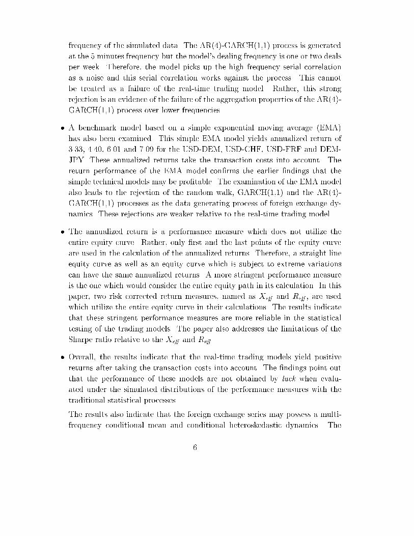
� A benchmark model based on a simple exponential moving average (EMA)
has also been examined. This simple EMA model yields annualized return of
3.33, 4.40, 6.01 and 7.09 for the USD-DEM, USD-CHF, USD-FRF and DEM-
JPY. These annualized returns take the transaction costs into account. The
return performance of the EMA model con�rms the earlier �ndings that the
simple technical models may be pro�table. The examination of the EMA model
also leads to the rejection of the random walk, GARCH(1,1) and the AR(4)-
GARCH(1,1) processes as the data generating process of foreign exchange dy-
namics. These rejections are weaker relative to the real-time trading model.
� The annualized return is a performance measure which does not utilize the
entire equity curve. Rather, only �rst and the last points of the equity curve
are used in the calculation of the annualized returns. Therefore, a straight line
equity curve as well as an equity curve which is subject to extreme variations
can have the same annualized returns. A more stringent performance measure
is the one which would consider the entire equity path in its calculation. In this
paper, two risk corrected return measures, named as Xe� and Re� , are used
which utilize the entire equity curve in their calculations. The results indicate
that these stringent performance measures are more reliable in the statistical
testing of the trading models. The paper also addresses the limitations of the
Sharpe ratio relative to the Xe� and Re� .
� Overall, the results indicate that the real-time trading models yield positive
returns after taking the transaction costs into account. The �ndings point out
that the performance of these models are not obtained by luck when evalu-
ated under the simulated distributions of the performance measures with the
traditional statistical processes.
The results also indicate that the foreign exchange series may possess a multi-
frequency conditional mean and conditional heteroskedastic dynamics. The
6

traditional heteroskedastic models fail to capture the entire dynamics by only
capturing a slice of this dynamics at a given frequency. Therefore, a more re-
alistic processes for foreign exchange returns should give consideration to the
scaling behavior of foreign exchange returns at di�erent frequencies and this
scaling behavior should be taken into account in the construction of a represen-
tative process.
The paper is organized as follows. In section two, the performance measures are
explained. The simulation models and the simulation methodology are presented in
section three. The technical indicators and their robusness properties are explained
in section four. The trading models are described in section �ve. We discuss the
empirical results in section six. We conclude afterwards.
2. Performance Measures
In this section we describe the performance measures3 used to evaluate the trading
models in this paper. The total return, RT , is a measure of the overall success of a
trading model over a period T , and de�ned by
RT �
nXj=1
rj (1)
where n is the total number of transactions during the period T and j is the jth
transaction and rj is the return from the jth transaction. The total return expresses
the amount of pro�t made by a trader always investing up to his initial capital or
credit limit in his home currency. The annualized return, �RT;A, is calculated by
multiplying the total return with the ratio of the number of days in a year to the
total number of days in the entire period.
The maximum drawdown, DT , over a certain period T = tE � t0, is de�ned by
DT � max( Rta �Rtb j t0 � ta � tb � tE ) (2)
where Rta and Rtb are the total returns of the periods from t0 to ta and tb respectively.
The trading model performance needs to account for a high total return; a smooth,
almost linear increase of the total return over time; a small clustering of losses and
no bias towards low frequency trading models. A measure frequently used by prac-
titioners to evaluate portfolio models is the Sharpe ratio. Unfortunately, the Sharpe
3The performance measures of this paper are also used in Pictet et al. (1992).
7

ratio is numerically unstable for small variances of returns and cannot consider the
clustering of pro�t and loss trades. As the basis of a risk-sensitive performance mea-
sure, a trading model return variable ~R is de�ned to be the sum of the total return
RT and the unrealized current return rc. The variable ~R re ects the additional risk
due to unrealized returns. Its change over a time interval �t is
X�t = ~Rt �~Rt��t (3)
where t expresses the time of the measurement. In this paper, �t is allowed to vary
from seven days to 301 days.
A risk-sensitive measure of trading model performance can be derived from the
utility function framework (Keeney and Rai�a (1976)). Let us assume that the vari-
able X�t follows a Gaussian random walk with mean X�t and the risk aversion
parameter � is constant with respect to X�t. The resulting utility u(X�t) of an ob-
servation is � exp(��X�t), with an expectation value of u = u(X�t) exp(�2�2�t=2),
where �2�t is the variance of X�t. The expected utility can be transformed back to
the e�ective return, Xe� = � log(�u)=� where
Xe� = X�t ���2�t
2: (4)
The risk term ��2�t=2 can be regarded as a risk premium deducted from the original
return where �2�t is computed by
�2�t =n
n� 1
�X2
�t �X2
�t
�: (5)
Unlike the Sharpe ratio, this measure is numerically stable and can di�erentiate be-
tween two trading models with a straight line behaviour (�2�t = 0) by choosing the
one with the better average return4.
The measure Xe� still depends on the size of the time interval �t. It is hard to
compareXe� values for di�erent intervals. The usual way to enable such a comparison
is through the annualization factor, A�t, where A�t is the ratio of the number of �t
in a year divided by the number of �t's in the full sample.
Xe� ;ann;�t = A�t Xe� = X ��
2A�t �
2�t (6)
where X is the annualized return and it is no longer dependent on �t. The factor
A�t�2�t has a constant expectation, independent of �t. This annualized measure still
4An example for the limitation of the Sharpe ratio is its inability to distinguish between two
straigth line equity curves with di�erent slopes.
8

has a risk term associated with �t and is insensitive to changes occurring with much
longer or much shorter horizons. To achieve a measure that simultaneously considers
a wide range of horizons, a weighted average of several Xe� ;ann is computed with
n di�erent time horizons �ti, and thus takes advantage of the fact that annualized
Xe� ;ann can be directly compared
Xe� =
Pni=1wiXe� ;ann;�tiPn
i=1wi
(7)
where the weights w are chosen according to the relative importance of the time
horizons �ti and may di�er for trading models with di�erent trading frequencies. In
this paper, � is set to � = 0:10.
The risk term of Xe� is based on the volatility of the total return curve against
time, where a steady, linear growth of the total return represents the zero volatility
case. This volatility measure of the total return curve treats positive and negative
deviations symmetrically, whereas foreign exchange dealers become more risk averse in
the loss zone and do hardly care about the clustering of positive pro�ts. A measure
which treats the negative and positive zones asymmetrically is de�ned to be Re�
(M�uller, Dacorogna and Pictet (1993)) where Re� has a high risk aversion in the zone
of negative returns and a low one in the zone of pro�ts whereas Xe� assumes constant
risk aversion. A high risk aversion in the zone of negative returns means that the
performance measure is dominated by the large drawdowns. The Re� has two risk
aversion levels: a low one, �+, for positive � ~R (pro�t intervals) and a high one, ��,
for negative � ~R (drawdowns)
� =
(�+ for � ~R � 0
��
for � ~R < 0
where �+ < ��. The high value of �
�re ects the high risk aversion of typical market
participants in the loss zone. Trading models may have some losses but, if the loss
observations strongly vary in size, the risk of very large losses becomes unacceptably
high. On the side of the positive pro�t observations, a certain regularity of pro�ts
is also better than a strong variation in size. However, this distribution of positive
returns is never vital for the future of market participant as the distribution of losses
(drawdowns). Therefore, �+ is much smaller than ��. In this paper, we assume that
�+ = ��=4 and �
�= :20.
Amongst annualized return, Xe� and Re� , the last two performance measures
examine the entire equity curve contrary to the annualized total return. The Xe�
and Re� are more stringent performance measures by taking into account the entire
9

path in the equity curve. The annualized return, on the other hand, leaves a large
degree of freedom to an in�nite number of equity curve paths by only considering the
beginning and the end points of the equity curve performance.
3. Simulation Methodology
The distributions of the performance measures under various null processes will be
calculated by using a simulation methodology. The random walk process is de�ned
by
rt = � + �t (8)
where rt = log(pt=pt�1) and �t � N(0,�2). The random walk estimation involves the
regression of the actual foreign exchange returns on a constant. A simulation sample
for the random walk series with drift is obtained by sampling from the Gaussian
random number generator with the mean and the standard deviation of the residual
series. The simulated residuals are added to the conditional mean de�ned by �̂, to
form a new series of returns. The new series of the returns has the same drift in
prices, the same variance and the same unconditional distribution. From the new
series of returns, the simulated price process is recovered recursively by setting the
initial price to the true price at the beginning of the sample. The trading models use
the bid and ask prices as inputs. Half of the average spread is subtracted (added)
from the simulated price process to obtain the simulated bid and ask prices.
The GARCH(1,1) process is written as
rt = 0 + �t (9)
where �t = h1=2t zt, zt � N(0,1) and ht = �0 + �1ht�1 + �1�
2t�1. GARCH speci�cation
(Bollerslev (1986)) allows the conditional second moments of the return process to
be serially correlated. This speci�cation implies that periods of high (low) volatility
are likely to be followed by periods of high (low) volatility. GARCH speci�cation
allows the volatility to change over time and the expected returns are a function of
past returns as well as volatility. The parameters and the normalized residuals are
estimated from the foreign exchange returns using the maximum likelihood procedure.
The simulated returns for the GARCH(1,1) process are generated from the simulated
normalized residuals and the estimated parameters.
10
The AR(p)-GARCH(1,1) process is written as
rt = +pX
i=1
irt�i + �t (10)
where �t = h1=2t zt zt � N(0,1) and ht = �0+�1ht�1+�1�
2t�1. The estimated parameters
of the AR(p)-GARCH(1,1) processes together with the simulated residuals are used
to generate the simulated returns from these processes. As before, half of the average
spread is subtracted (added) from the simulated price process to obtain the simulated
bid (ask) prices.
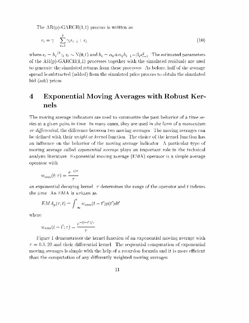
4. Exponential Moving Averages with Robust Ker-
nels
The moving average indicators are used to summarize the past behavior of a time se-
ries at a given point in time. In many cases, they are used in the form of a momentum
or di�erential, the di�erence between two moving averages. The moving averages can
be de�ned with their weight or kernel function. The choice of the kernel function has
an in uence on the behavior of the moving average indicator. A particular type of
moving average called exponential average plays an important role in the technical
analysis literature. Exponential moving average (EMA) operator is a simple average
operator with
wema(t; �) =e�t=�
�
an exponential decaying kernel. � determines the range of the operator and t indexes
the time. An EMA is written as
EMAp(�; t) =
Z t
�1
wema(t� t0)p(t0)dt0
where
wema(t� t0; �) =e�(t�t
0)=�
�
Figure 1 demonstrates the kernel function of an exponential moving average with
� = 0:5; 20 and their di�erential kernel. The sequential computation of exponential
moving averages is simple with the help of a recursion formula and it is more e�cient
than the computation of any di�erently weighted moving averages.
11

This basic exponential average kernel can be iterated to provide a family of iterated
exponential moving average kernels (M�uller (1989, 1991), Zumbach (1998))
wiema(t; �; n) =1
(n� 1)!
e�t=�
�(t=�)n�1
As n gets larger the more weight is allocated towards the middle range of the
kernel. In the limit as n goes to in�nity, the iterated exponential average behaves
like a bell-shaped curve. This implies that the center of the weight is placed in the
middle range of the kernel rather than the most recent past. For instance, a second
iterative EMA, EMA2 is written as
EMA2p(�; t) =
Z t
�1
(t� t0)
�wema(t� t0)p(t0)dt0
where
wema(t� t0; �) =e�(t�t
0)=�
�
In general, an n iterative EMA, EMAn is written as
EMAnp (�; t) =
1
(n� 1)!
Z t
�1
(t� t0)n�1
�n�1wema(t� t0)p(t0)dt0:
where
wema(t� t0; �) =e�(t�t
0)=�
�
In Figure 2, The iterative moving averages for n = 1; 2 and n = 4 are plotted which
indicate that as n gets larger the center of the weight distribution moves to the
middle part of the kernel function. A simple arithmetic moving average of length
m has a rectengular kernel which makes it very sensitive to the observations leaving
the average when the average moves over time. A more robust class of kernels which
remedy this sensitivity are the ones which assign an exponentally decaying weights to
the observations in the more distant past. These class of robust kernels are obtained
from the simple arithmetic average of the iterated exponential average kernels
wma(t; �; n) = (1=n)nX
j=1
wiema(t; �0; j) (11)
where � 0 = 2�=(n+1) so that the range, r, is independent of n. The robust exponential
moving average is written as
MAnp (�; t) =
Z t
�1
wma(t� t0; �; n)p(t0)dt0 (12)
12

This is a special case where all weights assigned to each iterative kernel is the same
in equation (11). Examples of these robust kernels are presented in Figure 3 where
equally weighted iterative exponential moving average kernels are plotted up to n =
8. The property of this kernel is that its kernel function has a plateau before it
asymptotically declines to zero. This kernel has the property that it is robust against
the exteme variations leaving the average by assigning expontially decaying weights.
It has also the property that it assigns relatively uniform weights to the most recent
history where a simple exponential average would be very sensitive to such a new
information. Therefore, a robust kernel has the property that it preserves only the
desirable robustness properties of the simple average and exponential average kernels
but ignores their highly noisy unrobust properties. In Figure 4, a robust di�erential
kernel is presented which is based on the di�erence between the exponential moving
average with � = 1 and a robust kernel with wma(� = 1; n = 8). By construction, the
area under the kernel sums to zero. The di�erential kernel assigns positive weights
to the recent past and negative weights to the distant past. The real-time trading
model of this paper uses a similar robust di�erential kernel in the construction of the
gearing function.
5. Trading Models
A distinction should be made between a price change forecast and an actual trad-
ing recommendation. A trading recommendation naturally includes a price change
forecast, but it must also account for the speci�c constraints of the dealer of the
respective trading model because a trading model is constrained by its past trading
history and the positions to which it is committed. A price forecasting model, on
the other hand, is not limited to similar types of constraints. A trading model thus
goes beyond predicting a price change such that it must decide if and at what time a
certain action has to be taken.
Trading models o�er a real-time analysis of foreign exchange movements and gen-
erate explicit trading recommendations. These models are based on the continuous
collection and treatment of foreign exchange quotes by market makers around the
clock at the tick-by-tick frequency level. There are three important reasons to utilize
high frequency data in the real-time trading models. The �rst one is that the model
indicators acquire robustness by utilizing the intraday volatility behavior in their
build-up. The second reason is that any position taken by the model may need to be
reversed quickly although these position reversals may not need to be observed often.
13

The stop-loss objectives need to satis�ed and the high frequency data provides an
appropriate platform for this requirement. More importantly, the customer's trading
positions and strategies within a trading model can only be replicated with a high
statistical degree of accuracy by utilizing high frequency data in a real-time trading
model.
The trading models imitate the trading conditions of the real foreign exchange
market as closely as possible. They do not deal directly but instead instruct human
foreign exchange dealers to make speci�c trades. In order to imitate real-world trading
accurately, they take transaction costs into account in their return computation, they
do not trade outside market working hours except for executing stop-loss and they
avoid trading too frequently. In short, these models act realistically in a manner
which a human dealer can easily follow.
Every trading model is associated with a local market that is identi�ed with a
corresponding geographical region. In turn, this is associated with generally accepted
o�ce hours and public holidays. The local market is de�ned to be open at any time
during o�ce hours provided it is neither a weekend nor a public holiday. The O&A
trading models presently support the Zurich, London, Frankfurt, Vienna and New
York markets. Typical opening hours for a model are between 8:00 and 17:30 local
time, the exact times depending on the particular local market.
The central part of a trading model is the analysis of the past price movements
which are summarized within a trading model in terms of indicators. The indicators
are then mapped into actual trading positions by applying various rules. For instance,
a model may enter a long position if an indicator exceeds a certain threshold. Other
rules determine whether a deal may be made at all. Among various factors, these
rules determine the timing of the recommendation. A trading model thus consists
of a set of indicator computations combined with a collection of rules. The former
are functions of the price history. The latter determine the applicability of the in-
dicator computations to generating trading recommendations. The model gives a
recommendation not only for the direction but also for the amount of the exposure.
The possible exposures (gearings) are �12, �1 or 0 (no exposure).
5.1. The Real Time Trading (RTT) Model
The real-time trading model studied in this paper is classi�ed as a one-horizon, high
risk/high return model. The RTT is a trend-following model and takes positions when
an indicator crosses a threshold. The indicator is a momentum based on specially
14

weighted moving averages with repeated application of the exponential moving aver-
age operator. In case of extreme foreign exchange movements, however, the model
adopts an overbought/oversold (contrarian) behaviour and recommends taking a po-
sition against the current trend. The contrarian strategy is governed by rules that
take the recent trading history of the model into account. The RTT model goes
neutral only to save pro�ts or when a stop-loss is reached. Its pro�t objective is typ-
ically at three percent. When this objective is reached, a gliding stop-loss prevents
the model from losing a large part of the pro�t already made by triggering its going
neutral when the market reverses. The gearing function for the RTT is
g(Ip) = sign(Ip) f(jIpj) c(I)
where
Ip = p�MA4p(� = 20)
where p is the logarithmic price and
f(jIpj) =
8><>:
if jIpj > b 1
if a < jIpj < b 0:5
if jIpj < a 0
and
c(I) =
(+1 if jIpj < d
�1 if jIpj > d
where a < b < d. f(jIpj) measure the size of the signal and c(jIpj) acts as a
contrarian strategy. a and b are functions of current position, volatility and trading
frequency. d is a function of position in, previous position in, sign of the the return of
the previous position. Since Xe� and Re� are implicit functions of the gearing func-
tion, the optimization of the RTT model is based on the Xe� and Re� performance.
The model is subject to the open-close and holiday closing hours. The model has
maximum stop-loss and maximum gain limits set by the environment.
5.2. A Simple Exponential Average (EMA) Model
The EMA model indicator is momentum based indicator consisting of a di�erence
between two exponential moving averages of range � = 0:5 and � = 20 days. The
gearing function for the EMA model is
g(Ip) = sign(Ip) f(jIpj)
15

where
Ip = EMA(� = 0:5)� EMA(� = 20)
and
f(jIpj) =
(if jIpj > a 1
if jIpj < a 0
where a > 0. The model is subject to the open-close and holiday closing hours. The
model has maximum stop-loss and pro�t objective which are set to the same values
as in the RTT model.
6. Empirical Results
Imitating the real world requires a system that collects all available price quotes and
reacts to each foreign exchange rate movements in real time. For the trading models,
O&A have mainly used Reuters data, but other high frequency data suppliers provide
similar information in their foreign exchange quotes. Using propriatory data �lter-
ing methods, the data is collected, validated and stored for real-time trading model
performance evaluation. The current tick frequency is approximately 10000 ticks per
business day for Deutsche Mark (USD-DEM); approximately 5000 for the other major
rates5). Altogether, the O&A database currently contains more than 16 million ticks
for USD-DEM.
The data is the �ve minutes6 #-time series from January, 1, 1990 to December,
31 1996 for the three major foreign exhange rates, USD-DEM, USD-CHF (Swiss
Franc), USD-FRF (French Franc), and the cross-rate DEM-JPY (Deutsche Mark -
Japanese Yen). The high frequency data inherits intra-day seasonalities and requires
deseasonalization. This paper uses the deseasonalization methodology advocated in
Dacorogna et al. (1993) named as the #-time seasonality correction method. The
#-time method uses the business time scale and utilizes the average volatility to rep-
resents the activity of the market. The #-time method is based on three geographical
5The abbreviations used here are de�ned by the International Organization for Standardization
(code 4217).6The real-time system uses tick-by-tick data for its trading recommendations. The historical real-
izations and the simulations in this paper are carried out with 5 minute data as it is computationally
expensive to use the tick-by-tick data for the simulations. Although, the data frequency used in this
paper is slighly lower, the historical performance of the currency pairs from the 5 minute series are
exactly compatible with performance of the real-time trading model which utilize the tick-by-tick
data.
16

markets namely the East Asia, Europe and the North America. A more detailed
exposition of the # methodology is presented in Dacorogna et al. (1993.)
The optimization and the validation of the trading models are done with data
prior to January 1, 1990. Therefore, our results here provide a complete ex-ante
test for the trading performance measures under the studied processes with seven
years of 5 minute frequency data. The simulations for each process are done for 1000
replications.
6.1. Random Walk Process
6.1.1 Real Time Trading (RTT) Model
The simulations for the RTT model are reported in Tables 1 to 4. The �rst and the
second columns are the historical realization and the p-value of the corresponding
performance measures. The p-value7 represents the fraction of simulations generating
a performance measure larger than the original. The remaining columns report the
5th and the 95th percentiles, mean, standard deviation, skewness and the kurtosis of
the simulations.
The methodology of this paper places a historical realization in the simulated
distribution of the performance measure under the assumed process and calculates its
p-value. This tells us whether the historical realization is likely to be generated from
this particular distribution or not. More importantly, it would tell if the historical
performance is likely occur in the future. A small p-value (less than 5 percent)
indicates that the historical performance lies in the right tail (or the left tail) and the
studied performance distribution is not representative of the data generating process
assuming that the trading model is a good one. If the process which generated
the performance distribution is close to the data generating process of the foreign
exchange returns, the historical performance would lie within two standard deviations
7The p-value represents a decreasing index of the reliability of a result. The higher the p-value,
the less we can believe that the observed relation between variables in the samples is a reliable
indicator of the relation between the respective variables in the population. Speci�cally, the p-value
represents the probability of error that is involved in accepting our observed result as valid, that
is, as representative of the population. For example, the p-value of 0.05 indicates that there is a 5
percent probability that the relation between the variables found in our sample is a uke. In other
words, assuming that in the population there was no relation between those variables whatsoever,
and by repeating the experiment, we could expect that approximately every 20 replications of the
experiment there would be one in which the relation between the variables in question would be
equal or stronger than ours. In many areas of research, the p-value of 5 percent is treated as a
borderline acceptable level.
17

of the performance distribution indicating that the studied process may be retained
as the representative of the data generating process.
After the transaction costs, actual data with the USD-DEM, USD-CHF, USD-
FRF and DEM-JPY yield an annualized total return of 9.63, 3.66, 8.20 and 6.43
percent, respectively. The USD-CHF has the weakest performance relative to the
other three currencies. The Xe� and Re� performance of the USD-DEM, USD-FRF
and DEM-JPY are all positive and range between 3-4 percent. For the USD-CHF, the
Xe� and Re� are -1.68 and -4.23 percent re ecting the weakness of its performance.
The p-values of the annualized return for the USD-DEM, USD-CHF, USD-FRF
and DEM-JPY are 0.3, 8.9, 1.2 and 2.1 percent, respectively. For the USD-DEM and
USD-FRF, the p-values are less than 2 percent level and it is about 2 percent for the
USD-CHF. In the case of the USD-CHF, the p-value for the annualized return is 8.9
which is well above the 5 percent level. As indicated in section 2, the annualized only
utilizes two points of the equity curve leaving a large degrees of freedom to in�nitely
many equity curves which would be compatible for a given total return. Xe� and
Re� are more stringent performance measures which utilize the entire equity curve in
their calculations. The p-values of Xe� and Re� are 0.0, 0.0 percent for USD-DEM;
0.7 and 0.6 percent for USD-CHF; 0.2 and 0.1 percent for USD-FRF and 0.2 and 0.1
percent for DEM-JPY. The p-values for the Xe� and Re� are all less than one percent
rejecting the null hypothesis that the random walk is the data generating process of
exchange rate returns.
The maximum drawdowns for the USD-DEM, USD-CHF, USD-FRF and DEM-
JPY are 11.02, 16.08, 11.36 and 12.03 percent. The mean maximum drawdowns from
the simulated random walk processes are 53.79, 63.68, 47.68 and 53.49 for the USD-
DEM, USD-CHF, USD-FRF and DEM-JPY, respectively. The mean of the simulated
maximum drawdowns are three or four times larger than the actual maximum draw-
downs. The deal frequencies are 1.68, 1.29, 1.05, 2.14 per week for the four currency
pairs from the actual data. The deal frequencies indicate that the RTT model trades
on average no more than 2 trades per week although the data feed is at the 5 minute
frequency. The mean simulated deal frequencies are 2.46, 1.98, 1.65 and 3.08 which
are signi�cantly larger than the actual drawdowns.
The values for the maximum drawdown and the deal frequency indicate that the
random walk simulation yield larger maximum drawdown and deal frequency values
relative to the values of these statistics from the actual data. In other words, the ran-
dom walk simulations deal more frequently and result in more volatile equity curves
on the average relative to the equity curve from the actual data. Correspondingly,
18

the p-values indicate that the random walk process cannot be the representative of
the actual foreign exchange series under these two performance measures. The sum-
mary statistics of the simulated performance measures have negligible skewness and
statistically insigni�cant excess kurtosis. This indicates that the distribution of the
performance measures are symmetric and do not exhibit tick tails.
The means of the simulations indicate that the distributions are correctly centered
at the average transaction costs which is expected under the random walk process.
For instance, the mean simulated deal frequency of the USD-DEM is 2.46 deals per
week or 127.92 (2:46� 52) deals per year. The percentage spread for the USD-DEM
is 0.00025 which in turn indicate an average transaction cost of -3.20. Given that
the mean of the simulated annualized return is -3.44, we can conclude that the mean
of simulated annualized return distribution is centered around the mean transaction
cost.
The behavior of the performance measures across 7 day, 29 day, 117 day and
301 day horizons are also investigated with Xe� and Re� . The importance of the
performance analysis at various horizons is that it permits a more detailed analysis
of the equity curve at the predetermined points in time. These horizons correspond
approximately to a week, a month, four months and a year's performance. The Xe�
and Re� values indicate that the RTT model's performance improves over longer time
horizons. This is in accordance with the low dealing frequency of the RTT model.
In all horizons, the p values for the Xe� and Re� are less than a half percent for
USD-DEM, USD-FRF and DEM-JPY. For USD-CHF, the p-values are less than 2.4
percent for all horizons. Overall, the multi-horizon analysis indicate the rejection of
the random walk process as a candidate for the foreign exchange returns.
6.1.2 Exponential Moving Average (EMA) Model
The simulation results for the EMAmodel are presented in Tables 5-8. The annualized
returns for the USD-DEM, USD-CHF, USD-FRF and DEM-JPY are 3.33, 4.40, 6.01
and 7.09 percent, respectively. Relative to the annualized return performance of the
RTT model, the EMA model's return performance is lower for the USD-DEM and
the USD-FRF. On the other hand, the annualized returns of the EMA model for
USD-CHF and DEM-JPY are slighly higher. One noticeable di�erence is that the
EMA model has higher maximum drawdowns for all four currency pairs relative to
the RTT model. The EMA model has also a smaller deal frequency relative to the
RTT model. The reason for the di�erence between the deal frequencies between the
two models is that the RTT model has a contrarian strategy whereas the EMA model
19

does not. The second reason is that the long indicator of the RTT model is 16 days
wheras the EMA model has a long indicator of 20 days. A relatively longer average
lets the EMA model to engage lower number of deals.
The p-values for the annualized returns are 12.6, 8.8, 6.4 and 6.6 percent for
the four currencies pairs. All four p-values are greater than the 5 percent level of
con�dence. Therefore, it is not possible to reject the null hypothesis that the data
generating process is random walk with the EMA model under the simulated annu-
alized return distributions. The examination of the p-values for the Xe� and Re�
indicate that these values are 2.8 and 2.3 percent for the USD-DEM; 0.9 and 0.4
percent for the USD-CHF; 0.6 and 0.4 percent for the USD-FRF and 1.4 and 1.0
percent for the DEM-JPY. Under these more stringent performance measure, the
null hypothesis that the random walk process is the data generating process for the
foreign exchange returns is rejected.
The p-values for the maximum drawdown and the deal frequency indicate that
the EMA model's historical performance stays well below the ones generated under
the random walk simulations. In other words, the random walk simulations always
generate larger drawdowns relative to the historical drawdowns from the four currency
pairs. In fact, the mean simulated drawdowns for the USD-DEM, USD-CHF, USD-
FRF and DEM-JPY are 49.70, 60.72, 47.51 and 44.28 percent which are at least three
times larger than the historical drawdowns. Similarly, the mean of the simulated deal
frequencies for the random walk process stays approximately 20 percent above the
historical realizations. The multi-horizon analysis of the EMA model indicate that
the model's performance improves in longer horizons. This is mostly due to the low
dealing frequency. The p-values of the four currency pairs for Xe� and Re� remain
less than 3.3 percent for the 301 day horizon.
The overall evaluation of the EMA model is that this simple technical model
generate net positive returns for all currencies after taking the transaction costs into
account. The simulated probability distributions of the performance measures also
indicate that the null hypothesis of whether the foreign exchange returns can be
characterized by random walk process is rejected. Both the RTT model as well
the EMA model are able to generate positive annualized returns (after taking the
transaction costs into account)and the performance of the RTT model is superior to
the EMA model with higher returns and smaller drawdowns. The EMA model has
smaller deal frequency per week relative to the RTT model.
20

6.2. GARCH(1,1) Process
A more realistic process for the foreign exchange returns is the GARCH(1,1) process
which allows for conditional heterskedasticity. The GARCH(1,1) estimation results
are presented in Table 9. The numbers in parantheses are the robust standard errors
and the GARCH(1,1) parameters are statistically signi�cant at the 5 percent level
for all currency pairs. The Ljung-Box statistic is calculated up to 12 lags for the
standardized residuals and it is distributed with �2 with 12 degrees of freedom. The
Ljung-Box statistic indicate no serial correlation for the USD-DEM and USD-FRF
but the USD-FRF and DEM-JPY remains serially correlated. The variance of the
normalized residuals are near one. There is no evidence of skewness but the excess
kurtosis remains large for the residuals.
6.2.1 Real Time Trading (RTT) Model
In Tables 10-13, the RTT model simulations with the GARCH(1,1) process are pre-
sented. Since GARCH(1,1) allows for conditional heteroskedasticity, it is expected
that the simulated performance of the RTT model would yield higher p-values and
therefore leading to the failure of rejection of the null hypothesis that GARCH(1,1) is
the data generating mechanishm for the foreign exchange returns. The results how-
ever indicate smaller p-values which is in favor of a stronger rejection of this process
relative to the random walk process.
One important reason for the rejection of the GARCH(1,1) process as a data
generating mechanishm of foreign exchange returns is the aggregation property of the
GARCH(1,1) process8. The GARCH(1,1) process behaves more like a homoskedastic
process as the frequency is reduced from high to low frequency. Since the RTT model's
trading frequency is less than two deals per week, the trading model does not pick up
the �ve minute level heteroskedastic structure at the weekly frequency. Rather, the
heteroskedastic structure behaves as if it is measurement noise where the model takes
positions and this leads to the stronger rejection of the GARCH(1,1) as a candidate
for the foreign exchange data generating mechanism.
In a GARCH process, the conditional heteroskedasticity exists in the frequency
that the data has been generated. As it is moved away from this frequency to lower
8Guillaume (1995) show that the use of an alternative time scale can eliminate the ine�ciencies in
the estimation of a GARCH model caused by intra-daily seasonal patterns. However, the temporal
aggregation properties of the GARCH models do not hold at the intra-daily frequencies, revealing
the presence of several time-horizon components.
21

frequencies, the heteroskedastic structure slowly dies away leaving itself to a more
homogeneous structure in time. A more elaborate processes such as the multiple
horizon ARCH models (as in the HARCH process of M�uller et al. (1997)) possess
conditionally heteroskedastic structure at all frequencies in general. The existence
of multiple frequency heteroskedastic structure seem to be more in line with the
heterogeneous structure of the foreign exchange markets.
The p-values of the annualized return for the USD-DEM, USD-CHF, USD-FRF
and DEM-JPY are 0.4, 8.4, 0.9 and 0.9 percent, respectively. All four currency pairs
except USD-CHF yield p-values which are less than one percent. The Xe� and Re�
are 0.1 and 0.0 percent for USD-DEM; 1.4 and 0.9 percent for USD-CHF; 0.1 and 0.1
percent for USD-FRF and 0.4 and 0.4 percent for DEM-JPY.
The historical maximum drawdown and deal frequency of the RTT model is small
relative to the ones generated from the simulated data. The maximum drawdowns
for the USD-DEM, USD-CHF, USD-FRF and DEM-JPY are 11.02, 16.08, 11.36 and
12.03 for the four currencies. The mean simulated drawdowns are 53.33, 60.58, 46.00
and 48.77 for the four currencies. The mean simulated maximum drawdowns are
three or four times larger than the historical ones. The historical deal frequencies are
1.68, 1.29, 1.05 and 2.14. The mean simulated deal frequencies are 2.39, 1.87, 1.59
and 2.66 for the four currencies. The di�erence between the historical deal frequencies
and the mean simulated deal frequencies remain large. Therefore, the examination
of the GARCH(1,1) process with the maximum drawdown and the deal frequency
indicate that the historical realizations of these two measures stay outside of the 5
percent level of simulated distributions of these two performance measures.
The mean simulated deal frequency for the USD-DEM is 2.39 trade per week. In
annual terms, this is approximately 124.28 deals per year. The half spread for the
USD-DEM series is about 0.00025 and this yield 3.10 percent when multiplied with
the number of deals per year. The -3.10 percent would be the annual transaction cost
of the model. For the model to be pro�table, it should yield more than 3.10 per year.
Table 10 indicates that the RTT model generates an excess annual return of 9.63
percent whereas the mean of the annualized return from the GARCH(1,1) process
stay at the -3.27 percent level.
The multi-horizon examination of the equity curve with the Xe� and Re� perfor-
mance measures indicate that the GARCH(1,1) process as a candidate for the data
generation mechanism is strongly rejected at all horizons from seven horizon to a
horizon as long as 301 days.
22

6.2.2 Exponential Moving Average (EMA) Model
The simulation performance of the EMA model under the GARCH(1,1) process is
presented in Tables 14-17. The p-values for the annualized returns for the for currency
pairs are 14.1, 9.6, 4.6 and 2.8 percent, respectively. Based on the annualized return
performance, the null hypothesis that the GARCH(1,1) process is the data generating
process of foreign exchange returns cannot be rejected for the USD-DEM and USD-
CHF. The other currency pairs stay below the 5 percent level but relatively close to
the 5 percent level providing a weak level of con�dence. In comparison with the RTT
model, the p-values of the EMM model substantially higher indicating the relative
weakness of this model as a model of foreign exchange dynamics.
The p-values of the Xe� and Re� are 2.3, 1.8 percent for USD-DEM; 0.7, 0.5
percent for USD-CHF; 0.6, 0.4 percent for USD-FRF and 0.5, 0.2 percent for the
DEM-JPY. Relative to the annualized return performance, the p-values of the Xe�
and Re� remain statistically signi�cant as the largest values is not greater than 2.3
percent. As indicated earlier, the annualized return is a performance measure does
not utilize the entire equity curve. Rather, only �rst and the last points of the equity
curve are used in the calculation of the annualized returns. Therefore, a straight line
equity curve as well as an equity curve which is subject to extreme variations can
have the same annualized returns. Based on the Xe� and Re� p-values, it can be
concluded that the GARCH(1,1) process be rejected as a data generating mechanism
of foreign exchange returns with the EMA model. The �nding of the EMA model is
line with the earlier literature, such as Brock et. al (1989), who also obtained similar
�ndings.
6.3. AR(4)-GARCH(1,1) Process
A further direction is to investigate whether a conditional mean dynamics with
GARCH(1,1) innovations would be a more successful characterization of the dynamics
of the high frequency foreign exchange returns. The conditional mean of the foreign
exchange returns are estimated with four lags of these returns. The additional lags
did not lead to substantial increases in the likelihood value. The results of the AR(4)-
GARCH(1,1) are presented in Table 18. The numbers in parantheses are the robust
standard errors and all four lags are statistically signi�cant at the 5 percent level. The
negative autocorrelation is large and higly signi�cant for the �rst lag of the returns.
This is consistent with the high frequency behavior of the foreign exchange returns
and is also observed in Dacorogna (1993). The Ljung-Box statistic indicate no serial
23
correlation in the normalized residuals. The variance of the normalized residuals are
near one. There is no evidence of skewness but the excess kurtosis remains large for
the residuals.
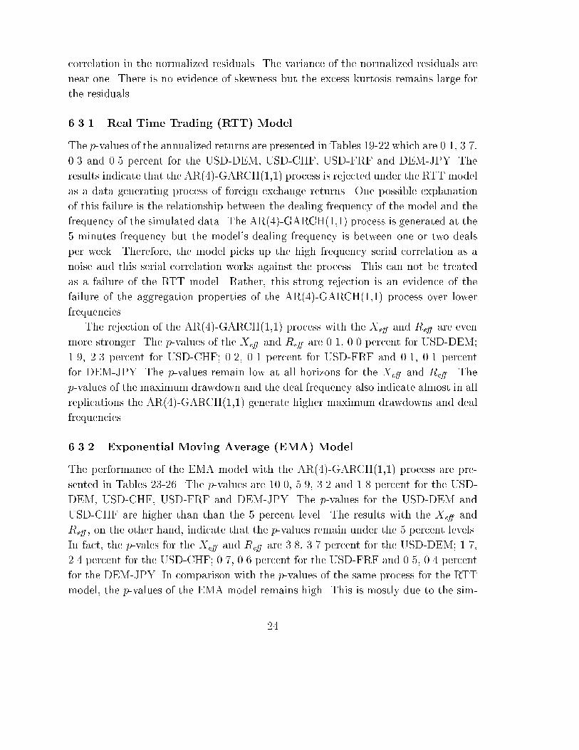
6.3.1 Real Time Trading (RTT) Model
The p-values of the annualized returns are presented in Tables 19-22 which are 0.1, 3.7,
0.3 and 0.5 percent for the USD-DEM, USD-CHF, USD-FRF and DEM-JPY. The
results indicate that the AR(4)-GARCH(1,1) process is rejected under the RTT model
as a data generating process of foreign exchange returns. One possible explanation
of this failure is the relationship between the dealing frequency of the model and the
frequency of the simulated data. The AR(4)-GARCH(1,1) process is generated at the
5 minutes frequency but the model's dealing frequency is between one or two deals
per week. Therefore, the model picks up the high frequency serial correlation as a
noise and this serial correlation works against the process. This can not be treated
as a failure of the RTT model. Rather, this strong rejection is an evidence of the
failure of the aggregation properties of the AR(4)-GARCH(1,1) process over lower
frequencies.
The rejection of the AR(4)-GARCH(1,1) process with the Xe� and Re� are even
more stronger. The p-values of the Xe� and Re� are 0.1, 0.0 percent for USD-DEM;
1.9, 2.3 percent for USD-CHF; 0.2, 0.1 percent for USD-FRF and 0.1, 0.1 percent
for DEM-JPY. The p-values remain low at all horizons for the Xe� and Re� . The
p-values of the maximum drawdown and the deal frequency also indicate almost in all
replications the AR(4)-GARCH(1,1) generate higher maximum drawdowns and deal
frequencies.
6.3.2 Exponential Moving Average (EMA) Model
The performance of the EMA model with the AR(4)-GARCH(1,1) process are pre-
sented in Tables 23-26. The p-values are 10.0, 5.9, 3.2 and 1.8 percent for the USD-
DEM, USD-CHF, USD-FRF and DEM-JPY. The p-values for the USD-DEM and
USD-CHF are higher than than the 5 percent level. The results with the Xe� and
Re� , on the other hand, indicate that the p-values remain under the 5 percent levels.
In fact, the p-vales for the Xe� and Re� are 3.8, 3.7 percent for the USD-DEM; 1.7,
2.4 percent for the USD-CHF; 0.7, 0.6 percent for the USD-FRF and 0.5, 0.4 percent
for the DEM-JPY. In comparison with the p-values of the same process for the RTT
model, the p-values of the EMA model remains high. This is mostly due to the sim-
24
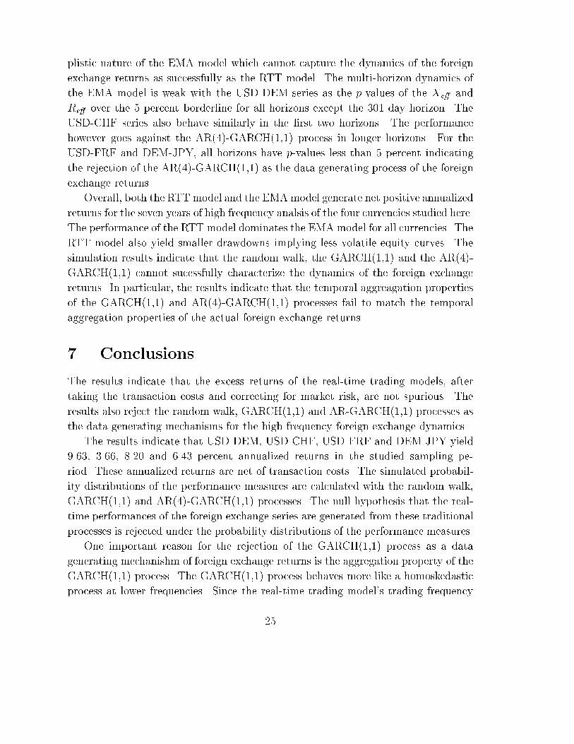
plistic nature of the EMA model which cannot capture the dynamics of the foreign
exchange returns as successfully as the RTT model. The multi-horizon dynamics of
the EMA model is weak with the USD-DEM series as the p-values of the Xe� and
Re� over the 5 percent borderline for all horizons except the 301 day horizon. The
USD-CHF series also behave similarly in the �rst two horizons. The performance
however goes against the AR(4)-GARCH(1,1) process in longer horizons. For the
USD-FRF and DEM-JPY, all horizons have p-values less than 5 percent indicating
the rejection of the AR(4)-GARCH(1,1) as the data generating process of the foreign
exchange returns.
Overall, both the RTT model and the EMAmodel generate net positive annualized
returns for the seven years of high frequency analsis of the four currencies studied here.
The performance of the RTT model dominates the EMA model for all currencies. The
RTT model also yield smaller drawdowns implying less volatile equity curves. The
simulation results indicate that the random walk, the GARCH(1,1) and the AR(4)-
GARCH(1,1) cannot sucessfully characterize the dynamics of the foreign exchange
returns. In particular, the results indicate that the temporal aggreagation properties
of the GARCH(1,1) and AR(4)-GARCH(1,1) processes fail to match the temporal
aggregation properties of the actual foreign exchange returns.
7. Conclusions
The results indicate that the excess returns of the real-time trading models, after
taking the transaction costs and correcting for market risk, are not spurious. The
results also reject the random walk, GARCH(1,1) and AR-GARCH(1,1) processes as
the data generating mechanisms for the high frequency foreign exchange dynamics.
The results indicate that USD-DEM, USD-CHF, USD-FRF and DEM-JPY yield
9.63, 3.66, 8.20 and 6.43 percent annualized returns in the studied sampling pe-
riod. These annualized returns are net of transaction costs. The simulated probabil-
ity distributions of the performance measures are calculated with the random walk,
GARCH(1,1) and AR(4)-GARCH(1,1) processes. The null hypothesis that the real-
time performances of the foreign exchange series are generated from these traditional
processes is rejected under the probability distributions of the performance measures.
One important reason for the rejection of the GARCH(1,1) process as a data
generating mechanishm of foreign exchange returns is the aggregation property of the
GARCH(1,1) process. The GARCH(1,1) process behaves more like a homoskedastic
process at lower frequencies. Since the real-time trading model's trading frequency
25

is less than two deals per week, the trading model does not pick up the �ve minute
level heteroskedastic structure at the weekly frequency. Rather, the heteroskedastic
structure behaves as if it is measurement noise where the model takes positions and
this leads to the rejection of the GARCH(1,1) as a data generation process of the
foreign exchange series.
In a GARCH process, the conditional heteroskedasticity exists in the frequency
that the data has been generated. As it is moved away from this frequency to lower
frequencies, the heteroskedastic structure slowly dies away leaving itself to a more
homogeneous structure in time. A more elaborate processes such as the multiple
horizon ARCH models possess conditionally heteroskedastic structure at all frequen-
cies in general. The existence of multiple frequency heteroskedastic structure may be
more in line with the heterogeneous structure of the foreign exchange markets.
Similarly, one possible explanation for the rejection of the AR(4)-GARCH(1,1)
process is the relationship between the dealing frequency of the model and the fre-
quency of the simulated data. The AR(4)-GARCH(1,1) process is generated at the
5 minutes frequency but the model's dealing frequency is one or two deals per week.
Therefore, the model picks up the high frequency serial correlation as a noise and this
serial correlation works against the process. This can not be treated as a failure of the
real-time trading model. Rather, this strong rejection is an evidence of the failure of
the aggregation properties of the AR(4)-GARCH(1,1) process over lower frequencies.
A benchmark model based on a simple exponential moving average (EMA) has also
been examined. This simple EMA model yields annualized return of 3.33, 4.40, 6.01
and 7.09 for the USD-DEM, USD-CHF, USD-FRF and DEM-JPY. These annualized
returns take the transaction costs into account. The return performance of the EMA
model con�rms the earlier �ndings that the simple technical models may be pro�table.
The examination of the EMA model also leads to the rejection of the random walk,
GARCH(1,1) and the AR(4)-GARCH(1,1) processes as the data generating process
of foreign exchange dynamics. These rejections are weaker relative to the real-time
trading model.
The annualized return is a performance measure which does not utilize the entire
equity curve. Rather, only �rst and the last points of the equity curve are used in
the calculation of the annualized returns. Therefore, a straight line equity curve as
well as an equity curve which is subject to extreme variations can have the same
annualized returns. A more stringent performance measure is the one which would
consider the entire equity path in its calculation. In this paper, two risk corrected
return measures, named as Xe� and Re� , are used which utilize the entire equity
26

curve in their calculations. The results indicate that these stringent performance
measures are more reliable in the statistical testing of the trading models. The paper
also addresses the limitations of the Sharpe ratio relative to the Xe� and Re� .
Overall, the results indicate that the real-time trading models yield positive re-
turns after taking the transaction costs into account. The �ndings point out that
the performance of these models are not obtained by luck when evaluated under the
simulated distributions of the performance measures with the traditional statistical
processes.
The results also indicate that the foreign exchange series may possess a multi-
frequency conditional mean and conditional heteroskedastic dynamics. The tradi-
tional heteroskedastic models fail to capture the entire dynamics by only capturing a
slice of this dynamics at a given frequency. Therefore, a more realistic processes for
foreign exchange returns should give consideration to the scaling behavior of returns
at di�erent frequencies and this scaling behavior should be taken into account in the
construction of a representative process.
27

References
Bollerslev, T., 1986, Generalized autoregressive conditional heteroskedasticity,Journal of Econometrics 31, 307-327.
Andersen, T. G. and T. Bollerslev, 1997, Intraday periodicity and volatilitypersistence in �nancial markets, Journal of Empirical Finance, 4, 115-158.
Brock, W. A., J. Lakonishok and B. LeBaron, 1992, Simple technical tradingrules and the stochastic properties of stock returns, Journal of Finance 47,1731-1764.
Dacorogna, M. M., U. A. M�uller, R. J. Nagler, R. B. Olsen, and O. V. Pictet,1993, A geographical model for the daily and weekly seasonal volatility in theforeign exchange market, Journal of International Money and Finance, 12, 413-438.
Dacorogna, M. M., U. A. M�uller, C. Jost, O. V. Pictet, R. B. Olsen and J. R.Ward, 1995, Heterogeneous real-time trading strategies in the foreign exchangemarket, The European Journal of Finance, 1, 383-404.
Engle, R. F., 1982, Autoregressive Conditional Heteroskedasticity with Esti-mates of the Variance of U. K. In ation, Econometrica 50, 987-1008.
Engle, R. F., D. M. Lilien and R. P. Robins, 1987, Estimating time varying riskpremia in the term structure: The ARCH-M model, Econometrica 55, 391-408.
Gen�cay, R., 1998a, The predictability of security returns with simple technicaltrading rules, Journal of Empirical Finance, 5, 347-359.
Gen�cay, R., 1998b, Linear, nonlinear and essential foreign exchange predictionwith simple technical rules, Journal of International Economics, forthcoming.
Guillaume, D. M., O. V. Pictet and M. M. Dacorogna, 1995, On the intra-dailyperformance of GARCH process, Olsen Research Institute Discussion Paper,Zurich, Switzerland.
Keeney, R. L. and H. Rai�a, 1976, Decision with multiple objectives: Prefer-ences and value tradeo�s, John Wiley & Sons, New York.
Kuan, C.-M and H. White, (1994), Arti�cial neural networks: An econometricperspective, Econometric Reviews 13, 1-91.
LeBaron, B., 1997, Technical trading rules and regime shifts in foreign exchange,forthcoming in Advanced Trading Rules, edited by E. Acar and S. Satchell,Butterworth-Heinemann.
LeBaron, B., 1992, Do moving average trading rule results imply nonlinearitiesin foreign exchange markets?, Social Systems Research Institute, University ofWisconsin-Madison.
28

Levich, R. M. and L. R. Thomas, 1993, The signi�cance of technical trading-rule pro�ts in the foreign exchange market: A bootstrap approach, Journal ofInternational Money and Finance 12, 451-474.
M�uller, U. A., 1989, Indicators for trading systems, Olsen Research InstituteDiscussion Paper, Zurich, Switzerland.
M�uller, U. A., 1991, Specially weighted moving averages with repeated applica-tion of the EMA operator, Olsen Research Institute Discussion Paper, Zurich,Switzerland.
M�uller, U. A., M. M. Dacorogna and O. V. Pictet, 1993, A trading model per-formance measure with strong risk aversion against drawdowns, Olsen ResearchInstitute Discussion Paper, Zurich, Switzerland.
M�uller, U. A., M. M. Dacorogna, R. D. Dav�e, Richard B. Olsen, O. V. Pictet andJ E. von Weizsa�cker, 1997, Volatilities of Di�erent Time Resolutions - Analyzingthe Dynamics of Market Components, Journal of Empirical Finance, 4, 213-240.
Pictet, O. V., M. M. Dacorogna, U. A. M�uller, R. B. Olsen and J. R. Ward, 1992,Real-time trading models for foreign exchange rates, Neural Network World, 6,713-744.
Sullivan, R., A. Timmermann and H. White, 1997, Data-Snooping, Techni-cal Trading Rule Performance and the Bootstrap, University of California-SanDiego, Economics Department Discussion Paper 97-31.
Zumbach, G., 1998, Operators on inhomogeneous time series, Olsen ResearchInstitute Discussion Paper, Zurich, Switzerland.
29

0 1 2 3 4 5 6 7−0.1
0
0.1
0.2
0.3
0.4
0.5
0.6
0.7Figure 1: Exponential Moving Average and Differential Operators
Time
Wei
ght
w(0.5)w(20)w(0.5)−w(20)
Figure 1: Exponential moving average (EMA) operator is a simple average
operator with
wema(t; �) =e�t=�
�
an exponential decaying kernel. � determines the range of the operator and t
indexes the time. An EMA is written as
EMAp(�; t) =
Z t
�1
wema(t� t0)p(t0)dt0
where wema(t� t0; �) = e�(t�t
0)=�
�.
The �gure above demonstrates the kernel function of an exponential moving
average with � = 0:5 and � = 20 and their di�erential kernel. The sequential
computation of exponential moving averages is simple with the help of a re-
cursion formula and it is more e�cient than the computation of any di�erently
weighted moving averages.
30

0 1 2 3 4 5 6 70
0.2
0.4
0.6
0.8
1
Figure 2: Iterative Exponential Moving Average Kernels
Time
Wei
ght
w1(1)w2(1)w4(1)
Figure 2: An n iterative EMA, EMAn is written as
EMAnp (�; t) =
1
(n� 1)!
Z t
�1
(t� t0)n�1
�n�1wema(t� t
0)p(t0)dt0
where wema(t� t0; �) = e�(t�t
0)=�
�.
In the �gure above, the iterative moving averages for n = 1; 2 and n = 4 are
plotted which indicate that as n gets larger the center of the weight distribution
moves to the middle part of the kernel function.
31
0 1 2 3 4 5 60
0.1
0.2
0.3
0.4
0.5
0.6
0.7
0.8
0.9
1Figure 3: Robust Moving Average Kernels
Time
Wei
ght
w(1,1)w(1,2)w(1,3)w(1,4)w(1,8)
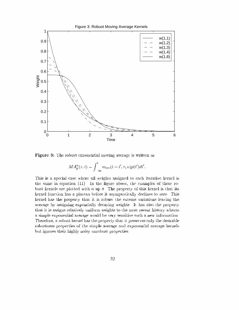
Figure 3: The robust exponential moving average is written as
MAnp (�; t) =
Z t
�1
wma(t� t0
; �; n)p(t0)dt0:
This is a special case where all weights assigned to each iterative kernel is
the same in equation (11). In the �gure above, the examples of these ro-
bust kernels are plotted with n up 8. The property of this kernel is that its
kernel function has a plateau before it asymptotically declines to zero. This
kernel has the property that it is robust the exteme variations leaving the
average by assigning expontially decaying weights. It has also the property
that it is assigns relatively uniform weights to the most recent history wheras
a simple exponential average would be very sensitive such a new information.
Therefore, a robust kernel has the property that it preserves only the desirable
robustness properties of the simple average and exponential average kernels
but ignores their highly noisy unrobust properties.
32

0 1 2 3 4 5 6−0.4
−0.2
0
0.2
0.4
0.6
0.8
1Figure 4: A Robust Differential Kernel
Time
Wei
ght
w(1,1)w(1,8)w(1,1)−w(1,8)
Figure 4: A robust di�erential kernel is presented which is based on the
di�erence between the exponential moving average with � = 1 and a robust
kernel with wma(� = 1; n = 8). By construction, the area under the kernel
sums to zero. The di�erential kernel assigns positive weights to the recent
past and negative weights to the distant past. The real-time trading model of
this paper uses a similar robust di�erential kernel in the construction of the
gearing function.
33

Table 1
Random Walk Simulations with RTT Model
USD-DEM, 1990-1996, 5 minute frequency
Description Historical p-value Percentile Mean St. Dev Skew. Kurt.
Realization (in%) [5%, 95%]
Annu. Return 9.63 0.3 -11.38, 4.03 -3.44 4.74 0.09 -0.13
Xe�ective 3.78 0.0 -20.25, -4.14 -12.11 5.09 0.13 -0.23
Re�ective 4.43 0.0 -26.42, -7.70 -16.80 5.90 0.03 -0.20
Max Drawdown 11.02 100.0 25.26, 94.86 53.79 21.36 -0.71 0.21
Deal frequency 1.68 100.0 2.20, 2.71 2.46 0.16 -0.10 -0.19
Horizon: 7 days
Xe�ective 3.47 0.0 -19.65, -4.24 -11.83 4.76 0.08 -0.15
Re�ective 1.80 0.0 -24.14, -7.21 -15.51 5.20 0.05 -0.15
Horizon: 29 days
Xe�ective 3.27 0.0 -20.21, -4.36 -12.10 4.95 0.07 -0.23
Re�ective 2.16 0.0 -27.05, -8.07 -17.45 5.91 0.02 -0.28
Horizon: 117 days
Xe�ective 4.07 0.0 -20.85, -3.42 -12.21 5.44 0.10 -0.32
Re�ective 5.10 0.0 -31.01, -6.53 -18.10 7.49 0.26 0.25
Horizon: 301 days
Xe�ective 4.62 0.0 -23.37, -2.42 -11.89 6.32 0.39 0.02
Re�ective 6.83 0.0 -27.85, -3.25 -14.56 7.49 0.35 0.16
Notes: The column under Historical Realization presents the performance of the trading model with
the actual USD-DEM series from January 1, 1990 until December 31, 1996 with 5 minute frequency.
The results under columns p-value, Percentile, Mean, St:Dev:, Skewness and Kurtosis present
the values of these statistics from 1000 replications with the random walk process. The random
walk estimation involves the regression of the actual USD-DEM returns on a constant. A simulation
sample for the random walk series with drift is obtained by sampling from the Gaussian random
number generator with the mean and the standard deviation of the residual series. The simulated
residuals are added to the conditional mean de�ned by �̂, to form a new series of returns. The new
series of the returns has the same drift in prices, the same variance and the same unconditional
distribution. From the new series of returns, the simulated price process is recovered recursively by
setting the initial price to the true price at the beginning of the sample. The trading models use the
bid and ask prices as inputs. Half of the average spread is subtracted (added) from the simulated
price process to obtain the simulated bid and ask prices.
p-values are reported in percentage terms (e.g. 8.4 refers to 8.4 percent). The de�nitions of
the performance measures for the Annu. Return, Xe�ective, Re�ective, Max Drawdown and Deal
Frequency are presented in section on Performance Measures.
34

Table 2
Random Walk Simulations with RTT Model
USD-CHF, 1990-1996, 5 minute frequency
Description Historical p-value Percentile Mean St. Dev Skew. Kurt.
Realization (in%) [5%, 95%]
Annu. Return 3.66 8.9 -12.95, 5.10 -4.15 5.61 -0.01 0.23
Xe�ective -1.68 0.7 -26.23, -6.00 -16.26 6.19 -0.02 0.03
Re�ective -4.23 0.6 -33.48, -9.80 -22.40 7.10 -0.14 -0.01
Max Drawdown 16.08 100.0 29.28, 108.66 63.68 25.19 -0.82 0.84
Deal frequency 1.29 100.0 1.82, 2.14 1.98 0.10 -0.05 -0.05
Horizon: 7 days
Xe�ective -2.96 1.2 -24.72, -6.45 -15.79 5.62 -0.04 0.18
Re�ective -4.81 0.4 -31.01, -10.55 -21.09 6.19 -0.06 0.15
Horizon: 29 days
Xe�ective -4.10 2.2 -25.72, -6.29 -16.08 5.83 -0.01 0.14
Re�ective -8.97 2.3 -34.76, -11.35 -23.61 7.05 -0.11 -0.00
Horizon: 117 days
Xe�ective -0.67 0.9 -27.49, -4.95 -16.34 6.88 -0.02 -0.13
Re�ective -1.77 0.9 -39.14, -8.91 -23.97 9.31 0.17 0.51
Horizon: 301 days
Xe�ective 1.94 0.5 -32.61, -2.87 -16.48 8.74 0.42 0.34
Re�ective 1.71 0.7 -35.24, -4.47 -18.84 9.44 0.26 0.09
Notes: The column under Historical Realization presents the performance of the trading model with
the actual USD-CHF series from January 1, 1990 until December 31, 1996 with 5 minute frequency.
The results under columns p-value, Percentile, Mean, St:Dev:, Skewness and Kurtosis present
the values of these statistics from 1000 replications with the random walk process. The random
walk estimation involves the regression of the actual USD-CHF returns on a constant. A simulation
sample for the random walk series with drift is obtained by sampling from the Gaussian random
number generator with the mean and the standard deviation of the residual series. The simulated
residuals are added to the conditional mean de�ned by �̂, to form a new series of returns. The new
series of the returns has the same drift in prices, the same variance and the same unconditional
distribution. From the new series of returns, the simulated price process is recovered recursively by
setting the initial price to the true price at the beginning of the sample. The trading models use the
bid and ask prices as inputs. Half of the average spread is subtracted (added) from the simulated
price process to obtain the simulated bid and ask prices.
p-values are reported in percentage terms (e.g. 8.4 refers to 8.4 percent). The de�nitions of
the performance measures for the Annu. Return, Xe�ective, Re�ective, Max Drawdown and Deal
Frequency are presented in section on Performance Measures.
35

Table 3
Random Walk Simulations with RTT Model
USD-FRF, 1990-1996, 5 minute frequency
Description Historical p-value Percentile Mean St. Dev Skew. Kurt.
Realization (in%) [5%, 95%]
Annu. Return 8.20 1.2 -9.92, 5.25 -2.28 4.61 0.01 0.04
X e�ective 4.80 0.2 -17.92, -2.24 -10.18 4.85 0.10 0.21
R e�ective 4.95 0.1 -23.03, -4.36 -14.13 5.63 -0.00 0.25
Max Drawdown 11.36 100.0 21.26, 83.70 47.68 19.63 -0.84 1.02
Deal frequency 1.05 100.0 1.51, 1.79 1.65 0.08 -0.13 -0.22
Horizon: 7 days
Xe�ective 3.18 0.2 -17.32, -2.56 -9.99 4.60 0.02 -0.02
Re�ective 1.97 0.2 -21.08, -5.05 -13.09 5.02 -0.00 0.01
Horizon: 29 days
Xe�ective 4.41 0.2 -17.36, -2.40 -10.15 4.64 0.02 0.08
Re�ective 3.99 0.1 -23.15, -5.68 -14.54 5.47 -0.02 0.12
Horizon: 117 days
Xe�ective 3.83 0.2 -18.87, -1.95 -10.24 5.09 0.15 0.10
Re�ective 3.77 0.1 -26.40, -4.28 -15.24 6.78 0.23 0.24
Horizon: 301 days
Xe�ective 6.35 0.2 -20.77, -0.42 -10.01 6.12 0.32 0.27
Re�ective 7.38 0.2 -25.15, -0.45 -12.37 7.43 0.21 0.20
Notes: The column under Historical Realization presents the performance of the trading model with
the actual USD-FRF series from January 1, 1990 until December 31, 1996 with 5 minute frequency.
The results under columns p-value, Percentile, Mean, St:Dev:, Skewness and Kurtosis present
the values of these statistics from 1000 replications with the random walk process. The random
walk estimation involves the regression of the actual USD-FRF returns on a constant. A simulation
sample for the random walk series with drift is obtained by sampling from the Gaussian random
number generator with the mean and the standard deviation of the residual series. The simulated
residuals are added to the conditional mean de�ned by �̂, to form a new series of returns. The new
series of the returns has the same drift in prices, the same variance and the same unconditional
distribution. From the new series of returns, the simulated price process is recovered recursively by
setting the initial price to the true price at the beginning of the sample. The trading models use the
bid and ask prices as inputs. Half of the average spread is subtracted (added) from the simulated
price process to obtain the simulated bid and ask prices.
p-values are reported in percentage terms (e.g. 8.4 refers to 8.4 percent). The de�nitions of
the performance measures for the Annu. Return, Xe�ective, Re�ective, Max Drawdown and Deal
Frequency are presented in section on Performance Measures.
36

Table 4
Random Walk Simulations with RTT Model
DEM-JPY, 1990-1996, 5 minute frequency
Description Historical p-value Percentile Mean St. Dev Skew. Kurt.
Realization (in%) [5%, 95%]
Annu. Return 6.43 2.1 -11.67, 4.66 -3.50 4.96 -0.09 -0.12
Xe�ective 3.81 0.2 -20.30, -3.17 -11.69 5.17 -0.02 0.02
Re�ective 3.45 0.1 -25.66, -6.19 -15.99 6.02 -0.12 0.19
Max Drawdown 12.03 100.0 23.12, 94.17 53.49 21.87 -0.67 0.16
Deal frequency 2.14 100.0 2.75, 3.28 3.08 0.16 0.89 0.00
Horizon: 7 days
Xe�ective 1.87 0.3 -19.66, -3.53 -11.59 4.96 -0.06 -0.14
Re�ective 0.58 0.2 -23.75, -5.93 -14.96 5.47 -0.06 -0.13
Horizon: 29 days
Xe�ective 2.12 0.3 -19.93, -3.39 -11.69 5.09 -0.02 -0.23
Re�ective 0.19 0.3 -26.45, -6.52 -16.56 6.10 -0.02 -0.23
Horizon: 117 days
Xe�ective 4.90 0.2 -20.88, -2.74 -11.79 5.48 0.01 0.11
Re�ective 5.17 0.2 -29.41, -5.42 -17.08 7.32 0.11 0.59
Horizon: 301 days
Xe�ective 5.39 0.1 -23.06, -1.93 -11.77 6.63 0.40 0.81
Re�ective 5.56 0.3 -26.64, -2.37 -13.86 7.52 0.19 0.66
Notes: The column under Historical Realization presents the performance of the trading model with
the actual DEM-JPY series from January 1, 1990 until December 31, 1996 with 5 minute frequency.
The results under columns p-value, Percentile, Mean, St:Dev:, Skewness and Kurtosis present
the values of these statistics from 1000 replications with the random walk process. The random
walk estimation involves the regression of the actual DEM-JPY returns on a constant. A simulation
sample for the random walk series with drift is obtained by sampling from the Gaussian random
number generator with the mean and the standard deviation of the residual series. The simulated
residuals are added to the conditional mean de�ned by �̂, to form a new series of returns. The new
series of the returns has the same drift in prices, the same variance and the same unconditional
distribution. From the new series of returns, the simulated price process is recovered recursively by
setting the initial price to the true price at the beginning of the sample. The trading models use the
bid and ask prices as inputs. Half of the average spread is subtracted (added) from the simulated
price process to obtain the simulated bid and ask prices.
p-values are reported in percentage terms (e.g. 8.4 refers to 8.4 percent). The de�nitions of
the performance measures for the Annu. Return, Xe�ective, Re�ective, Max Drawdown and Deal
Frequency are presented in section on Performance Measures.
37
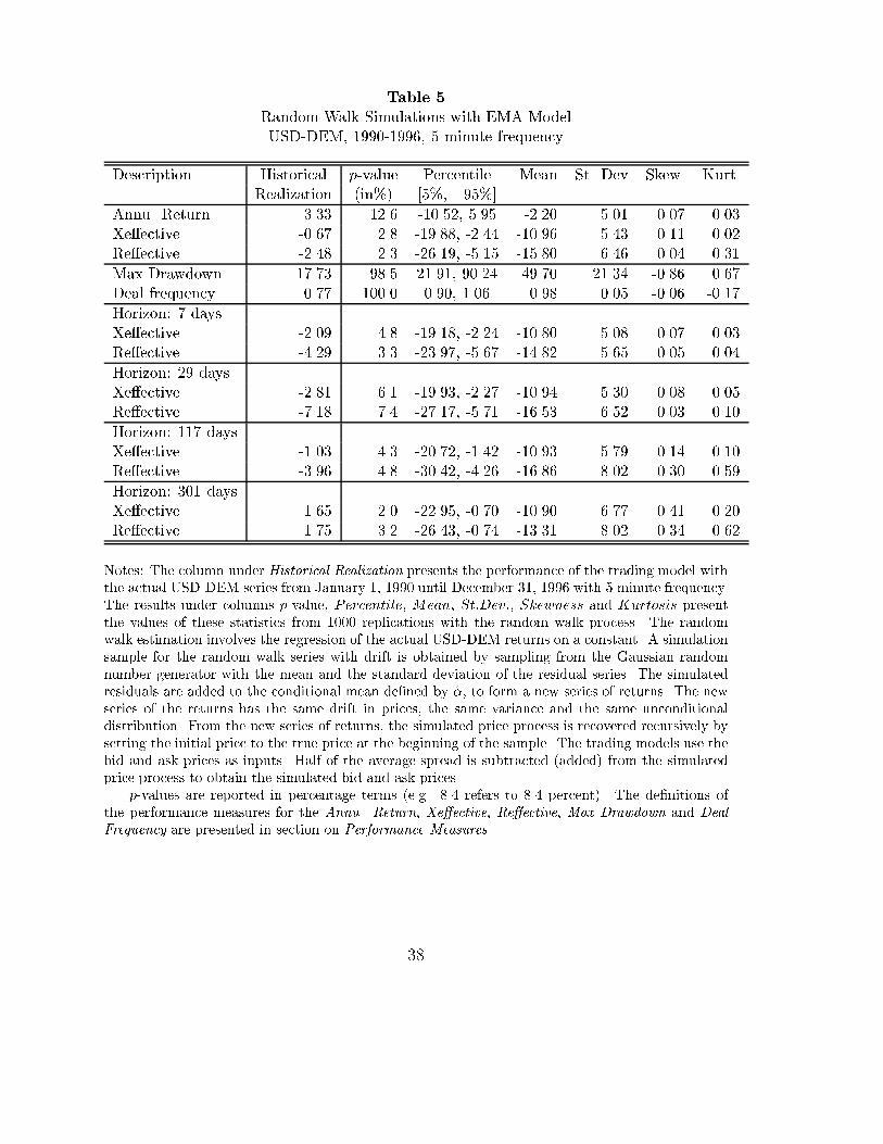
Table 5
Random Walk Simulations with EMA Model
USD-DEM, 1990-1996, 5 minute frequency
Description Historical p-value Percentile Mean St. Dev Skew. Kurt.
Realization (in%) [5%, 95%]
Annu. Return 3.33 12.6 -10.52, 5.95 -2.20 5.01 0.07 0.03
Xe�ective -0.67 2.8 -19.88, -2.44 -10.96 5.43 0.11 0.02
Re�ective -2.48 2.3 -26.19, -5.15 -15.80 6.46 0.04 0.31
Max Drawdown 17.73 98.5 21.91, 90.24 49.70 21.34 -0.86 0.67
Deal frequency 0.77 100.0 0.90, 1.06 0.98 0.05 -0.06 -0.17
Horizon: 7 days
Xe�ective -2.09 4.8 -19.18, -2.24 -10.80 5.08 0.07 0.03
Re�ective -4.29 3.3 -23.97, -5.67 -14.82 5.65 0.05 0.04
Horizon: 29 days
Xe�ective -2.81 6.1 -19.93, -2.27 -10.94 5.30 0.08 0.05
Re�ective -7.18 7.4 -27.17, -5.71 -16.53 6.52 0.03 0.10
Horizon: 117 days
Xe�ective -1.03 4.3 -20.72, -1.42 -10.93 5.79 0.14 0.10
Re�ective -3.96 4.8 -30.42, -4.26 -16.86 8.02 0.30 0.59
Horizon: 301 days
Xe�ective 1.65 2.0 -22.95, -0.70 -10.90 6.77 0.41 0.20
Re�ective 1.75 3.2 -26.43, -0.74 -13.31 8.02 0.34 0.62
Notes: The column under Historical Realization presents the performance of the trading model with
the actual USD-DEM series from January 1, 1990 until December 31, 1996 with 5 minute frequency.
The results under columns p-value, Percentile, Mean, St:Dev:, Skewness and Kurtosis present
the values of these statistics from 1000 replications with the random walk process. The random
walk estimation involves the regression of the actual USD-DEM returns on a constant. A simulation
sample for the random walk series with drift is obtained by sampling from the Gaussian random
number generator with the mean and the standard deviation of the residual series. The simulated
residuals are added to the conditional mean de�ned by �̂, to form a new series of returns. The new
series of the returns has the same drift in prices, the same variance and the same unconditional
distribution. From the new series of returns, the simulated price process is recovered recursively by
setting the initial price to the true price at the beginning of the sample. The trading models use the
bid and ask prices as inputs. Half of the average spread is subtracted (added) from the simulated
price process to obtain the simulated bid and ask prices.
p-values are reported in percentage terms (e.g. 8.4 refers to 8.4 percent). The de�nitions of
the performance measures for the Annu. Return, Xe�ective, Re�ective, Max Drawdown and Deal
Frequency are presented in section on Performance Measures.
38

Table 6
Random Walk Simulations with EMA Model
USD-CHF, 1990-1996, 5 minute frequency
Description Historical p-value Percentile Mean St. Dev Skew. Kurt.
Realization (in%) [5%, 95%]
Annu. Return 4.40 8.8 -12.87, 6.34 -3.33 5.81 0.06 -0.06
Xe�ective -0.46 0.9 -25.98, -5.64 -15.25 6.34 0.16 -0.05
Re�ective -3.00 0.4 -34.94, -10.12 -21.98 7.60 0.13 0.16
Max Drawdown 17.10 99.9 28.01, 107.44 60.72 25.19 -0.84 0.46
Deal frequency 0.85 100.0 1.10, 1.28 1.19 0.06 -0.25 0.36
Horizon: 7 days
Xe�ective -2.86 2.2 -25.07, -5.17 -15.05 5.91 0.07 -0.03
Re�ective -5.66 1.1 -32.09, -9.94 -20.99 6.65 0.05 -0.03
Horizon: 29 days
Xe�ective -3.45 2.7 -25.16, -4.88 -15.24 6.10 0.06 -0.01
Re�ective -7.26 1.8 -36.60, -11.02 -23.61 7.72 0.02 0.03
Horizon: 117 days
Xe�ective 0.39 0.7 -27.30, -4.73 -15.25 6.84 0.26 0.25
Re�ective -2.53 1.1 -40.19, -9.07 -23.34 10.02 0.64 1.23
Horizon: 301 days
Xe�ective 2.09 1.2 -29.98, -3.15 -15.15 8.47 0.63 0.89
Re�ective 2.17 1.3 -34.81, -3.86 -17.68 9.49 0.47 0.62
Notes: The column under Historical Realization presents the performance of the trading model with
the actual USD-CHF series from January 1, 1990 until December 31, 1996 with 5 minute frequency.
The results under columns p-value, Percentile, Mean, St:Dev:, Skewness and Kurtosis present
the values of these statistics from 1000 replications with the random walk process. The random
walk estimation involves the regression of the actual USD-CHF returns on a constant. A simulation
sample for the random walk series with drift is obtained by sampling from the Gaussian random
number generator with the mean and the standard deviation of the residual series. The simulated
residuals are added to the conditional mean de�ned by �̂, to form a new series of returns. The new
series of the returns has the same drift in prices, the same variance and the same unconditional
distribution. From the new series of returns, the simulated price process is recovered recursively by
setting the initial price to the true price at the beginning of the sample. The trading models use the
bid and ask prices as inputs. Half of the average spread is subtracted (added) from the simulated
price process to obtain the simulated bid and ask prices.
p-values are reported in percentage terms (e.g. 8.4 refers to 8.4 percent). The de�nitions of
the performance measures for the Annu. Return, Xe�ective, Re�ective, Max Drawdown and Deal
Frequency are presented in section on Performance Measures.
39

Table 7
Random Walk Simulations with EMA Model
USD-FRF, 1990-1996, 5 minute frequency
Description Historical p-value Percentile Mean St. Dev Skew. Kurt.
Realization (in%) [5%, 95%]
Annu. Return 6.01 6.4 -9.78, 6.35 -1.84 4.96 -0.02 -0.13
X e�ective 2.25 0.6 -19.18, -1.88 -10.31 5.36 0.06 -0.20
R e�ective 2.02 0.4 -25.20, -4.59 -14.91 6.38 -0.00 -0.02
Max Drawdown 14.52 99.6 21.44, 84.77 47.51 20.44 -0.80 0.39
Deal frequency 0.70 100.0 0.88, 1.04 0.96 0.05 -0.11 -0.14
Horizon: 7 days
Xe�ective 1.36 1.1 -18.19, -1.79 -10.19 5.03 -0.04 -0.17
Re�ective -0.07 0.4 -22.91, -4.71 -14.04 5.57 -0.05 -0.21
Horizon: 29 days
Xe�ective 1.15 1.3 -18.34, -1.93 -10.28 5.14 -0.04 -0.19
Re�ective -0.91 1.0 -25.64, -5.18 -15.64 6.28 -0.11 -0.21
Horizon: 117 days
Xe�ective 1.92 0.9 -20.03, -1.19 -10.36 5.65 0.10 -0.12
Re�ective 2.57 0.6 -29.43, -3.85 -15.92 7.75 0.28 0.24
Horizon: 301 days
Xe�ective 4.06 0.7 -22.19, 0.17 -10.18 6.75 0.38 0.04
Re�ective 5.17 0.6 -26.18, 0.27 -12.59 7.95 0.23 0.10
Notes: The column under Historical Realization presents the performance of the trading model with
the actual USD-FRF series from January 1, 1990 until December 31, 1996 with 5 minute frequency.
The results under columns p-value, Percentile, Mean, St:Dev:, Skewness and Kurtosis present
the values of these statistics from 1000 replications with the random walk process. The random
walk estimation involves the regression of the actual USD-FRF returns on a constant. A simulation
sample for the random walk series with drift is obtained by sampling from the Gaussian random
number generator with the mean and the standard deviation of the residual series. The simulated
residuals are added to the conditional mean de�ned by �̂, to form a new series of returns. The new
series of the returns has the same drift in prices, the same variance and the same unconditional
distribution. From the new series of returns, the simulated price process is recovered recursively by
setting the initial price to the true price at the beginning of the sample. The trading models use the
bid and ask prices as inputs. Half of the average spread is subtracted (added) from the simulated
price process to obtain the simulated bid and ask prices.
p-values are reported in percentage terms (e.g. 8.4 refers to 8.4 percent). The de�nitions of
the performance measures for the Annu. Return, Xe�ective, Re�ective, Max Drawdown and Deal
Frequency are presented in section on Performance Measures.
40

Table 8
Random Walk Simulations with EMA Model
DEM-JPY, 1990-1996, 5 minute frequency
Description Historical p-value Percentile Mean St. Dev Skew. Kurt.
Realization (in%) [5%, 95%]
Annu. Return 7.09 6.6 -8.71, 7.56 -0.75 5.06 -0.07 -0.02
Xe�ective 2.63 1.4 -18.35, -0.74 -9.24 5.33 0.15 0.23
Re�ective 2.97 1.0 -24.36, -2.42 -13.54 6.65 0.07 0.49
Max Drawdown 13.06 99.6 20.45, 79.17 44.28 18.91 -0.95 1.03
Deal frequency 0.75 99.9 0.82, 1.08 0.95 0.08 -0.12 -0.95
Horizon: 7 days
Xe�ective 1.81 2.0 -17.04, -0.89 -8.90 5.04 0.07 0.11
Re�ective 0.57 1.3 -21.54, -3.70 -12.56 5.63 0.11 0.24
Horizon: 29 days
Xe�ective 1.94 1.6 -17.60, -0.56 -9.16 5.17 0.08 0.09
Re�ective 1.47 0.6 -25.08, -3.61 -14.27 6.43 0.14 0.20
Horizon: 117 days
Xe�ective 3.43 0.9 -19.19, -0.18 -9.24 5.87 0.27 0.44
Re�ective 4.26 0.9 -29.00, -2.07 -14.60 8.45 0.53 1.49
Horizon: 301 days
Xe�ective 3.76 1.1 -22.51, 1.29 -9.60 7.18 0.48 0.88
Re�ective 4.31 1.0 -24.87, 2.29 -11.29 8.42 0.22 0.71
Notes: The column under Historical Realization presents the performance of the trading model with
the actual DEM-JPY series from January 1, 1990 until December 31, 1996 with 5 minute frequency.
The results under columns p-value, Percentile, Mean, St:Dev:, Skewness and Kurtosis present
the values of these statistics from 1000 replications with the random walk process. The random
walk estimation involves the regression of the actual DEM-JPY returns on a constant. A simulation
sample for the random walk series with drift is obtained by sampling from the Gaussian random
number generator with the mean and the standard deviation of the residual series. The simulated
residuals are added to the conditional mean de�ned by �̂, to form a new series of returns. The new
series of the returns has the same drift in prices, the same variance and the same unconditional
distribution. From the new series of returns, the simulated price process is recovered recursively by
setting the initial price to the true price at the beginning of the sample. The trading models use the
bid and ask prices as inputs. Half of the average spread is subtracted (added) from the simulated
price process to obtain the simulated bid and ask prices.
p-values are reported in percentage terms (e.g. 8.4 refers to 8.4 percent). The de�nitions of
the performance measures for the Annu. Return, Xe�ective, Re�ective, Max Drawdown and Deal
Frequency are presented in section on Performance Measures.
41

Table 9
GARCH(1,1) Parameter Estimates, 1990-1996, 5 minute frequency
USD-DEM USD-CHF USD-FRF DEM-JPY
�0 4:95 (4:23) 0:11 (0:12) 9:38 (7:09) 2:97 (4:03)
�1 0.1111 (0.0005) 0.1032 (0.0007) 0.1572 (0.0007) 0.0910 (0.0005)
�1 0.8622 (0.0007) 0.8578 (0.0009) 0.8137 (0.0009) 0.8988 (0.0006)
LL 6.45 6.17 6.29 6.34
Q(12) 5.08 32.96 4.04 55.94
�̂�2 1.04 1.03 1.07 1.05
�̂sk -0.07 -0.03 -0.05 0.16
�̂ku 11.73 7.28 22.93 27.73
Notes: �0 values are 10�9. The numbers in paratheses are the standard errors. The standard errors
of �0 are 10�11. LL is the average log likelihood value. Q(12) is the Ljung and Box portmanteu test
for serial correlation and distributed �2 with 12 degrees of freedom. The �2
0:05(12) is 21.03. �̂
�
2 , �̂sk
and �̂ku
are the variance, skewness and the excess kurtosis of the residuals.
42

Table 10
GARCH(1,1) Simulations with RTT Model
USD-DEM, 1990-1996, 5 minute frequency
Description Historical p-value Percentile Mean St. Dev Skew. Kurt.
Realization (in%) [5%, 95%]
Annu. Return 9.63 0.4 -11.14, 5.12 -3.27 4.90 -0.08 -0.01
X e�ective 3.78 0.1 -20.40, -3.16 -11.88 5.18 -0.07 -0.11
R e�ective 4.43 0.0 -26.60, -6.37 -16.50 6.10 -0.14 -0.05
Max Drawdown 11.02 100.0 24.17, 93.96 53.33 21.50 -0.73 0.30
Deal frequency 1.68 100.0 2.14, 2.64 2.39 0.15 -0.02 -0.15
Horizon: 7 days
Xe�ective 3.47 0.2 -19.56, -3.49 -11.64 4.90 -0.06 -0.03
Re�ective 1.80 0.0 -24.19, -6.58 -15.37 5.38 -0.08 -0.05
Horizon: 29 days
Xe�ective 3.27 0.2 -19.95, -3.29 -11.86 5.00 -0.12 -0.04
Re�ective 2.16 0.1 -26.92, -6.75 -17.20 6.04 -0.20 -0.03
Horizon: 117 days
Xe�ective 4.07 0.1 -21.24, -2.77 -11.91 5.56 0.03 -0.28
Re�ective 5.10 0.1 -30.17, -5.44 -17.57 7.60 0.29 0.31
Horizon: 301 days
Xe�ective 4.62 0.2 -22.73, -1.48 -11.73 6.42 0.28 0.16
Re�ective 6.83 0.3 -27.64, -2.01 -14.28 7.72 0.26 0.38
Notes: The column under Historical Realization presents the performance of the trading model with
the actual USD-DEM series from January 1, 1990 until December 31, 1996 with 5 minute frequency.
The results under columns p-value, Percentile, Mean, St:Dev:, Skewness and Kurtosis present
the values of these statistics from 1000 replications with the random walk process. The parameters
and the normalized residuals are estimated from the foreign exchange returns using the maximum
likelihood procedure. The simulated returns for the GARCH(1,1) process are generated from the
simulated residuals and the estimated parameters. From the new series of returns, the simulated
price process is recovered recursively by setting the initial price to the true price at the beginning
of the sample. The trading models use the bid and ask prices as inputs. Half of the average spread
is subtracted (added) from the simulated price process to obtain the simulated bid and ask prices.
p-values are reported in percentage terms (e.g. 8.4 refers to 8.4 percent). The de�nitions of
the performance measures for the Annu. Return, Xe�ective, Re�ective, Max Drawdown and Deal
Frequency are presented in section on Performance Measures.
43
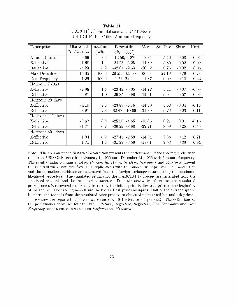
Table 11
GARCH(1,1) Simulations with RTT Model
USD-CHF, 1990-1996, 5 minute frequency
Description Historical p-value Percentile Mean St. Dev Skew. Kurt.
Realization (in%) [5%, 95%]
Annu. Return 3.66 8.4 -12.56, 4.87 -3.84 5.46 -0.08 -0.04
Xe�ective -1.68 1.4 -24.23, -5.25 -14.89 5.80 -0.02 -0.09
Re�ective -4.23 0.9 -32.01, -9.33 -20.59 6.73 -0.02 0.05
Max Drawdown 16.08 100.0 28.25, 105.09 60.58 24.16 -0.76 0.28
Deal frequency 1.29 100.0 1.72, 2.02 1.87 0.09 -0.12 0.22
Horizon: 7 days
Xe�ective -2.96 1.6 -23.49, -6.05 -14.72 5.44 -0.07 -0.08
Re�ective -4.81 1.0 -29.35, -9.96 -19.61 6.01 -0.07 -0.06
Horizon: 29 days
Xe�ective -4.10 2.6 -23.87, -5.76 -14.90 5.58 -0.04 -0.13
Re�ective -8.97 2.8 -32.67, -10.69 -21.80 6.76 -0.03 -0.11
Horizon: 117 days
Xe�ective -0.67 0.8 -25.50, -4.55 -15.06 6.27 0.01 -0.15
Re�ective -1.77 0.7 -36.29, -8.68 -22.21 8.69 0.25 0.45
Horizon: 301 days
Xe�ective 1.94 0.9 -27.44, -2.59 -14.54 7.68 0.42 0.71
Re�ective 1.71 1.5 -31.28, -3.58 -17.01 8.58 0.30 0.94
Notes: The column under Historical Realization presents the performance of the trading model with
the actual USD-CHF series from January 1, 1990 until December 31, 1996 with 5 minute frequency.
The results under columns p-value, Percentile, Mean, St:Dev:, Skewness and Kurtosis present
the values of these statistics from 1000 replications with the random walk process. The parameters
and the normalized residuals are estimated from the foreign exchange returns using the maximum
likelihood procedure. The simulated returns for the GARCH(1,1) process are generated from the
simulated residuals and the estimated parameters. From the new series of returns, the simulated
price process is recovered recursively by setting the initial price to the true price at the beginning
of the sample. The trading models use the bid and ask prices as inputs. Half of the average spread
is subtracted (added) from the simulated price process to obtain the simulated bid and ask prices.
p-values are reported in percentage terms (e.g. 8.4 refers to 8.4 percent). The de�nitions of
the performance measures for the Annu. Return, Xe�ective, Re�ective, Max Drawdown and Deal
Frequency are presented in section on Performance Measures.
44

Table 12
GARCH(1,1) Simulations with RTT Model
USD-FRF, 1990-1996, 5 minute frequency
Description Historical p-value Percentile Mean St. Dev Skew. Kurt.
Realization (in%) [5%, 95%]
Annu. Return 8.20 0.9 -9.21, 5.50 -2.01 4.44 -0.11 -0.10
X e�ective 4.80 0.1 -17.54, -2.17 -9.84 4.67 -0.03 -0.03
R e�ective 4.95 0.1 -22.39, -4.17 -13.71 5.54 -0.09 0.22
Max Drawdown 11.36 99.9 21.85, 78.99 46.00 18.13 -0.82 0.99
Deal frequency 1.05 100.0 1.46, 1.72 1.59 0.08 -1.05 8.78
Horizon: 7 days
Xe�ective 3.18 0.3 -16.67, -2.28 -9.73 4.42 -0.06 -0.00
Re�ective 1.97 0.1 -20.62, -4.78 -12.88 4.86 -0.03 0.11
Horizon: 29 days
Xe�ective 4.41 0.1 -17.02, -2.44 -9.84 4.49 -0.08 -0.12
Re�ective 3.99 0.0 -22.63, -5.14 -14.19 5.44 -0.00 0.57
Horizon: 117 days
Xe�ective 3.83 0.4 -18.01, -1.68 -9.87 4.95 -0.00 0.14
Re�ective 3.77 0.2 -26.15, -4.02 -14.77 6.77 0.21 1.07
Horizon: 301 days
Xe�ective 6.35 0.1 -20.12, -0.58 -9.72 5.87 0.33 0.35
Re�ective 7.38 0.2 -24.06, -1.06 -12.00 7.06 0.33 0.85
Notes: The column under Historical Realization presents the performance of the trading model with
the actual USD-FRF series from January 1, 1990 until December 31, 1996 with 5 minute frequency.
The results under columns p-value, Percentile, Mean, St:Dev:, Skewness and Kurtosis present
the values of these statistics from 1000 replications with the random walk process. The parameters
and the normalized residuals are estimated from the foreign exchange returns using the maximum
likelihood procedure. The simulated returns for the GARCH(1,1) process are generated from the
simulated residuals and the estimated parameters. From the new series of returns, the simulated
price process is recovered recursively by setting the initial price to the true price at the beginning
of the sample. The trading models use the bid and ask prices as inputs. Half of the average spread
is subtracted (added) from the simulated price process to obtain the simulated bid and ask prices.
p-values are reported in percentage terms (e.g. 8.4 refers to 8.4 percent). The de�nitions of
the performance measures for the Annu. Return, Xe�ective, Re�ective, Max Drawdown and Deal
Frequency are presented in section on Performance Measures.
45

Table 13
GARCH(1,1) Simulations with RTT Model
DEM-JPY, 1990-1996, 5 minute frequency
Description Historical p-value Percentile Mean St. Dev Skew. Kurt.
Realization (in%) [5%, 95%]
Annu. Return 6.43 1.2 -10.75, 3.59 -3.51 4.36 -0.12 0.03
Xe�ective 3.81 0.4 -17.00, -2.75 -9.86 4.48 -0.12 0.11
Re�ective 3.45 0.4 -21.74, -4.82 -13.35 5.21 -0.19 0.35
Max Drawdown 12.03 100.0 22.13, 86.56 48.77 19.70 -0.71 0.26
Deal frequency 2.14 100.0 2.53, 2.78 2.66 0.08 -1.39 15.91
Horizon: 7 days
Xe�ective 1.87 0.6 -17.11, -3.02 -9.90 4.34 -0.12 0.08
Re�ective 0.58 0.6 -20.50, -4.92 -12.57 4.83 -0.07 0.22
Horizon: 29 days
Xe�ective 2.12 0.5 -17.31, -2.76 -9.95 4.43 -0.10 -0.03
Re�ective 0.19 0.7 -22.38, -5.08 -13.75 5.29 -0.08 0.01
Horizon: 117 days
Xe�ective 4.90 0.2 -17.74, -2.10 -9.90 4.67 -0.12 0.05
Re�ective 5.17 0.2 -24.77, -3.69 -14.33 6.25 0.04 0.36
Horizon: 301 days
Xe�ective 5.39 0.4 -19.13, -1.74 -9.76 5.35 0.29 0.68
Re�ective 5.56 0.5 -23.34, -2.57 -12.08 6.47 0.34 1.07
Notes: The column under Historical Realization presents the performance of the trading model with
the actual DEM-JPY series from January 1, 1990 until December 31, 1996 with 5 minute frequency.
The results under columns p-value, Percentile, Mean, St:Dev:, Skewness and Kurtosis present
the values of these statistics from 1000 replications with the random walk process. The parameters
and the normalized residuals are estimated from the foreign exchange returns using the maximum
likelihood procedure. The simulated returns for the GARCH(1,1) process are generated from the
simulated residuals and the estimated parameters. From the new series of returns, the simulated
price process is recovered recursively by setting the initial price to the true price at the beginning
of the sample. The trading models use the bid and ask prices as inputs. Half of the average spread
is subtracted (added) from the simulated price process to obtain the simulated bid and ask prices.
p-values are reported in percentage terms (e.g. 8.4 refers to 8.4 percent). The de�nitions of
the performance measures for the Annu. Return, Xe�ective, Re�ective, Max Drawdown and Deal
Frequency are presented in section on Performance Measures.
46

Table 14
GARCH(1,1) Simulations with EMA Model
USD-DEM, 1990-1996, 5 minute frequency
Description Historical p-value Percentile Mean St. Dev Skew. Kurt.
Realization (in%) [5%, 95%]
Annu. Return 3.33 14.1 -9.83, 5.97 -1.98 4.88 0.01 -0.07
Xe�ective -0.67 2.3 -19.63, -2.05 -10.76 5.30 0.12 -0.07
Re�ective -2.48 1.8 -26.07, -5.04 -15.69 6.38 0.05 0.01
Max Drawdown 17.73 99.2 22.60, 85.88 48.61 19.71 -0.86 0.71
Deal frequency 0.77 100.0 0.88, 1.05 0.96 0.05 -0.06 0.00
Horizon: 7 days
Xe�ective -2.09 3.8 -18.40, -2.60 -10.59 4.96 0.03 -0.05
Re�ective -4.29 2.8 -23.51, -5.50 -14.63 5.56 0.03 -0.05
Horizon: 29 days
Xe�ective -2.81 5.8 -19.20, -2.60 -10.75 5.16 0.12 -0.04
Re�ective -7.18 7.2 -27.32, -6.14 -16.46 6.46 0.16 0.09
Horizon: 117 days
Xe�ective -1.03 3.1 -20.42, -1.90 -10.77 5.69 0.20 -0.00
Re�ective -3.96 3.8 -31.27, -4.67 -16.88 8.16 0.45 0.73
Horizon: 301 days
Xe�ective 1.65 2.1 -22.35, -0.52 -10.73 6.68 0.48 0.43
Re�ective 1.75 2.4 -26.80, -1.28 -13.28 7.69 0.23 -0.09
Notes: The column under Historical Realization presents the performance of the trading model with
the actual USD-DEM series from January 1, 1990 until December 31, 1996 with 5 minute frequency.
The results under columns p-value, Percentile, Mean, St:Dev:, Skewness and Kurtosis present
the values of these statistics from 1000 replications with the random walk process. The parameters
and the normalized residuals are estimated from the foreign exchange returns using the maximum
likelihood procedure. The simulated returns for the GARCH(1,1) process are generated from the
simulated residuals and the estimated parameters. From the new series of returns, the simulated
price process is recovered recursively by setting the initial price to the true price at the beginning
of the sample. The trading models use the bid and ask prices as inputs. Half of the average spread
is subtracted (added) from the simulated price process to obtain the simulated bid and ask prices.
p-values are reported in percentage terms (e.g. 8.4 refers to 8.4 percent). The de�nitions of
the performance measures for the Annu. Return, Xe�ective, Re�ective, Max Drawdown and Deal
Frequency are presented in section on Performance Measures.
47

Table 15
GARCH(1,1) Simulations with EMA Model
USD-CHF, 1990-1996, 5 minute frequency
Description Historical p-value Percentile Mean St. Dev Skew. Kurt.
Realization (in%) [5%, 95%]
Annu. Return 4.40 9.6 -12.86, 6.13 -3.16 5.80 0.03 -0.23
X e�ective -0.46 0.7 -26.27, -4.95 -15.13 6.35 0.12 -0.18
R e�ective -3.00 0.5 -34.67, -9.17 -21.92 7.59 0.06 0.13
Max Drawdown 17.10 99.9 27.98, 109.09 60.09 24.80 -0.80 0.18
Deal frequency 0.85 100.0 1.08, 1.28 1.18 0.06 -0.10 0.38
Horizon: 7 days
Xe�ective -2.86 1.7 -24.57, -5.53 -14.87 5.92 0.04 -0.22
Re�ective -5.66 1.2 -31.76, -10.13 -20.83 6.71 0.03 -0.25
Horizon: 29 days
Xe�ective -3.45 2.7 -25.46, -5.05 -15.09 6.15 0.01 -0.32
Re�ective -7.26 1.5 -37.07, -9.83 -23.56 7.93 -0.05 -0.23
Horizon: 117 days
Xe�ective 0.39 0.7 -26.72, -3.87 -15.18 6.88 0.18 0.00
Re�ective -2.53 1.5 -39.88, -7.71 -23.42 9.98 0.41 0.65
Horizon: 301 days
Xe�ective 2.09 1.3 -30.15, -2.48 -14.94 8.45 0.55 0.63
Re�ective 2.17 1.5 -34.44, -2.83 -17.51 9.43 0.43 0.64
Notes: The column under Historical Realization presents the performance of the trading model with
the actual USD-CHF series from January 1, 1990 until December 31, 1996 with 5 minute frequency.
The results under columns p-value, Percentile, Mean, St:Dev:, Skewness and Kurtosis present
the values of these statistics from 1000 replications with the random walk process. The parameters
and the normalized residuals are estimated from the foreign exchange returns using the maximum
likelihood procedure. The simulated returns for the GARCH(1,1) process are generated from the
simulated residuals and the estimated parameters. From the new series of returns, the simulated
price process is recovered recursively by setting the initial price to the true price at the beginning
of the sample. The trading models use the bid and ask prices as inputs. Half of the average spread
is subtracted (added) from the simulated price process to obtain the simulated bid and ask prices.
p-values are reported in percentage terms (e.g. 8.4 refers to 8.4 percent). The de�nitions of
the performance measures for the Annu. Return, Xe�ective, Re�ective, Max Drawdown and Deal
Frequency are presented in section on Performance Measures.
48

Table 16
GARCH(1,1) Simulations with EMA Model
USD-FRF, 1990-1996, 5 minute frequency
Description Historical p-value Percentile Mean St. Dev Skew. Kurt.
Realization (in%) [5%, 95%]
Annu. Return 6.01 4.6 -8.91, 5.88 -1.60 4.61 -0.12 -0.03
Xe�ective 2.25 0.6 -18.14, -1.83 -10.03 5.01 -0.04 -0.18
Re�ective 2.02 0.4 -25.25, -4.27 -14.69 6.19 -0.02 0.03
Max Drawdown 14.52 99.7 20.79, 80.38 46.04 18.73 -0.77 0.51
Deal frequency 0.70 100.0 0.85, 1.02 0.93 0.05 -1.44 13.00
Horizon: 7 days
Xe�ective 1.36 0.8 -17.54, -2.43 -9.91 4.70 -0.06 -0.04
Re�ective -0.07 0.6 -22.08, -5.40 -13.76 5.28 -0.03 -0.01
Horizon: 29 days
Xe�ective 1.15 0.9 -18.06, -1.97 -9.98 4.87 -0.03 -0.07
Re�ective -0.91 0.9 -25.40, -5.43 -15.27 6.18 -0.02 -0.00
Horizon: 117 days
Xe�ective 1.92 0.7 -18.90, -1.22 -10.08 5.34 0.07 -0.22
Re�ective 2.57 0.5 -29.72, -3.32 -15.78 8.00 0.49 0.78
Horizon: 301 days
Xe�ective 4.06 0.8 -20.53, 0.42 -9.87 6.39 0.35 0.50
Re�ective 5.17 0.7 -26.23, 0.42 -12.35 7.91 0.27 0.31
Notes: The column under Historical Realization presents the performance of the trading model with
the actual USD-FRF series from January 1, 1990 until December 31, 1996 with 5 minute frequency.
The results under columns p-value, Percentile, Mean, St:Dev:, Skewness and Kurtosis present
the values of these statistics from 1000 replications with the random walk process. The parameters
and the normalized residuals are estimated from the foreign exchange returns using the maximum
likelihood procedure. The simulated returns for the GARCH(1,1) process are generated from the
simulated residuals and the estimated parameters. From the new series of returns, the simulated
price process is recovered recursively by setting the initial price to the true price at the beginning
of the sample. The trading models use the bid and ask prices as inputs. Half of the average spread
is subtracted (added) from the simulated price process to obtain the simulated bid and ask prices.
p-values are reported in percentage terms (e.g. 8.4 refers to 8.4 percent). The de�nitions of
the performance measures for the Annu. Return, Xe�ective, Re�ective, Max Drawdown and Deal
Frequency are presented in section on Performance Measures.
49

Table 17
GARCH(1,1) Simulations with EMA Model
DEM-JPY, 1990-1996, 5 minute frequency
Description Historical p-value Percentile Mean St. Dev Skew. Kurt.
Realization (in%) [5%, 95%]
Annu. Return 7.09 2.8 -8.77, 5.80 -1.59 4.38 -0.11 -0.19
Xe�ective 2.63 0.5 -16.67, -0.91 -8.72 4.73 0.02 -0.27
Re�ective 2.97 0.2 -22.03, -3.34 -12.73 5.78 0.02 -0.15
Max Drawdown 13.06 99.8 19.69, 75.94 43.01 17.61 -0.79 0.31
Deal frequency 0.75 97.8 0.77, 0.93 0.84 0.05 -1.85 19.57
Horizon: 7 days
Xe�ective 1.81 1.2 -16.00, -1.11 -8.65 4.50 -0.05 -0.15
Re�ective 0.57 0.6 -19.98, -3.38 -11.94 5.10 0.01 0.01
Horizon: 29 days
Xe�ective 1.94 0.6 -16.32, -1.22 -8.76 4.59 0.01 -0.20
Re�ective 1.47 0.3 -22.86, -4.23 -13.26 5.73 0.12 0.09
Horizon: 117 days
Xe�ective 3.43 0.4 -17.14, -0.35 -8.68 5.04 0.07 -0.26
Re�ective 4.26 0.3 -25.94, -2.47 -13.56 7.20 0.32 0.29
Horizon: 301 days
Xe�ective 0.76 3.6 -19.12, 0.14 -8.73 5.87 0.34 0.10
Re�ective 2.31 2.4 -22.65, 0.30 -11.09 7.22 0.35 0.51
Notes: The column under Historical Realization presents the performance of the trading model with
the actual DEM-JPY series from January 1, 1990 until December 31, 1996 with 5 minute frequency.
The results under columns p-value, Percentile, Mean, St:Dev:, Skewness and Kurtosis present
the values of these statistics from 1000 replications with the random walk process. The parameters
and the normalized residuals are estimated from the foreign exchange returns using the maximum
likelihood procedure. The simulated returns for the GARCH(1,1) process are generated from the
simulated residuals and the estimated parameters. From the new series of returns, the simulated
price process is recovered recursively by setting the initial price to the true price at the beginning
of the sample. The trading models use the bid and ask prices as inputs. Half of the average spread
is subtracted (added) from the simulated price process to obtain the simulated bid and ask prices.
p-values are reported in percentage terms (e.g. 8.4 refers to 8.4 percent). The de�nitions of
the performance measures for the Annu. Return, Xe�ective, Re�ective, Max Drawdown and Deal
Frequency are presented in section on Performance Measures.
50

Table 18
AR(4)-GARCH(1,1) Parameter Estimates, 1990-1996, 5 minute frequency
USD-DEM USD-CHF USD-FRF DEM-JPY
�0 3.90 (3.40) 8.19 (9.03) 7.28 (5.80) 2.92 (3.93)
�1 0.099 (0.0005) 0.0874 (0.0006) 0.1349 (0.0007) 0.088 (0.0005)
�1 0.8796 (0.0006) 0.8833 (0.0007) 0.8411 (0.0008) 0.9008 (0.0006)
1 -0.176 (0.001) -0.208 (0.001) -0.200 (0.002) -0.130 (0.002)
2 -0.011 (0.001) -0.031 (0.002) -0.025 (0.002) -0.090 (0.002)
3 0.003 (0.001) -0.001 (0.002) -0.005 (0.002) -0.005 (0.002)
4 -0.004(0.001) -0.002 (0.001) -0.008 (0.002) -0.010 (0.002)�LL 6.46 6.19 6.30 6.35
Q(12) 0.21 0.69 0.10 0.81
�̂�2 1.04 1.03 1.07 1.05
�̂sk -0.07 -0.04 -0.05 0.15
�̂ku 12.29 7.86 21.84 27.98
Notes: �0 values are 10�9. The numbers in paratheses are the standard errors. The standard errors
of �0 are 10�11. LL is the average log likelihood value. Q(12) refer to the Ljung-Box portmanteu
test for serial correlation and it is distributed �2 with 12 degrees of freedom. The �2
0:05(12) is 21.03.
�̂�
2 , �̂sk
and �̂ku
are the variance, skewness and the excess kurtosis of the residuals.
51

Table 19
AR(4)-GARCH(1,1) Simulations with RTT Model
USD-DEM, 1990-1996, 5 minute frequency
Description Historical p-value Percentile Mean St. Dev Skew. Kurt.
Realization (in%) [5%, 95%]
Annu. Return 9.63 0.1 -10.46, 3.13 -3.68 4.13 -0.01 -0.16
X e�ective 3.78 0.1 -16.72, -3.16 -9.95 4.27 -0.02 -0.18
R e�ective 4.43 0.0 -21.37, -5.28 -13.37 4.93 -0.07 -0.15
Max Drawdown 11.02 100.0 21.73, 84.55 49.07 19.16 -0.59 0.03
Deal frequency 1.68 100.0 1.89, 2.35 2.12 0.14 -0.04 -0.26
Horizon: 7 days
Xe�ective 3.47 0.1 -16.53, -2.86 -9.72 4.13 0.01 -0.18
Re�ective 1.80 0.2 -19.63, -4.95 -12.33 4.45 -0.01 -0.17
Horizon: 29 days
Xe�ective 3.27 0.1 -16.90, -3.24 -9.94 4.21 0.00 -0.11
Re�ective 2.16 0.1 -21.54, -5.87 -13.67 4.87 -0.02 -0.02
Horizon: 117 days
Xe�ective 4.07 0.1 -17.37, -2.83 -9.97 4.50 0.00 -0.26
Re�ective 5.10 0.0 -24.10, -4.75 -14.17 5.98 0.23 0.21
Horizon: 301 days
Xe�ective 4.62 0.1 -18.19, -2.01 -9.83 4.95 0.19 0.16
Re�ective 6.83 0.1 -22.90, -2.91 -12.15 6.15 0.34 0.53
Notes: The column under Historical Realization presents the performance of the trading model with
the actual USD-DEM series from January 1, 1990 until December 31, 1996 with 5 minute frequency.
The results under columns p-value, Percentile, Mean, St:Dev:, Skewness and Kurtosis present
the values of these statistics from 1000 replications with the random walk process. The parameters
and the normalized residuals are estimated from the foreign exchange returns using the maximum
likelihood procedure. The simulated returns for the AR(4)-GARCH(1,1) process are generated from
the simulated residuals and the estimated parameters. From the new series of returns, the simulated
price process is recovered recursively by setting the initial price to the true price at the beginning
of the sample. The trading models use the bid and ask prices as inputs. Half of the average spread
is subtracted (added) from the simulated price process to obtain the simulated bid and ask prices.
p-values are reported in percentage terms (e.g. 8.4 refers to 8.4 percent). The de�nitions of
the performance measures for the Annu. Return, Xe�ective, Re�ective, Max Drawdown and Deal
Frequency are presented in section on Performance Measures.
52

Table 20
AR(4)-GARCH(1,1) Simulations with RTT Model
USD-CHF, 1990-1996, 5 minute frequency
Description Historical p-value Percentile Mean St. Dev Skew. Kurt.
Realization (in%) [5%, 95%]
Annu. Return 3.66 3.7 -11.57, 3.36 -4.06 4.54 -0.06 -0.05
Xe�ective -1.68 1.9 -19.54, -3.94 -11.72 4.77 -0.06 -0.06
Re�ective -4.23 2.3 -24.29, -6.48 -15.75 5.50 -0.10 0.20
Max Drawdown 16.08 99.7 24.11, 93.75 53.88 21.64 -0.62 0.03
Deal frequency 1.29 99.9 1.40, 1.65 1.52 0.08 -0.02 0.04
Horizon: 7 days
Xe�ective -2.96 2.8 -19.15, -4.22 -11.47 4.53 -0.05 -0.02
Re�ective -4.81 2.4 -23.05, -6.74 -14.63 4.92 -0.05 0.01
Horizon: 29 days
Xe�ective -4.10 4.6 -19.36, -4.23 -11.66 4.59 -0.04 -0.02
Re�ective -8.97 9.7 -25.17, -7.02 -16.06 5.39 -0.07 0.02
Horizon: 117 days
Xe�ective -0.67 1.3 -19.93, -3.51 -11.81 5.00 -0.07 -0.07
Re�ective -1.77 1.4 -27.35, -6.41 -16.98 6.57 0.09 0.42
Horizon: 301 days
Xe�ective 1.94 0.8 -21.30, -2.21 -11.51 6.08 0.30 0.44
Re�ective 1.71 1.1 -25.53, -2.90 -13.95 7.27 0.46 1.59
Notes: The column under Historical Realization presents the performance of the trading model with
the actual USD-CHF series from January 1, 1990 until December 31, 1996 with 5 minute frequency.
The results under columns p-value, Percentile, Mean, St:Dev:, Skewness and Kurtosis present
the values of these statistics from 1000 replications with the random walk process. The parameters
and the normalized residuals are estimated from the foreign exchange returns using the maximum
likelihood procedure. The simulated returns for the AR(4)-GARCH(1,1) process are generated from
the simulated residuals and the estimated parameters. From the new series of returns, the simulated
price process is recovered recursively by setting the initial price to the true price at the beginning
of the sample. The trading models use the bid and ask prices as inputs. Half of the average spread
is subtracted (added) from the simulated price process to obtain the simulated bid and ask prices.
p-values are reported in percentage terms (e.g. 8.4 refers to 8.4 percent). The de�nitions of
the performance measures for the Annu. Return, Xe�ective, Re�ective, Max Drawdown and Deal
Frequency are presented in section on Performance Measures.
53
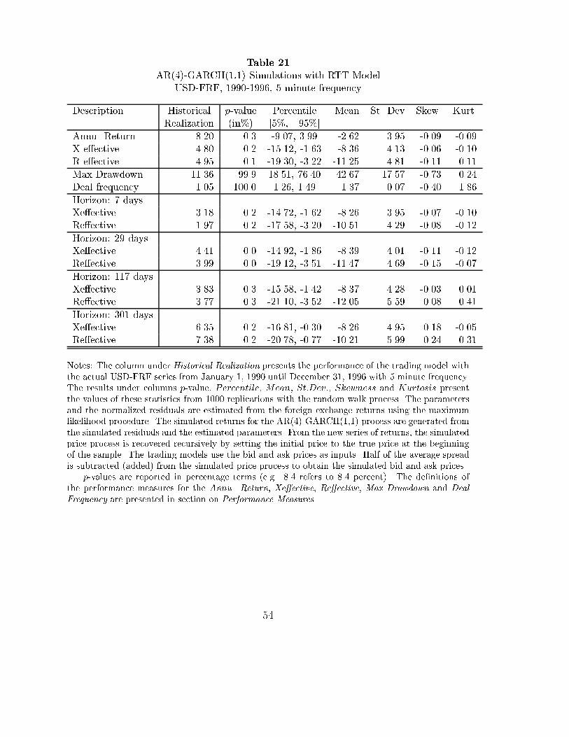
Table 21
AR(4)-GARCH(1,1) Simulations with RTT Model
USD-FRF, 1990-1996, 5 minute frequency
Description Historical p-value Percentile Mean St. Dev Skew. Kurt.
Realization (in%) [5%, 95%]
Annu. Return 8.20 0.3 -9.07, 3.99 -2.62 3.95 -0.09 -0.09
X e�ective 4.80 0.2 -15.12, -1.63 -8.36 4.13 -0.06 -0.10
R e�ective 4.95 0.1 -19.30, -3.22 -11.25 4.81 -0.11 0.11
Max Drawdown 11.36 99.9 18.51, 76.40 42.67 17.57 -0.73 0.24
Deal frequency 1.05 100.0 1.26, 1.49 1.37 0.07 -0.40 1.86
Horizon: 7 days
Xe�ective 3.18 0.2 -14.72, -1.62 -8.26 3.95 -0.07 -0.10
Re�ective 1.97 0.2 -17.58, -3.20 -10.51 4.29 -0.08 -0.12
Horizon: 29 days
Xe�ective 4.41 0.0 -14.92, -1.86 -8.39 4.01 -0.11 -0.12
Re�ective 3.99 0.0 -19.12, -3.51 -11.47 4.69 -0.15 -0.07
Horizon: 117 days
Xe�ective 3.83 0.3 -15.58, -1.42 -8.37 4.28 -0.03 0.01
Re�ective 3.77 0.3 -21.10, -3.52 -12.05 5.59 0.08 0.41
Horizon: 301 days
Xe�ective 6.35 0.2 -16.81, -0.30 -8.26 4.95 0.18 -0.05
Re�ective 7.38 0.2 -20.78, -0.77 -10.21 5.99 0.24 0.31
Notes: The column under Historical Realization presents the performance of the trading model with
the actual USD-FRF series from January 1, 1990 until December 31, 1996 with 5 minute frequency.
The results under columns p-value, Percentile, Mean, St:Dev:, Skewness and Kurtosis present
the values of these statistics from 1000 replications with the random walk process. The parameters
and the normalized residuals are estimated from the foreign exchange returns using the maximum
likelihood procedure. The simulated returns for the AR(4)-GARCH(1,1) process are generated from
the simulated residuals and the estimated parameters. From the new series of returns, the simulated
price process is recovered recursively by setting the initial price to the true price at the beginning
of the sample. The trading models use the bid and ask prices as inputs. Half of the average spread
is subtracted (added) from the simulated price process to obtain the simulated bid and ask prices.
p-values are reported in percentage terms (e.g. 8.4 refers to 8.4 percent). The de�nitions of
the performance measures for the Annu. Return, Xe�ective, Re�ective, Max Drawdown and Deal
Frequency are presented in section on Performance Measures.
54

Table 22
AR(4)-GARCH(1,1) Simulations with RTT Model
DEM-JPY, 1990-1996, 5 minute frequency
Description Historical p-value Percentile Mean St. Dev Skew. Kurt.
Realization (in%) [5%, 95%]
Annu. Return 6.43 0.5 -10.51, 2.15 -4.14 3.88 -0.12 0.05
Xe�ective 3.81 0.1 -16.15, -2.91 -9.35 3.94 -0.11 0.09
Re�ective 3.45 0.1 -19.55, -4.81 -12.26 4.48 -0.19 0.28
Max Drawdown 12.03 100.0 21.29, 81.86 48.09 18.74 -0.60 0.17
Deal frequency 2.14 100.0 2.35, 2.58 2.46 0.08 -0.54 4.42
Horizon: 7 days
Xe�ective 1.87 0.5 -15.53, -3.23 -9.40 3.85 -0.10 0.08
Re�ective 0.58 0.5 -18.59, -4.85 -11.58 4.21 -0.09 0.06
Horizon: 29 days
Xe�ective 2.12 0.4 -15.72, -3.38 -9.43 3.90 -0.08 0.05
Re�ective 0.19 0.4 -19.78, -5.42 -12.51 4.53 -0.07 0.08
Horizon: 117 days
Xe�ective 4.90 0.1 -16.09, -2.48 -9.38 4.08 -0.13 0.10
Re�ective 5.17 0.1 -21.44, -4.27 -13.07 5.25 -0.04 0.44
Horizon: 301 days
Xe�ective 5.39 0.0 -17.47, -1.95 -9.24 4.58 0.19 0.42
Re�ective 5.56 0.2 -21.15, -2.91 -11.36 5.59 0.31 0.79
Notes: The column under Historical Realization presents the performance of the trading model with
the actual DEM-JPY series from January 1, 1990 until December 31, 1996 with 5 minute frequency.
The results under columns p-value, Percentile, Mean, St:Dev:, Skewness and Kurtosis present
the values of these statistics from 1000 replications with the random walk process. The parameters
and the normalized residuals are estimated from the foreign exchange returns using the maximum
likelihood procedure. The simulated returns for the AR(4)-GARCH(1,1) process are generated from
the simulated residuals and the estimated parameters. From the new series of returns, the simulated
price process is recovered recursively by setting the initial price to the true price at the beginning
of the sample. The trading models use the bid and ask prices as inputs. Half of the average spread
is subtracted (added) from the simulated price process to obtain the simulated bid and ask prices.
p-values are reported in percentage terms (e.g. 8.4 refers to 8.4 percent). The de�nitions of
the performance measures for the Annu. Return, Xe�ective, Re�ective, Max Drawdown and Deal
Frequency are presented in section on Performance Measures.
55

Table 23
AR(4)-GARCH(1,1) Simulations with EMA Model
USD-DEM, 1990-1996, 5 minute frequency
Description Historical p-value Percentile Mean St. Dev Skew. Kurt.
Realization (in%) [5%, 95%]
Annu. Return 3.33 10.0 -8.49, 4.95 -1.90 4.11 -0.02 -0.05
Xe�ective -0.67 3.8 -15.50, -1.31 -8.18 4.36 0.03 -0.02
Re�ective -2.48 3.7 -20.25, -3.20 -11.69 5.21 -0.05 0.09
Max Drawdown 17.73 96.9 19.30, 73.09 41.69 16.77 -0.77 0.38
Deal frequency 0.77 75.1 0.73, 0.87 0.80 0.04 -0.04 -0.18
Horizon: 7 days
Xe�ective -2.09 6.8 -15.00, -1.32 -8.07 4.16 -0.00 -0.01
Re�ective -4.29 6.8 -18.46, -3.31 -10.83 4.59 -0.00 0.02
Horizon: 29 days
Xe�ective -2.81 9.4 -15.27, -1.26 -8.17 4.30 0.06 -0.00
Re�ective -7.18 17.4 -20.71, -3.66 -11.96 5.18 0.06 0.15
Horizon: 117 days
Xe�ective -1.03 5.8 -16.11, -0.69 -8.16 4.58 0.08 -0.11
Re�ective -3.96 8.9 -23.32, -2.40 -12.48 6.33 0.27 0.37
Horizon: 301 days
Xe�ective 1.65 1.8 -17.25, -0.05 -8.16 5.19 0.32 0.23
Re�ective 1.75 1.8 -21.94, -0.56 -10.44 6.34 0.28 0.24
Notes: The column under Historical Realization presents the performance of the trading model with
the actual USD-DEM series from January 1, 1990 until December 31, 1996 with 5 minute frequency.
The results under columns p-value, Percentile, Mean, St:Dev:, Skewness and Kurtosis present
the values of these statistics from 1000 replications with the random walk process. The parameters
and the normalized residuals are estimated from the foreign exchange returns using the maximum
likelihood procedure. The simulated returns for the AR(4)-GARCH(1,1) process are generated from
the simulated residuals and the estimated parameters. From the new series of returns, the simulated
price process is recovered recursively by setting the initial price to the true price at the beginning
of the sample. The trading models use the bid and ask prices as inputs. Half of the average spread
is subtracted (added) from the simulated price process to obtain the simulated bid and ask prices.
p-values are reported in percentage terms (e.g. 8.4 refers to 8.4 percent). The de�nitions of
the performance measures for the Annu. Return, Xe�ective, Re�ective, Max Drawdown and Deal
Frequency are presented in section on Performance Measures.
56

Table 24
AR(4)-GARCH(1,1) Simulations with EMA Model
USD-CHF, 1990-1996, 5 minute frequency
Description Historical p-value Percentile Mean St. Dev Skew. Kurt.
Realization (in%) [5%, 95%]
Annu. Return 4.40 5.9 -11.20, 4.82 -2.89 4.86 0.01 -0.20
X e�ective -0.46 1.7 -19.99, -2.89 -11.18 5.17 0.07 -0.10
R e�ective -3.00 2.4 -25.68, -5.55 -15.97 6.17 -0.02 0.16
Max Drawdown 17.10 99.0 23.18, 92.51 50.85 21.04 -0.76 0.19
Deal frequency 0.85 95.1 0.85, 1.02 0.93 0.05 -0.12 -0.12
Horizon: 7 days
Xe�ective -2.86 4.8 -19.44, -3.03 -10.97 4.95 0.02 -0.21
Re�ective -5.66 4.9 -23.94, -5.67 -14.85 5.49 0.01 -0.23
Horizon: 29 days
Xe�ective -3.45 6.8 -19.83, -2.92 -11.14 5.07 0.03 -0.20
Re�ective -7.26 7.0 -26.94, -6.63 -16.62 6.23 -0.02 -0.14
Horizon: 117 days
Xe�ective 0.39 1.5 -20.34, -2.50 -11.24 5.48 0.12 -0.01
Re�ective -2.53 2.9 -30.53, -5.37 -17.29 7.87 0.39 0.79
Horizon: 301 days
Xe�ective 2.09 1.6 -22.61, -1.44 -11.08 6.41 0.33 0.30
Re�ective 2.17 2.4 -27.46, -1.31 -13.67 7.76 0.30 0.53
Notes: The column under Historical Realization presents the performance of the trading model with
the actual USD-CHF series from January 1, 1990 until December 31, 1996 with 5 minute frequency.
The results under columns p-value, Percentile, Mean, St:Dev:, Skewness and Kurtosis present
the values of these statistics from 1000 replications with the random walk process. The parameters
and the normalized residuals are estimated from the foreign exchange returns using the maximum
likelihood procedure. The simulated returns for the AR(4)-GARCH(1,1) process are generated from
the simulated residuals and the estimated parameters. From the new series of returns, the simulated
price process is recovered recursively by setting the initial price to the true price at the beginning
of the sample. The trading models use the bid and ask prices as inputs. Half of the average spread
is subtracted (added) from the simulated price process to obtain the simulated bid and ask prices.
p-values are reported in percentage terms (e.g. 8.4 refers to 8.4 percent). The de�nitions of
the performance measures for the Annu. Return, Xe�ective, Re�ective, Max Drawdown and Deal
Frequency are presented in section on Performance Measures.
57

Table 25
AR(4)-GARCH(1,1) Simulations with EMA Model
USD-FRF, 1990-1996, 5 minute frequency
Description Historical p-value Percentile Mean St. Dev Skew. Kurt.
Realization (in%) [5%, 95%]
Annu. Return 6.01 3.2 -8.18, 5.05 -1.63 4.04 -0.11 0.08
Xe�ective 2.25 0.7 -14.98, -0.75 -7.83 4.30 -0.02 -0.02
Re�ective 2.02 0.6 -19.69, -2.61 -11.23 5.24 0.01 0.32
Max Drawdown 14.52 98.8 17.92, 71.43 40.24 16.74 -0.80 0.41
Deal frequency 0.70 98.0 0.72, 0.87 0.79 0.04 -0.34 0.90
Horizon: 7 days
Xe�ective 1.36 1.6 -14.42, -1.22 -7.74 4.11 -0.07 0.05
Re�ective -0.07 1.2 -18.11, -3.20 -10.47 4.56 -0.04 0.08
Horizon: 29 days
Xe�ective 1.15 1.5 -14.74, -0.79 -7.79 4.22 -0.03 0.07
Re�ective -0.91 1.7 -19.84, -2.69 -11.47 5.14 -0.01 0.26
Horizon: 117 days
Xe�ective 1.92 1.1 -15.16, -0.48 -7.86 4.52 0.07 -0.04
Re�ective 2.57 0.7 -22.85, -1.84 -12.02 6.47 0.42 0.78
Horizon: 301 days
Xe�ective 4.06 0.5 -16.02, 0.43 -7.67 5.15 0.31 0.43
Re�ective 5.17 0.3 -20.54, 0.74 -9.82 6.44 0.26 0.47
Notes: The column under Historical Realization presents the performance of the trading model with
the actual USD-FRF series from January 1, 1990 until December 31, 1996 with 5 minute frequency.
The results under columns p-value, Percentile, Mean, St:Dev:, Skewness and Kurtosis present
the values of these statistics from 1000 replications with the random walk process. The parameters
and the normalized residuals are estimated from the foreign exchange returns using the maximum
likelihood procedure. The simulated returns for the AR(4)-GARCH(1,1) process are generated from
the simulated residuals and the estimated parameters. From the new series of returns, the simulated
price process is recovered recursively by setting the initial price to the true price at the beginning
of the sample. The trading models use the bid and ask prices as inputs. Half of the average spread
is subtracted (added) from the simulated price process to obtain the simulated bid and ask prices.
p-values are reported in percentage terms (e.g. 8.4 refers to 8.4 percent). The de�nitions of
the performance measures for the Annu. Return, Xe�ective, Re�ective, Max Drawdown and Deal
Frequency are presented in section on Performance Measures.
58

Table 26
AR(4)-GARCH(1,1) Simulations with EMA Model
DEM-JPY, 1990-1996, 5 minute frequency
Description Historical p-value Percentile Mean St. Dev Skew. Kurt.
Realization (in%) [5%, 95%]
Annu. Return 7.09 1.8 -8.19, 5.20 -1.58 4.00 -0.09 -0.18
X e�ective 2.63 0.5 -14.48, -0.47 -7.47 4.26 0.01 -0.24
R e�ective 2.97 0.4 -19.26, -2.31 -10.72 5.14 -0.03 -0.16
Max Drawdown 13.06 99.8 17.80, 69.48 39.45 16.12 -0.75 0.21
Deal frequency 0.75 61.1 0.70, 0.84 0.77 0.04 -0.75 4.68
Horizon: 7 days
Xe�ective 1.81 1.3 -14.26, -0.67 -7.40 4.09 -0.05 -0.18
Re�ective 0.57 0.9 -17.39, -2.46 -10.02 4.53 -0.04 -0.15
Horizon: 29 days
Xe�ective 1.94 0.9 -14.35, -0.77 -7.51 4.17 -0.01 -0.23
Re�ective 1.47 0.4 -19.19, -2.84 -11.04 5.04 0.03 -0.11
Horizon: 117 days
Xe�ective 3.43 0.5 -15.00, -0.00 -7.43 4.50 0.06 -0.20
Re�ective 4.26 0.5 -21.73, -1.52 -11.39 6.23 0.25 0.31
Horizon: 301 days
Xe�ective 3.76 0.2 -15.71, 0.43 -7.45 5.10 0.32 0.29
Re�ective 4.31 0.6 -20.35, 0.84 -9.59 6.41 0.32 0.45
Notes: The column under Historical Realization presents the performance of the trading model with
the actual DEM-JPY series from January 1, 1990 until December 31, 1996 with 5 minute frequency.
The results under columns p-value, Percentile, Mean, St:Dev:, Skewness and Kurtosis present
the values of these statistics from 1000 replications with the random walk process. The parameters
and the normalized residuals are estimated from the foreign exchange returns using the maximum
likelihood procedure. The simulated returns for the AR(4)-GARCH(1,1) process are generated from
the simulated residuals and the estimated parameters. From the new series of returns, the simulated
price process is recovered recursively by setting the initial price to the true price at the beginning
of the sample. The trading models use the bid and ask prices as inputs. Half of the average spread
is subtracted (added) from the simulated price process to obtain the simulated bid and ask prices.
p-values are reported in percentage terms (e.g. 8.4 refers to 8.4 percent). The de�nitions of
the performance measures for the Annu. Return, Xe�ective, Re�ective, Max Drawdown and Deal
Frequency are presented in section on Performance Measures.
59
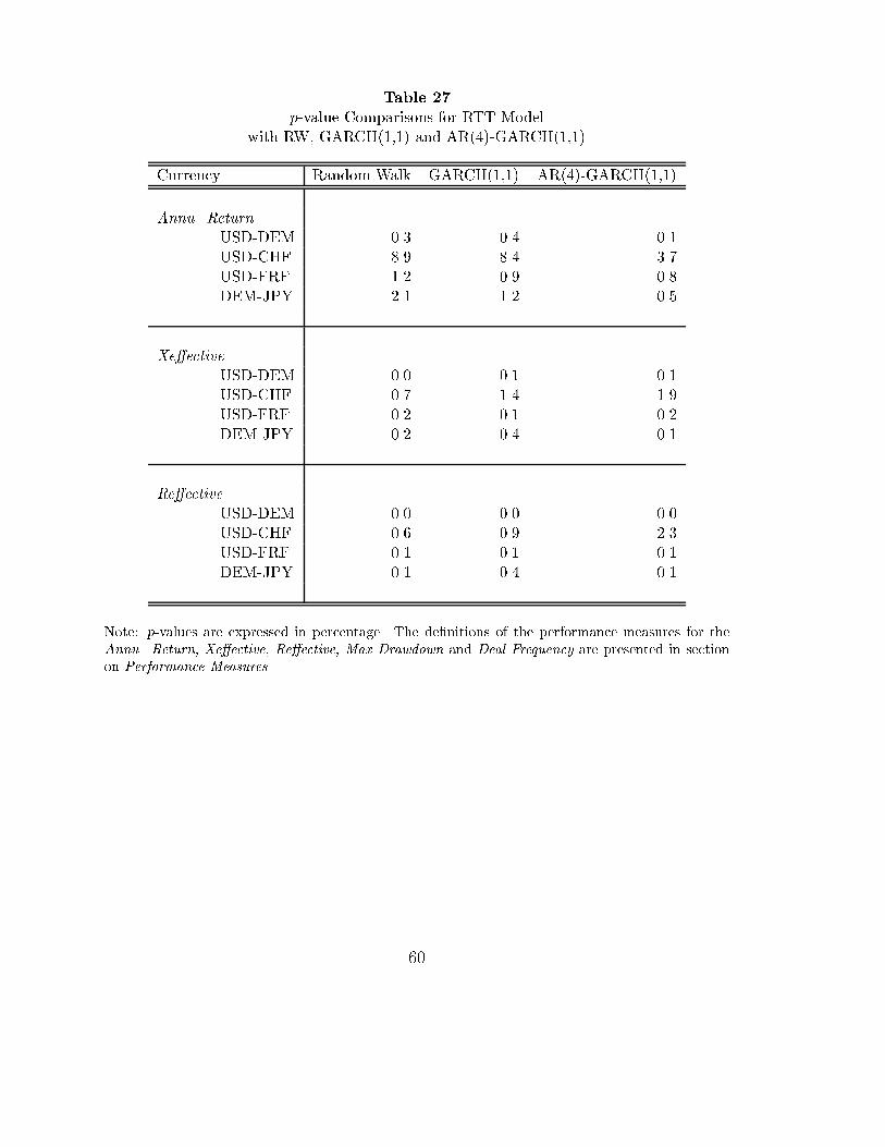
Table 27
p-value Comparisons for RTT Model
with RW, GARCH(1,1) and AR(4)-GARCH(1,1)
Currency Random Walk GARCH(1,1) AR(4)-GARCH(1,1)
Annu. Return
USD-DEM 0.3 0.4 0.1
USD-CHF 8.9 8.4 3.7
USD-FRF 1.2 0.9 0.8
DEM-JPY 2.1 1.2 0.5
Xe�ective
USD-DEM 0.0 0.1 0.1
USD-CHF 0.7 1.4 1.9
USD-FRF 0.2 0.1 0.2
DEM-JPY 0.2 0.4 0.1
Re�ective
USD-DEM 0.0 0.0 0.0
USD-CHF 0.6 0.9 2.3
USD-FRF 0.1 0.1 0.1
DEM-JPY 0.1 0.4 0.1
Note: p-values are expressed in percentage. The de�nitions of the performance measures for the
Annu. Return, Xe�ective, Re�ective, Max Drawdown and Deal Frequency are presented in section
on Performance Measures.
60

Table 28
p-value Comparisons for EMA Model
with RW, GARCH(1,1) and AR(4)-GARCH(1,1)
Currency Random Walk GARCH(1,1) AR(4)-GARCH(1,1)
Annu. Return
USD-DEM 12.6 14.1 10.0
USD-CHF 8.8 9.6 5.9
USD-FRF 6.4 4.6 3.2
DEM-JPY 6.6 2.8 1.8
Xe�ective
USD-DEM 2.8 2.3 3.8
USD-CHF 0.9 0.7 1.7
USD-FRF 0.6 0.6 0.7
DEM-JPY 1.4 0.5 0.5
Re�ective
USD-DEM 2.3 1.8 3.7
USD-CHF 0.4 0.5 2.4
USD-FRF 0.4 0.4 0.6
DEM-JPY 1.0 0.2 0.4
Note: p-values are expressed in percentage. The de�nitions of the performance measures for the
Annu. Return, Xe�ective, Re�ective, Max Drawdown and Deal Frequency are presented in section
on Performance Measures.
61


![Mo delling Elasticit y in Solids using Activ ee b een p erformed using surface mo dels. F or example, Cap onetti et.al. [3] used a surface mo del reconstructed using the o ccluding](https://img.dokumen.tips/doc/110x75/5f5abda6cc564a1c747fdbb1/mo-delling-elasticit-y-in-solids-using-activ-e-e-b-een-p-erformed-using-surface.jpg)