REAL-TIME SCHEDULING FORENERGY HARVESTING SENSOR NODES

C. Moser1, D. Brunelli2, L. Thiele1, L. Benini2

1Computer Engineering and Networks LaboratorySwiss Federal Institute of Technology (ETH) Zurich, Switzerland

2Department of Electronics, Computer Science and SystemsUniversity of Bologna, Italy

Abstract Energy harvesting has recently emerged as a feasible option to increase the oper-ating time of sensor networks. If each node of the network, however, is poweredby a fluctuating energy source, common power management solutions have tobe reconceived. This holds in particular if real-time responsiveness of a givenapplication has to be guaranteed. Task scheduling at the single nodes shouldaccount for the properties of the energy source, capacity of the energy storageas well as deadlines of the single tasks. We show that conventional schedulingalgorithms (like e.g. EDF) are not suitable for this scenario. Based on this mo-tivation, we have constructed optimal scheduling algorithms that jointly handleconstraints from both energy and time domain. Further we present an admittancetest that decides for arbitrary task sets, whether they can be scheduled withoutdeadline violations. To this end, we introduce the concept of energy variabilitycharacterization curves (EVCC) which nicely captures the dynamics of variousenergy sources. Simulation results show that our algorithms allow significantreductions of the battery size compared to Earliest Deadline First scheduling.

1. Introduction

Wireless sensor networks – consisting of numerous tiny sensors that are un-obtrusively embedded in their environment – have been the subject of intensiveresearch. As for many other battery-operated embedded systems, a sensor’soperating time is a crucial design parameter. As electronic systems continueto shrink, however, less energy is storable on-board. Research continues todevelop higher energy-density batteries and supercapacitors, but the amount ofenergy available still severely limits the system’s lifespan. As a result, size aswell as weight of most existing sensor nodes are largely dominated by theirbatteries.

On the other hand, one of the main advantages of wireless sensor networks istheir independence of pre-established infrastructure. That is, in most commonscenarios, recharging or replacing nodes’ batteries is not practical due to (a)inaccessibility and/or (b) sheer number of the sensor nodes. In order for sensornetworks to become a ubiquitous part of our environment, alternative powersources should be employed. Therefore, environmental energy harvesting isdeemed a promising approach: If nodes are equipped with energy transducerslike e.g. solar cells, the generated energy may increase the autonomy of thenodes significantly.

In [14], several technologies have been discussed how, e.g., solar, thermal,kinetic or vibrational energy may be extracted from a node’s physical environ-ment. Moreover, several prototypes (e.g. [2, 5]) have been presented whichdemonstrate both feasibility and usefulness of sensors nodes which are pow-ered by solar or vibrational energy.

From a networking perspective, classical protocols cannot harness the fullpotential provided by the harvesting technology. Here, several publications ex-ist which make routing or clustering decisions within the network harvestingaware [8, 17]. Based on the knowledge of the currently generated power atthe single nodes, the network lifetime can be optimized by shifting the com-munication and computation load. In the example of a solar powered network,nodes which are directly exposed to sunlight have to disburden nodes who arereceiving less radiation due to shadowing effects.

In contrast, we focus on the temporal variations of the energy source expe-rienced by a single node instead of spatial variations between several nodes.The obtained results can e.g. be applied to networks, whose nodes are in-dependently from each other transmitting data to a base station. But even ifwe are dealing with a multi-hop scenario, a single sensor node may need toperform its activities in a timely manner using a limited and uncertain energysource. For example, a node may need to communicate with others by meansof a energy-saving wireless protocol, e.g. by switching on transmitters onlyat well-defined time instances. In addition, there are application scenarios forwhich it is indispensable to fulfill real-time requirements like it is the case in,e.g., fire or intruder detection systems. In general, one can classify real-timeapplication scenarios for wireless sensor networks into safety critical systems,smart spaces as well as entertainment [16]. For all these scenarios, our researchreveals fundamental problems and tradeoffs when real-time behaviour has tobe guaranteed although a sensor’s driving energy source is highly unstable.

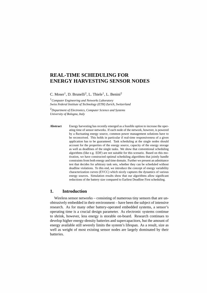
The example in Figure 1 illustrates why greedy scheduling algorithms (likeEarliest Deadline First EDF) are not suitable in the context of regenerative en-ergy. Let us consider a node with an energy harvesting unit that replenishes abattery. For the sake of simplicity, assume that the harvesting unit provides aconstant power output. Now, this node has to perform an arriving task "1" that

stored energy

time

time

task execution

stored energy

time

time

task execution

1 2

12

Figure 1. Greedy vs. lazy scheduling

has to be finished until a certain deadline. Meanwhile, a second task "2" ar-rives that has to respect a deadline which is earlier than the one of task "1". InFigure 1, the arrival times and deadlines of both tasks are indicated by up anddown arrows respectively. As depicted in the top diagrams, a greedy schedul-ing strategy violates the deadline of task "2" since it dispenses overhasty thestored energy by driving task "1". When the energy is required to execute thesecond task, the battery level is not sufficient to meet the deadline. In this ex-ample, however, a scheduling strategy that hesitates to spend energy on task"1" meets both deadlines. The bottom plots illustrate how a Lazy Schedul-ing Algorithm described in this paper outperforms a naive, greedy approachlike EDF in this situation. Lazy scheduling algorithms can be categorized asnon-work conserving scheduling disciplines. Unlike greedy algorithms, a lazyscheduler may be idle although waiting tasks are ready to be processed.

The research presented in this paper is directed towards sensor nodes. Butin general, our results apply for all kind of energy harvesting systems whichmust schedule processes under deadline constraints. For these systems, newscheduling disciplines must be tailored to the energy-driven nature of the prob-lem. This insight originates from the fact, that energy – contrary to the compu-tation resource "time" – is storable. As a consequence, every time we withdrawenergy from the battery to execute a task, we change the state of our schedulingsystem. That is, after having scheduled a first task the next task will encountera lower energy level in the system which in turn will affect its own execu-tion. This is not the case in conventional real-time scheduling where time justelapses either used or unused.

The rest of the paper is organized as follows: In the next section, we high-light the contributions of our work. Subsequently, Section 3 gives definitionsthat are essential for the understanding of the paper. In Section 4, we presentLazy Scheduling Algorithms for optimal online scheduling and proof their op-timality. Admittance tests for arbitrary task sets are the topic of Section 5.Simulation results are presented in Section 6 and Section 7 deals with practicalissues. At the end, Section 8 summarizes related work and Section 9 concludesthe paper.

2. Contributions

The following paper builds on [11] and [12], where Lazy Scheduling Algo-rithms have been presented for the first time. We combine both view points,extend the theoretical results by a formal comparison of the schedulability re-gions of EDF and LSA, include corresponding simulation results as well as adiscussion of implementation aspects. Thereby, we outline how our algorithmscould be implemented on real sensor nodes which illuminates the relevance ofthe proposed theory. The contributions described are as follows:

We present an energy-driven scheduling scenario for a system whoseenergy storage is recharged by an environmental source.

For this scenario, we state and prove optimal online algorithms that dy-namically assign power to arriving tasks. These algorithms are energy-clairvoyant, i.e., scheduling decisions are driven by the knowledge of thefuture incoming energy.

We present an admittance test that decides, whether a set of tasks can bescheduled with the energy produced by the harvesting unit, taking intoaccount both energy and time constraints. For this purpose, we intro-duce the concept of energy variability characterization curves (EVCC).In addition, a formal comparison to EDF scheduling is provided.

By means of simulation, we demonstrate significant capacity savings ofour algorithms compared to the classical EDF algorithm. Finally, weprovide approximations which make our theoretical results applicable topractical energy harvesting systems.

3. System Model

The paper deals with a scheduling scenario depicted in Fig. 2(a). At sometime t, an energy source harvests ambient energy and converts it into electricalpower PS(t). This power can be stored in a device with capacity C. The storedenergy is denoted as EC < C. On the other hand, a computing device drainspower PD(t) from the storage and uses it to process tasks with arrival time ai,

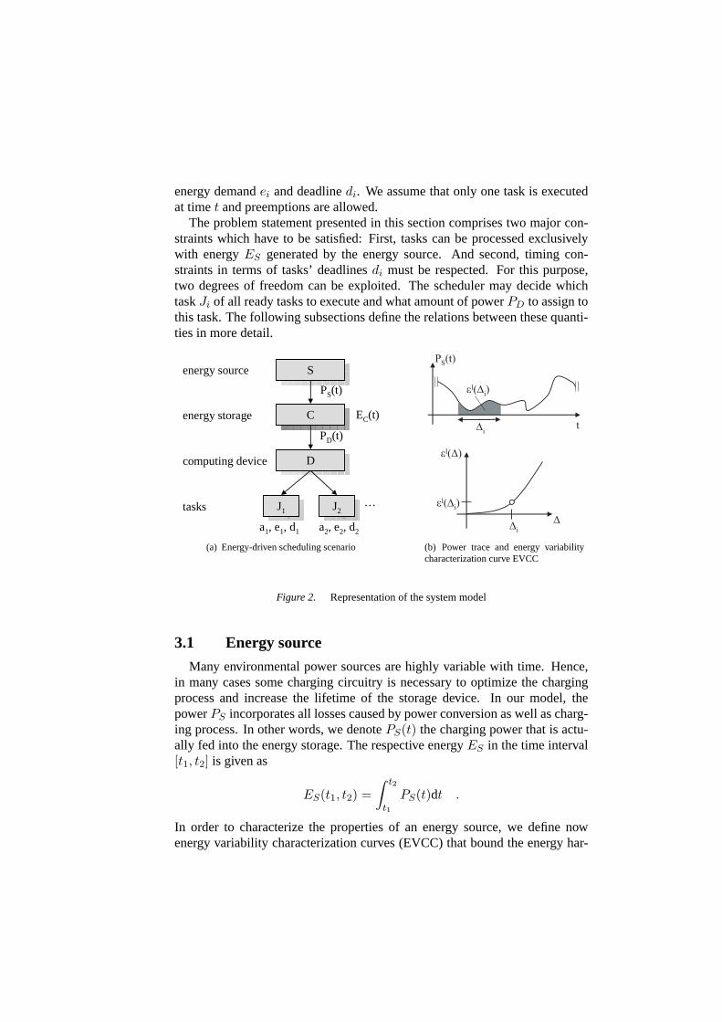
energy demand ei and deadline di. We assume that only one task is executedat time t and preemptions are allowed.

The problem statement presented in this section comprises two major con-straints which have to be satisfied: First, tasks can be processed exclusivelywith energy ES generated by the energy source. And second, timing con-straints in terms of tasks’ deadlines di must be respected. For this purpose,two degrees of freedom can be exploited. The scheduler may decide whichtask Ji of all ready tasks to execute and what amount of power PD to assign tothis task. The following subsections define the relations between these quanti-ties in more detail.

SS

CC

DD

J1J1

energy source

energy storage

computing device

tasks J2J2

…

PS(t)

PD(t)

EC(t)

a1, e1, d1 a2, e2, d2

(a) Energy-driven scheduling scenario

t

PS(t)

Δ

εl(Δ)

Δi

εl(Δi)

Δi

εl(Δi)

(b) Power trace and energy variabilitycharacterization curve EVCC

Figure 2. Representation of the system model

3.1 Energy source

Many environmental power sources are highly variable with time. Hence,in many cases some charging circuitry is necessary to optimize the chargingprocess and increase the lifetime of the storage device. In our model, thepower PS incorporates all losses caused by power conversion as well as charg-ing process. In other words, we denote PS(t) the charging power that is actu-ally fed into the energy storage. The respective energy ES in the time interval[t1, t2] is given as

ES(t1, t2) =∫ t2

t1

PS(t)dt .

In order to characterize the properties of an energy source, we define nowenergy variability characterization curves (EVCC) that bound the energy har-

vested in a certain interval Δ: The EVCCs εl(Δ) and εu(Δ)with Δ ≥ 0 boundthe range of possible energy values ES as follows:

εl(t2 − t1) ≤ ES(t1, t2) ≤ εu(t2 − t1) ∀t2 > t1

Given an energy source, e.g., a solar cell mounted in a building or outside, theEVCCs provide guarantees on the produced energy. For example, the lowercurve denotes that for any time interval of length Δ, the produced energy isat least εl(Δ) (see Fig. 2(b)). Three possible ways of deriving an EVCC for agiven scenario are given below:

A sliding window of length Δ is used to find the minimum/maximumenergy produced by the energy source in any time interval [t1, t2) witht2 − t1 = Δ. To this end, one may use a long power trace or a set oftraces that have been measured. Since the resulting EVCC bounds onlythe underlying traces, these traces must be selected carefully and have tobe representative for the assumed scenario.

The energy source and its environment is formally modeled and the re-sulting EVCC is computed.

Approximations to EVCCs can be determined on-line by using appro-priate measurement and estimation methods, see Section 7.1.

In Section 5, the lower EVCC εl will be used in an admittance test which de-cides, whether a task set is schedulable given a certain energy source. Further-more, both EVCCs will serve as energy predictors for the algorithms simulatedin Section 6.

3.2 Energy storage

We assume an ideal energy storage that may be charged up to its capacityC. According to the scheduling policy used, power PD(t) and the respectiveenergy ED(t1, t2) is drained from the storage to execute tasks. If no tasks areexecuted and the storage is consecutively replenished by the energy source, anenergy overflow occurs. Consequently, we can derive the following constraints

0 ≤ EC(t) ≤ C ∀t

EC(t2) ≤ EC(t1) + ES(t1, t2) − ED(t1, t2) ∀t2 > t1

and therefore

ED(t1, t2) ≤ EC(t1) + ES(t1, t2) ∀t2 > t1 .

3.3 Task scheduling

As illustrated in Fig. 2(a), we utilize the notion of a computing device thatassigns energy EC from the storage to dynamically arriving tasks. We assumethat the power consumption PD(t) is limited by some maximum value Pmax.In other words, the processing device determines at any point in time howmuch power it uses, that is

0 < PD(t) < Pmax .

We assume tasks to be independent from each other and preemptive. Moreprecisely, the currently active task may be preempted at any time and have itsexecution resumed later, at no additional cost. If the node decides to assignpower Pi(t) to the execution of task Ji during the interval [t1, t2], we denotethe corresponding energy

Ei(t1, t2) =∫ t2

t1

Pi(t)dt .

The effective starting time si and finishing time fi of task i are dependent onthe scheduling strategy used: A task starting at time si will finish as soon asthe required amount of energy ei has been consumed by it. We can write

fi = min {t : Ei (si, t) = ei} .

The actual running time (fi − si) of a task i directly depends on the amount ofpower Pi(t) which is driving the task during si ≤ t ≤ fi. At this, the energydemand ei of a task is independent from the power Pi used for its execution.Note that we are not using energy-saving techniques like Dynamic VoltageScaling (DVS), where ei = f(Pi). In our model, power Pi and executiontime wi behave inversely proportional: The higher the power Pi, the shorterthe execution time wi. In the best case, a task may finish after the executiontime wi = ei

Pmaxif it is processed without interrupts and with the maximum

power Pmax.Current hardware technology does not support variable power consumption

as described above. So clearly, the continuous task processing model presentedin this section is idealized. However, a microprocessor for example may step-wise advance a task by switching power on (Pi = Pmax) and off (Pi = 0).By tuning the so-called duty cycle accordingly, devices can approximate theaverage power 0 ≤ P i ≤ Pmax. For a more detailed discussion about practicaltask processing and the system model in general, see Section 7.

4. Lazy Scheduling Algorithms LSA

After having described our modeling assumptions, we will now state andprove optimal scheduling algorithms. In subsection 4.1, we will start with the

analysis of a simplified scheduling scenario where tasks need only energy ascomputation resource but may execute in zero time. By disregarding the com-putation resource time, we focus on the energy-driven nature of the schedulingscenario presented in this paper. In Section 4.2, we will consider finite execu-tion times as well and construct a more general algorithm which manages tooptimally trade off energy and time constraints. Theorems which prove opti-mality of both algorithms will follow in subsection 4.3.

4.1 Simplified Lazy Scheduling

We start with a node with infinite power Pmax = +∞. As a result, a task’sexecution time wi collapses to 0 if the available energy EC in the storage isequal to or greater than the task’s energy demand ei. This fact clearly sim-plifies the search for an adequate scheduling algorithm but at the same timecontributes to the understanding of the problem.

As already indicated in the introduction, the naive approach of simplyscheduling tasks with the EDF algorithm may result in unnecessary deadlineviolations, see Fig. 1. It may happen, that after the execution of task "1" an-other task "2" with an earlier deadline arrives. If now the required energy is notavailable before the deadline of task "2", EDF scheduling produces a deadlineviolation. If task "1" would hesitate instead of executing directly, this deadlineviolation might be avoidable. These considerations directly lead us to the prin-ciple of Lazy Scheduling: Gather environmental energy and process tasks onlyif it is necessary.

The Lazy Scheduling Algorithm LSA-I for Pmax = ∞ shown below at-tempts to schedule a set of tasks Ji, i ∈ Q such that deadlines are respected.Therefore, the processing device has to decide between three power modes.The node may process tasks with the maximal power PD(t) = Pmax or notat all (PD(t) = 0). In between, the node may choose to spend only the cur-rently incoming power PS(t) from the harvesting unit on tasks. The algorithmis based on the three following rules:

Rule 1: If the current time t equals the deadline dj of some arrivedbut not yet finished task Jj , then finish its execution by draining energy(ej − Ej(aj , t)) from the energy storage instantaneously.

Rule 2: We must not waste energy if we could spend it on task execution.Therefore, if we hit the capacity limit (EC(t) = C) at some times t, weexecute the task with the earliest deadline using PD(t) = PS(t).

Rule 3: Rule 1 overrules Rule 2.

Note that LSA-I degenerates to an earliest deadline first (EDF) policy, if C =0. On the other hand, we find an as late as possible (ALAP) policy for the caseof C = +∞.

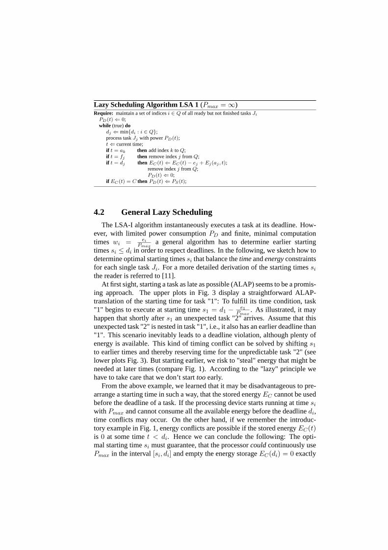
Lazy Scheduling Algorithm LSA 1 (Pmax = ∞)Require: maintain a set of indices i ∈ Q of all ready but not finished tasks Ji

PD(t) ⇐ 0;while (true) do

dj ⇐ min{di : i ∈ Q};process task Jj with power PD(t);t ⇐ current time;if t = ak then add index k to Q;if t = fj then remove index j from Q;if t = dj then EC(t) ⇐ EC(t) − ej + Ej(aj , t);

remove index j from Q;PD(t) ⇐ 0;

if EC(t) = C then PD(t) ⇐ PS(t);

4.2 General Lazy Scheduling

The LSA-I algorithm instantaneously executes a task at its deadline. How-ever, with limited power consumption PD and finite, minimal computationtimes wi = ei

Pmaxa general algorithm has to determine earlier starting

times si ≤ di in order to respect deadlines. In the following, we sketch how todetermine optimal starting times si that balance the time and energy constraintsfor each single task Ji. For a more detailed derivation of the starting times si

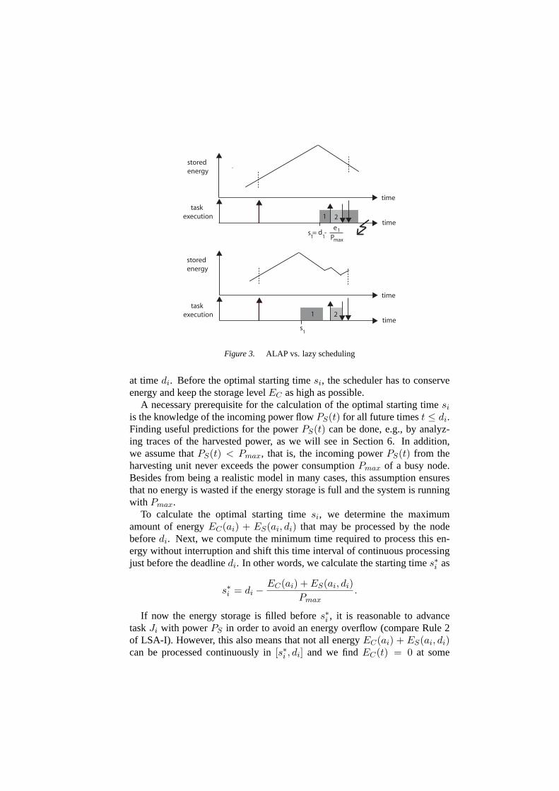
the reader is referred to [11].At first sight, starting a task as late as possible (ALAP) seems to be a promis-

ing approach. The upper plots in Fig. 3 display a straightforward ALAP-translation of the starting time for task "1": To fulfill its time condition, task"1" begins to execute at starting time s1 = d1 − e1

Pmax. As illustrated, it may

happen that shortly after s1 an unexpected task "2" arrives. Assume that thisunexpected task "2" is nested in task "1", i.e., it also has an earlier deadline than"1". This scenario inevitably leads to a deadline violation, although plenty ofenergy is available. This kind of timing conflict can be solved by shifting s1

to earlier times and thereby reserving time for the unpredictable task "2" (seelower plots Fig. 3). But starting earlier, we risk to "steal" energy that might beneeded at later times (compare Fig. 1). According to the "lazy" principle wehave to take care that we don’t start too early.

From the above example, we learned that it may be disadvantageous to pre-arrange a starting time in such a way, that the stored energy EC cannot be usedbefore the deadline of a task. If the processing device starts running at time si

with Pmax and cannot consume all the available energy before the deadline di,time conflicts may occur. On the other hand, if we remember the introduc-tory example in Fig. 1, energy conflicts are possible if the stored energy EC(t)is 0 at some time t < di. Hence we can conclude the following: The opti-mal starting time si must guarantee, that the processor could continuously usePmax in the interval [si, di] and empty the energy storage EC(di) = 0 exactly

stored energy

time

time

task execution 2

stored energy

time

time

task execution 1 2

e1

Pmax

1

s = -11

d

s 1

Figure 3. ALAP vs. lazy scheduling

at time di. Before the optimal starting time si, the scheduler has to conserveenergy and keep the storage level EC as high as possible.

A necessary prerequisite for the calculation of the optimal starting time si

is the knowledge of the incoming power flow PS(t) for all future times t ≤ di.Finding useful predictions for the power PS(t) can be done, e.g., by analyz-ing traces of the harvested power, as we will see in Section 6. In addition,we assume that PS(t) < Pmax, that is, the incoming power PS(t) from theharvesting unit never exceeds the power consumption Pmax of a busy node.Besides from being a realistic model in many cases, this assumption ensuresthat no energy is wasted if the energy storage is full and the system is runningwith Pmax.

To calculate the optimal starting time si, we determine the maximumamount of energy EC(ai) + ES(ai, di) that may be processed by the nodebefore di. Next, we compute the minimum time required to process this en-ergy without interruption and shift this time interval of continuous processingjust before the deadline di. In other words, we calculate the starting time s∗i as

s∗i = di − EC(ai) + ES(ai, di)Pmax

.

If now the energy storage is filled before s∗i , it is reasonable to advancetask Ji with power PS in order to avoid an energy overflow (compare Rule 2of LSA-I). However, this also means that not all energy EC(ai) + ES(ai, di)can be processed continuously in [s∗i , di] and we find EC(t) = 0 at some

time t < di. Thus a better starting time s′i allows for the reduced amount ofenergy C + ES(s′i, di) which is processible in this situation:

s′i = di − C + ES(s′i, di)Pmax

By choosing the maximum of s∗i and s′i we find the optimal starting time

si = max(s′i, s

∗i

),

which precisely balances energy and time constraints for task Ji.The pseudo-code of a general Lazy Scheduling Algorithm LSA-II is shown

below. It is based on the following rules:

Rule 1: EDF scheduling is used at time t for assigning the processor toall waiting tasks with si ≤ t. The currently running task is powered withPD(t) = Pmax.

Rule 2: If there is no waiting task i with si ≤ t and if EC(t) = C,then all incoming power PS is used to process the task with the smallestdeadline (PD(t) = PS(t)).

Lazy Scheduling Algorithm LSA 2 (Pmax = const.)Require: maintain a set of indices i ∈ Q of all ready but not finished tasks Ji

PD(t) ⇐ 0;while (true) do

dj ⇐ min{di : i ∈ Q};calculate sj ;process task Jj with power PD(t);t ⇐ current time;if t = ak then add index k to Q;if t = fj then remove index j from Q;if EC(t) = C then PD(t) ⇐ PS(t);if t ≥ sj then PD(t) ⇐ Pmax;

Although it is based on the knowledge of the future incoming energy ES ,LSA-II remains an online algorithm. The calculation of si must be performedonce the scheduler selects the task with the earliest deadline. If the scheduleris not energy-constraint, i.e., if the available energy is more than the device canconsume with power Pmax within [ai, di], the starting time si will be beforethe current time t. Then, the resulting scheduling policy is EDF, which isreasonable, because only time constraints have to be satisfied. If, however, thesum of stored energy EC plus generated energy ES is small, the schedulingpolicy changes towards an ALAP policy. In doing so, LSA avoids spendingscarce energy on the "wrong" tasks too early.

In summary, LSA-II can be classified as an energy-clairvoyant adaptationof the Earliest Deadline First Algorithm. It changes its behaviour according tothe amount of available energy, the capacity C as well as the maximum powerconsumption Pmax of the device. For example, the lower the power Pmax gets,the greedier LSA-II gets. On the other hand, high values of Pmax force LSA-IIto hesitate and postpone the starting time si. For Pmax = ∞, all starting timescollapse to the respective deadlines, and we identify LSA-I as a special caseof LSA-II. In the remainder of the paper, we will solely consider the generalLSA-II algorithm derived in this section. From now on, we will denote thisalgorithm LSA.

4.3 Optimality of Lazy Scheduling

In this section, we will show that Lazy Scheduling algorithms optimallyassign power PD to a set of tasks. For this purpose, we formulate Theorem1 and Theorem 2 which show that LSA makes the best use of the availabletime and energy, respectively. With the help of Theorem 1 and 2, we proofoptimality of LSA in Theorem 3.

The scheduling scenario presented in this paper is inherently energy-driven.Hence, a scheduling algorithm yields a deadline violation if it fails to assignenergy ei to a task before its deadline di. We distinguish between two types ofdeadline violations:

A deadline cannot be respected since the time is not sufficient to executeavailable energy with power Pmax. At the deadline, unprocessed energyremains in the storage and we have EC(d) > 0. We call this the timelimited case.

A deadline violation occurs because the required energy is simply notavailable at the deadline. At the deadline, the battery is exhausted (i.e.,EC(d) = 0). We denote the latter case energy limited.

For the following theorems to hold we suppose that at initialization of the sys-tem, we have a full capacity, i.e., EC(ti) = C. Furthermore, we call thecomputing device idle if no task i is running with si ≤ t.

Let us first look at the time limited case.

Theorem 1 Let us suppose that the LSA algorithm schedules a set of tasks.At time d the deadline of a task J with arrival time a is missed and EC(d) > 0.Then there exists a time t1 such that the sum of execution times

∑(i) wi =∑

(i)ei

Pmaxof tasks with arrival and deadline within time interval [t1, d] ex-

ceeds d − t1.

Proof 1 Let us suppose that t0 is the maximal time t0 ≤ d where the proces-sor was idle. Clearly, such a time exists.

We now show, that at t0 there is no task i with deadline di ≤ d waiting. Atfirst, note that the processor is constantly operating on tasks in time interval(t0, d]. Suppose now that there are such tasks waiting and task i is actuallythe one with the earliest deadline di among those. Then, as EC(d) > 0 andbecause of the construction of si, we would have si < t0. Therefore, theprocessor would actually process task i at time t0 which is a contradiction tothe idleness.

Because of the same argument, all tasks i arriving after t0 with di ≤ d willhave si ≤ ai. Therefore, LSA will attempt to directly execute them using anEDF strategy.

Now let us determine time t1 ≥ t0 which is the largest time t1 ≤ d suchthat the processor continuously operates on tasks i with di ≤ d. As we havesi ≤ ai for all of these tasks and as the processor operates on tasks withsmaller deadlines first (EDF), it operates in [t1, d] only on tasks with ai ≥ t1and di ≤ d. As there is a deadline violation at time d, we can conclude that∑

(i) wi > d−t1 where the sum is taken over all tasks with arrival and deadlinewithin time interval [t1, d].

It can be shown that a related result holds for the energy limited case, too.

Theorem 2 Let us suppose that the LSA algorithm schedules a set of tasks.At time d the deadline of a task J with arrival time a is missed and EC(d) =0. Assume further, that deadline d is the first deadline of the task set that isviolated by LSA. Then there exists a time t1 such that the sum of task energies∑

(i) ei of tasks with arrival and deadline within time interval [t1, d] exceedsC + ES(t1, d).

Proof 2 Let time t1 ≤ d be the largest time such that (a) EC(t1) = C and(b) there is no task i waiting with di ≤ d. Such a time exists as one couldat least use the initialization time ti with EC(ti) = C. As t1 is the last timeinstance with the above properties, we can conclude that everywhere in timeinterval [t1, d] we either have (a) EC(t) = C and there is some task i waitingwith di ≤ d or we have (b) and EC(t) < C.

It will now be shown that in both cases a) and b), energy is not used toadvance any task j with dj > d in time interval [t1, d]. Note also, that allarriving energy ES(t1, d) is used to advance tasks.

In case a), all non-storable energy (i.e. all energy that arrives from thesource) is used to advance a waiting task, i.e., the one with the earliest deadlinedi ≤ d. In case b), the processor would operate on task J with dj > d if thereis some time t2 ∈ [t1, d] where there is no other task i with di ≤ d waitingand sj ≤ t2. But sj is calculated such that the processor could continuouslywork until dj . As dj > d and EC(d) = 0 this can not happen and sj > t2.Therefore, also in case b) energy is not used to advance any task j with dj > d.

As there is a deadline violation at time d, we can conclude that∑

(i) ei >

C + EC(t1, d) where the sum is taken over all tasks with arrival and deadlinewithin time interval [t1, d].

From the above two theorems we draw the following conclusions: First, in thetime limited case, there exists a time interval before the violated deadline witha larger accumulated computing time request than available time. And sec-ond, in the energy limited case, there exists a time interval before the violateddeadline with a larger accumulated energy request than what can be providedat best. These considerations lead us to one of the major results of the paper:

Theorem 3 (Optimality of Lazy Scheduling) Let us consider asystem characterized by a capacity C and power Pmax driven by the energysource ES . If LSA cannot schedule a given task set, then no other schedulingalgorithm is able to schedule it. This holds even if the other algorithm knowsthe complete task set in advance.

Proof 3 The proof follows immediately from Theorems 1 and 2. Assumea set of tasks is scheduled with LSA and at time d the deadline of task J ismissed. Assume further, that deadline d is the first deadline of the task set thatis violated by LSA. In the following, we distinguish between the case where theenergy at the deadline is EC(d) > 0 and EC(d) = 0, respectively.

In the first case, according to Theorem 1, there exists a time t1 such thatthe sum of execution times

∑(i) wi =

∑(i)

eiPmax

of tasks with arrival anddeadline within time interval [t1, d] exceeds d − t1. Here, knowing arrivaltimes, energy demands and deadlines in advance does not help, since everyscheduling algorithm will at least violate one deadline in [t1, d].

In the energy limited case with EC(d) = 0, according to Theorem 2, thereexists a time t1 such that the sum of task energies

∑(i) ei of tasks with arrival

and deadline within time interval [t1, d] exceeds C + ES(t1, d). Hence, noalgorithm can hold deadline d without violating an earlier deadline in [t1, d].This holds also for omniscient scheduling algorithms, since (a) at the begin-ning of the critical interval [t1, d], the energy level may be EC(t1) = C at mostand (b) the execution of the critical tasks can start at time t1 at the earliest.

So every time LSA violates deadline d, we have either the time limited case(EC(d) > 0) or the energy limited case (EC(d) = 0). Since in both casesit is impossible for another algorithm to respect deadline d and all earlierdeadlines simultaneously, we conclude that LSA is optimal.

If we can guarantee that there is no time interval with a larger accumulatedcomputing time request than available time and no time interval with a largeraccumulated energy request than what can be provided at best, then the taskset is schedulable. This property will be used to determine the admittance testdescribed in the next section.

On the other hand, given a task set and a certain energy source ES(t) we canalso make a statement about the necessary hardware requirements of the sen-sor node: Due to its optimality, LSA requires the minimum processing powerPmax and the minimum capacity C necessary to avoid deadline violations:

Theorem 4 (Optimal tuple (C ; Pmax)) Let us assume a given task sethas to be scheduled using an energy source ES . Among all algorithms, LSArequires the minimum capacity C and the minimum power Pmax that are nec-essary to successfully schedule the task set.

Proof 4 We proceed by contradiction. Let us denote C and Pmax the mini-mum capacity and the minimum processing power which are needed to sched-ule a given task set with LSA. Assume that an adversary algorithm succeedsto schedule the task set with some C ′ < C or P ′

max < Pmax given the sameenergy source. This means the adversary algorithm can schedule the respec-tive task set with (C ′, P ′

max) and LSA cannot. This however contradicts theoptimality of LSA according to Theorem 3.

The admittance test in the next section will allow us to explicitly determinethe minimum values of C and Pmax for LSA scheduling.

5. Admittance Test

5.1 Lazy Scheduling Algorithm

In this section, we will determine an offline schedulability test in case ofperiodic, sporadic or even bursty sets of tasks. In particular, given an energysource with lower EVCC εl(Δ), the device parameters (C ; Pmax) and a set ofperiodic tasks Ji, i ∈ I with period pi, relative deadline di and energy demandei, we would like to determine whether all deadlines can be respected.

To this end, let us first define for each task its arrival curve α(Δ) which de-notes the maximal number of task arrivals in any time interval of length Δ. Theconcept of arrival curves to describe the arrival patterns of sets of tasks is wellknown (request bound functions) and has been used explicitly or implicitlyin, e.g., [4] or [18]. To simplify the discussion, we limit ourselves to periodictasks, but the whole formulation allows to deal with much more general classes(sporadic or bursty) as well.

In case of a periodic task set, we have for periodic task Ji, see also Fig. 4:

αi(Δ) =⌈Δpi

⌉∀Δ ≥ 0

In order to determine the maximal energy demand in any time interval oflength Δ, we need to maximize the accumulated energy of all tasks havingtheir arrival and deadline within an interval of length Δ. To this end, we need

to shift the corresponding arrival curve by the relative deadline. We are do-ing this since the actual energy demand becomes due at the deadline of therespective task. In case of a periodic task Ji, this simply leads to:

αi(Δ) ={

ei · αi(Δ − di) Δ > di

0 0 ≤ Δ ≤ di

In case of several periodic tasks that arrive concurrently, the total demandcurve A(Δ) (called demand-bound function in [4]) can be determined by justadding the individual contributions of each periodic task, see Fig. 4:

A(Δ) =∑i∈I

αi(Δ)

Δ

α1(Δ)

1 2 4 6

12

4

Δ1 2 4 6

24

8

α1 (Δ)α1 (Δ) Α(Δ)

p1 = 2 p1 = 2, d1=1, e1 = 2p

1= 2, d

1=1, e

1= 2

p2

= 3, d2=4, e

2= 1

Δ1 2 4 6

24

8

8

Figure 4. Examples of an arrival curve αi(Δ), a demand curve αi(Δ) and a total demandcurve A(Δ) in case of periodic tasks

Using the above defined quantities, we can formulate a schedulability testfor the LSA algorithm that can be applied to a quite general class of tasksspecifications.

Theorem 5 (LSA Schedulability Test) A given set of tasks Ji, i ∈I with arrival curves αi(Δ), energy demand ei and relative deadline di isschedulable under the energy-driven model with initially stored energy C, ifand only if the following condition holds

A(Δ) ≤ min(εl(Δ) + C , Pmax · Δ

)∀Δ > 0

Here, A(Δ) =∑

i∈I ei · αi(Δ − di) denotes the total energy demand of thetask set in any time interval of length Δ, εl(Δ) the energy variability charac-terization curve of the energy source, C the capacity of the energy storage andPmax the maximal processing power of the system. In case of periodic tasks

we have A(Δ) =∑

i∈I ei ·⌈

Δ−dipi

⌉.

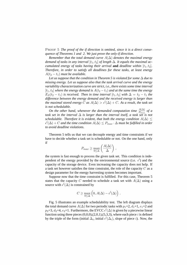
Proof 5 The proof of the if direction is omitted, since it is a direct conse-quence of Theorems 1 and 2. We just prove the only-if direction.

Remember that the total demand curve A(Δ) denotes the maximal energydemand of tasks in any interval [t1, t2] of length Δ. It equals the maximal ac-cumulated energy of tasks having their arrival and deadline within [t1, t2].Therefore, in order to satisfy all deadlines for these tasks, at least energyA(t2 − t1) must be available.

Let us suppose that the condition in Theorem 5 is violated for some Δ due tomissing energy. Let us suppose also that the task arrival curve and the energyvariability characterization curve are strict, i.e., there exists some time interval[t1, t2] where the energy demand is A(t2 − t1) and at the same time the energyES(t2 − t1) is received. Then in time interval [t1, t2] with Δ = t2 − t1 thedifference between the energy demand and the received energy is larger thanthe maximal stored energy C as A(Δ) > εl(Δ) + C. As a result, the task setis not schedulable.

On the other hand, whenever the demanded computation time A(Δ)Pmax

of atask set in the interval Δ is larger than the interval itself, a task set is notschedulable. Therefore it is evident, that both the energy condition A(Δ) ≤εl(Δ) + C and the time condition A(Δ) ≤ Pmax ·Δ must be fulfilled in orderto avoid deadline violations.

Theorem 5 tells us that we can decouple energy and time constraints if wehave to decide whether a task set is schedulable or not. On the one hand, onlyif

Pmax ≥ max0≤Δ

(A(Δ)

Δ

),

the system is fast enough to process the given task set. This condition is inde-pendent of the energy provided by the environmental source (i.e. εl) and thecapacity of the storage device. Even increasing the capacity does not help. Ifa task set however satisfies the time constraint, the role of the capacity C as adesign parameter for the energy harvesting system becomes important.

Suppose now that the time constraint is fulfilled. For this case, Theorem 5states that the capacity C needed to schedule a task set with A(Δ) using asource with εl(Δ) is constrained by

C ≥ max0≤Δ

(0, A(Δ) − εl(Δ)

).

Fig. 5 illustrates an example schedulability test. The left diagram displaysthe total demand curve A(Δ) for two periodic tasks with p1=2, d1=1, e1=2 andp2=3, d2=4, e2=1. Furthermore, the EVCC εl(Δ) is given by a piecewise linearfunction using three pieces (0,0,0),(2,0,1),(5,3,3), where each piece i is definedby the triple of the form (initial Δi, initial εl(Δi), slope of piece i). Now, the

Δ1 2 4 6

24

8

8

ΔPmax. Α(Δ)

Δ1 2 4 6

4

8

8

εl(Δ)

C

Δ1 2 4 6

4

8

8

εl(Δ)

C

E E EΑ(Δ ) Α(Δ)

Figure 5. Determining the optimal tuple (C; Pmax) according to theorem 5

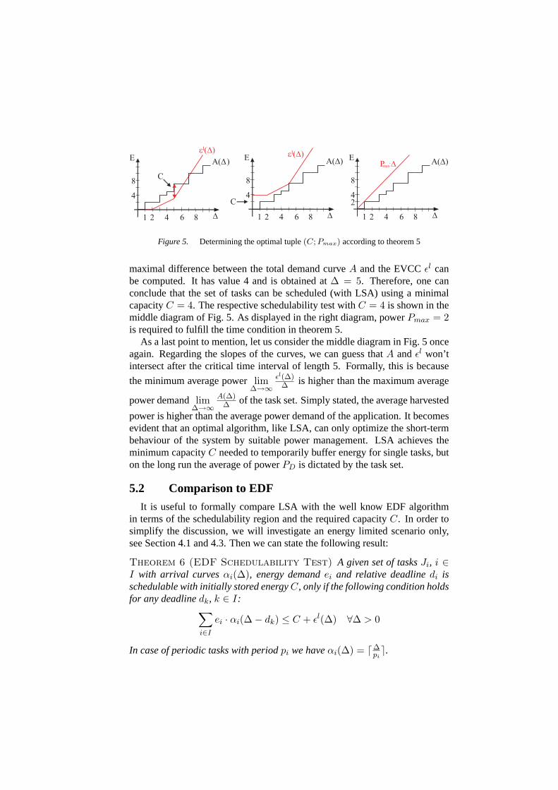
maximal difference between the total demand curve A and the EVCC εl canbe computed. It has value 4 and is obtained at Δ = 5. Therefore, one canconclude that the set of tasks can be scheduled (with LSA) using a minimalcapacity C = 4. The respective schedulability test with C = 4 is shown in themiddle diagram of Fig. 5. As displayed in the right diagram, power Pmax = 2is required to fulfill the time condition in theorem 5.

As a last point to mention, let us consider the middle diagram in Fig. 5 onceagain. Regarding the slopes of the curves, we can guess that A and εl won’tintersect after the critical time interval of length 5. Formally, this is because

the minimum average power limΔ→∞

εl(Δ)Δ is higher than the maximum average

power demand limΔ→∞

A(Δ)Δ of the task set. Simply stated, the average harvested

power is higher than the average power demand of the application. It becomesevident that an optimal algorithm, like LSA, can only optimize the short-termbehaviour of the system by suitable power management. LSA achieves theminimum capacity C needed to temporarily buffer energy for single tasks, buton the long run the average of power PD is dictated by the task set.

5.2 Comparison to EDF

It is useful to formally compare LSA with the well know EDF algorithmin terms of the schedulability region and the required capacity C. In order tosimplify the discussion, we will investigate an energy limited scenario only,see Section 4.1 and 4.3. Then we can state the following result:

Theorem 6 (EDF Schedulability Test) A given set of tasks Ji, i ∈I with arrival curves αi(Δ), energy demand ei and relative deadline di isschedulable with initially stored energy C, only if the following condition holdsfor any deadline dk, k ∈ I:∑

i∈I

ei · αi(Δ − dk) ≤ C + εl(Δ) ∀Δ > 0

In case of periodic tasks with period pi we have αi(Δ) = �Δpi�.

Proof 6 Remember that the left hand side of the condition denotes the max-imal energy used by all the tasks in any interval [t1, t2] of length t2 − t1 =Δ− dk. There is an instance of task arrivals compliant with the arrival curvesαi such that task Jk arrives at time t2, i.e. by correctly adjusting the phaseof all instances of task Jk. In this case, the deadline of the task instance ar-riving at t2 is t2 + dk. In order to be able to execute this instance withinits deadline, the available energy in any interval [t1, t2 + dk] must be largerthan

∑i∈I ei · αi(t2 − t1), i.e. the energy used by tasks arriving in [t1, t2].

The maximal energy available in [t1, t2 + dk] is in the worst case given byC + εl(t2 + dk − t1). Replacing t2 − t1 by Δ − dk yields the desired result.

The strongest bound is obtained by using the task Jk with the smallestdeadline dmin = mini∈J{di}. Comparing Theorems 5 and 6 in the energy-constraint case we obtain the two constraints

∑i∈I ei · αi(Δ − dmin) ≤ C +

εl(Δ) for EDF and∑

i∈I ei·αi(Δ−di) ≤ C+εl(Δ) for LSA. Clearly, EDF hasa smaller schedulability region as

∑i∈I ei·αi(Δ−dmin) ≥ ∑

i∈I ei·αi(Δ−di)for all Δ ≥ 0.

Finally, let us derive specialized results in the case of periodic tasks Ji withpi = di (period equals deadline) and a simple energy variability characteriza-tion curve εl(Δ) shown in Fig. 6 with εl(Δ) = max{σ · (Δ − ρ), 0}.

Δ

εl(Δ)

δ

σ

Figure 6. Simple EVCC for comparing EDF and LSA scheduling

We also suppose that the available average power σ from the energy sourceis sufficient to support the long term power demand σ of the task set

σ ≥ σ =∑i∈I

ei

pi

as otherwise, deadline violations are unavoidable. In the following compar-ison, we suppose that the energy source has a minimal average power, i.e.σ = σ, i.e. it is as weak as possible. Under these assumptions (periodic taskwith periods equal deadlines, energy-limited scenario) and using the results ofTheorems 5 and 6, one can compute the minimal possible capacities of theenergy storage for the two scheduling methods LSA and EDF as follows:

CEDF =∑i∈I

ei + (δ − pmin) · σ ; CLSA = δ · σ

Therefore, the relative gain in the necessary storage capacity between thetwo scheduling methods can be quantified and bounded by

0 ≤ CEDF − CLSA

CLSA=

1δ · σ (

∑i∈I

ei + pmin · σ) ≤ pmax − pmin

δ

For the bounds we use the fact that pmin ≤ (∑

ei)(∑

(ei/pi)) ≤ pmax wherepmin and pmax denote the minimal and maximal period of tasks Ji, respec-tively. In other words, the maximal relative difference in storage capacity de-pends on the differences between the task periods. The larger the differencebetween the largest and smallest period is, the large the potential gain in stor-age efficiency for the LSA algorithm.

6. Simulation Results

In the previous section, a method to compute the minimum capacity for acertain energy source characterization εl was presented. In the following, wewill call this optimal value Cmin. The value Cmin obtained represents a lowerbound since it is obtained for energy-clairvoyant LSA scheduling. In addi-tion, it remains unclear, which capacities C∗

min are required if other schedul-ing disciplines are applied. For this reason, we performed a simulative studyto evaluate the achievable capacity savings in a more realistic scenario. TheEDF algorithm – which is optimal in traditional scheduling theory– serves asa benchmark for our studies.

We investigated variants of LSA which utilize the measured EVCCs εl andεu to predict the future generated energy ES(t) for the LSA algorithm. Eachtime a starting time si has to be calculated for the task i with the earliest dead-line di, the energy εl(di − ai) (or εu(di − ai)) plus the stored energy EC(ai)is assumed to be processible before the deadline.

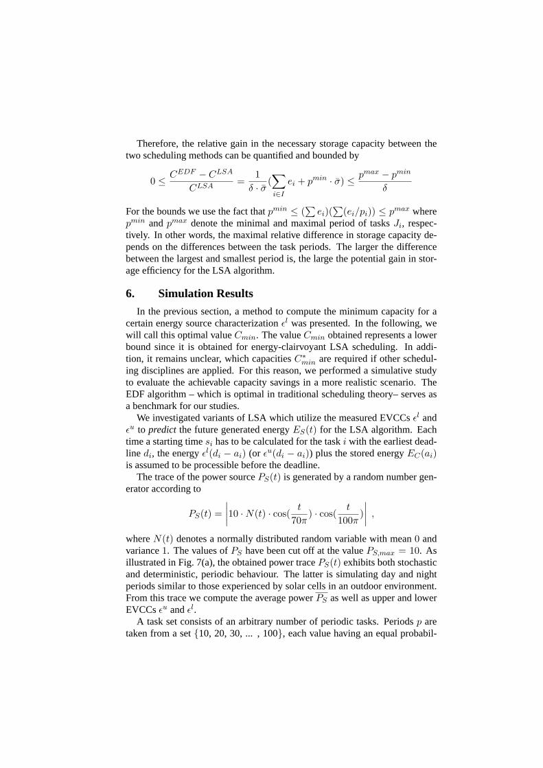
The trace of the power source PS(t) is generated by a random number gen-erator according to

PS(t) =∣∣∣∣10 · N(t) · cos(

t

70π) · cos(

t

100π)∣∣∣∣ ,

where N(t) denotes a normally distributed random variable with mean 0 andvariance 1. The values of PS have been cut off at the value PS,max = 10. Asillustrated in Fig. 7(a), the obtained power trace PS(t) exhibits both stochasticand deterministic, periodic behaviour. The latter is simulating day and nightperiods similar to those experienced by solar cells in an outdoor environment.From this trace we compute the average power PS as well as upper and lowerEVCCs εu and εl.

A task set consists of an arbitrary number of periodic tasks. Periods p aretaken from a set {10, 20, 30, ... , 100}, each value having an equal probabil-

0 1000 2000 3000 4000 50000

1

2

3

4

5

6

7

8

9

10

t

P (t)s

(a) Power trace PS(t)

0 100 200 300 400 500 6000

100

200

300

400

500

600

700

800

Δ

E

A(Δ)

ε (Δ)l

Cmin

(b) Determining Cmin for a random task set

Figure 7. Calculation of Cmin in two steps: (1) Extract εl(Δ) from PS(t) and (2) ComputeCmin for every task set with respective energy demand A(Δ)

ity of being selected. The initial phases ϕ are uniformly distributed between[0,100]. For simplicity, the relative deadline d is equal to the period p of thetask. The energies e of the periodic tasks are generated according to a uniformdistribution in [0, emax], with emax = PS · p.

We define the utilization U ∈ [0, 1] of a scheduler as

U =∑

i

ei

PS

pi.

One can interpret U as the percentage of processing time of the device if tasksare solely executed with the average incoming power PS . A system with, e.g.,U > 1 is processing more energy than it scavenges on average and will depleteits energy reservoir.

In dependence of the generated power source PS(t), N task sets are gener-ated which yield a certain processor utilization U . For that purpose, the numberof periodic tasks in each task set is successively incremented until the intendedutilization U is reached. Hence, the accuracy of the utilization U is varying±1% with respect to its nominal value.

At the beginning of the simulation, the energy storage is full. We set Pmax =10. The simulation terminates after 10000 time units and is repeated for 5000task sets. In order to show the average behaviour of all task sets in one plot, wenormalized the capacities C with the respective Cmin of the task set. Fig. 7(b)shows the calculation of Cmin for a random task set.

Fig. 8 illustrates the percentage of tasks that could be scheduled withoutdeadline violations for different utilizations U . Clearly, no deadline violationsoccur for energy-clairvoyant LSA scheduling and values of C

Cmin≥ 1. For all

values of U , both approximations of LSA with εl and εu outperform the EDF

1 1.1 1.2 1.3 1.4 1.5 1.75 20

20

40

60

80

100

]

1 1.1 1.2 1.3 1.4 1.5 1.75 20

20

40

60

80

100

perc

enta

ge o

f pas

sed

task

s

C/C min

U=40%

LSA E (t)ε

EDF

ls

1 1.1 1.2 1.3 1.4 1.5 1.75 20

20

40

60

80

100

1 1.1 1.2 1.3 1.4 1.5 1.75 20

20

40

60

80

100

LSALSA

U=20%

U=60% U=80%

C/C minC/C min

perc

enta

ge o

f pas

sed

task

s

perc

enta

ge o

f pas

sed

task

s

perc

enta

ge o

f pas

sed

task

s

C/C min

LSA E (t)ε

EDF

ls

LSALSA

LSA E (t)ε

EDF

ls

LSALSA

LSA E (t)εε

EDF

l

u

sLSALSA

εuεu

εu

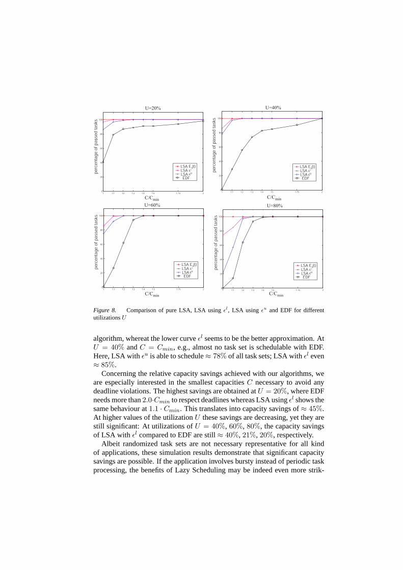
Figure 8. Comparison of pure LSA, LSA using εl, LSA using εu and EDF for differentutilizations U

algorithm, whereat the lower curve εl seems to be the better approximation. AtU = 40% and C = Cmin, e.g., almost no task set is schedulable with EDF.Here, LSA with εu is able to schedule ≈ 78% of all task sets; LSA with εl even≈ 85%.

Concerning the relative capacity savings achieved with our algorithms, weare especially interested in the smallest capacities C necessary to avoid anydeadline violations. The highest savings are obtained at U = 20%, where EDFneeds more than 2.0·Cmin to respect deadlines whereas LSA using εl shows thesame behaviour at 1.1 · Cmin. This translates into capacity savings of ≈ 45%.At higher values of the utilization U these savings are decreasing, yet they arestill significant: At utilizations of U = 40%, 60%, 80%, the capacity savingsof LSA with εl compared to EDF are still ≈ 40%, 21%, 20%, respectively.

Albeit randomized task sets are not necessary representative for all kindof applications, these simulation results demonstrate that significant capacitysavings are possible. If the application involves bursty instead of periodic taskprocessing, the benefits of Lazy Scheduling may be indeed even more strik-

ing: As showed in [11], a greedy algorithm like EDF may violate an arbitrarynumber of deadlines and may suffer from worst case scenarios. This holds inparticular for sensor nodes, where the energy demands of different tasks arehighly varying (e.g. communication, sensing and data processing tasks) andtasks have to satisfy various timing constraints (e.g. urgent and less urgenttasks which have to run in parallel).

7. Practical Considerations

The system model introduced in Section 3 and used throughout this paperimplies idealized modelling abstractions, which demand further explanations.Therefore, this section is dedicated to general implementation aspects and pos-sible application scenarios

7.1 Energy Source Predictability

Clearly, the performance of LSA is strongly dependent on the accuracy ofthe predicted power PS(t) of the harvesting unit. The better the approxima-tion, the better the algorithm performs in terms of optimality. As illustrated bythe simulation results of the previous section, energy variability characteriza-tion curves (EVCC) are suitable for that purpose. Especially for small utiliza-tions U of the sensor node, EVCCs appear to converge towards the optimal,energy-clairvoyant LSA. It should be mentioned, that the prediction of ES(t)by EVCCs may even be improved if the sensor node is learning the character-istics of the energy source adaptively: By observing energy values ES(Δ′) forpast intervals Δ′, the prediction for future intervals Δ can be optimized online.This extension, however, increases at the same time the computational demandof the scheduler, which is one of the advantages of using simple EVCCs.

Solar energy harvesting through photovoltaic conversion is deemed a num-ber one candidate for the power source PS described in our model. If weassume the sensor node to be placed in an outdoor environment, the impingingradiation is variable with time, but follows a diurnal as well as annual cycle.Moreover, during short time intervals, the produced power PS can be regardedas constant and sudden changes of the light intensity are improbable. Due tothis specific nature of solar energy, a two-tiered prediction methodology is self-evident: On the one hand, long-run predictions must be made for less urgenttasks with rather late deadlines. Here, using exponential decaying factors toweight the history of recorded powers PS is one possibility. An alternativeis to combine daily and seasonal light conditions of the past with the knowl-edge about a sensor’s environment and possible shadowing. One can think ofa plurality of prediction mechanisms, which are clearly out of the scope of thispaper.

For urgent tasks with close deadlines within milliseconds or seconds, intelli-gent prediction algorithms may not be necessary. Here, tasks like, e.g., sendinga few bits over the wireless channel may be planned assuming constant powerPS(t) = PS,const during si ≤ t ≤ di. For stationarity of the power inflow PS

the calculation of the starting time si for a task i simplifies to

si = di − min(

EC(ai) + (di − ai)PS,const

Pmax,

C

Pmax − PS,const

).

In the worst case, a sensor node is powered by an energy source with purestochastic behaviour. If nothing is known about this source, the currently storedenergy ES is the only indicator for making scheduling decisions. By iterativelyupdating the starting time si = di − EC(t)

Pmax(and thereby increasing the com-

putational overhead) starting task i too early can be avoided. However, oncethe device is running with Pmax, the incoming energy ES(si, di) may not beprocessible in the remaining interval [si, di]. Consequently, optimality cannotbe guaranteed for this scenario since the starting time si is always earlier thenthe optimal starting time si.

7.2 Task Processing

The task processing model presented in this paper exhibits two major as-sumptions:

1 We assume the power PD(t) driving a task to be continuously adjustablewith respect to its value in [0; Pmax] as well as with respect to time t.That is, at any point in time a task can be advanced with an accuratelydefined amount of power.

2 We assume a linear relationship between the power PD used for execut-ing a task and the execution time w. We can say: the higher the powerPD, the shorter the execution time w.

The first modelling assumption is only needed in situations when the energystorage is full (EC(t) = C). In practice, there is no existing hardware thatsupports a continuous consumption of the scavenged power PS(t) as claimedby LSA. A microcontroller, e.g., drains roughly constant power from the bat-tery when running a piece of program. The same holds for the radio interface.When transmitting a certain amount of data, most radios won’t operate prop-erly with unstable power supply. Therefore, we assume that the respectivehardware attempts to approximate the power level of the power source by con-tinuously switching power on (PD = Pmax) and off (PD = 0). In Fig. 9, theachieved average power PD ≈ PS is sketched.

It becomes evident that in an implementation, one will have to respect a cer-tain granularity. The scheduler needs to determine when the energy storage is

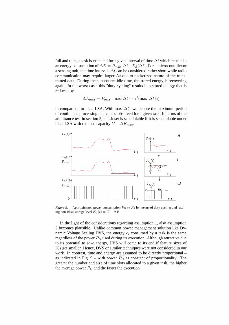
full and then, a task is executed for a given interval of time Δt which results inan energy consumption of ΔE = Pmax ·Δt−ES(Δt). For a microcontoller ora sensing unit, the time intervals Δt can be considered rather short while radiocommunication may require larger Δt due to packetized nature of the trans-mitted data. During the subsequent idle time, the stored energy is recoveringagain. In the worst case, this "duty cycling" results in a stored energy that isreduced by

ΔEmax = Pmax · max{Δt} − εl(max{Δt}))

in comparison to ideal LSA. With max{Δt} we denote the maximum periodof continuous processing that can be observed for a given task. In terms of theadmittance test in section 5, a task set is schedulable if it is schedulable underideal LSA with reduced capacity C − ΔEmax.

Figure 9. Approximated power consumption PD ≈ PS by means of duty cycling and result-ing non-ideal storage level EC(t) = C − ΔE

In the light of the considerations regarding assumption 1, also assumption2 becomes plausible. Unlike common power management solution like Dy-namic Voltage Scaling DVS, the energy ei consumed by a task is the sameregardless of the power PD used during its execution. Although attractive dueto its potential to save energy, DVS will come to its end if feature sizes ofICs get smaller. Hence, DVS or similar techniques were not considered in ourwork. In contrast, time and energy are assumed to be directly proportional –as indicated in Fig. 9 – with power PD as constant of proportionality. Thegreater the number and size of time slots allocated to a given task, the higherthe average power PD and the faster the execution.

7.3 Energy Storage Model

An important step for the validation of the theory presented in this paperis the discussion of the energy storage model. Looking at the various devicesavailable on the market, there are two principal methods to store energy in asmall volume or mass device: using an electro-chemical process or just per-forming physical separation of electrical charges across a dielectric medium.The first technique is used by rechargeable batteries and it is currently the mostcommon and for long time it was the only method to achieve high capacitiesin a small size. Nevertheless, research in the last years has found new mate-rials in order to increase the specific energy of capacitors, producing devicesthat are called supercapacitor or ultra-capacitor [7]. As shown in the so-called’Ragone plot’ in Fig. 10, supercapacitors offer a trade-off between power- aswell as energy-density, filling the gap between batteries and capacitors. Be-yond their ability to support higher power flows than batteries, supercapacitorsovercome many other drawbacks of batteries: They have very long lifetimesand tolerate an almost unlimited number of charge/recharge cycles withoutperformance degradation. Unlike batteries, no heat is released during charg-ing/discharging due to parasitic, chemical reactions. In the following, we willfocus on supercapacitors as possible candidates for an energy storage device.

Power Density (W/Kg)

En

erg

y

Den

sity

(J/

Kg

)

Electrolytics

Capacitors

NI-CD

NI-MH

LI-ion

Super-capacitorsLead-acid

Figure 10. Power and energy characteristics of storage devices

Charge retention. Self-discharging is a natural phenomena that occurs inall kind of storage devices. It is caused by leakage currents that flow insidethe device discharging it. Supercapacitors exhibit leakage currents that aretypically in the order of magnitude of μA (see e.g. [9]). Moreover, it shouldbe mentioned that the leakage is proportional to the energy level. In [5], the

leakage behaviour of different supercapacitors have been tested. From Fig.2 inthe latter work it becomes evident, that there exist a potential to minimize theleakage of fully charged supercapacitors by appropriate choice (manufacturertechnology) and arrangement (serial, parallel) of devices.

Apart from the intrinsic energy leakage of supercapacitors, also the idlepower consumption of the sensor node has to be considered. This "externalleakage" can be reduced by switching to a low-power mode if no tasks areexecuted. In case of a low power wireless sensor node like Moteiv’s TmoteSky [10], its ultra low power Texas Instruments MSP430 F1611 microcon-troller exhibits a maximum current of 3.0μA in low power mode (LPM3). Thewakeup to active mode is finished after 6μs.

Altogether, it can be assumed that the energy conservation laws describedin Section 3.2 hold and introducing an additional term allowing for energyleakage is dispensable.

Monitoring the stored energy. An important feature of energy harvest-ing systems is the capability to estimate the remaining energy in the storagedevice. Unlike batteries, the energy of supercapacitors can be measured in astraightforward way: The equations describing the physical behaviour of su-percapacitors are nearly the same as the ones for ordinary capacitors, and theenergy stored is hence EC ≈ 1

2CV 2.

Storage efficiency. The efficiency η of a supercapacitor can be regardedas the quantity that relates the power flows and energies displayed in Fig. 10.Since charging a supercapacitor with PS and discharging it with PD can beseen as symmetrical operations, let us consider the efficiency η when the su-percapacitor is charged. In this case, the increment of stored energy in timeinterval Δ = t2 − t1 can be written as

EC(t2) − EC(t1) =∫ t2

t1

PS(t)dt = η

∫ t2

t1

PS,raw(t)dt ,

where PS,raw denotes the power fed into the supercapacitor. In general, super-capacitors may suffer from low efficiencies η due to their high equivalent seriesresistance [3]. This circumstance, however, does not jeopardize our modelingassumptions as such since, as stated in section 3.1, all losses are included inthe definition of PS . Actually, the more important property of the efficiency ηis its independence of the energy level EC(t) at time t, which is approximatelytrue for supercapacitors. Moreover, supercapacitors barely produce thermalheat which could reinforce non-linear charging/discharging behaviour.

In summary, we conclude that a linear charging/discharging behaviour withconstant efficiency η is a reasonable abstraction for the example of a super-capacitor and hence our modeling assumptions hold. It should be mentioned,

that possible variations of the efficiency η have been disregarded in relatedwork like [5] and [6], too.

8. Related Work

In [6], the authors use a similar model of the power source as we do. Butinstead of executing concrete tasks in a real-time fashion, they propose tuninga node’s duty cycle dependent on the parameters of the power source. Nodesswitch between active and sleep mode and try to achieve sustainable oper-ation. This approach only indirectly addresses real-time responsiveness: Itdetermines the latency resulting from the sleep duration.

The approach in [15] is restricted to a very special offline scheduling prob-lem: Periodic tasks with certain rewards are scheduled within their deadlinesaccording to a given energy budget. The overall goal is to maximize the sumof rewards. Therefore, energy savings are achieved using Dynamic VoltageScaling (DVS). The energy source is assumed to be solar and comprises twosimple states: day and night. Hence the authors conclude that the capacity ofthe battery must be at least equal to the cumulated energy of those tasks, thathave to be executed at night. In contrast, our work deals with a much moredetailed model of the energy source. We focus on scheduling decisions forthe online case when the scheduler is indeed energy-constraint. In doing so,we derive valuable bounds on the necessary battery size for arbitrary energysources and task sets.

The research presented in [1] is dedicated to offline algorithms for schedul-ing a set of periodic tasks with a common deadline. Within this so-called"frames", the order of task execution is not crucial for whether the task set isschedulable or not. The power scavenged by the energy source is assumed tobe constant. Again – by using DVS – the energy consumption is minimizedwhile still respecting deadlines. Contrary to this work, our systems (e.g. sen-sor nodes) are predominantly energy constrained and the energy demand ofthe tasks is fixed (no DVS). We propose algorithms that make best use of theavailable energy. Provided that the average harvested power is sufficient forcontinuous operation, our algorithms minimize the necessary battery capacity.

The primary commonality of [13] and our work is the term "lazy schedul-ing". In [13], lazy packet scheduling algorithms for transmitting packetizedinformation in a wireless network are discussed. The approach is based on theobservation that many channel coding schemes allow to reduce the energy perpacket if it is transmitted slower, i.e. over a longer duration. Goal of this ap-proach is to minimize the energy, whereas in our work the energy consumptionis fixed (given by the task set). Furthermore, their scheduling algorithms arefully work conserving, which is not true for our algorithms.

9. Conclusions

We studied the case of an energy harvesting sensor node that has to schedulea set of tasks with real-time constraints. The arrival times, energy demands anddeadlines of the tasks are not known to the node in advance and the problemconsists of assigning the right amount of power in the right order to those tasks.For this purpose, we constructed optimal Lazy Scheduling Algorithms LSAwhich are energy-clairvoyant, i.e., the generated energy in the future is known.Contrary to greedy scheduling algorithms, LSA hesitates to power tasks untilit is necessary to respect timing constraints. As a further result, we discussan admittance test that decides, whether a set of energy-driven tasks can bescheduled on a sensor node without violating deadlines. This admittance testsimultaneously shads light on the fundamental question of how to dimensionthe capacity of the energy storage: Provided that the average harvested poweris sufficient for continuous operation, we are able to determine the minimumbattery capacity necessary. Furthermore, achievable capacity savings between20% and 45% are demonstrated in a simulative study, comparing the classi-cal Earliest Deadline First algorithm with a variant of LSA, which uses energyvariability characterization curves EVCC as energy predictor. Finally, practicalconsiderations are provided that suggest practical applicability of the theoreti-cal results.

By starting to study a single node, we believe that extensions towards mul-tihop networks where end-to-end deadlines have to be respected are possible.If sensors jointly perform a common sensing task, distributed energy manage-ment solutions are needed. An example for the common task could be redun-dantly deployed sensors with overlapping coverage regions.

Acknowledgments

The work presented in this paper was partially supported by the NationalCompetence Center in Research on Mobile Information and CommunicationSystems (NCCR-MICS), a center supported by the Swiss National ScienceFoundation under grant number 5005-67322. In addition, this research hasbeen founded by the European Network of Excellence ARTIST2.

References[1] A. Allavena and D. Mosse. Scheduling of frame-based embedded systems with recharge-

able batteries. In Workshop on Power Management for Real-Time and Embedded Systems(in conjunction with RTAS 2001), 2001.

[2] Y. Ammar, A. Buhrig, M. Marzencki, B. Charlot, S. Basrour, K. Matou, and M. Renaudin.Wireless sensor network node with asynchronous architecture and vibration harvestingmicro power generator. In sOc-EUSAI ’05: Proceedings of the 2005 joint conferenceon Smart objects and ambient intelligence, pages 287–292, New York, NY, USA, 2005.ACM Press.

[3] P. Barrade and A. Rufer. Current capability and power density of supercapacitors: Con-siderations on energy efficiency. In European Conference on Power Electronics andApplications (EPE), 2003, Toulouse, France, September 2-4 2003.

[4] S. K. Baruah. Dynamic- and static-priority scheduling of recurring real-time tasks. Real-Time Systems, 24(1):93–128, 2003.

[5] X. Jiang, J. Polastre, and D. E. Culler. Perpetual environmentally powered sensor net-works. In Proceedings of the Fourth International Symposium on Information Processingin Sensor Networks, IPSN 2005, pages 463–468, UCLA, Los Angeles, California, USA,April 25-27 2005.

[6] A. Kansal, D. Potter, and M. B. Srivastava. Performance aware tasking for environ-mentally powered sensor networks. In Proceedings of the International Conference onMeasurements and Modeling of Computer Systems, SIGMETRICS 2004, pages 223–234,New York, NY, USA, June 10-14 2004. ACM Press.

[7] R. Kötz and M. Carlen. Principles and applications of electrochemical capacitors. InElectrochimica Acta 45, pages 2483–2498. Elsevier Science Ltd., 2000.

[8] L. Lin, N. B. Shroff, and R.Srikant. Asymptotically optimal power-aware routing formultihop wireless networks with renewable energy sources. In Proceedings of IEEEINFOCOM 2005, pages 1262 – 1272, Miami, USA, March 13-17 2005.

[9] Maxwell technologies, Inc. Boostcap ultracapacitor - pc series data sheet.http://www.maxwell.com/pdf/uc/datasheets/PC Series.pdf, June, 2006.

[10] Moteiv Corporation. Tmote sky - ultra low power ieee 802.15.4 compliant wireless sen-sor module, datasheet. http://www.moteiv.com/products/docs/tmote-sky-datasheet.pdf,June, 2006.

[11] C. Moser, D. Brunelli, L. Thiele, and L. Benini. Lazy scheduling for energy-harvestingsensor nodes. In Fifth Working Conference on Distributed and Parallel Embedded Sys-tems, DIPES 2006, pages 125–134, Braga, Portugal, October 11-13 2006.

[12] C. Moser, D. Brunelli, L. Thiele, and L. Benini. Real-time scheduling with regenerativeenergy. In Proc. of the 18th Euromicro Conference on Real-Time Systems (ECRTS 06),pages 261–270, Dresden, Germany, July 2006.

[13] B. Prabhakar, E. Uysal-Biyikoglu, and A. E. Gamal. Energy-efficient transmission overa wireless link via lazy packet scheduling. In INFOCOM 2001. Twentieth Annual JointConference of the IEEE Computer and Communications Societies. Proceedings. IEEE,pages 386–394, Anchorage, AK, USA, April 2001.

[14] S. Roundy, D. Steingart, L. Frechette, P. K. Wright, and J. M. Rabaey. Power sources forwireless sensor networks. In Wireless Sensor Networks, First European Workshop, EWSN2004, Proceedings, Lecture Notes in Computer Science, pages 1–17, Berlin, Germany,January 19-21 2004. Springer.

[15] C. Rusu, R. G. Melhem, and D. Mosse. Multi-version scheduling in rechargeable energy-aware real-time systems. In 15th Euromicro Conference on Real-Time Systems, ECRTS2003, pages 95–104, Porto, Portugal, July 2-4 2003.

[16] J. Stankovic, T. Abdelzaher, C. Lu, L. Sha, and J. Hou. Real-time communication andcoordination in embedded sensor networks. In Proceedings of the IEEE, vol.91, no.7pp.1002- 1022, July 2003.

[17] T. Voigt, H. Ritter, J. Schiller, A. Dunkels, and J. Alonso. Solar-aware clustering inwireless sensor networks. In Proceedings of the Ninth IEEE Symposium on Computersand Communications, June 2004.

[18] E. Wandeler, A. Maxiaguine, and L. Thiele. Quantitative characterization of eventstreams in analysis of hard real-time applications. Real-Time Systems, Springer Sci-ence+Business Media B.V., 9(2):205–225, 2005.

Clemens Moser is a Ph.D. student at the Computer Engi-

neering and Networks Laboratory of the Swiss Federal In-

stitute of Technology, Zurich. His research interests include

design, analysis and optimization of energy harvesting sensor

networks. He studied electrical engineering and information

technology at the Technical University of Munich, where he

received the B.Sc. and Dipl.Ing. degree in 2003 and 2004, re-

spectively. For his diploma thesis in 2004, he joined DoCoMo

Euro-Labs to work on topology aspects of wireless multihop

networks.

Davide Brunelli is currently pursuing the PhD degree at the

University of Bologna, Italy. He received the electrical en-

gineering degree from the University of Bologna, in 2002.

His research interests concern design and analysis of wireless

sensor networks for ambient intelligence and ubiquitous com-

puting, with particular emphasis on energy scavenging tech-

niques.

Lothar Thiele joined ETH Zurich, Switzerland, as a full

Professor of Computer Engineering, in 1994. He is leading

the Computer Engineering and Networks Laboratory of ETH

Zurich. His research interests include models, methods and

software tools for the design of embedded systems, embedded

software and bioinspired optimization techniques. In 1986,

he received the "Dissertation Award" of the Technical Uni-

versity of Munich, in 1987, the "Outstanding Young Author

Award" of the IEEE Circuits and Systems Society, in 1988,

the Browder J. Thompson Memorial Award of the IEEE, and

in 2000-2001, the "IBM Faculty Partnership Award". In 2004,

he joined the German Academy of Natural Scientists Leopold-

ina. In 2005, he was the recipient of the Honorary Blaise Pas-

cal Chair of University Leiden, The Netherlands.

Luca Benini is an Full Professor at the University of Bologna.

He also holds a visiting faculty position at the Ecole Polytec-

nique Federale de Lausanne (EPFL). Dr. Benini’s research in-

terests are in the design of systems for ambient intelligence,

from multi-processor systems-on-chip/networks on chip to

energy-efficient smart sensors and sensor networks. He has

published more than 350 papers in peer-reviewed international

journals and conferences, three books, several book chapters

and two patents. He has been program chair and vice-chair of

Design Automation and Test in Europe Conference. He is As-

sociate Editor of the IEEE Transactions on Computer-Aided

Design of Circuits and Systems and of the ACM Journal on

Emerging Technologies in Computing Systems. He is a Fel-

low of the IEEE.