Real-time sampling of Ground Penetrating Radar and Related

2005:039 CIV

M A S T E R ' S T H E S I S

Real-time Sampling ofGround Penetrating Radar

and Related Processing

Nils Björklund Tore Johnsson

Luleå University of Technology

MSc Program in Engineering

Department of Computer Science and Electrical EngineeringDivision of Signal Processing

2005:039 CIV - ISSN: 1402-1617 - ISRN: LTU-EX--05/039--SE

Real-time Sampling of GroundPenetrating Radar and Related

Processing

Nils Bj orklundTore Johnsson

Lulea University of TechnologyDept. of Computer Science and Electrical Engineering

Division of Signal Processing

January 17, 2005

ii

ABSTRACT

Ground penetrating radar (GPR) is a technique for inspecting objects and surfaces hidden underobstructing materials. Common uses are inspections of the bedrock, ground water and otherlayers in the ground. It can also be used for short distance investigations where high precisionis needed, such as in road quality examinations.

As with all radar systems, relatively high frequency electromagnetic waves are used inranges of 40 MHz up to several GHz. To get the resulting data in digital form, as almostalways needed because of recording and postprocessing needs, analog to digital conversionmust be performed. Sampling and converting such high frequency signals requires a veryhigh sampling frequency, so high that common real-time sampling techniques have not beenpossible to use. Instead a technique, called time equivalent sampling, that reduces the neededsampling frequency dramatically has been used. The disadvantage of time equivalent samplingis the low speed. Recently, the ever progressing development of faster electronics has madeconverters with high sampling frequencies, adequate for GPR use, available.

Real-time sampling of GPR opens for new signal processing possibilities, the main onebeing stacking of the signal. Stacking is a technique for lowering the noise of the receivedradar reflections, and could lead to a longer range for GPR systems.

In this project, the main objective was to investigate the possibilities of performing real-time sampling, and related processing, with standard electronic hardware. In the end a proto-type real-time sampling GPR system was developed. It can stack up to 3000 GPR-scans persecond, and also perform filtering and other processing. As this was only a prototype, codeefficiency was not a high priority and therefore a noticeable speed increase is probable afteroptimization.

iii

iv

CONTENTSCHAPTER 1: INTRODUCTION 3

1.1 Introduction to ground penetrating radar . . . . . . . . . . . . . . . . . . . . . 31.2 Capturing data from GPR . . . . . . . . . . . . . . . . . . . . . . . . . . . . . 61.3 GPR Processing . . . . . . . . . . . . . . . . . . . . . . . . . . . . . . . . . . 81.4 Project objective . . . . . . . . . . . . . . . . . . . . . . . . . . . . . . . . . 9

CHAPTER 2: METHOD AND RESULTS 112.1 Hardware overview . . . . . . . . . . . . . . . . . . . . . . . . . . . . . . . . 112.2 DSP Software . . . . . . . . . . . . . . . . . . . . . . . . . . . . . . . . . . . 132.3 PC Software . . . . . . . . . . . . . . . . . . . . . . . . . . . . . . . . . . . . 192.4 Results . . . . . . . . . . . . . . . . . . . . . . . . . . . . . . . . . . . . . . . 20

CHAPTER 3: CONCLUSIONS 25

APPENDIX A: A BBREVIATIONS 27

vi

L IST OF FIGURES1.1 Different radar methods used in GPR. . . . . . . . . . . . . . . . . . . . . . . 41.2 Time equivalent sampling. . . . . . . . . . . . . . . . . . . . . . . . . . . . . 71.3 Example of stacking. . . . . . . . . . . . . . . . . . . . . . . . . . . . . . . . 10

2.1 System hardware. . . . . . . . . . . . . . . . . . . . . . . . . . . . . . . . . . 122.2 Flow diagram of the capture and processing of scans. . . . . . . . . . . . . . . 142.3 Example of expansion. . . . . . . . . . . . . . . . . . . . . . . . . . . . . . . 152.4 Example of expansion, frequency domain. . . . . . . . . . . . . . . . . . . . . 162.5 Magnitude response for expansion filter. . . . . . . . . . . . . . . . . . . . . . 172.6 Pulse detection. . . . . . . . . . . . . . . . . . . . . . . . . . . . . . . . . . . 182.7 PC interface. . . . . . . . . . . . . . . . . . . . . . . . . . . . . . . . . . . . 202.8 Intensity plot of survey at Regnbagsallen, no stacking. . . . . . . . . . . . . . 212.9 Intensity plot of survey at Regnbagsallen, stacking 4 scans. . . . . . . . . . . . 222.10 Intensity plot of survey at Regnbagsallen, stacking 32 scans. . . . . . . . . . . 23

viii

L IST OF TABLES1.1 Electrical properties for different materials. . . . . . . . . . . . . . . . . . . . 6

2.1 Filter coefficients for low-pass and high-pass filters. . . . . . . . . . . . . . . . 192.2 Results. . . . . . . . . . . . . . . . . . . . . . . . . . . . . . . . . . . . . . . 21

x

ACKNOWLEDGMENTS

We would like to thank Radarteam Sweden AB, which provided us with the equipment neededfor this thesis and their expertise. A special thanks goes to Mr. Reinaldo Alvares Cabrerafor his help with the electronics, even during times when he had a full schedule. FairchildSemiconductors kindly gave us the analog to digital converter evaluation board we used. Forhelping us get around all the quirks of Orcad and forcing us to take badly needed coffee brakes,a thanks goes to Daniel Sjolund.

”I would like to send a great thanks to my wife Isabell and son Leo for baring withall absence and late nights of work.”Tore

This master thesis has been done in collaboration with ”Akademiker i foretag”, an projectwhich purpose is to contribute to the development of small and medium sized companies inVasterbotten and Norrbotten. The project ”Akademiker i foretag” gives companies in the re-gion a possibility to carry out development projects with the help of students, graduates andresearchers from universities in the whole country. Through an extensive visiting activity thecompanies development projects are identified and distributed via a databate on the Internet,examensjobb.nu

Financiers are ”EU:s strukturfonder”, ”Lansstyrelsen i Vasterbotten”, ”Lansstyrelsen i Nor-rbotten” and participating municipalities and companies.

1

2

CHAPTER 1

Introduction

Being able to look below the ground surface of the earth, without having to physically removeanything, is a very attractive concept in several different fields. For example, seismologicalinvestigations has been used for a long time to find oil reserves. In archeology and differentconstruction works, underground inspection can save much time.

Using radar technology is a nondestructive and efficient way to examine depths up to 40 -50 meters below the ground. Radar can also be used to perform surveys with high precision,useful for examining concrete constructions, roads etc.

1.1 Introduction to ground penetrating radar

Ground penetrating radar refers to the technique of sending electromagnetic waves into theground and measuring the returned signal. Transitions between materials with different elec-trical and magnetical properties will reflect parts of the incoming wave and thus be possibleto detect with a receiver. It has shown to be a very useful method when it comes to examinemountain, or other, surfaces below ground and also finding buried objects. That includes targetssuch as cables, pipes, land mines, archaeological objects and even concrete reinforcements.

The frequency of the waves used affects the maximum possible distance to a reflecting sur-face that can be detected. It also determines the smallest object that will generate a reflection.Low frequency means long range but poor resolution, while higher frequencies gives a betterresolution at the cost of range. Frequencies used ranges from 40 MHz at the low frequency endand up to 3 GHz at the high frequency end.

1.1.1 Radar methods

Several different types of waveforms can be used for GPR. A figure of the different types isshown in figure 1.1.

Pulse radar is built on a system where pulses of some nanoseconds is sent into the medium.The frequency of the antenna is described by the centre frequency of the wide banded pulsesignal. To obtain a resolution that meets the requirements of the object examined the pulse

3

4 INTRODUCTION

0.1 0.2 0.3 0.4 0.5−1

0

1Different types of radar.

0.1 0.2 0.3 0.4 0.5−1

0

1

0.1 0.2 0.3 0.4 0.5−1

0

1

0.1 0.2 0.3 0.4 0.5−1

0

1

Seconds

Pulse

FM Continuous wave

Continuous wave

Synthetic pulse

Am

plitu

de

Figure 1.1: Different radar methods used in GPR.

need to be kept as short as possible. The pulses are sent with an even flow. All reflections frominterfaces in the medium exposed to the pulses are recorded for a set time.

Frequency modulated continuous wave (FM CW) radar devices sends out a frequency-adjustable continuous wave into the medium and then collects the received echoes. The col-lected echoes frequencies are then compared to the frequencies of the sent pulses, and from themagnitude the distance to the examined object can be calculated.

In the method of Continuous wave (CW) radar a continuous wave, sine-wave formed, istransmitted into the medium and the reflected waves amplitude and phase is recorded.

Synthetic pulse radar transmitters sends out a pulse at a specified frequency at a time andthen records the reflected signals amplitude and phase. Once the signal is received the proce-dure is repeated with a different frequency in a suitable frequency band.

The most common method for GPR is pulse radar and that is where the focus will be in theremainder of this report.

1.1. INTRODUCTION TO GROUND PENETRATING RADAR 5

1.1.2 GPR theory

Pulse radar transmits short pulses into the ground as mentioned above. Only a short period oftime following the transmission of the pulse gives measurable reflections from the underlyingmedium, due to quick attenuation of the received signal.

While the transmitted pulse can be of considerable power, the actual power reaching thereflecting surface decreases exponentially with distance from the antenna. This is becausethe power is spread over a bigger area as it reaches further away from the source. Anotherfactor is the absorption of the pulse in the medium. The power reflected is only a factor of thereceived power and the reflected signals power also decreases exponentially with distance tothe receiver. Normal attenuation factor for travelling from the antenna to a reflecting surfaceand back are several decibels per meter.

Pulses are transmitted repetitively from the antenna with a certain repetition frequency.This frequency is called pulse repetition frequency (PRF). Today’s systems usually has a PRFof 100 KHz. As the pulses are transmitted, the reflected signal is recorded.

Time window is the time after pulse transmission in which the received signal is recorded.The time window therefore also controls the depth of the measurement as any reflections re-ceived after the time window are discarded. In most cases, time windows between 200 ns to8000 ns are used. This results in a measurement depth of approximately 5 m to 40 m, but itdepends strongly on the ground composition.

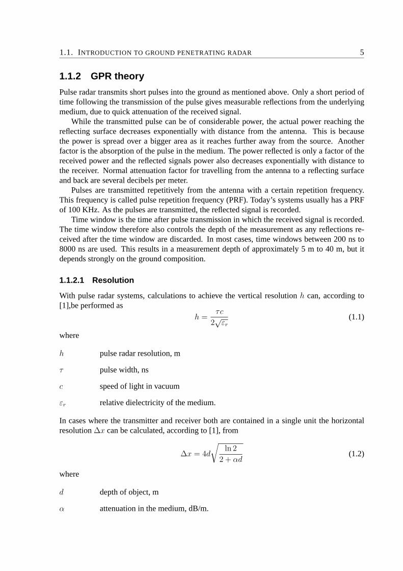
1.1.2.1 Resolution

With pulse radar systems, calculations to achieve the vertical resolutionh can, according to[1],be performed as

h =τc

2√

εr

(1.1)

where

h pulse radar resolution, m

τ pulse width, ns

c speed of light in vacuum

εr relative dielectricity of the medium.

In cases where the transmitter and receiver both are contained in a single unit the horizontalresolution∆x can be calculated, according to [1], from

∆x = 4d

√ln 2

2 + αd(1.2)

where

d depth of object, m

α attenuation in the medium, dB/m.

6 INTRODUCTION

Material Relative dielectricity Conductivity S/mClay (water-saturated) 8− 12 10−1 − 1Silt (water-saturated) 10 10−3 − 10−2

Sand (water-saturated) 30 10−4 − 10−2

Sand (dry) 4− 6 10−7 − 10−3

Air 1 0Fresh water 81 10−4 − 3 · 10−2

Seawater 81 4Fresh water ice 3.1− 4.3 10−3

Sea ice 4− 8 10−2 − 10−1

Snow 1.4 10−6 − 10−5

Concrete (dry) 6 1.2 · 10−3

Concrete (moistened for 20h) 10.9 7.1 · 10−3

Asphalt 2 (−6) 1.25 · 10−3

Table 1.1: Electrical properties for different materials.

The distances to the object can (according to [1]) be calculated using

s =twt · c2√

εr

(1.3)

where

twt signal travel time between the transmitting and receiving antenna via the reflectingobject

c speed of light in vacuum

εr relative dielectricity of the medium,

provided that the relative dielectricity of the medium is known. It is assumed that there is onlyone layer with dissimilar dielectricities between the antenna and the object. If that is not thecase, the distance can be calculated with respect of the different layer thicknesses calculatedfrom 1.3.

1.2 Capturing data from GPR

Capturing the data from a GPR survey is a most essential part of the measurement process, aslater performed post processing and interpretation usually is necessary to gain something fromthe survey. Previously analog recorders and plotters of different kinds where commonly usedto record and display scans from the survey. Today analog to digital conversion of the signal,followed by recording to a digital medium is the most commonly used method of data capture.

Digital capture opens up for new processing possibilities, but is not trivial to achieve be-cause of the high frequencies involved.

1.2. CAPTURING DATA FROM GPR 7T

ime

ns

1.

512 scans 1 scan

...

4.4.

1.

Figure 1.2: Time equivalent sampling.

1.2.1 Sampling theorem

Sampling of GPR signals needs to be done in very high speed. For an antenna with a centerfrequency of 70 MHz and a bandwidth of 70 MHz the signal will be within 35-105 MHz.According to Nyqvist’s sampling theorem the signal has to be sampled at a sampling frequencyabove 210 MHz .

Sampling Theorem [2]:If x(t) is a band-limited signal withX (jω) = 0 for |ω| > ωM . Thenx (t) is uniquely

determined by its samplesx (nT ) , n = 0, ±1, ±2, . . . , if

ωs > 2ωM , (1.4)

whereωs =

2π

T(1.5)

T sampling period

ωs sampling frequency

By generating a periodic impulse train where every impulse corresponds to a successful samplevalue we can reconstruct the signalx (t). To achieve an output signal that is exactly equal tox (t), the impulse train must be processed through an ideal low-pass filter with gainT andcutoff frequency,ωc, such asωM < ωc < ωs − ωM . If the sampling theorem is not fulfilledaliasing can occur where high frequency content takes on the identity of a lower frequency.

1.2.2 Time equivalent sampling

The fast analog to digital converters (ADC) needed for sampling GPR signals were until re-cently either very expensive or unavailable. Because of this a technique called time equivalent

8 INTRODUCTION

sampling is used to significantly reduce the sampling frequency required. It exploits the factthat if several scans are taken at about the same position, they will look almost the same. Witha pulse repetition frequency (PRF) of 100 KHz the antenna will only move a short distancebetween each scan, unless it is moving at a very high speed, making this sampling techniquework.

For every scan received, only one sample point is collected. The sample is first taken atthe beginning of the scan, and is delayed by some constant for each successive scan. To forma complete scan 200-2000 such data points, depending on the resolution required, are addedtogether as shown in figure 1.2.

With PRF as above, a sampling rate of only 100 KHz is needed, but the equivalent samplingrate can be several GHz. The downside of time equivalent sampling is that several scans arerequired to form a complete scan in digital form, slowing down the capturing process. Thisreduces the possibilities to stack scans (see 1.3.1).

1.2.3 Real-time sampling

The steady of evolution of ADC converters has in later years made high speed convertersavailable. Several manufacturers provide ADC chips with sampling rates up to 250 millionsamples per second (MSPS). Even higher speed chips are available from some manufacturers.Maxim has a 1600 MSPS analog to digital converter for example.

Using such a high speed converter allows for a complete digital conversion of a scan fromonly one source scan. Capturing the digital output from the converter presents another chal-lenge. With data rates of 250 MB/s or higher memories, data buses, processors and hard drivessets the limit. There are high speed memories available that can handle these data rates, butactually saving all the data to hard drives or other digital media is difficult and often unnec-essary. To actually take advantage of the higher speed of real-time sampling the data must beprocessed, first and foremost by stacking.

1.3 GPR Processing

The GPR signal usually goes through processing at some stage, the most common being dif-ferent kinds of filters during capture. More elaborate signal conditioning is sometimes done inpost processing. Another technique that can be used during capture though, is stacking.

1.3.1 Stacking

One of the biggest advantages of using real-time sampling instead of time equivalent samplingis the ability to stack scans rapidly. Stacking consists of taking the average of several scanscaptured at the same position1. The idea is that each individual scan will consist of the samesignal, except for noise. Averaging these scans will keep the signal while attenuating the noise,

1That is in the ideal case. Usually the antenna has moved a little between the individual scans but as long asthe movement is small the change in the scan is negligent.

1.4. PROJECT OBJECTIVE 9

improving the signal to noise ration (SNR) as given by

S

NGAIN(dB) = 10 log10 n (1.6)

where n is the number of scans averaged, according to [3]. The noise is assumed to be gaussian.Stacking is possible using time equivalent sampling as well. The problem is that time

equivalent sampling already requires several scans to create a complete digital scan, and tostack several such digital scans together requires (samples per scan)*(scans to stack) transmit-ted pulses. This quickly becomes too slow; with a PRF of 100KHz capturing enough data forstacking 64, 512-point, scans takes 0.3 seconds. Since the scans needs to be as similar as pos-sible during this time the radar must be moving very slowly. Under many circumstances thisis not possible2, and therefore stacking must be kept to a minimum. Using real-time samplinga complete digital scan is captured for every scan the antenna receives, and capturing 64 scansonly takes 0.64 ms as long as the capture system can keep up with the data rate.

Rapid stacking opens up for new possibilities with GPR. Because the signal level drops veryrapidly with the distance to the reflecting surface and will at longer distances be completelyhidden by noise, SNR is the limiting factor of the useful distance for GPR systems. With real-time sampling, stacking 1000 scans would improve SNR by 30 dB and still keep the systemas fast as the time equivalent sampling systems used today. An other way to improve SNR isto increase transmitter power thus increasing the signal level of the reflected signal. Becausethe SNR is increased by the same amount that the transmitter power is increased, a 30 dBimprovement in SNR would need a 30 dB increase in power. That means that 1000 times morepower is required. Constructing such a system would be very hard if even doable, makingstacking a more attractive choice for improving SNR.

An demonstration of the noise suppressing properties of stacking can be seen in figure 1.3.In this example noise was added to a sine wave. 1000 such waveforms were stacked togetherto remove the noise. The figure shows the waveforms of both a single waveform and thestacked waveform. To show how the noise is attenuated, the power spectrum density of the twowaveforms is also shown.

1.4 Project objective

The goal with this project was to examine the possibility to perform real-time sampling ofthe GPR signal with the high speed ADCs available today and the possibility to process thecaptured scans with a digital signal processor.

2for example when using an airborne system

10 INTRODUCTION

0 50 100 150 200−2

−1

0

1

2a

sample

ampl

itude

0 0.2 0.4 0.6 0.8 1−60

−40

−20

0

20

Frequency

Pow

er S

pect

rum

Mag

nitu

de (d

B)

b

0 50 100 150 200−1.5

−1

−0.5

0

0.5

1

1.5c

sample

ampl

itude

0 0.2 0.4 0.6 0.8 1−60

−40

−20

0

20

Frequency

Pow

er S

pect

rum

Mag

nitu

de (d

B)

d

Figure 1.3: Example of stacking. In (a) a sine wave with noise is shown, (b) is the correspondingspectral density. 1000 waveforms were stacked to produce (c), with corresponding spectral density in(d). The noise floor is lowered with about 30dB.

CHAPTER 2

Method and Results

Designing hardware that would fulfill our goals of real-time sampling and quick processingwas the first step in our project. Considerable time was consumed by finding an appropriateADC, DSP, and interfaces between the different parts. Next step, after building and testing thehardware, was to design the software for capturing, processing and displaying the GPR data. Acomplete real-time sampling GPR system with processing capabilities was then available forevaluation.

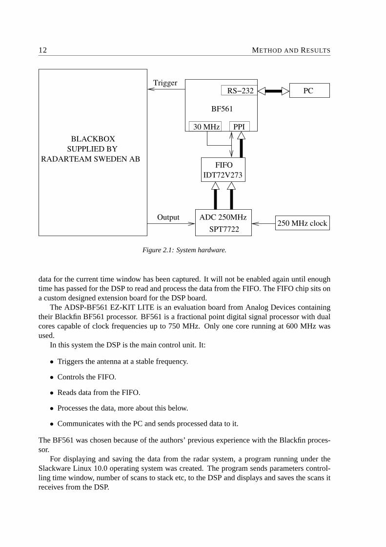
2.1 Hardware overview

An overview of the hardware used in this project can be seen in figure 2.1.For this project Radarteam Sweden AB lent a 40 MHz and 70 MHz antenna complete with

triggering and output system. To make the antenna transmit a pulse into the medium a shortpulse needs to be sent to the antennas trigger input. Keeping the operating conditions of theantenna stable requires that it is triggered at a stable frequency. Therefore pulses are sent at afrequency of 100 KHz to the antenna. The received signal is available on the output.

Real-time analog to digital conversion is done by a EB7722 ADC evaluation board kindlygiven to us by Fairchild Semiconductors. The board contains a SPT7722 ADC, a 8-bit ADCwith a maximum sampling frequency of 250 MHz, which it is also run at. The output from theconverter is demultiplexed to two ports, meaning that it delivers two 8-bit words in parallel ata frequency of 125 MHz, instead of one 8-bit word at 250 MHz which would have been thecase with a non-demultiplexed output. This makes the data from the ADC easier to captureas slower memories can be used, which was the main reason for choosing this ADC over anyother 250 MHz converter.

Data capture is performed by a first-in-first-out (FIFO) buffer chip from IDT especiallymade for bus matching, called IDT72V273. The chip has independently configurable inputand output bus widths, either 9- or 18-bits, and can handle frequencies up to 166 MHz. Hereit is used to capture the data from the ADC running at full speed, while letting the DSP readthe data at a lower data rate which it can handle. Of course, the lower data rate of the DSPinterface means that every waveform received from the antenna can not be captured. Onlywhen the DSP is ready, writing to the FIFO buffer is enabled. Writing is disabled when enough

11

12 METHOD AND RESULTS

250 MHz clock

PPI

BF561

30 MHz

PCRS−232

RADARTEAM SWEDEN AB

BLACKBOX

Trigger

Output

SUPPLIED BY

IDT72V273FIFO

ADC 250MHzSPT7722

Figure 2.1: System hardware.

data for the current time window has been captured. It will not be enabled again until enoughtime has passed for the DSP to read and process the data from the FIFO. The FIFO chip sits ona custom designed extension board for the DSP board.

The ADSP-BF561 EZ-KIT LITE is an evaluation board from Analog Devices containingtheir Blackfin BF561 processor. BF561 is a fractional point digital signal processor with dualcores capable of clock frequencies up to 750 MHz. Only one core running at 600 MHz wasused.

In this system the DSP is the main control unit. It:

• Triggers the antenna at a stable frequency.

• Controls the FIFO.

• Reads data from the FIFO.

• Processes the data, more about this below.

• Communicates with the PC and sends processed data to it.

The BF561 was chosen because of the authors’ previous experience with the Blackfin proces-sor.

For displaying and saving the data from the radar system, a program running under theSlackware Linux 10.0 operating system was created. The program sends parameters control-ling time window, number of scans to stack etc, to the DSP and displays and saves the scans itreceives from the DSP.

2.2. DSP SOFTWARE 13

2.2 DSP Software

In figure 2.2, a flow diagram of the workings of the DSP is shown. A walk trough of thedifferent steps follows.

2.2.1 Capture and stacking

The DSP outputs pulses to trigger the antenna at a frequency of 100 KHz independently ofanything else happening. When the program enters the capturing stage and thus is ready toactually receive and process data from the ADC, the capture needs to be synchronized with thetrigger pulse. If not, the data captured would most likely not contain the wanted waveform.

To get the capturing synchronized, the trigger pulse generates an interrupt at the sametime as the pulse is output. As this internally generated interrupt is received, writing to theFIFO chip is enabled. At the same time reading from the FIFO begins. After enough timefor capturing data for the current time window has passed, writing to the FIFO chip is againdisabled. Reading from the FIFO chip continues until it is finished.

This procedure gives data that is somewhat synchronized with the trigger pulse. Still thecapture timing may vary by several nanoseconds between different scans and sometimes up to100 nanoseconds. The reason for this timing variation depends on non-deterministic schedulingdelays of the Blackfin processor. In future hardware revisions, dedicated logic for controllingthe trigger and capture may be used to get stable timing.

After capture, the 8-bit data from the ADC is converted to 16-bit fractional values that isthe Blackfin’s native calculation unit. Doing all calculations in 16-bit resolution also meansless rounding errors than would be the case if 8-bit calculations were used.

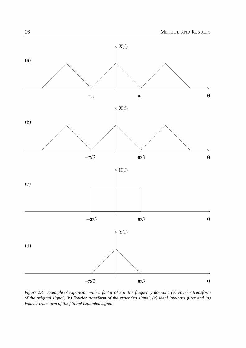
GPR data is usually oversampled several times with an equivalent sampling rate in the GHzrange. Sampling with a frequency,fs, of 250 MHz produces much fewer points than commonlyused in GPR and therefore expansion is used to try to recreate these missing points. Doing soalso allows for aligning of scans with higher precision.

Expansion is done by inserting zero values in between the actual data points. This newsignal is then low-pass filtered. The number of zeros inserted is equal to theN − 1, whereNis the expansion factor, and the cutoff frequency of the filter isfN

2NwherefN = fsN . After

expansion is done the signal contains the same data as if it had actually been sampled witha frequency offN . This is only true as long as the Nyquist condition was fulfilled beforesampling and if the low-pass filter is ideal. In this case a 10 fold expansion and the 39:th orderfinite impulse response (FIR) low-pass filter shown in figure 2.5 was used. An example ofexpansion and the effect it has in the time- and frequency domain can be seen in figure 2.3 and2.4. More on expansion can be found in [4].

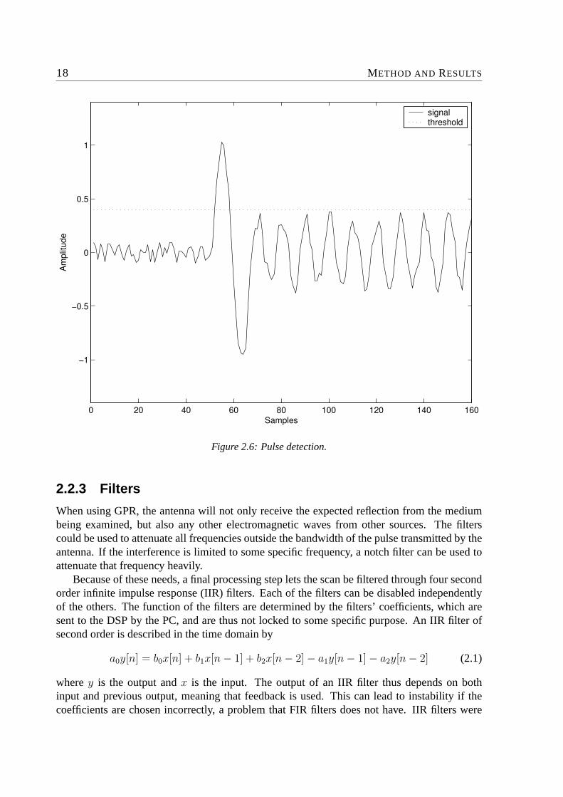
Since the scan alignment can vary as mentioned above, a technique for alignment is re-quired. In this case a falling edge detection to find a common edge that occurs in all scansis used. The detector finds the closest sample where the pulse goes from above to beneatha threshold value as shown in figure 2.6. This results in a fixed point in time relative to thetrigger, which is required for alignment.

The aligned scan is added to the accumulator, and the accumulator is then divided by 2 toprevent overflow. Doing stacking this way allows an arbitrary number of scans to be stackedwithout requiring more memory or risking overflow.


Figure 2.2: Flow diagram of the capture and processing of scans.


0 0.5 1 1.5 2 2.5 3 3.5 4 4.5 5−1

−0.5

0

0.5

1a

0 0.5 1 1.5 2 2.5 3 3.5 4 4.5 5−1.5

−1

−0.5

0

0.5

1

1.5b

Figure 2.3: Example of expansion. (a) 80 MHz sine wave sampled at 250MHz, (b) shows the same sinewave expanded with a factor of 10.

Only the processing needed for each single captured scan is done before stacking, lettingstacking be performed quickly. The captured scans used for stacking are therefore close in timeand also in position. After stacking is complete further processing can take place.

2.2.2 Time varying gain

As mentioned before, the received signal level from a reflecting surface will decrease veryrapidly with distance. This leads to two problems; one is that as the signal level gets lowerthe relative level of the quantization noise becomes higher and after a while the signal will beoutside the dynamic range of the ADC. This is especially true for 8-bit converters1, having atheoretical maximum dynamic range of only 48 dB. The second problem is that a reflectionsurface deep into the ground will give a weaker signal than an equivalent reflection surfacecloser to the antenna. It is easier to interpret the data if the two reflections show up with the

1which most high-speed converters are.


−π π

(d)

(c)

(b)

π/3−π/3

π/3−π/3

(a)

Y(f)

H(f)

X(f)

X(f)

θ

θ

θ

θπ/3−π/3

Figure 2.4: Example of expansion with a factor of 3 in the frequency domain: (a) Fourier transformof the original signal, (b) Fourier transform of the expanded signal, (c) ideal low-pass filter and (d)Fourier transform of the filtered expanded signal.


0 0.1 0.2 0.3 0.4 0.5 0.6 0.7 0.8 0.9−140

−120

−100

−80

−60

−40

−20

0

20

Normalized Frequency (×π rad/sample)

Mag

nitu

de (d

B)

Magnitude Response (dB)

Figure 2.5: Magnitude response for FIR-filter of order 39,ωstop = 0.095, ωpass = 0.11. ω is normalizedso thatω = 1 representsfs

2 .

same strength. To solve these two problems a time varying gain (TVG) must be applied.

Time varying gain is exactly what it sounds like: a gain of the signal varying with time.The gain increases as time from the pulse passes, counteracting the reduction in signal level. Inthis project a digital gain done by the Blackfin processor after the analog-to-digital conversionwas implemented. This only solves the second problem, and the signal level will go below thedynamic range of our ADC after about 10 or so meters, giving only noise after this distance.

To also solve the first problem the gain must be applied on the analog signal before con-version. This is not a trivial problem as the bandwidth of the amplifier must cover the wholesignal spectrum and the gain must increase very quickly. How to build such an amplifier isoutside the scope of this report2.

2and also outside the authors’ area of expertise


0 20 40 60 80 100 120 140 160

−1

−0.5

0

0.5

1

Samples

Am

plitu

de

signalthreshold

Figure 2.6: Pulse detection.

2.2.3 Filters

When using GPR, the antenna will not only receive the expected reflection from the mediumbeing examined, but also any other electromagnetic waves from other sources. The filterscould be used to attenuate all frequencies outside the bandwidth of the pulse transmitted by theantenna. If the interference is limited to some specific frequency, a notch filter can be used toattenuate that frequency heavily.

Because of these needs, a final processing step lets the scan be filtered through four secondorder infinite impulse response (IIR) filters. Each of the filters can be disabled independentlyof the others. The function of the filters are determined by the filters’ coefficients, which aresent to the DSP by the PC, and are thus not locked to some specific purpose. An IIR filter ofsecond order is described in the time domain by

a0y[n] = b0x[n] + b1x[n− 1] + b2x[n− 2]− a1y[n− 1]− a2y[n− 2] (2.1)

wherey is the output andx is the input. The output of an IIR filter thus depends on bothinput and previous output, meaning that feedback is used. This can lead to instability if thecoefficients are chosen incorrectly, a problem that FIR filters does not have. IIR filters were

2.3. PC SOFTWARE 19

low-pass (second-order) withK = tan(πfc/fs)

b0 = K2

1+√

2K+K2 b1 = 2K2

1+√

2K+K2 b2 = K2

1+√

2K+K2 a1 = 2(K2−1)

1+√

2K+K2 a2 = 1−√

2K+K2

1+√

2K+K2

high-pass (second-order) withK = tan(πfc/fs)

b0 = 11+√

2K+K2 b1 = −21+√

2K+K2 b2 = 11+√

2K+K2 a1 = 2(K2−1)

1+√

2K+K2 a2 = 1−√

2K+K2

1+√

2K+K2

Table 2.1: Filter coefficients for low-pass and high-pass filters [5]. The coefficients are normalized sothata0 = 1.

used because of the computational savings they give over FIR filters, and also because of theirrelatively easy parameterisation. The above difference equation gives the following equationin the frequency domain:

H(ejΩ) =b0 + b1e

−jΩ + b2e−j2Ω

a0 + a1e−jΩ + a2e−j2Ω(2.2)

whereΩ = 2π ffs

. Formulas for calculating the coefficients for both high-pass and low-passfilter with a given cutoff frequency are given in table 2.1. The formulas are used by the PCsoftware to calculate coefficients for sending to the DSP.

In this system, the antenna bandwidth is close to the Nyquist limit of the analog to digitalconversion rate used. Therefore the filters’ application is somewhat limited. They were mostlyadded to examine the possibility of digital filtering and the processing time required.

2.2.4 Communication with PC

When the scan has passed through all the processing steps, it is transformed back to 8-bit valuesand transmitted to the PC through a RS-232 interface. The RS-232 connection uses a baud rateof 230400 and is the limiting factor for the system’s speed. For example, the connection canonly send about 14 scans per second, each 512 nanosecond long, even though the DSP cancapture and process them much faster.

To keep the PC and DSP communication synchronized a simple protocol inspired by PPPwas designed. It handles framing of data and does checksum calculations. Without such aprotocol missing a byte in the data stream would have been fatal, since the data would havebeen misinterpreted and there would have been no way to get back in sync. The protocol addsa data overhead, although small, making the transmission slower.

2.3 PC Software

The PC software is the user interface of the radar system. It lets the user set parameters such astime window, number of scans to stack, time varying gain, filters, and various parameters usedfor debugging. These parameters are then pushed to the DSP that does the actual capture andprocessing.

When a scan is received the scan is plotted both in a oscilloscope view and in a intensityplot view, the latter also containing a history of the latest scans. At the same time the scan is


Figure 2.7: PC interface.

saved on disk, allowing for later inspection and further processing. Figure 2.7 shows a screenshot of the interface.

2.4 Results

The speed of the system was examined by measuring control signals with an oscilloscope. Forevery scan captured the write control for the FIFO chip is toggled on and off. Looking attime elapsed between each such toggle gives an accurate measurement for the time needed tocapture, interpolate and stack one scan. Of course that time varies with the amount of datacaptured, ie the time window. The time needed for applying TVG and filtering was measuredin the same way. The result are shown in table 2.2.

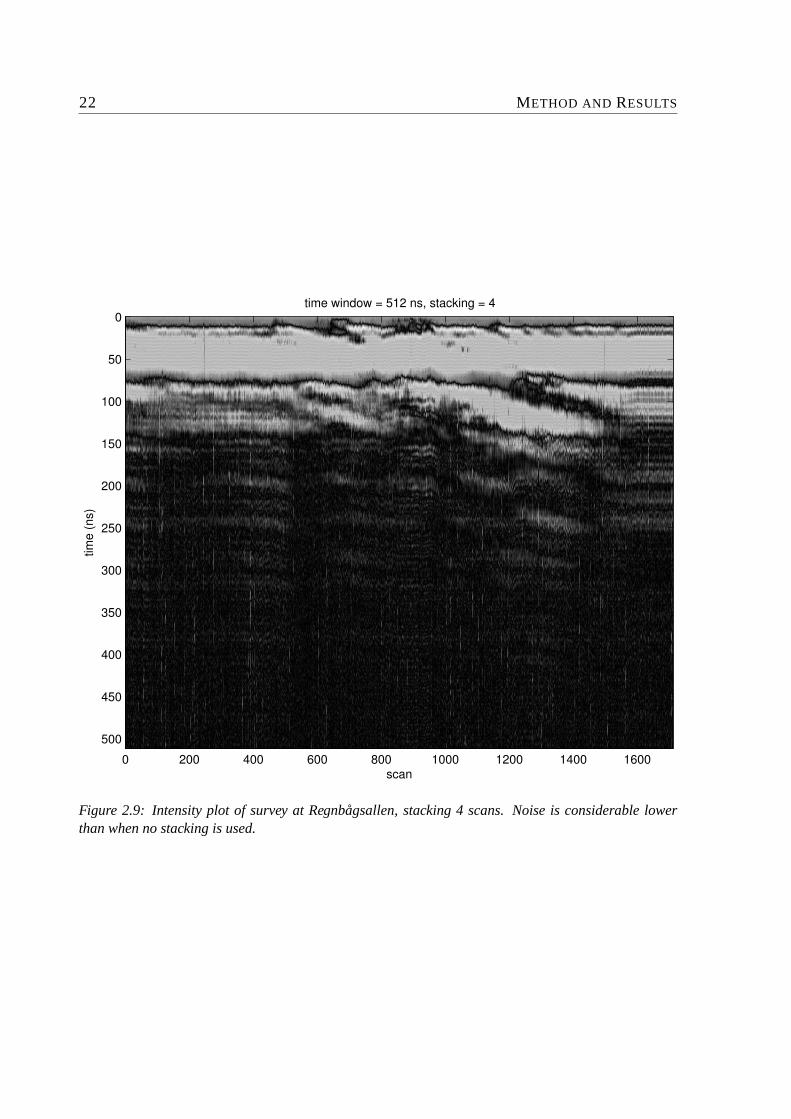
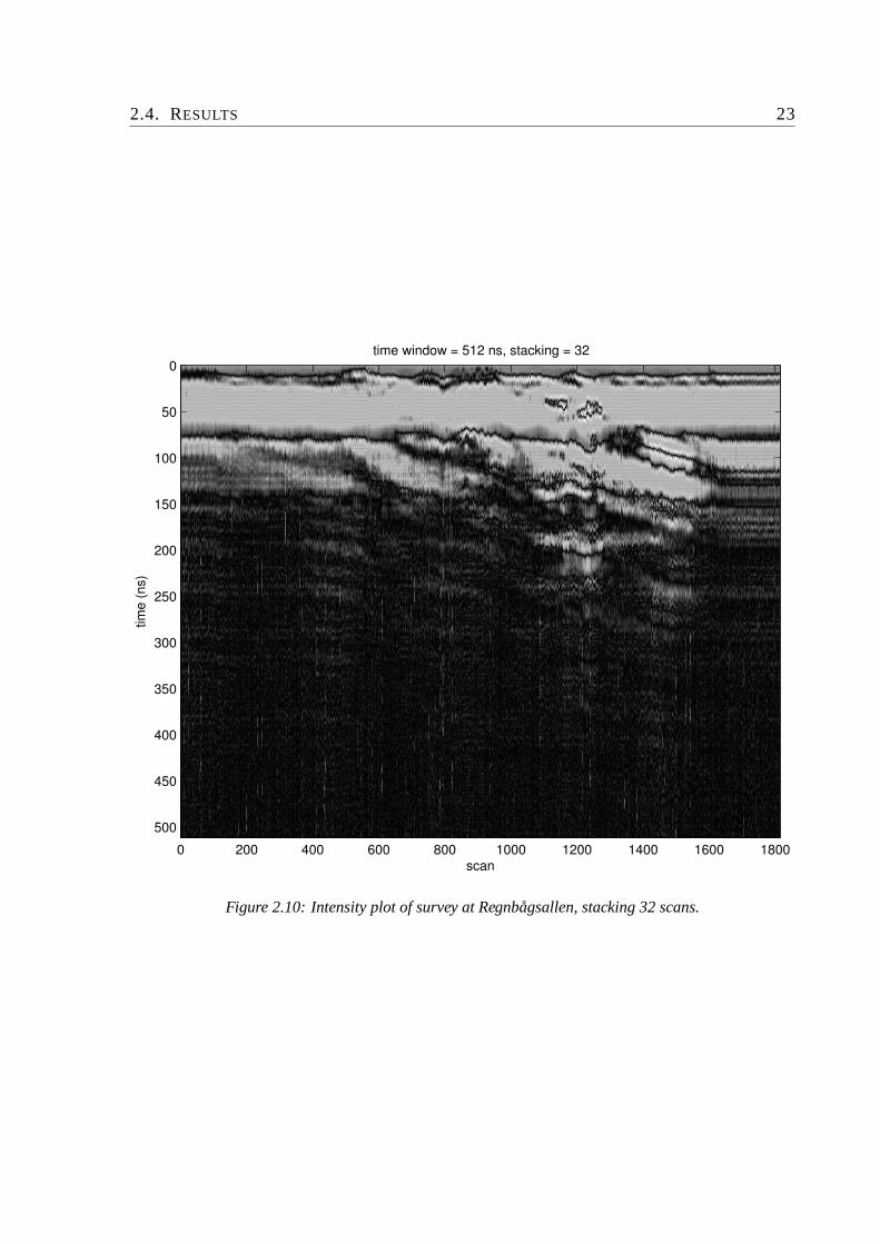
To get a picture of how the system worked and the effects of stacking and the other pro-cessing steps on a real field survey, a sample survey was performed at Regnbagsallen at LuleaUniversity of Technology. Different stacking, and other, settings were used. Intensity plots ofthe results are shown in figure 2.8, 2.9 and 2.10. The first 100 ns are the results of residualsfrom the antenna and not actual reflections. White vertical lines are scattered over the pictures,the source of these are unknown, but might be some interference picked up by the antenna. Go-ing from no stacking to stacking 4 scans shows a noticeable reduction in noise. The differencebetween stacking 4 and 32 scans is harder to see.

2.4. RESULTS 21

Samples Time window (ns) Stacking TVG Filtering Total520 208 2941 29410 14880 1801280 512 2325 11960 6097 1402520 1008 1754 6060 3105 1045000 2000 1136 2762 1302 6612520 5008 476 1068 476 27

Table 2.2: Number of scans per second that can be processed during different parts of the data process-ing. The total column shown the number of completely processed scans that the system could outputwhen using stacking of 16.

scan

time

(ns)

time window = 512 ns, stacking = 1

0 500 1000 1500

0

50

100

150

200

250

300

350

400

450

500

Figure 2.8: Intensity plot of survey at Regnbagsallen, no stacking.


scan

time

(ns)


0 200 400 600 800 1000 1200 1400 1600

0

50

100

150

200

250

300

350

400

450

500

Figure 2.9: Intensity plot of survey at Regnbagsallen, stacking 4 scans. Noise is considerable lowerthan when no stacking is used.

2.4. RESULTS 23

scan

time

(ns)


0 200 400 600 800 1000 1200 1400 1600 1800

0

50

100

150

200

250

300

350

400

450

500

Figure 2.10: Intensity plot of survey at Regnbagsallen, stacking 32 scans.


CHAPTER 3

Conclusions

We have shown that it is possible to perform real-time sampling of GPR with commonly avail-able equipment. The processing performance of the system is adequate for many needs, andcould be further improved by code optimization and use of both processor cores.

Some blocks for achieving overall high performance are still missing. For example theanalog time varying gain amplifier before the ADC needed to keep the signal level within theconverters dynamic range. Constructing such an amplifier is outside our expertise, and proba-bly hard even for someone with the appropriate competence. However, it is not impossible andhas already been done [3].

A more trivial problem is improving the transfer speed from the DSP to the PC. Because thiswas a prototype system, we used the outputs available on the DSP board for communication,instead of adding communication circuitry to the extension board. Using the RS-232 interfacewas good enough for our needs, but for a real GPR system a higher transfer speed is necessary.When building the custom PCB that a production type system would most probably use, afaster interface can be added.

The varying delay from when the antenna is triggered till when capture of the scan beginsgives us a little jitter even after aligning the scans with pulse detection. To get stable timing,hardware based logic could be used to start the capture. For even better alignment, the ADCsample clock and trigger pulse clock should be synchronized, for example by using the sameclock source for both.

With a sample rate of 250 MHz, even a 70 MHz antenna is on the limit of what this systemcan handle without aliasing problems. As mentioned, faster ADCs are available, but to capturethe data from such a converter a more complex capturing system than what we used is needed.

The biggest challenge for us during the project, was to design the hardware and especiallythe FIFO extension board. Neither of us had any serious previous experience of electronicsdesign, so this was something we had to learn during the project. However, we learnt a lot, andthis proved to be maybe the most rewarding part of our work.

Implementation of the software was relatively straightforward. We must mention the devel-opment environment for the DSP card, Visual DSP++, though. This program was the sourceof much frustration and delay, as it would often crash and later refuse to start. Half a day couldbe spent to get it working again. It is our hope that Analog Devices will focus on fixing bugs

25

26 CONCLUSIONS

for the next versions and let features wait.

APPENDIX A

Abbreviations

ADC Analog to digital converter.

DSP Digital signal processor.

FIFO First-in-first-out.

FIR Finite impulse response.

GPR Ground penetrating radar.

IIR Infinite impulse response.

MSPS Million samples per second.

PRF Pulse repetition frequency.

SNR Signal to noise ratio.

TVG Time varying gain.

27

28 APPENDIX A

REFERENCES

[1] P. Maijala, Ground Penetrating Radar and Related Processing Techniques. PhD thesis,University of Oulu, Department of Geophysics, 1994.

[2] A. V. Oppenheim and A. S. Willsky,Signals & Systems. Upper Saddle River, New Jersey:Prentice-Hall, second ed., 1997.

[3] D. Wright, J. Bradley, and T. Grover, “Data aquisition systems for ground penetratingradar with example application from the air, surface, and boreholes,”Proceedings of theFifth Internatilnal Conference on Ground Penetrating Radar, vol. 3 of 3, pp. 1075–1089,Jun 1994.

[4] B. Porat,A Course in Digital Signal Processing. New York: Wiley & Sons, 1997.

[5] U. Zolzer, ed.,DAFX: Digital Audio Effects. Chichester: Wiley, 2002.

29

Documents

Real-time sampling of Ground Penetrating Radar and Related