Real-time rendering of large terrains using algorithms for continuous level of detail

(HS-IDA-EA-02-103)

Michael Andersson (a98mican@ida.his.se)

Department of Computer Science University of Skövde, Box 408 S-54128 Skövde, SWEDEN

Final Year Project in Computer Science, spring 2002. Supervisor: Mikael Thieme

[Real-time rendering of large terrains using algorithms for continuous level of detail]

Submitted by Michael Andersson to Högskolan Skövde as a dissertation for the degree of B.Sc., in the Department of Computer Science.

[date]

I certify that all material in this dissertation, which is not my own work has been identified and that no material is included for which a degree has previously been conferred on me.

Signed: _______________________________________________

Real-time rendering of large terrains using algorithms for continuous level of detail

Michael Andersson (a98mican@ida.his.se)

Summary Three-dimensional computer graphics enjoys a wide range of applications of which games and movies are only few examples. By incorporating three-dimensional computer graphics in to a simulator the simulator is able to provide the operator with visual feedback during a simulation. Simulators come in many different flavors where flight and radar simulators are two types in which three-dimensional rendering of large terrains constitutes a central component.

Ericsson Microwave Systems (EMW) in Skövde is searching for an algorithm that (a) can handle terrain data that is larger than physical memory and (b) has an adjustable error metric that can be used to reduce terrain detail level if an increase in load on other critical parts of the system is observed. The aim of this paper is to identify and evaluate existing algorithms for terrain rendering in order to find those that meet EMW: s requirements. The objectives are to (i) perform a literature survey over existing algorithms, (ii) implement these algorithms and (iii) develop a test environment in which these algorithms can be evaluated form a performance perspective.

The literature survey revealed that the algorithm developed by Lindstrom and Pascucci (2001) is the only algorithm of those examined that succeeded to fulfill the requirements without modifications or extra software. This algorithm uses memory-mapped files to be able to handle terrain data larger that physical memory and focuses on how terrain data should be laid out on disk in order to minimize the number of page faults. Testing of this algorithm on specified test architecture show that the error metric used could be adjusted to effectively control the terrains level of detail leading to a substantial increase in performance. The results also reveal the need for both view frustum culling as well a level of detail algorithm to achieve fast display rates of large terrains. Further the results also show the importance of how terrain data is laid out on disk especially when physical memory is limited.

Keywords: real-time, rendering, terrain, algorithm

I

Table of contents 1 Introduction ...................................................................................1

2 Background ....................................................................................5

2.1 The three-dimensional graphics pipeline .......................................................5

2.2 View frustum culling ....................................................................................9

2.3 Level of detail...............................................................................................9

2.4 Algorithms..................................................................................................11

2.4.1 Real-time, continuous level of detail rendering of height fields ............................... 11

2.4.2 Real-time optimally adapting meshes ..................................................................... 15

2.4.3 Real-Time generation of continuous levels of detail for height fields ...................... 18

2.4.4 A fast algorithm for large scale terrain walkthrough ............................................... 20

2.4.5 Visualization of large terrains made easy................................................................ 21

3 Problem ........................................................................................ 25

3.1 Problem definition ......................................................................................25

3.2 Delimitation................................................................................................25

3.3 Expected result ...........................................................................................25

4 Method.......................................................................................... 26

4.1 Test architecture .........................................................................................26

4.2 Test cases ...................................................................................................26

4.2.1 Terrain .................................................................................................................. 26

4.2.2 Path....................................................................................................................... 26

4.2.3 Operation .............................................................................................................. 27

4.2.4 Physical memory ................................................................................................... 27

5 Implementation ............................................................................ 28

5.1 Algorithm selection ....................................................................................28

5.2 Memory mapped files .................................................................................28

5.3 Additional test cases ...................................................................................29

5.3.1 File layout ............................................................................................................. 29

5.3.2 Adjustable error metric .......................................................................................... 29

5.3.3 Terrain revisited..................................................................................................... 29

5.3.4 Physical memory revisited ..................................................................................... 29

6 Results and analysis ..................................................................... 30

7 Discussion ..................................................................................... 34

8 Conclusion .................................................................................... 35

9 Future work.................................................................................. 36

II

10 References..................................................................................... 37

11 Appendix A................................................................................... 38

12 Appendix B................................................................................... 39

1

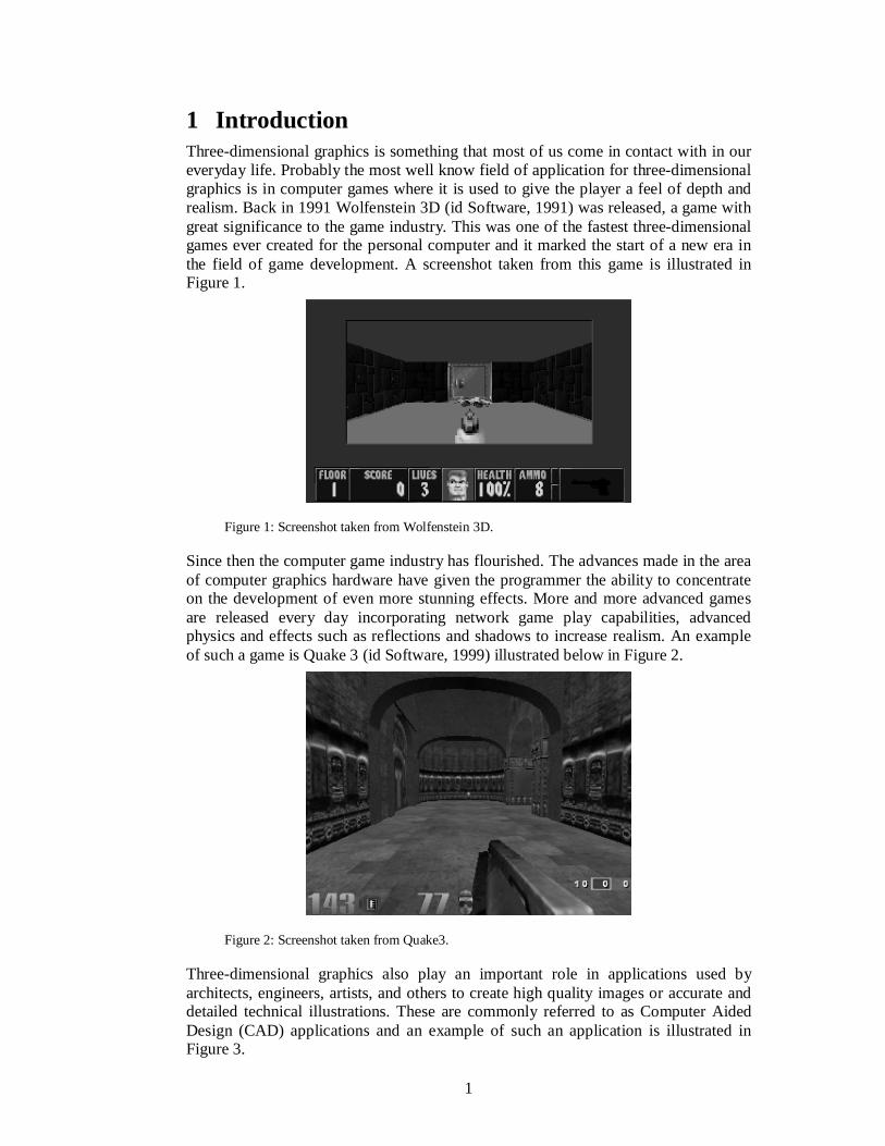
1 Introduction Three-dimensional graphics is something that most of us come in contact with in our everyday life. Probably the most well know field of application for three-dimensional graphics is in computer games where it is used to give the player a feel of depth and realism. Back in 1991 Wolfenstein 3D (id Software, 1991) was released, a game with great significance to the game industry. This was one of the fastest three-dimensional games ever created for the personal computer and it marked the start of a new era in the field of game development. A screenshot taken from this game is illustrated in Figure 1.

Figure 1: Screenshot taken from Wolfenstein 3D.

Since then the computer game industry has flourished. The advances made in the area of computer graphics hardware have given the programmer the ability to concentrate on the development of even more stunning effects. More and more advanced games are released every day incorporating network game play capabilities, advanced physics and effects such as reflections and shadows to increase realism. An example of such a game is Quake 3 (id Software, 1999) illustrated below in Figure 2.

Figure 2: Screenshot taken from Quake3.

Three-dimensional graphics also play an important role in applications used by architects, engineers, artists, and others to create high quality images or accurate and detailed technical illustrations. These are commonly referred to as Computer Aided Design (CAD) applications and an example of such an application is illustrated in Figure 3.

2

Figure 3: Illustration of a model created with Design CAD 3D Max (Upperspace Coorp, 2001)

Those areas described so far are not its only range of applications. Three-dimensional graphics also play an important role in different kinds of military simulators such as radar and flight simulators (see Figure 4). In both these types of simulators three-dimensional graphics is used to visualize the environment in which the simulation takes place. One way to represent the environment is by using sampled terrain data, which in conjunction with three-dimensional graphics can be used to render an image of surroundings.

Figure 4: Screenshot from the Terra3D terrain engine (Wortham, 2002).

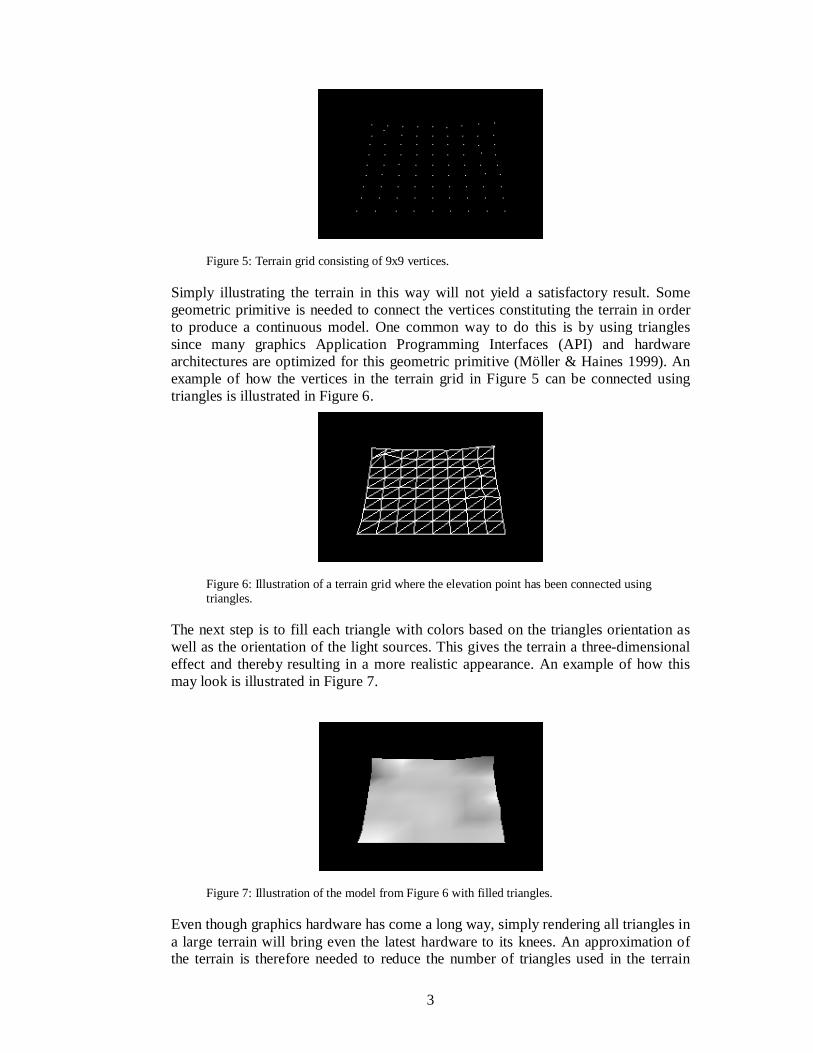
The three-dimensional terrain data used by these simulators can be represented in several different ways. One common way is to use a rectangular grid of vertices (elevation points) often referred to as a height field. An example of such a grid is illustrated in Figure 5.

3

Figure 5: Terrain grid consisting of 9x9 vertices.

Simply illustrating the terrain in this way will not yield a satisfactory result. Some geometric primitive is needed to connect the vertices constituting the terrain in order to produce a continuous model. One common way to do this is by using triangles since many graphics Application Programming Interfaces (API) and hardware architectures are optimized for this geometric primitive (Möller & Haines 1999). An example of how the vertices in the terrain grid in Figure 5 can be connected using triangles is illustrated in Figure 6.

Figure 6: Illustration of a terrain grid where the elevation point has been connected using triangles.

The next step is to fill each triangle with colors based on the triangles orientation as well as the orientation of the light sources. This gives the terrain a three-dimensional effect and thereby resulting in a more realistic appearance. An example of how this may look is illustrated in Figure 7.

Figure 7: Illustration of the model from Figure 6 with filled triangles.

Even though graphics hardware has come a long way, simply rendering all triangles in a large terrain will bring even the latest hardware to its knees. An approximation of the terrain is therefore needed to reduce the number of triangles used in the terrain

4

without compromising visual quality (Röttger, et al. 1998). These approximation algorithms are refereed to as level of detail (LOD) algorithms. Such algorithms perform on-the-fly approximation of the terrain where regions closer to the viewer as well as regions with higher roughness is approximated using more triangles compared to regions that are farther away or more flat. An example of how this may look is illustrated in Figure 8.

Figure 8: Example of a terrain with decreased detail. The viewer is presumed to be located at the lower right corner.

Ericsson Microwave Systems (EMW) in Skövde develops simulators that with high accuracy can reproduce radar functionality. EMW is looking for a terrain rendering algorithms that meets the following requirements:

1. The algorithm should be able to handle terrain data that is larger than main memory of a single personal computer.

2. The algorithm should be able to adjust the level of detail of the terrain if the load on other relatively more critical parts of the system exceeds some threshold.

The aim of this paper is to identify and evaluate existing algorithms that conform to EMW: s requirements. The objectives derived form this aim is to (i) perform a litterateur survey over existing algorithms, (ii) implement the algorithms that meets EMW: s requirements and (iii) develop a test environment in which these algorithms can be evaluated from a performance perspective.

5

2 Background This section begins with a description of the three-dimensional graphics pipeline of which knowledge is important in order to understand the concepts related to three-dimensional computer graphics as well as terrain rendering. This is followed by a description of view-frustum culling in Section 2.2, a technique used to further enhance performance by preventing non-visible geometry from being sent through the pipeline. In Section 2.3 the concept behind level of detail algorithms will be discussed. Such algorithms exploit the fact that parts of the terrain that are further away from the viewer and/or more flat can be approximated using fewer triangles, without compromising visual quality, compared to those regions that are closer and/or more rough. Last, in Section 2.4 different continuous level of detail algorithms for terrain rendering will be described in detail.

2.1 The three-dimensional graphics pipeline

The purpose of the three-dimensional graphics pipeline is to; given a virtual camera, three-dimensional object, light sources, lighting models, textures and more render a two-dimensional image (Möller & Haines 1999). Knowledge of the three-dimensional graphics pipeline is fundamental in order to be able to understand the concepts of three-dimensional terrain rendering. The purpose of this section is therefore to discuss the pipeline and explain its different stages.

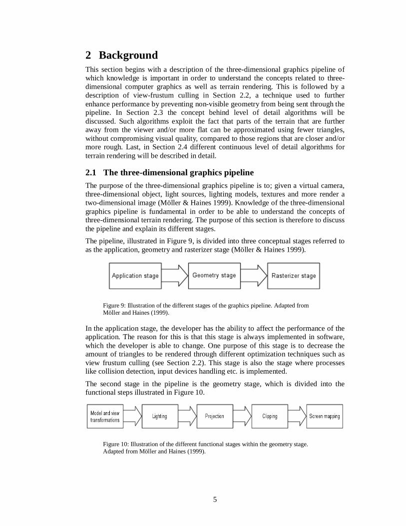
The pipeline, illustrated in Figure 9, is divided into three conceptual stages referred to as the application, geometry and rasterizer stage (Möller & Haines 1999).

Figure 9: Illustration of the different stages of the graphics pipeline. Adapted from Möller and Haines (1999).

In the application stage, the developer has the ability to affect the performance of the application. The reason for this is that this stage is always implemented in software, which the developer is able to change. One purpose of this stage is to decrease the amount of triangles to be rendered through different optimization techniques such as view frustum culling (see Section 2.2). This stage is also the stage where processes like collision detection, input devices handling etc. is implemented.

The second stage in the pipeline is the geometry stage, which is divided into the functional steps illustrated in Figure 10.

Figure 10: Illustration of the different functional stages within the geometry stage. Adapted from Möller and Haines (1999).

6

The modeling and rendering of a cube will be used to explain these different stages. First, the cube is created in its own local coordinate system also known as model space as illustrated in Figure 11.

Figure 11: An illustration of the cube located in model space. The viewer is presumed to be looking down the negative y-axis. Adapted from Möller and Haines (1999).

The cube is associated with a set of model transformations, which affects the cube position and orientation as illustrated in Figure 12, i.e. places the cube at the appropriate position and orientation in the virtual world.

Figure 12: Illustration of the cube position, orientation and shape after the model transformations (a) rotation, (b) scaling, (c) translation, (d) all together. Adapted from Möller and Haines (1999).

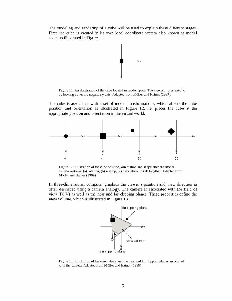
In three-dimensional computer graphics the viewer’s position and view direction is often described using a camera analogy. The camera is associated with the field of view (FOV) as well as the near and far clipping planes. These properties define the view volume, which is illustrated in Figure 13.

Figure 13: Illustration of the orientation, and the near and far clipping planes associated with the camera. Adapted from Möller and Haines (1999).

7

The goal is to render only those models that are within or intersect the camera’s view volume. Therefore, in order to facilitate projection and clipping, a view transformation is applied to the camera as well as the cube as illustrated in Figure 14.

Figure 14: The position and orientation of the camera and cube after view transformation. The cameras view direction is now aligned with the negative z-axis. Adapted from Möller and Haines (1999).

After the view transformations the camera and the cube is said to reside in camera or eye space in which projection and clipping operations are made simpler and faster (Möller & Haines 1999).

The second functional step is the lighting step. The cube will not have a realistic feel unless one or more light sources are added and therefore equations that approximate real world lights are used to compute the color at each vertex of the cube. This computation is performed using the properties and locations of the light sources as well as the position, normal and material properties of the vertex. Later on when the cube is to be rendered to the screen the colors at each vertex are interpolated over the cubes surfaces, a technique know as the Gouraud shading (Möller & Haines, 1999).

The next step is the projection step. In terrain rendering the most common type of projection is called perspective projection in which the view volume is shaped like a so-called frustum, a truncated pyramid with rectangular base. An illustration of the frustum used in perspective projection is given in Figure 15.

Figure 15: Illustration of the view frustum used in perspective projection. As the figure illustrates the view frustum is shaped like a pyramid with its top cut off.

An important characteristic of this type of projection is that the cube will become smaller as the distance between it and the camera increases. This result is exploited by

8

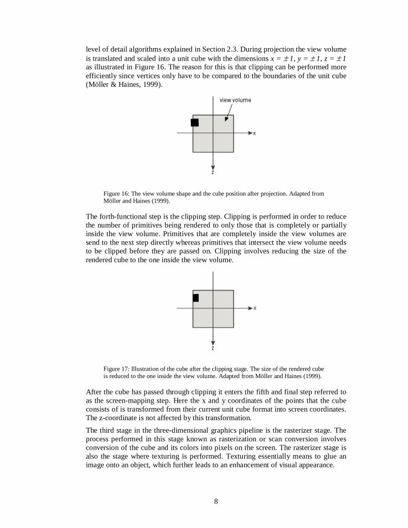
level of detail algorithms explained in Section 2.3. During projection the view volume is translated and scaled into a unit cube with the dimensions x = ± 1, y = ± 1, z = ± 1 as illustrated in Figure 16. The reason for this is that clipping can be performed more efficiently since vertices only have to be compared to the boundaries of the unit cube (Möller & Haines, 1999).

Figure 16: The view volume shape and the cube position after projection. Adapted from Möller and Haines (1999).

The forth-functional step is the clipping step. Clipping is performed in order to reduce the number of primitives being rendered to only those that is completely or partially inside the view volume. Primitives that are completely inside the view volumes are send to the next step directly whereas primitives that intersect the view volume needs to be clipped before they are passed on. Clipping involves reducing the size of the rendered cube to the one inside the view volume.

Figure 17: Illustration of the cube after the clipping stage. The size of the rendered cube is reduced to the one inside the view volume. Adapted from Möller and Haines (1999).

After the cube has passed through clipping it enters the fifth and final step referred to as the screen-mapping step. Here the x and y coordinates of the points that the cube consists of is transformed from their current unit cube format into screen coordinates. The z-coordinate is not affected by this transformation.

The third stage in the three-dimensional graphics pipeline is the rasterizer stage. The process performed in this stage known as rasterization or scan conversion involves conversion of the cube and its colors into pixels on the screen. The rasterizer stage is also the stage where texturing is performed. Texturing essentially means to glue an image onto an object, which further leads to an enhancement of visual appearance.

9

2.2 View frustum culling

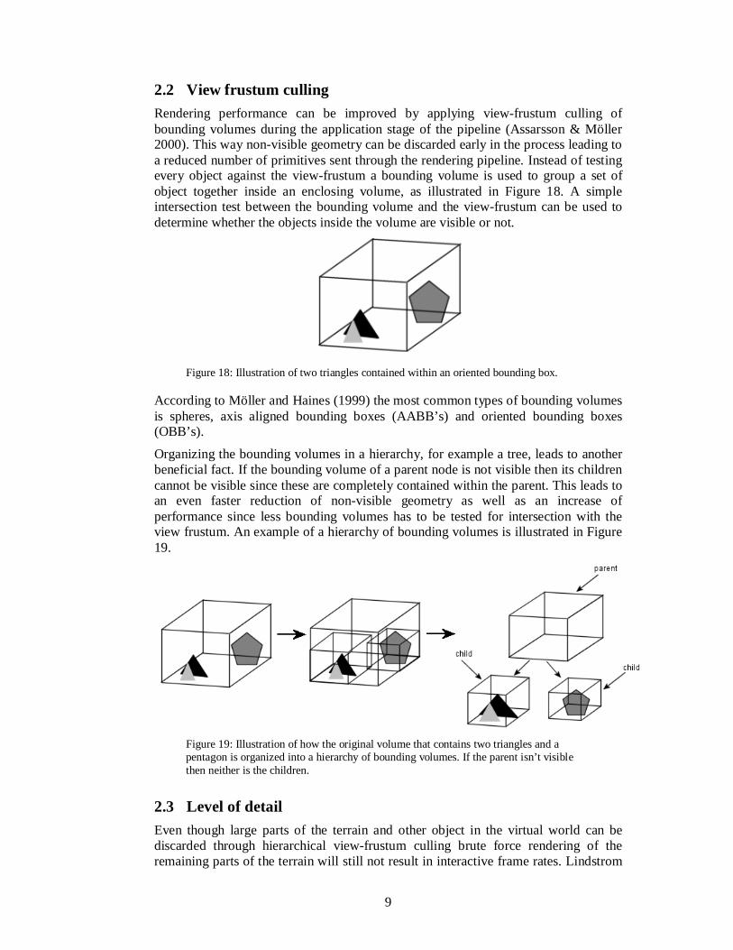
Rendering performance can be improved by applying view-frustum culling of bounding volumes during the application stage of the pipeline (Assarsson & Möller 2000). This way non-visible geometry can be discarded early in the process leading to a reduced number of primitives sent through the rendering pipeline. Instead of testing every object against the view-frustum a bounding volume is used to group a set of object together inside an enclosing volume, as illustrated in Figure 18. A simple intersection test between the bounding volume and the view-frustum can be used to determine whether the objects inside the volume are visible or not.

Figure 18: Illustration of two triangles contained within an oriented bounding box.

According to Möller and Haines (1999) the most common types of bounding volumes is spheres, axis aligned bounding boxes (AABB’s) and oriented bounding boxes (OBB’s).

Organizing the bounding volumes in a hierarchy, for example a tree, leads to another beneficial fact. If the bounding volume of a parent node is not visible then its children cannot be visible since these are completely contained within the parent. This leads to an even faster reduction of non-visible geometry as well as an increase of performance since less bounding volumes has to be tested for intersection with the view frustum. An example of a hierarchy of bounding volumes is illustrated in Figure 19.

Figure 19: Illustration of how the original volume that contains two triangles and a pentagon is organized into a hierarchy of bounding volumes. If the parent isn’t visible then neither is the children.

2.3 Level of detail

Even though large parts of the terrain and other object in the virtual world can be discarded through hierarchical view-frustum culling brute force rendering of the remaining parts of the terrain will still not result in interactive frame rates. Lindstrom

10

and Pascucci (2001) argue that it is essential to perform on-the-fly simplification of a high-resolution mesh in order to accommodate fast display rates. This simplification process is commonly refereed to level of detail (LOD). LOD exploits the fact that when the distance from a model to the viewpoint increases the model can be approximated with a simpler version, without compromising visual quality. The reason that visual quality is not compromised is because of the main characteristic of perspective projection, explained in Section 2.1, which states that an object will be smaller as it gets further way from the viewpoint thus covering a less area of pixels.

The simplest type of LOD is discrete LOD (DLOD) (Möller & Haines 1999), which uses different models of the same object where each model is an approximation of the original object using fewer primitives. Switching between detail levels is done when the distance from the viewpoint to the object is greater or equal to that levels associated threshold value. Using this type of LOD a switch during rendering often produces a noticeable and not visually appealing “popping effect” when the level of detail suddenly is decreased (Ederly 2001). An example of the work of a DLOD algorithm is illustrated in Figure 20.

Figure 20: Illustration of three different discrete levels of detail. As the viewer moves further away form or closer to the terrain a switch between these levels of detail is conducted.

When working with terrain rendering DLOD can be applied to small parts of the terrain, know as blocks instead of the entire terrain. An example of a terrain rendered with block DLOD is illustrated in Figure 8.

Another type of LOD is continuous LOD (CLOD), which is based on dynamic triangulation of the model where a small amount of triangles are changed at a time (Röttger, et al. 1998; Ederly 2001). The advantage of using CLOD instead of DLOD is that, since CLOD only removes a small number of triangles, the popping effect becomes less noticeable. The reduced level of detail produced by a CLOD algorithm is illustrated below in Figure 21.

Figure 21: Illustration of the work performed by a continuous level of detail algorithm. As the viewer moves further away from lower right corner of the terrain the detail level is slowly reduced.

A problem that often occurs when using the block DLOD and CLOD methods in terrain rendering is the occurrence of cracks between adjacent terrain blocks with

11

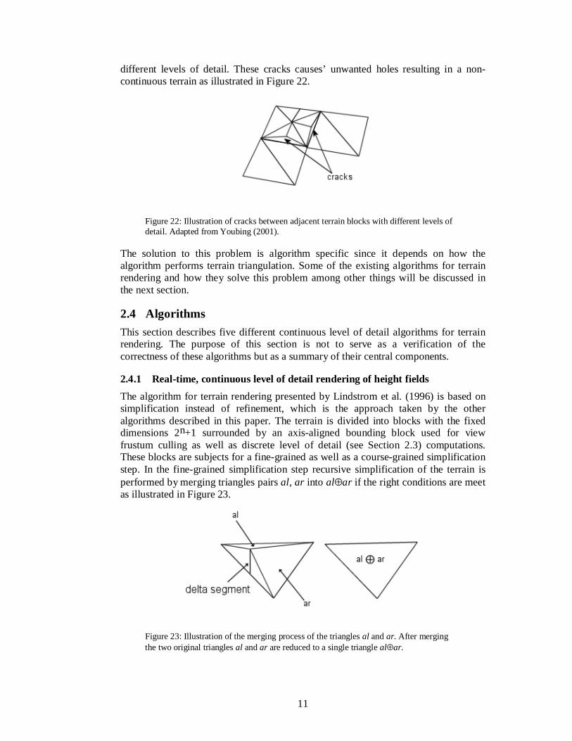
different levels of detail. These cracks causes’ unwanted holes resulting in a non-continuous terrain as illustrated in Figure 22.

Figure 22: Illustration of cracks between adjacent terrain blocks with different levels of detail. Adapted from Youbing (2001).

The solution to this problem is algorithm specific since it depends on how the algorithm performs terrain triangulation. Some of the existing algorithms for terrain rendering and how they solve this problem among other things will be discussed in the next section.

2.4 Algorithms

This section describes five different continuous level of detail algorithms for terrain rendering. The purpose of this section is not to serve as a verification of the correctness of these algorithms but as a summary of their central components.

2.4.1 Real-time, continuous level of detail rendering of height fields

The algorithm for terrain rendering presented by Lindstrom et al. (1996) is based on simplification instead of refinement, which is the approach taken by the other algorithms described in this paper. The terrain is divided into blocks with the fixed dimensions 2n+1 surrounded by an axis-aligned bounding block used for view frustum culling as well as discrete level of detail (see Section 2.3) computations. These blocks are subjects for a fine-grained as well as a course-grained simplification step. In the fine-grained simplification step recursive simplification of the terrain is performed by merging triangles pairs al, ar into al⊕ar if the right conditions are meet as illustrated in Figure 23.

Figure 23: Illustration of the merging process of the triangles al and ar. After merging the two original triangles al and ar are reduced to a single triangle al⊕ar.

12

The merging condition states that two triangles should be merged if and only if the length of the delta segment δ when projected onto the projection plane is smaller than the thresholdτ. Here projection aims at the process of mapping a point p= (px, py, pz) onto a plane z = -d, d > 0 resulting in a new point q= (qx, qy, -d) (Möller and Haines, 1999) as illustrated in Figure 24.

Figure 24: Illustration of projection of p onto the plane z = -d. The viewer is presumed to be looking down the x-axis. Adapted from Möller and Haines (1999)

The similar triangles can be used to derive the y component of q as follows in equation ( 1 ):

z

yy

zy

y

p

pdq

p

d

p

q−=⇔−= ( 1 )

The x component of q can be derived in a similar manner. Equation ( 1 ) is actually the basis for perspective projection and as explained in Section 2.1, perspective projection has the characteristic that an object becomes smaller as the view moves away from it and thus it covers a smaller region of the screen. The same goes for the projected delta segment, which is illustrated in Figure 25.

Figure 25: Illustration of the delta segment when projected onto the projection plane.

13

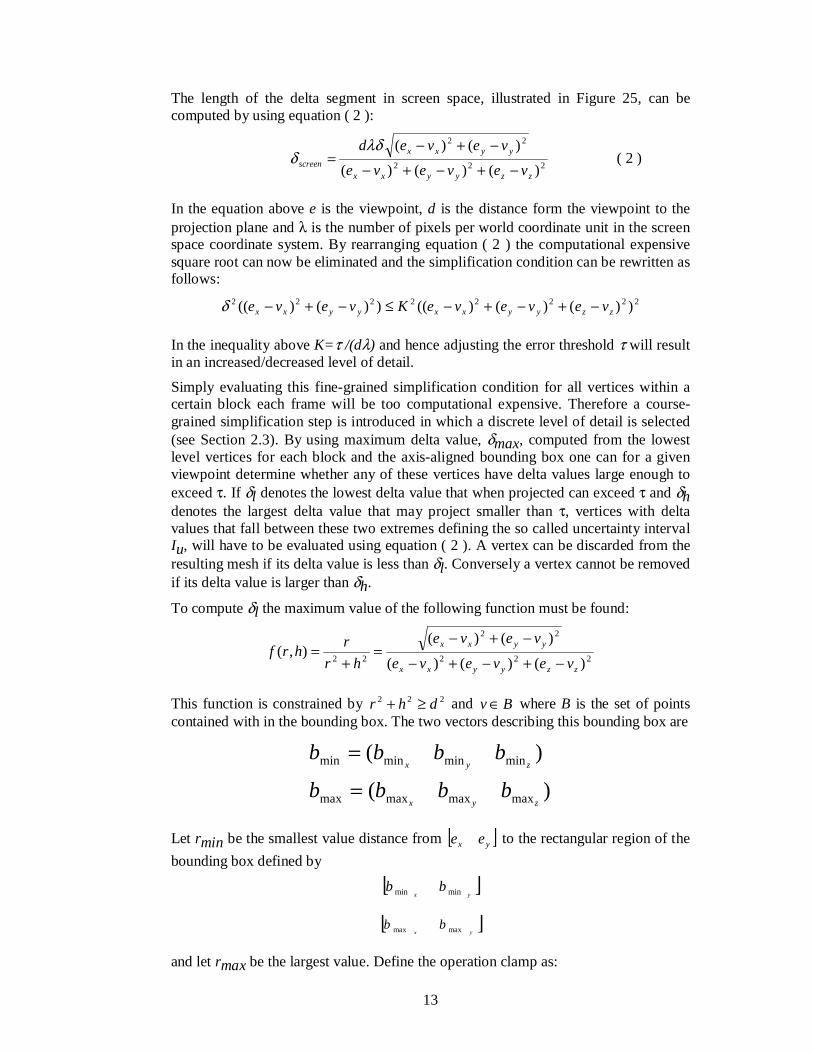
The length of the delta segment in screen space, illustrated in Figure 25, can be computed by using equation ( 2 ):

222

22

)()()(

)()(

zzyyxx

yyxx

screenveveve

veved

−+−+−

−+−=

λδδ ( 2 )

In the equation above e is the viewpoint, d is the distance form the viewpoint to the projection plane and λ is the number of pixels per world coordinate unit in the screen space coordinate system. By rearranging equation ( 2 ) the computational expensive square root can now be eliminated and the simplification condition can be rewritten as follows:

22222222 ))()()(())()(( zzyyxxyyxx veveveKveve −+−+−≤−+−δ

In the inequality above K=τ /(dλ) and hence adjusting the error threshold τ will result in an increased/decreased level of detail.

Simply evaluating this fine-grained simplification condition for all vertices within a certain block each frame will be too computational expensive. Therefore a course-grained simplification step is introduced in which a discrete level of detail is selected (see Section 2.3). By using maximum delta value, δmax, computed from the lowest level vertices for each block and the axis-aligned bounding box one can for a given viewpoint determine whether any of these vertices have delta values large enough to exceed τ. If δl denotes the lowest delta value that when projected can exceed τ and δh denotes the largest delta value that may project smaller than τ, vertices with delta values that fall between these two extremes defining the so called uncertainty interval Iu, will have to be evaluated using equation ( 2 ). A vertex can be discarded from the resulting mesh if its delta value is less than δl. Conversely a vertex cannot be removed if its delta value is larger than δh.

To compute δl the maximum value of the following function must be found:

222

22

22 )()()(

)()(),(

zzyyxx

yyxx

veveve

veve

hr

rhrf

−+−+−

−+−=

+=

This function is constrained by 222 dhr ≥+ and Bv ∈ where B is the set of points contained with in the bounding box. The two vectors describing this bounding box are

)(

)(

maxmaxmaxmax

minminminmin

zyx

zyx

bbbb

bbbb

=

=

Let rmin be the smallest value distance from [ ]yx ee to the rectangular region of the

bounding box defined by

[ ]yx

bb minmin

[ ]yx

bb maxmax

and let rmax be the largest value. Define the operation clamp as:

14

⎪⎭

⎪⎬

⎫

⎪⎩

⎪⎨

⎧

><

=otherwisex

xxifx

xxifx

xxxclamp maxmax

minmin

maxmin ),,(

By setting

|),,(| maxminmin zzbebclampehh zz −==

the maximum value fmax of f(r, h) is found at r=h. If no vertex v exists under the given constraint that satisfies r=h then r is increased/decreased until Bv ∈ . In other words ),,( maxmin rhrclampr = .

In contrast to maximizing the function f(r, h) in order to find δl the same function has to be minimized to find δh. By setting

|}||,max{| maxminmax zzbebehh zz −−==

fmin can be found either when r=rmin or r=rmax, whichever yields a smaller f(r, h).

The bounds on Iu can now be found using equations ( 3 ) and ( 4 ):

maxfdl λτδ = ( 3 )

⎪⎪

⎩

⎪⎪

⎨

⎧

∞

>>

=

=

otherwise

fandiffd

if

h 00

00

minmin

τλτ

τ

δ ( 4 )

By recursively comparing whether δmax<δl the current block is substituted by a lower resolution level of detail block. If on the other hand δmax>δl it may be that a higher resolution block is needed.

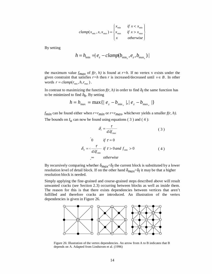
Simply applying the fine-grained and course-grained steps described above will result unwanted cracks (see Section 2.3) occurring between blocks as well as inside them. The reason for this is that there exists dependencies between vertices that aren’t fulfilled and therefore cracks are introduced. An illustration of the vertex dependencies is given in Figure 26.

Figure 26: Illustration of the vertex dependencies. An arrow from A to B indicates that B depends on A. Adapted from Lindstrom et al. (1996)

15

The merging of a triangle pair is only possible if the triangle pair appears on the same level in the triangle subdivision. The process of merging triangles can be viewed as the removal of the common base vertex as illustrated below in Figure 27.

Figure 27: Illustration of the merging process by base vertex removal. After merging the original four triangles are reduced to two triangles.

The mapping of vertices to triangle pairs results in a vertex tree where each node, except for the root and leaves as well as the vertices on the edges of the block, has two parents and four decedents. If any of the decedents of a vertex v is included in the rendered mesh, so is v. In other words v is said to be enabled. To solve the occurrence of cracks between adjacent blocks vertices may be labeled as locked. The result of this is that vertices on the boundaries of the higher resolution block may have to be permanently disabled during simplification.

As with all block-based algorithms extra software can be used to support terrains larger than main memory. This is done by paging blocks in and out of memory when needed/not needed by the algorithm. Lindstrom et al. (1996) describes no such mechanism.

2.4.2 Real-time optimally adapting meshes

The Real-time optimally adapting meshes (ROAM) presented by Duchaineau et al. (1997) is an algorithm that since its publication in 1997 has been widely used in games (Youbing et al. 2001). In this algorithm the triangle bintree structure constitutes the central component of which the first few levels are illustrated in Figure 28.

Figure 28: Illustration of the levels 0-3 of a triangle bintree. Adapted from Duchaineau et al. (1997)

16

In Figure 28 T denotes the root triangle which is a right-isosceles triangle at the coarsest level of subdivision. A right isosceles triangle is a triangle where two of the interior angles are equivalent and the third equals 90o. In order to produce the next-finest level of the bintree the root triangle T is split into two smaller child triangles (T0, T1) separated by the edge stretching form the root triangle’s apex va to the center vc of its base edge (v0, v1). To produce the rest of the triangle bintree this process is repeated recursively until the finest level of detail is reached.

Changing of a bintree triangulation can be performed using two different operations, split and merge. The consequence of using these operations is illustrated in Figure 29.

Figure 29: Illustration of the result produced by the split and merge operations respectively. Adapted from Duchaineau et al. (1997).

As illustrated above the split operation replaces a triangle T with its children (T0, T1), and TB with (TB0, TB1). Figure 29 also illustrates the relationship between the triangles in the neighborhood of T where TB is the base neighbor of T and TL and TR are the left- and right neighbors respectively. Another important fact about triangle bintrees that also is show in Figure 29 is that the neighbors are either from the same bintree level l as T, or from the next finer level l+1 for the left and right neighbors, or from the next courser level l-1 for the base neighbor. If the triangles T and TB are from the same bintree level they are said to form a diamond.

If cracks are to be prevented from occurring between neighboring triangles a triangle T cannot be split directly if its base neighbor TB is from a courser level. Therefore the base neighbor TB must be forced to split before T. As illustrated in Figure 30 the forced split of the base neighbor TB may trigger forced splitting of other triangles.

17

Figure 30: Illustration of the concept of forced splitting. The splitting of the triangle T triggers a series of forced splits starting at TB and ending with a split of the two largest triangles. Adapted from Duchaineau et al. (1997).

To drive the split and merge operations the algorithm utilizes two priority queues, one for each operation. The content of these queues are the triangles, ordered by priority that needs to be split or merged respectively. The advantage of using a second priority queue for mergable diamonds is that it enables the algorithm to exploit frame-to-frame coherence by allowing the algorithm to start from a previously optimal triangulation.

In order to make the algorithm work properly the priorities must be monotonic which means that a child’s priority cannot be large that its parents. To compute the queue priorities a bound per triangle must be used. An example of such a bound is a wedgie (illustrated in Figure 31), defined as the volume of world space containing points (x, y, z) such that (x, y) ∈ T and |z-zT(x, y)| ≤ eT for some wedgie thickness eT.

Figure 31: Illustration of a pair of triangles and the bounding wedgie in which they are contained.

The nested wedgie thickness can now be computed in a bottom-up fashion as follows:

⎩⎨⎧

−+=

otherwise|)()(|),max(

levelfinest at the0

10 cTcTTT vzvzee

e

Using the wedgie thickness the screen space error that also is the triangles priority can be computed using equation ( 5 ):

18

|,|)(

cr

bq

cr

bq

cr

ap

cr

apvdist

−−−

++

−−−

++= ( 5 )

In equation ( 5 ) above (p, q, r) are the camera space coordinates of the vertex v and (a, b, c) is the camera space vector corresponding to the world-space thickness vector (0, 0, eT). Equation ( 5 ) can be rewritten as illustrated in equation ( 6 ):

2

12222

))()((2

)( cqbrcparcr

vdist −+−−

= ( 6 )

Hence a triangles priority increases with the size of the projected error.

In the introduction of this paper the Duchaineau et al. (1997) explain that a complete system for terrain rendering consists of, among other things, a component to manage disk paging of terrain geometry. Even so no such mechanism is presented and in the conclusion the authors state that this is a critical issue that remains to be solved.

2.4.3 Real-Time generation of continuous levels of detail for height fields

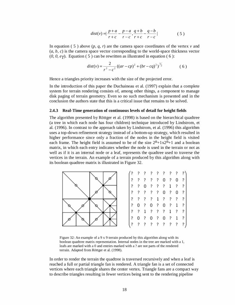
The algorithm presented by Röttger et al. (1998) is based on the hierarchical quadtree (a tree in which each node has four children) technique introduced by Lindstrom, et al. (1996). In contrast to the approach taken by Lindstrom, et al. (1996) this algorithm uses a top-down refinement strategy instead of a bottom-up strategy, which resulted in higher performance since only a fraction of the nodes in the height field is visited each frame. The height field is assumed to be of the size 2n+1x2n+1 and a boolean matrix, in which each entry indicates whether the node is used in the terrain or not as well as if it is an internal node or a leaf, represents the quadtree used to traverse the vertices in the terrain. An example of a terrain produced by this algorithm along with its boolean quadtree matrix is illustrated in Figure 32.

Figure 32: An example of a 9 x 9 terrain produced by this algorithm along with its boolean quadtree matrix representation. Internal nodes in the tree are marked with a 1, leafs are marked with a 0 and entries marked with a ? are not parts of the rendered terrain. Adapted from Röttger et al. (1998).

In order to render the terrain the quadtree is traversed recursively and when a leaf is reached a full or partial triangle fan is rendered. A triangle fan is a set of connected vertices where each triangle shares the center vertex. Triangle fans are a compact way to describe triangles resulting in fewer vertices being sent to the rendering pipeline

19

compared to usual method to describe triangles. An example of a triangle fan is illustrated below in Figure 33.

Figure 33: Illustration of a triangle fan, the primary geometric primitive used for rendering of the quadtree leaves.

In Figure 33 the starting triangle sends vertices v0, v1 and v2 (in that order) but for the following triangles only the next vertex, in this case v3, is sent since it is being used together with the center vertex as well as the previously sent vertex to from a new triangle.

Using this method as is would result in cracks occurring between adjacent blocks of different detail levels (se Section 2.3). Simply skipping the center vertex at these edges prevents this (Röttger et al, 1998). In order for this technique to work the difference in detail level between adjacent blocks can be at most one. How this is solved will be explained shortly.

When performing the refinement step of the algorithm the following two criterions need to be fulfilled. First, the level of detail should decrease as the distance to the viewpoint increases. Second, the level of detail should be higher for regions with high surface roughness. These criterions are in compliance with the description of LOD in Section 2.3. The surface roughness can be pre-calculated using equation ( 7 ):

||max

12

6..1i

idh

dd

== ( 7 )

In the equation above d is the edge length of the block and dhi is the absolute value of the elevation difference as show in Figure 34:

Figure 34: Illustration of how the surface roughness is measured. Adapted from Röttger et al. (1998)

Using equation ( 7 ) Röttger, et al. (1998) presents the subdivision criterion stated in equation ( 8 ):

20

1

)1,2*max(**<= fifrefine

dcCd

lf

( 8 )

Here l is the distance to the viewpoint, C is the minimum global level of detail and c is the desired global level of detail, which can be used to adjust the level of detail. In order to impose the requirement that the difference in level of detail between adjacent blocks cannot be larger than 1 for the crack prevention technique explained earlier to work the pre-calculation of the d2-values must be performed in the following manner. Calculate the local d2-values of all blocks and propagate them up the tree, starting at the smallest existing block. The d2-value of each block is the maximum of the local value and K times the previously calculated values of adjacent blocks at the next lower level. The constant K can be calculated using the minimum global level of detail as stated in equation ( 9 ):

)1(2 −=

C

CK ( 9 )

In order to be able to render terrains that do not entirely fit into main memory Röttger et al. (1998) explain the need of an explicit paging mechanism but no such mechanism is presented.

2.4.4 A fast algorithm for large scale terrain walkthrough

The algorithm presented by Youbing et al. (2001) is based on regular grids as well as the division of large terrains into smaller blocks and it implements a very simple and fast way to prevent cracks between different levels of detail. One common way to perform crack prevention in algorithms based on top-down refinement such as this one is by recursively splitting of neighborhood triangles (see Figure 35). Recursive splitting has the disadvantage of introducing unnecessary triangles and instead this algorithm simply alters the elevation of the vertex that is on the crack as illustrated in Figure 35. The disadvantage of this method is that it causes so-called T-junctions because of the floating-point inaccuracy, which results in a noticeable “missing pixels” effect.

Figure 35: Illustration of two different approaches to crack prevention. On the left cracks are prevented through recursive splitting and on the right through elevation alternation. Adapted from Youbing et al. (2001)

The refinement method used in this algorithm is a hybrid of the block based quad subdivision method used by Lindstrom et al. (1996) and the right isosceles based

21

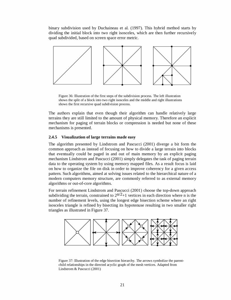
binary subdivision used by Duchaineau et al. (1997). This hybrid method starts by dividing the initial block into two right isosceles, which are then further recursively quad subdivided, based on screen space error metric.

Figure 36: Illustration of the first steps of the subdivision process. The left illustration shows the split of a block into two right isosceles and the middle and right illustrations shows the first recursive quad subdivision process.

The authors explain that even though their algorithm can handle relatively large terrains they are still limited to the amount of physical memory. Therefore an explicit mechanism for paging of terrain blocks or compression is needed but none of these mechanisms is presented.

2.4.5 Visualization of large terrains made easy

The algorithm presented by Lindstrom and Pascucci (2001) diverge a bit form the common approach as instead of focusing on how to divide a large terrain into blocks that eventually could be paged in and out of main memory by an explicit paging mechanism Lindstrom and Pascucci (2001) simply delegates the task of paging terrain data to the operating system by using memory mapped files. As a result focus is laid on how to organize the file on disk in order to improve coherency for a given access pattern. Such algorithms, aimed at solving issues related to the hierarchical nature of a modern computers memory structure, are commonly referred to as external memory algorithms or out-of-core algorithms.

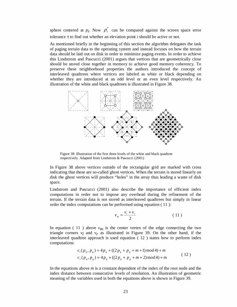
For terrain refinement Lindstrom and Pascucci (2001) choose the top-down approach subdividing the terrain, constrained to 2n/2+1 vertices in each direction where n is the number of refinement levels, using the longest edge bisection scheme where an right isosceles triangle is refined by bisecting its hypotenuse resulting in two smaller right triangles as illustrated in Figure 37.

Figure 37: Illustration of the edge bisection hierarchy. The arrows symbolize the parent-child relationships in the directed acyclic graph of the mesh vertices. Adapted from Lindstrom & Pascucci (2001)

22

The triangle mesh produced by this bisection scheme can be viewed as a directed acyclic graph where an edge (i, j) represents a bisection of a triangle where j is inserted on the hypoteneous and connected to i at the right angle corner of the triangle. In order to produce a continuous terrain without T-junctions and cracks the following properties must be satisfied:

MiMj ∈⇒∈ iCj ∈

Here M represents a given refinement and Ci is the set of children of i. This property implies that if an elevation point j is active so must its parent. To ensure the satisfaction of this property the following condition must apply:

),,(),,( epep jjii δρδρ ≥ iCj ∈∀

In the condition above ρ is the projected screen space error term, pi is the position of the vertex i, δi is an object space error term for i and e is the viewpoint. Hence ρ consists of two different parts, which are the object space error term, δi and a view-dependent term that relates pi and e. As mentioned above the error terms must be nested to guarantee that a parent is active if any of its children is active. Nesting of the object space error term δi can therefore be calculated in the following manner:

⎪⎩

⎪⎨

⎧=

∈ iCjji

i

i }}max{,max{ **

δδδ

δ

This does not guarantee ρ(δi*, pi, e) ≥ ρ(δj*, pj, e) for j ∈ Ci because the viewer might be close to the child pj and far from parent pi. To solve this Lindstrom and Pascucci (2001) uses a nested hierarchy of nested spheres by defining a ball Bi of radius ri centered on pi where ri is calculated in the following manner:

⎪⎩

⎪⎨⎧

+−=∈

}|{|max

0

jjiCj

i rppri

The adjusted projected error can now be written as

),,(max ** exiBx

ii

δρρ∈

=

It is important to mention that this is the general framework for refinement and that the algorithm is virtual independent of the error metric being used. Even so Lindstrom and Pascucci (2001) describe the projected error metric used by their terrain visualization system, which is stated in equation ( 10 ) :

ii

ii rep −−

=||

** δλρ ( 10 )

In equation ( 10 ) above λ=w/ϕ where w is the number of pixels along the field of view ϕ, pi is the vertex being evaluated, e is the viewpoint and ri is the radius of the

if i is a leaf node

otherwise

if i is a leaf node

otherwise

23

sphere centered at pi. Now *iρ can be compared against the screen space error

tolerance τ to find out whether an elevation point i should be active or not.

As mentioned briefly in the beginning of this section the algorithm delegates the task of paging terrain data to the operating system and instead focuses on how the terrain data should be laid out on disk in order to minimize paging events. In order to achieve this Lindstrom and Pascucci (2001) argues that vertices that are geometrically close should be stored close together in memory to achieve good memory coherency. To preserve these neighborhood properties the authors introduced the concept of interleaved quadtrees where vertices are labeled as white or black depending on whether they are introduced at an odd level or an even level respectively. An illustration of the white and black quadtrees is illustrated in Figure 38.

Figure 38: Illustration of the first three levels of the white and black quadtree respectively. Adapted from Lindstrom & Pascucci (2001)

In Figure 38 above vertices outside of the rectangular grid are marked with cross indicating that these are so-called ghost vertices. When the terrain is stored linearly on disk the ghost vertices will produce “holes” in the array thus leading a waste of disk space.

Lindstrom and Pascucci (2001) also describe the importance of efficient index computations in order not to impose any overhead during the refinement of the terrain. If the terrain data is not stored as interleaved quadtrees but simply in linear order the index computations can be performed using equation ( 11 ):

2rl

m

vvv

+= ( 11 )

In equation ( 11 ) above vm is the center vertex of the edge connecting the two triangle corners vl and vr as illustrated in Figure 39. On the other hand, if the interleaved quadtree approach is used equation ( 12 ) states how to perform index computations:

mmpppppc

mmpppppc

gqqgqr

gqqgql

+++++=+++++=

)4mod)22((4),(

)4mod)12((4),( ( 12 )

In the equations above m is a constant dependent of the index of the root node and the index distance between consecutive levels of resolution. An illustration of geometric meaning of the variables used in both the equations above is shown in Figure 39.

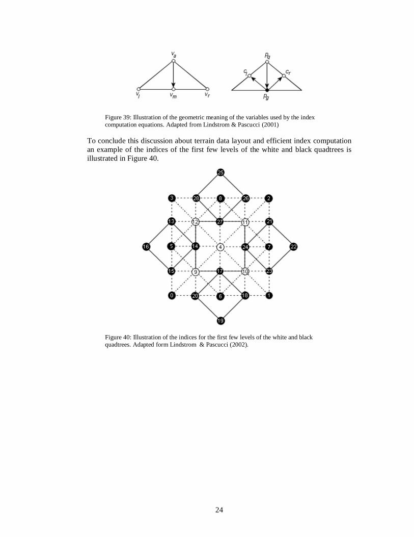
24

Figure 39: Illustration of the geometric meaning of the variables used by the index computation equations. Adapted from Lindstrom & Pascucci (2001)

To conclude this discussion about terrain data layout and efficient index computation an example of the indices of the first few levels of the white and black quadtrees is illustrated in Figure 40.

Figure 40: Illustration of the indices for the first few levels of the white and black quadtrees. Adapted form Lindstrom & Pascucci (2002).

25

3 Problem Ericsson Microwave Systems (EMW) in Skövde, a member of the Ericsson group provides a professional competence as well as resource reinforcement in the field of software engineering. A part of EMW: s activity is to develop simulators that with high accuracy can reproduce radar functionality. In order to evaluate the results of a simulation, manual analysis of tables of simulation data is conducted a tedious process for large simulations. Therefore EMW seek to incorporate three-dimensional graphics into their simulators to extend these with the ability to provide the operator with visual feedback during a simulation.

In these simulators it is important to be able to verify the surrounding environment, consisting of three-dimensional terrain data, in which the simulation takes place. EMW is looking for a terrain-rendering algorithm that meets the following requirements.

1. The algorithm should be able to handle terrain data that is larger than main memory of a single personal computer.

2. The algorithm should be able to adjust the level of detail of the terrain if the load on other relatively more critical parts of the system exceeds some threshold.

The latter requirement is important since, even though terrain rendering constitutes a central component of these simulators, it is important that the simulator’s performance is not compromised because of the complex surroundings. The increase in system load can be due to an increase in the number of targets entering the simulations.

3.1 Problem definition

A lot of different algorithms for terrain rendering have been developed during the last decades all with their own set of pros and cons. The aim of this paper is to identify and evaluate those algorithms that conform to EMW: s requirements. This aim is broken down into the following objectives to (i) perform a litterateur survey over existing algorithms in order to find those algorithms that fit EMW: s needs, (ii) to implement these algorithms and (iii) develop a test environment in which these algorithms can be evaluated from a performance perspective.

3.2 Delimitation

My work is solely concentrated on finding those algorithms that best satisfies EMW: s requirements, to implement and evaluate these algorithms from a performance perspective. The algorithms should be able to meet the requirements “as is” without modification as well as extra functionality.

3.3 Expected result

My expectation is to find at least one algorithm that will meet EMW: s requirements and I expect to be able to show that this or these algorithms will have a positive impact on EMW: s simulators.

26

4 Method To evaluate the performance of the algorithms tests will be conducted on a specified test architecture using combinations of test cases designed to measure the algorithm performance. The configuration of the test architecture is explained in Section 4.1 and the different test cases will be stated in Section 4.2

4.1 Test architecture

The test architecture used for testing of the algorithms is constituted by a Dell Optiplex GX240 equipped with a Intel Pentium 4 1.8 GHz processor, 513 MB RAM, 36 GB IDE HD and a Hercules 3D Prophet II Geforce 2 GTS Pro 64MB graphics card. The operating system running on this machine is Mandrake Linux version 8.0 and it uses OpenGL, an application programming interface (API) developed by SGI in 1992, for rendering as well as the OpenGL Utility Toolkit (GLUT), a simple windowing API for window management. The compiler used by the test architecture is the GNU Compiler Collection (GCC) version 2.96 and common to all tests is the window size of 800x600 pixels as well as 60 degrees field-of-view (see Section2.1).

4.2 Test cases The following sections describe the different test cases that will be used to test the performance of the algorithms. In Section 4.2.1 the terrain used through all test cases is described followed by a description of the fly-over path in Section 4.2.2. Section 4.2.3 discusses the four different operations that will be tested and Section 4.2.4 deals with the test case involving different memory configurations.

4.2.1 Terrain

The terrain used to test the algorithms is the one used by Lindstrom and Pascucci (2001). This terrain, a subset of the original terrain provided by The United States Geological Survey (USGS), with the dimensions 16385x16385 pixels uses an inter-pixel spacing of 10 meters as well as maximum height of 6553.5 meters. The motivation for using this terrain is that in contains both flat and rough regions, which when flown over will provide results on how dependent the algorithm performance is of the underlying terrain complexity. The terrain is illustrated in Section 11.

4.2.2 Path

When flying over the terrain a similar path is taken through all test cases. By attaching the camera onto a mathematical curve called a Hermite spline (named after the Frence mathematician Charles Hermite) a terrain fly-over can be performed. The path is formed like a double eight and it constitutes a good fly-over path as it passes over both rough and flat regions of the terrain. The fly-over path is illustrated in Figure 41.

27

Figure 41: Illustration of the path used for terrain fly-over

4.2.3 Operation

Section 1 state that simple brute force rendering of large terrains will not work. To solve this Sections 2.2 and 2.3 introduced the concept of view frustum culling and LOD respectively. To verify the need for these techniques the following tests will be conducted by (i) rendering the terrain using brute force, (ii) rendering the terrain using only view frustum culling, (iii) rendering the terrain using only LOD and (iv) rendering the terrain using both view frustum culling and LOD.

4.2.4 Physical memory

To measure how the amount of available physical memory affects the performance of the algorithm tests will be conducted using variable amounts of RAM. Since the maximum amount of physical memory available on the test architecture is 512 MB the test cases will include 128 MB, 256 MB and 512 MB of RAM. These memory configurations will provide results on how dependent the algorithms performance is on the amount of available physical memory.

28

5 Implementation

5.1 Algorithm selection

Among those algorithms accounted for in Section 2.4 the one presented by Lindstrom and Pascucci (2001) is the only algorithm that “as is” meets EMW: s requirements. All other algorithms described in Section 2.4 require extra software in form of an explicit paging mechanism to be able to handle large terrains but no such mechanism is described by any of the authors. The approach taken by Lindstrom and Pascucci (2001) is to delegate the task of paging terrain data to the operating system and instead focusing on how to organize the terrain data on disk to reduce the amount of paging events. The source code of the implementation of this algorithm is presented in Section 12.

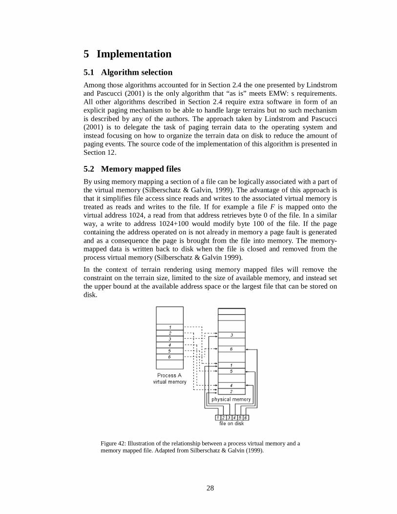
5.2 Memory mapped files

By using memory mapping a section of a file can be logically associated with a part of the virtual memory (Silberschatz & Galvin, 1999). The advantage of this approach is that it simplifies file access since reads and writes to the associated virtual memory is treated as reads and writes to the file. If for example a file F is mapped onto the virtual address 1024, a read from that address retrieves byte 0 of the file. In a similar way, a write to address 1024+100 would modify byte 100 of the file. If the page containing the address operated on is not already in memory a page fault is generated and as a consequence the page is brought from the file into memory. The memory-mapped data is written back to disk when the file is closed and removed from the process virtual memory (Silberschatz & Galvin 1999).

In the context of terrain rendering using memory mapped files will remove the constraint on the terrain size, limited to the size of available memory, and instead set the upper bound at the available address space or the largest file that can be stored on disk.

Figure 42: Illustration of the relationship between a process virtual memory and a memory mapped file. Adapted from Silberschatz & Galvin (1999).

29

5.3 Additional test cases

The choice of algorithm resulted in the production of two additional test cases, which are presented below in Sections 5.3.1 and 5.3.2 respectively. This also resulted in a restriction on terrain size described in Section 5.3.3 as well as a change of possible memory configurations discussed in Section 5.3.4.

5.3.1 File layout

Since the performance of the selected algorithm is dependent of how the terrain data is laid out on disk two different file layouts will be compared. The first layout is the simple linear array layout and the second the more advanced interleaved quadtree layout both described in Section 2.4.5. The purpose of this test is to measure how much performance is to be gained by using the latter layout compared to the former and thereby establishing whether the somewhat disk wasting interleaved quadtree layout is really worthwhile. The thesis is that the importance of the quadtree file layout decreases as the amount of available physical memory increases and therefore this test will be performed in conjunction with the variable physical memory tests described in Section 4.2.4.

5.3.2 Adjustable error metric

The second requirement described in Sections 1 and 3 states that the algorithm should have a configurable error metric that could be adjusted in order to increase or decrease the level of detail depending on the system stress. To measure how the allowable screen space error affects the algorithms performance test will be conducted with the screen space error threshold set to 1, 2, 4 and 8 pixels.

5.3.3 Terrain revisited

The available address space on test architecture in conjunction with disk space consumed by the algorithms imposes a restriction on the maximum size of the terrain that can be used when testing the algorithm performance. Since the original terrain contains 16385x16385 vertices the file used to test the algorithm will be approximately 5 GB as the algorithm stores 20 bytes per vertex. A file of this size cannot be addressed using a 32-bit architecture since the address space is limited to 232 = 4 GB. To solve this problem the original terrain is scaled down to the next lower size allowed by the algorithm namely 8193x8193 vertices. As the Linux system call mmap, used to memory map a file, cannot be used with files larger than 2 GB neither this terrain can be used since when converted into the quadtree format this file becomes slightly above 2 GB. Therefore the size of the terrain must be further reduced to 4097x4097 vertices. The terrain is illustrated in Section 11.

5.3.4 Physical memory revisited

Because of the limitations on the terrain size described in Section 5.3.3 the test cases involving different sizes of physical memory must be reduced. The reason for this is that a terrain consisting of 4097x4097 vertices consumes about 320 MB of disk space when using the linear file layout but approximately 533 MB when using the quadtree file layout and thus giving the linear file layout an advantaged since the entire file can be loaded into memory. Therefore when evaluating the importance of the amount of physical memory only 128 MB and 256 MB will be used and the results from using 512 MB will be presented in separate diagrams.

30

6 Results and analysis This section covers the results obtained through testing of the selected algorithm. All tests consisted of a 5000 frame terrain fly-over, using the path described in Section 4.2.2, flown three times and the results presented in the diagrams are the average of these three fly-overs.

An important note concerning the tests involving measurements of each frame is that for some of these tests the second frame has manually been divided by ten. The reason for this is that during this frame a substantial amount of time was consumed because of the large amount of paging faults (see Section 5.2) resulting in a very coarse-grained y-axis in the diagrams and without this alternation the difference between the curves was hard to observe. It is also important to note that this alternation has no effect on the final result. Further the results in each diagram have been plotted using a Bezier curve in order to make the diagrams more readable. This leads to a loss of precision but since the curves in the diagrams should be compared to each other and not interpreted as absolute values this has little effect on the results.

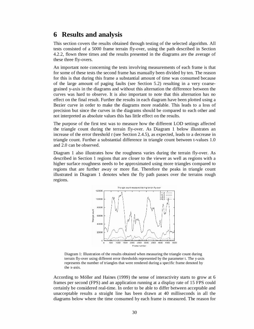
The purpose of the first test was to measure how the different LOD settings affected the triangle count during the terrain fly-over. As Diagram 1 below illustrates an increase of the error threshold t (see Section 2.4.5), as expected, leads to a decrease in triangle count. Further a substantial difference in triangle count between t-values 1.0 and 2.0 can be observed.

Diagram 1 also illustrates how the roughness varies during the terrain fly-over. As described in Section 1 regions that are closer to the viewer as well as regions with a higher surface roughness needs to be approximated using more triangles compared to regions that are further away or more flat. Therefore the peaks in triangle count illustrated in Diagram 1 denotes when the fly path passes over the terrains rough regions.

Diagram 1: Illustration of the results obtained when measuring the triangle count during terrain fly-over using different error thresholds represented by the parameter t. The y-axis represents the number of triangles that were rendered during a specific frame denoted by the x-axis.

According to Möller and Haines (1999) the sense of interactivity starts to grow at 6 frames per second (FPS) and an application running at a display rate of 15 FPS could certainly be considered real-time. In order to be able to differ between acceptable and unacceptable results a straight line has been drawn at 40 milliseconds in all the diagrams below where the time consumed by each frame is measured. The reason for

31

this is that if each frame consumes 40 milliseconds the results is 25 FPS, which is the frame rate, used by the European TV standard PAL (Marchall, 1995). This is also the frame rate used by Röttger et al. (1998) for testing of their algorithm.

The second test aimed to evaluate the performance gains when using view frustum culling as well as LOD, explained in Sections 2.2 and 2.3 respectively, compared to brute force rendering. In Diagram 2 below the results from the fly-over using brute force rendering as well as using only view frustum culling has been omitted. The reason for this is that when using brute force rendering not a single frame was produced during the first five minutes and therefore the test was aborted. This further strengthens the statement made in Section 1 that brute force rendering will not work for large terrain. Similar, the view frustum-culling test had a hard time completing a single lap and when one and a half hour had passed this test was aborted as well. As the diagram illustrates it is possible to perform a fly-over using only LOD but the result is hardly satisfactory. This could of course be solved by increasing the error threshold but would also lead to an unacceptably low detail level. Further the diagram illustrates that using LOD in conjunction with view frustum culling can make a substantial performance increase. In these test the error threshold t was set to 1.0.

Diagram 2: Illustration of the results obtained when performing terrain fly-over using the different rendering operations. In the diagram no results using brute force rendering as well as only view frustum culling are presented since these rendering operations was not able to produce any results.

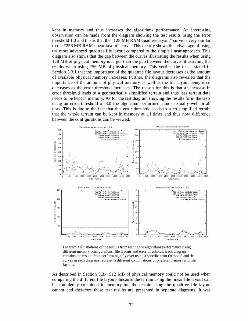
As described in Section 2.4.5 the approach taken by Lindstrom and Pascucci (2001) is to delegate the task of paging terrain data to the operating system and instead focusing on how to arrange the terrain data on disk to minimize the amount of page faults. The purpose of the third test is to see how much impact the amount of physical memory has on the algorithms performance when using the two different file layouts, described in Section 2.4.5, in conjunction with the different error thresholds described in Section 5.3.2. The four diagrams obtained through these tests are shown below. As illustrated by these diagrams the algorithm have a hard time meeting the time requirements, described above when the error threshold is set to 1.0. When the error threshold is increased to 2.0 all configurations except “128 MB RAM linear layout” manage to meet the time requirements during nearly the entire fly over. Relating this result to the result in Diagram 1 increasing the error threshold from 1.0 to 2.0 leads to a large reduction of the triangle count and thus by sacrificing geometric detail more performance can be gained.

As expected, more physical memory is beneficial, especially when using a low error threshold, since it reduces the amount of page faults as more memory pages can be

32

kept in memory and thus increases the algorithms performance. An interesting observation can be made from the diagram showing the test results using the error threshold 1.0 and this is that the “128 MB RAM quadtree layout” curve is very similar to the “256 MB RAM linear layout” curve. This clearly shows the advantage of using the more advanced quadtree file layout compared to the simple linear approach. This diagram also shows that the gap between the curves illustrating the results when using 128 MB of physical memory is larger than the gap between the curves illustrating the results when using 256 MB of physical memory. This verifies the thesis stated in Section 5.3.1 that the importance of the quadtree file layout decreases as the amount of available physical memory increases. Further, the diagrams also revealed that the importance of the amount of physical memory as well as the file layout being used decreases as the error threshold increases. The reason for this is that an increase in error threshold leads to a geometrically simplified terrain and thus less terrain data needs to be kept in memory. As for the last diagram showing the results form the tests using an error threshold of 8.0 the algorithm performed almost equally well in all tests. This is due to the fact that this error threshold leads to such simplified terrain that the whole terrain can be kept in memory at all times and thus now difference between the configurations can be viewed.

Diagram 3 Illustrations of the results from testing the algorithms performance using different memory configurations, file layouts and error thresholds. Each diagram contains the results from performing a fly over using a specific error threshold and the curves in each diagrams represents different combinations of physical memory and file layouts.

As described in Section 5.3.4 512 MB of physical memory could not be used when comparing the different file layouts because the terrain using the linear file layout can be completely contained in memory but the terrain using the quadtree file layout cannot and therefore these test results are presented in separate diagrams. It was

33

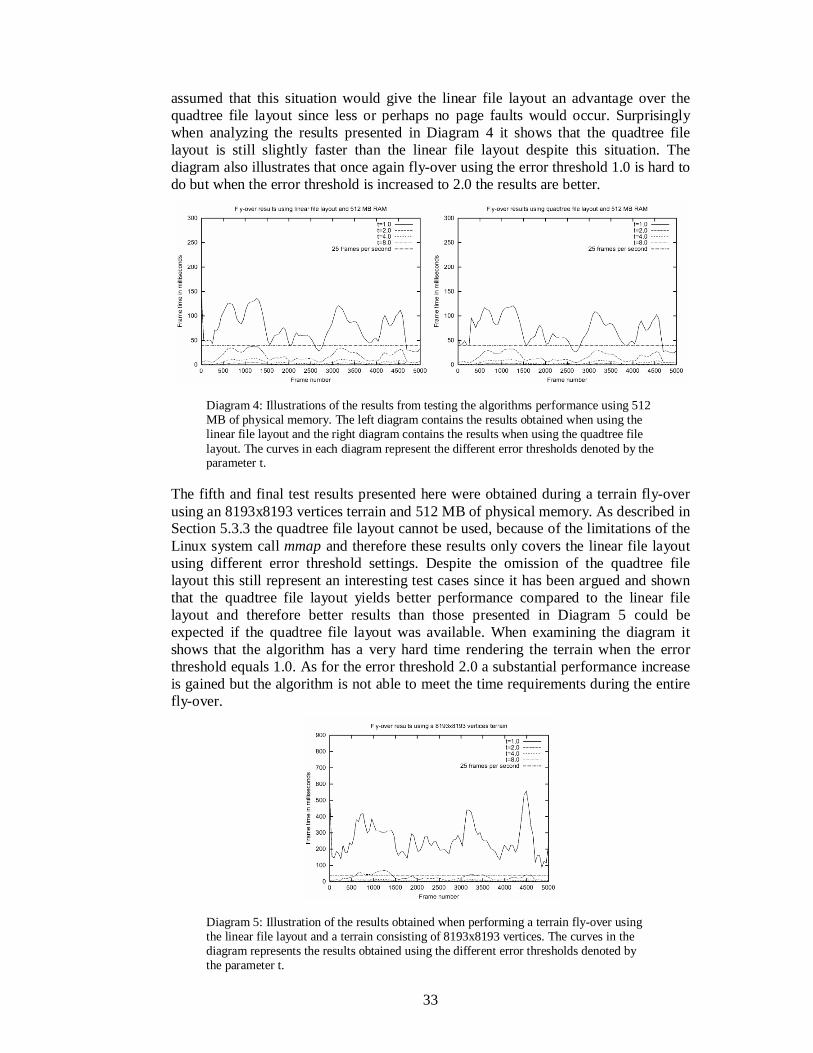
assumed that this situation would give the linear file layout an advantage over the quadtree file layout since less or perhaps no page faults would occur. Surprisingly when analyzing the results presented in Diagram 4 it shows that the quadtree file layout is still slightly faster than the linear file layout despite this situation. The diagram also illustrates that once again fly-over using the error threshold 1.0 is hard to do but when the error threshold is increased to 2.0 the results are better.

Diagram 4: Illustrations of the results from testing the algorithms performance using 512 MB of physical memory. The left diagram contains the results obtained when using the linear file layout and the right diagram contains the results when using the quadtree file layout. The curves in each diagram represent the different error thresholds denoted by the parameter t.

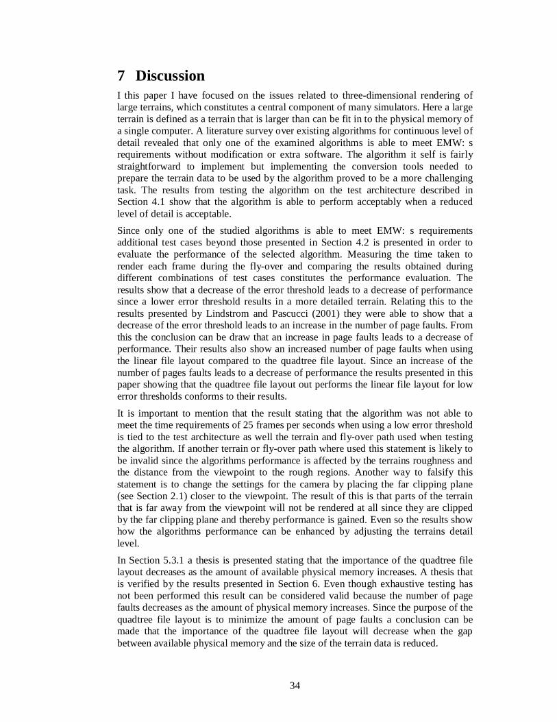
The fifth and final test results presented here were obtained during a terrain fly-over using an 8193x8193 vertices terrain and 512 MB of physical memory. As described in Section 5.3.3 the quadtree file layout cannot be used, because of the limitations of the Linux system call mmap and therefore these results only covers the linear file layout using different error threshold settings. Despite the omission of the quadtree file layout this still represent an interesting test cases since it has been argued and shown that the quadtree file layout yields better performance compared to the linear file layout and therefore better results than those presented in Diagram 5 could be expected if the quadtree file layout was available. When examining the diagram it shows that the algorithm has a very hard time rendering the terrain when the error threshold equals 1.0. As for the error threshold 2.0 a substantial performance increase is gained but the algorithm is not able to meet the time requirements during the entire fly-over.

Diagram 5: Illustration of the results obtained when performing a terrain fly-over using the linear file layout and a terrain consisting of 8193x8193 vertices. The curves in the diagram represents the results obtained using the different error thresholds denoted by the parameter t.

34

7 Discussion I this paper I have focused on the issues related to three-dimensional rendering of large terrains, which constitutes a central component of many simulators. Here a large terrain is defined as a terrain that is larger than can be fit in to the physical memory of a single computer. A literature survey over existing algorithms for continuous level of detail revealed that only one of the examined algorithms is able to meet EMW: s requirements without modification or extra software. The algorithm it self is fairly straightforward to implement but implementing the conversion tools needed to prepare the terrain data to be used by the algorithm proved to be a more challenging task. The results from testing the algorithm on the test architecture described in Section 4.1 show that the algorithm is able to perform acceptably when a reduced level of detail is acceptable.

Since only one of the studied algorithms is able to meet EMW: s requirements additional test cases beyond those presented in Section 4.2 is presented in order to evaluate the performance of the selected algorithm. Measuring the time taken to render each frame during the fly-over and comparing the results obtained during different combinations of test cases constitutes the performance evaluation. The results show that a decrease of the error threshold leads to a decrease of performance since a lower error threshold results in a more detailed terrain. Relating this to the results presented by Lindstrom and Pascucci (2001) they were able to show that a decrease of the error threshold leads to an increase in the number of page faults. From this the conclusion can be draw that an increase in page faults leads to a decrease of performance. Their results also show an increased number of page faults when using the linear file layout compared to the quadtree file layout. Since an increase of the number of pages faults leads to a decrease of performance the results presented in this paper showing that the quadtree file layout out performs the linear file layout for low error thresholds conforms to their results.

It is important to mention that the result stating that the algorithm was not able to meet the time requirements of 25 frames per seconds when using a low error threshold is tied to the test architecture as well the terrain and fly-over path used when testing the algorithm. If another terrain or fly-over path where used this statement is likely to be invalid since the algorithms performance is affected by the terrains roughness and the distance from the viewpoint to the rough regions. Another way to falsify this statement is to change the settings for the camera by placing the far clipping plane (see Section 2.1) closer to the viewpoint. The result of this is that parts of the terrain that is far away from the viewpoint will not be rendered at all since they are clipped by the far clipping plane and thereby performance is gained. Even so the results show how the algorithms performance can be enhanced by adjusting the terrains detail level.

In Section 5.3.1 a thesis is presented stating that the importance of the quadtree file layout decreases as the amount of available physical memory increases. A thesis that is verified by the results presented in Section 6. Even though exhaustive testing has not been performed this result can be considered valid because the number of page faults decreases as the amount of physical memory increases. Since the purpose of the quadtree file layout is to minimize the amount of page faults a conclusion can be made that the importance of the quadtree file layout will decrease when the gap between available physical memory and the size of the terrain data is reduced.

35

8 Conclusion A lot of different algorithms for continuous level of detail have been developed during the last decade but of those presented in this paper only one addresses the requirement presented in Section 1 stating that the algorithm should be able to handle terrain data that are larger than main memory of a single personal computer. All the others require extra software in terms of a paging mechanism responsible for bringing terrain data in and out of main memory but no such mechanism is described. The selected algorithm, developed by Lindstrom and Pascucci (2001), delegates the task of paging terrain data to the operating system and instead focuses on how to organize the file on disk in order to minimize the amount of page faults. It has been shown that this algorithm performs fairly well when tested using a large terrain on the specified test architecture described in Section 4.1. Though the algorithm experience some problems when trying to render parts of the terrain with a high level of detail adjusting the error threshold and thereby sacrificing geometry detail has shown to be an effective way to gain further performance. Therefore the algorithm is also able to meet the second requirements presented in Section 1.

As expected the amount of available physical memory has heavy impact on the algorithms performance since more memory reduced the likelihood of page fault as large parts of the terrain can be kept in memory at all times. Further testing also reviled the significance of using the more advanced quadtree file layout compared to the linear file layout as the former out-performed the latter when using a low error threshold. It has also been show that the importance of quadtree file layout decreases as the error threshold increases.

Testing also verified the statement made in Section 1 that the brute force rendering approach does not work for large terrains. Neither by adding view frustum culling resulted in an acceptable performance and the same goes for using only LOD. By combining LOD and view frustum culling the algorithm experienced a substantial performance increase. This comes from the fact that when performing a terrain fly-over the viewer does not see large parts of the terrain and hence there is no point in rendering these parts.

36

9 Future work Future work could be to implement a multithreaded version of the selected algorithm. Lindstrom and Pascucci (2001) explain how this can be done and their results reveals that multithreading leads to a substantial increase in performance when tested on a multi-processor architecture. Testing such an implementation on the test architecture described in Section 4.1 would show whether performance could be gained even on an architecture using a single processor. Such test would also reveal how the visual quality of the simulations is affected since the main thread would be rendering a potentially old version of the terrain until the refinement thread delivers a new refined version.

When dealing with terrain data larger than physical memory there is still a restriction on the largest terrain that can be used imposed by the available address space. On the test architecture described in Section 4.1 the available address space is 4 GB but this amount is reduced due to the 2 GB limitation of mmap. One way to solve this is to migrate from at 32-bit architecture to a 64-bit architecture but this would also lead to a substantial cost increase. Another feasible solution might be to use compressed terrain data and perform decompression at run-time. Testing would show how run-time decompression affects the algorithms performance and thereby determine whether or not such a solution would be acceptable.

Performing a terrain fly-over rendering result in a quite noticeable “popping effect” (see Section 2.3) especially for high error thresholds. Adding geomorphing to the current implementations could minimize this not so visually appealing phenomenon. With geomorphing a vertex is not just omitted when the projected error falls below the error threshold but instead it is gradually lowered or raised before it is removed. This could be viewed as an animated version of the vertex elevation process described in Section 2.4.4. Testing of such a mechanism would reveal its impact on performance as well as whether or not implementing geomorphing is really worth it in terms of enhanced visual experience.

37

10 References Assarsson, U. & Möller, T. (2000) Optimized View frustum culling algorithms for bounding boxes, Journal of Graphics Tools, 5(1), Pages 9-22

Blow, J. (2000) Terrain Rendering at High Levels of Detail. Game Developers' Conference

Design CAD 3D Max (2001) [Computer program] Upperspace Coorp.Availible on the Internet: http://www.upperspace.com/downloads/eval.asp [Retrieved 02.03.10]

Duchaineau, M., Wolinsky, M., Sigeti, D. E., Miller, M. C., Aldrich, Charles. & Mineew-Weinstein, M. B. (1997) ROAMing terrain: Real-time optimally adapting meshes. IEEE Visualization ’97, pages 81-88

Eberly, D. H. (2001) 3D Game engine design: A practical approach to real-time computer graphics Academic Press

Kilgard, M. J. GLUT [Software library] Available on the Internet: http://www.opengl.org/developers/documentation/glut/glut-3.7.tar.gz [Retrieved 02.03.14]

Lindstrom, P., Koller, D., Ribarsky, W., Hodges, L. F., Faust, N. & Turner, G. A. (1996) Real-time, continuous level of detail rendering of height fields. ACM SIGGRAPH 96 Proceedings, pages 109-118

Lindstrom, P. & Pascucci, V. (2001) Visualization of large terrains made easy, IEEE Visualization 2001 Proceedings, pp. 363-370

Lindstrom, P & Pascucci, V (2002) Visualization of large terrains made easy Supplemental information. Available on the Internet: http://www.gvu.gatech.edu/people/peter.lindstrom/papers/visualization2001a/supplenental/ [Retrieved 02.03.07]

Möller, T. & Haines, E. (1999) Real-time rendering, A K Peters Ltd.

Quake 3 (1999) [Computer program], id Software

Röttger, S., Heidrich, W., Slusallek, P. & Seidel H. -P. Real-time generation of continuous levels of detail for height fields. Proceedings of WSCG’98, pages 315-322, 1998

Silberschatz, A. & Galvin, P. B. (1999) Operating system concepts (Fifth edition). John Wiley & Sons, Inc.

Marchall, B (1995) Integration of digital video into distributed hypermedia systems. Masters thesis.

Wolfenstein 3D (1991) [Computer program], id Software, Available on the Internet: ftp://ftp.sunet.se/pub/pc/games/idgames2/levels/v-z/wolf3d.zip [Retrieved 02.03.10]

Wortham, S. Terra3D (2002) [Computer program] Available on the Internet: http://www.stevescomp.atfreeweb.com/programs/ [Retrieved 02.03.10]

Youbing, Z., Ji, Z., Jiaoying, S. & Zhigeng, P. (2001) A fast algorithm for large scale terrain walkthrough. CAD/Graphics’2001

38

11 Appendix A

39

12 Appendix B Testbed.cpp #include <ctime> #include <cstring> #include <stdio.h> #include <GL/glut.h> #include <math3d/m3d.h> #include <math3d/m4x4.h> #include "ccamera.h" #include "cterraindata.h" #include "cterrain.h" #include "chermitespline.h" #include "cpnmbitmap.h" #include "ctimer.h" //Test type enum TestType{MEMORY_TEST, OPERATION_TEST, TRIANGLELOD_TEST}; //Constants const int WINDOW_WIDTH = 800; const int WINDOW_HEIGHT = 600; //Variables TestType testType; //Test type unsigned int noOfSteps; //Number of steps per fly-over lap double stepSize; //Size of each step unsigned int stepCounter = 0; //Keeps track of the number of taken steps char fileName[64]; //Output file filename FILE *outputFile; //Output file file stream unsigned int noOfLaps=0; //Number of fly-overs unsigned int lapNumber=0; //Current fly-over lap unsigned int *results; //Measurment results CCamera* camera; //Camera CTerrainData* td; //Terrain data CTerrain* terrain; //Terrain CHermiteSpline *spline; //Fly-over path CPNMBitmap *bitmap; //Terrain texture CTimer timer; //Timer CTerrain::Mode mode; //Rendering operation //Lighting settings GLfloat globalAmbient[]={0.2, 0.2, 0.2, 1.0}; GLfloat light0Position[]={2048.0, 7000.0, 2048.0, 0.0}; GLfloat light0Ambient[]={0.5, 0.5, 0.5, 1.0}; GLfloat light0Diffuse[]={1.0, 1.0, 1.0, 1.0}; GLfloat light0Specular[] = {1.0, 1.0, 1.0, 1.0}; GLfloat terrainAmbientAndDiffuse[] = { 0.1, 0.4, 0.1, 1.0}; GLuint texture; //Terrain texture object void init(void) { //Setup OpenGL glClearColor(0.0,0.0,0.0,0.0); glShadeModel(GL_FLAT); glEnable(GL_DEPTH_TEST); glLightModelfv(GL_LIGHT_MODEL_AMBIENT, globalAmbient);

40

glLightModeli(GL_LIGHT_MODEL_LOCAL_VIEWER, GL_FALSE); glLightModeli(GL_LIGHT_MODEL_TWO_SIDE, GL_FALSE); glLightfv(GL_LIGHT0, GL_AMBIENT, light0Ambient); glLightfv(GL_LIGHT0, GL_DIFFUSE, light0Diffuse); glLightfv(GL_LIGHT0, GL_SPECULAR, light0Specular); glEnable(GL_LIGHTING); glEnable(GL_LIGHT0); glEnable(GL_NORMALIZE); glEnable(GL_CULL_FACE); glCullFace(GL_FRONT); //Create a new camera camera = new CCamera(CVector3f(0.0, 50.0, 0.0), CVector3f(0.0, 0.0, 1.0), CVector3f(0.0, 1.0, 0.0), 60.0, 1.0, 1000000.0, static_cast<GLdouble> (WINDOW_WIDTH)/static_cast<GLdouble>(WINDOW_HEIGHT)); //Setup OpenGL's texture settings glEnable(GL_TEXTURE_2D); glGenTextures(1, &texture); glBindTexture(GL_TEXTURE_2D, texture); glTexParameteri(GL_TEXTURE_2D, GL_TEXTURE_WRAP_S, GL_REPEAT); glTexParameteri(GL_TEXTURE_2D, GL_TEXTURE_WRAP_T, GL_REPEAT); glTexParameteri(GL_TEXTURE_2D, GL_TEXTURE_MAG_FILTER, GL_LINEAR); glTexParameteri(GL_TEXTURE_2D, GL_TEXTURE_MIN_FILTER, GL_LINEAR); glTexImage2D(GL_TEXTURE_2D, 0, GL_RGB, bitmap->getWidth(), bitmap->getHeight(), 0, GL_RGB, GL_UNSIGNED_BYTE, &(*bitmap)[0]); //Let OpenGL generate texture coordinates for us GLfloat left, right, bottom ,top; if(td->getFileType() == CTerrainData::LINEAR){ left = static_cast<GLfloat>((*td)[0]); right = static_cast<GLfloat>((*td)[5*(td->getSide()-1)]); top = static_cast<GLfloat>((*td)[2]); bottom = static_cast<GLfloat>(

(*td)[5*td->getSide()*(td->getSide()-1)+2]); } else{ left = static_cast<GLfloat>((*td)[15]); right = static_cast<GLfloat>((*td)[10]); top = static_cast<GLfloat>((*td)[17]); bottom = static_cast<GLfloat>((*td)[2]); } GLfloat splane[]={1.0/(GLfloat)(right-left), 0.0, 0.0,

camera->getNear()}; GLfloat tplane[]={0.0, 0.0, 1.0/(GLfloat)(bottom-top),

camera->getNear()}; glTexEnvf(GL_TEXTURE_ENV, GL_TEXTURE_ENV_MODE, GL_MODULATE); glTexGeni(GL_S, GL_TEXTURE_GEN_MODE, GL_OBJECT_LINEAR); glTexGenfv(GL_S, GL_OBJECT_PLANE, splane); glTexGeni(GL_T, GL_TEXTURE_GEN_MODE, GL_OBJECT_LINEAR); glTexGenfv(GL_T, GL_OBJECT_PLANE, tplane); glEnable(GL_TEXTURE_GEN_S); glEnable(GL_TEXTURE_GEN_T); //Setup fly-over path double side = right - left;

41

double ctrlPoints[] = {0.5*side, 6560.0, 0.125*side, 0.25*side, 6560.0, 0.25*side, 0.5*side, 6560.0, 0.5*side, 0.75*side, 6560.0, 0.75*side, 0.875*side, 6560.0, 0.5*side, 0.75*side, 6560.0, 0.25*side, 0.5*side, 6560.0, 0.5*side, 0.25*side, 6560.0, 0.75*side, 0.125*side, 6560.0, 0.5*side, 0.25*side, 6560.0, 0.25*side, 0.5*side, 6560.0, 0.5*side, 0.75*side, 6560.0, 0.75*side, 0.5*side, 6560.0, 0.875*side, 0.25*side, 6560.0, 0.75*side, 0.5*side, 6560.0, 0.5*side, 0.75*side, 6560.0, 0.25*side}; spline = new CHermiteSpline(ctrlPoints, 16, CHermiteSpline::CONTINOUS); if(mode == CTerrain::BRUTE_FORCE) terrain->update(camera, CTerrain::BRUTE_FORCE); } void display(void) { CVector3f viewPosition = camera->getPosition(); CVector3f viewDirection = camera->getViewDirection(); CVector3f upVector = camera->getUpVector(); CVector3f lookAtPoint; lookAtPoint = viewPosition + viewDirection; glClear(GL_COLOR_BUFFER_BIT | GL_DEPTH_BUFFER_BIT); glLoadIdentity(); gluLookAt(viewPosition[0], viewPosition[1], viewPosition[2], lookAtPoint[0], lookAtPoint[1], lookAtPoint[2], upVector[0], upVector[1], upVector[2]); glLightfv(GL_LIGHT0, GL_POSITION, light0Position); if(testType == MEMORY_TEST || testType == OPERATION_TEST) timer.start(); if(mode != CTerrain::BRUTE_FORCE) terrain->update(camera, mode); terrain->render(); if(testType == MEMORY_TEST || testType == OPERATION_TEST) results[stepCounter] += timer.getElapsedMicroseconds()/1000; else results[stepCounter] += terrain->getNoOfTriangles(); glutSwapBuffers(); stepCounter++; } void reshape(int w, int h) { glViewport(0,0,(GLsizei) w, (GLsizei) h); glMatrixMode(GL_PROJECTION); glLoadIdentity(); gluPerspective(camera->getFOV(), (double)w/(double)h,

42

camera->getNear(), camera->getFar()); glMatrixMode(GL_MODELVIEW); glLoadIdentity(); } void cleanup(void) { glDeleteTextures(1, &texture); delete bitmap; delete camera; delete terrain; delete td; delete results; fclose(outputFile); } void keyboard(unsigned char key, int x, int y) { switch(key){ case 27: cleanup(); std::exit(0); break; } } void animate(void) { if(stepCounter == noOfSteps){ stepCounter = 0; lapNumber++; if(lapNumber == noOfLaps){ //Write the results to file and quit for(unsigned int i = 0; i < noOfSteps; ++i) fprintf(outputFile,"%u %u\n", i, results[i]/noOfLaps); cleanup(); exit(0); } } //Get next spline position camera->setPosition(spline->get(double(stepCounter)*stepSize)); camera->setViewDirection(spline->get((stepCounter+1)*stepSize)- camera->getPosition()); glutPostRedisplay(); } int main(int argc, char* argv[]) { //Setup test depending on input parameters if(argc < 2){ cout << "Usage: Test type(MEMORY_TEST/OPERATION_TEST/TRIANGLE_TEST)" << endl; exit(1); } if(strcmp(argv[1], "MEMORY_TEST") == 0){ if(argc < 9){ cout << "Usage: Test type, name of map/qtf file, name of texture file, terrain side, t value, number of laps, number of steps, output file" << endl; exit(1); }

43

testType = MEMORY_TEST; td = new CTerrainData(argv[2], atoi(argv[4])); bitmap = new CPNMBitmap(argv[3]); terrain = new CTerrain(td); terrain->setPixelError(atof(argv[5])); outputFile = fopen(argv[8], "w"); noOfSteps = atoi(argv[7]); results = new unsigned int[noOfSteps]; memset(results, 0, noOfSteps*sizeof(unsigned int)); stepSize = 1.0/noOfSteps; noOfLaps = atoi(argv[6]); mode = CTerrain::VCLOD; } else if(strcmp(argv[1], "OPERATION_TEST") == 0){ if(argc < 9){ cout << "Usage: Test type, name of map/qtf file, name of texture file, terrain side, operation (BRUTE_FORCE/VC/LOD/VCLOD), number of laps, number of steps, output file" << endl; exit(1); } testType = OPERATION_TEST; td = new CTerrainData(argv[2], atoi(argv[4])); bitmap = new CPNMBitmap(argv[3]); terrain = new CTerrain(td); outputFile = fopen(argv[8], "w"); noOfSteps = atoi(argv[7]); results = new unsigned int[noOfSteps]; memset(results, 0, noOfSteps*sizeof(unsigned int)); stepSize = 1.0/noOfSteps; noOfLaps = atoi(argv[6]); terrain->setPixelError(1.0); if(strcmp(argv[5], "BRUTE_FORCE") == 0) mode = CTerrain::BRUTE_FORCE; else if(strcmp(argv[5], "VC") == 0) mode =CTerrain::VC; else if(strcmp(argv[5], "LOD") == 0) mode = CTerrain::LOD; else if(strcmp(argv[5], "VCLOD") == 0) mode = CTerrain::VCLOD; else exit(2); } else if(strcmp(argv[1], "TRIANGLELOD_TEST") == 0){ if(argc < 9){ cout << "Usage: Test type, name of map/qtf file, name of texture file, terrain side, t value, number of laps, number of steps, output file" << endl; exit(1); } testType = TRIANGLELOD_TEST; td = new CTerrainData(argv[2], atoi(argv[4])); bitmap = new CPNMBitmap(argv[3]); terrain = new CTerrain(td); outputFile = fopen(argv[8], "w"); noOfSteps = atoi(argv[7]); results = new unsigned int[noOfSteps]; memset(results, 0, noOfSteps*sizeof(unsigned int)); stepSize = 1.0/noOfSteps; noOfLaps = atoi(argv[6]); terrain->setPixelError(atof(argv[5])); mode = CTerrain::VCLOD;

44

} //Setup GLUT glutInit(&argc, argv); glutInitDisplayMode(GLUT_DOUBLE | GLUT_RGBA | GLUT_DEPTH); glutInitWindowSize(WINDOW_WIDTH, WINDOW_HEIGHT); glutInitWindowPosition(100,100); glutCreateWindow(argv[0]); init(); glutDisplayFunc(display); glutReshapeFunc(reshape); glutKeyboardFunc(keyboard); glutIdleFunc(animate); glutMainLoop(); return 0; }

CTerrain.h /********************************************************************* Author: Michael Andersson Last modified: 2002-05-07 Purpose: CTerrain is an implementation of Peter Lindstroms and Valerio Pascuccis paper "Visualization of large terrains made easy". Because this implementations was used for testing it support more features than would be expected in an "in-use" implementations. Establishing such a version could be done by removing the submeshRefineBruteForce, submeshRefineVC and submesRefineLOD member functions as well as the mode parameter from meshRefine and update. When connected to an instance of CTerrainData, CTerrain can render virtually any terrain as long as the width = height = 2^n+1. *********************************************************************/ #ifndef CTERRAIN_H #define CTERRAIN_H #include <GL/gl.h> #include "ctrianglestrip.h" #include "cterraindata.h" #include "ccamera.h" class CTerrain { public: //TYPES enum Mode{BRUTE_FORCE, VC, LOD, VCLOD}; //Different types of rendering operations //CREATORS CTerrain(CTerrainData *terraindata); //Creates an instance of CTerrain and links it to an instance //of CTerrainData ~CTerrain(); // (no comment needed) //ACCESSORS void render(void); //Render the terrain

45

GLfloat getPixelError(void); //Get the pixel error threshold unsigned int getNoOfTriangles(void); //Get the current number of triangles in the terrain triangle strip //MANIPULATORS void update(CCamera *camera, Mode mode); //Update the terrain triangulation void setPixelError(GLfloat pi); //Set pixel error threshold void setScreenWidthInPixels(unsigned int screenWidthInPixels); //Set screen width in pixels private: //NOT IMPLEMENTED CTerrain(const CTerrain&); const CTerrain& operator=(const CTerrain&); //MANIPULATORS void submeshRefine(unsigned int vl, unsigned int va,

unsigned int vr, unsigned int l); //Recursivly refines the terrain using view frustum culling and //LOD for linear file layout void submeshRefine(unsigned int pq, unsigned int pg,

unsigned int l); //Recursivly refines the terrain using view frustum culling and //LOD for quadtree file layout void submeshRefineInside(unsigned int vl, unsigned int va,

unsigned int vr, unsigned int l); //Recursivly refines the terrain when a sphere is totally inside //the view frustum for linear file layout void submeshRefineInside(unsigned int pq, unsigned int pg,

unsigned int l); //Recursivly refines the terrain when a sphere is totally inside //the view frustum for quadtree file layout void submeshRefineBruteForce(unsigned int vl, unsigned int va,

unsigned int vr, unsigned int l); //Recursivly refines the terrain using brute force for linear //file layout void submeshRefineBruteForce(unsigned int pq, unsigned int pg,

unsigned int l); //Recursivly refines the terrain using brute force for quadtree //file layout void submeshRefineVC(unsigned int vl, unsigned int va,

unsigned int vr, unsigned int l); //Recursivly refines the terrain using view frustum culling for //linear file layout void submeshRefineVC(unsigned int pq, unsigned int pg,

unsigned int l); //Recursivly refines the terrain using view frustum culling for //quadtree file layout void submeshRefineLOD(unsigned int vl, unsigned int va,

unsigned int vr, unsigned int l); //Recursivly refines the terrain using LOD for linear file layout void submeshRefineLOD(unsigned int pq, unsigned int pg,

unsigned int l); //Recursivly refines the terrain using LOD for quadtree file layout void meshRefine(Mode mode); //Refines the terrain using specified mode //ACCESSORS bool active(unsigned int index); //DATA

46

CTerrainData *terrainData; //Link to an instance of CTerrainDAta CTriangleStrip *tstrip; //Terrain triangle strip CCamera *camera; //Link to camera supplied through update GLfloat lambda; //Lambda value GLfloat pi; //Error threshold GLfloat k; //Constant k GLfloat eX, eY, eZ; //Camera position unsigned int screenWidthInPixels; //Screen width in pixels int noOfRefineLevels; //Number of refinment levels }; #endif

CTerrain.cpp #include "cterrain.h" #include <cmath> #include <GL/glut.h> #include <iostream> #include "common.h" CTerrain::CTerrain(CTerrainData* terrainData) { this->terrainData = terrainData; float m = log(static_cast<double>(terrainData->getSide())

-1.0)/log(2.0); noOfRefineLevels = static_cast<int>(2.0*m); pi = 4.0; eX = eY = eZ = 0.0; screenWidthInPixels = 800; tstrip = new CTriangleStrip(terrainData->getSide(), 10000); } CTerrain::~CTerrain() { delete tstrip; } void CTerrain::update(CCamera *camera, Mode mode) { this->camera = camera; lambda = screenWidthInPixels/(camera->getFOV()*(3.14159265/180.0)); k = 1.0/(pi/lambda); eX = camera->getPosition()[0]; eY = camera->getPosition()[1]; eZ = camera->getPosition()[2]; tstrip->clear(); meshRefine(mode); } /* As the name implies the member function render is responsible for rendering the terrain. The member function computes the normal for each triangle in the triangle strip, which if CTerrain were to be used for a game, should be substituted with pre-computed shadow map to enhance the visual result. */ void CTerrain::render(void) { bool invert = false; static CVector3f p1;

47

static CVector3f p2; static CVector3f p3; static CVector3f v1; static CVector3f v2; static CVector3f n;

p1.set((*terrainData)[(*tstrip)[0]*5], (*terrainData)[(*tstrip)[0]*5+1], (*terrainData)[(*tstrip)[0]*5+2]); p2.set((*terrainData)[(*tstrip)[1]*5], (*terrainData)[(*tstrip)[1]*5+1], (*terrainData)[(*tstrip)[1]*5+2]);

glBegin(GL_TRIANGLE_STRIP);

glVertex3fv(&p1[0]); glVertex3fv(&p2[0]); for(unsigned int i = 2; i < tstrip->size(); ++i){ p3.set((*terrainData)[(*tstrip)[i]*5],

(*terrainData)[(*tstrip)[i]*5+1], (*terrainData)[(*tstrip)[i]*5+2]);

if((*tstrip)[i] != (*tstrip)[i-2]){ if(invert){ v1 = p1-p2; v2 = p1-p3; } else{ v2 = p1-p2; v1 = p1-p3; } n = v1.cross(v2); glNormal3fv(&n[0]); } invert = !invert; p1 = p2; p2 = p3; glVertex3fv(&p3[0]); } glEnd(); } void CTerrain::meshRefine(Mode mode) { if(terrainData->getFileType() == CTerrainData::LINEAR){ static unsigned int half_side = (terrainData->getSide()-1)/2; static unsigned int i_sw = (terrainData->getSide()

-1)*terrainData->getSide(); static unsigned int i_se = terrainData->getSide()*

terrainData->getSide()-1; static unsigned int i_ne = terrainData->getSide()-1; static unsigned int i_nw = 0; static unsigned int i_c = (half_side +1) *

(terrainData->getSide()-1); tstrip->setParity(0); tstrip->add(i_sw); tstrip->add(i_sw); if(mode == BRUTE_FORCE){ submeshRefineBruteForce(i_sw, i_c,i_se, noOfRefineLevels); tstrip->append(i_se,1); submeshRefineBruteForce(i_se, i_c, i_ne, noOfRefineLevels); tstrip->append(i_ne,1); submeshRefineBruteForce(i_ne, i_c, i_nw, noOfRefineLevels);

48

tstrip->append(i_nw,1); submeshRefineBruteForce(i_nw, i_c, i_sw, noOfRefineLevels); tstrip->add(i_sw); } else if(mode == VC){ submeshRefineVC(i_sw, i_c,i_se, noOfRefineLevels); tstrip->append(i_se,1); submeshRefineVC(i_se, i_c, i_ne, noOfRefineLevels); tstrip->append(i_ne,1); submeshRefineVC(i_ne, i_c, i_nw, noOfRefineLevels); tstrip->append(i_nw,1); submeshRefineVC(i_nw, i_c, i_sw, noOfRefineLevels); tstrip->add(i_sw); } else if(mode == LOD){ submeshRefineLOD(i_sw, i_c,i_se, noOfRefineLevels); tstrip->append(i_se,1); submeshRefineLOD(i_se, i_c, i_ne, noOfRefineLevels); tstrip->append(i_ne,1); submeshRefineLOD(i_ne, i_c, i_nw, noOfRefineLevels); tstrip->append(i_nw,1); submeshRefineLOD(i_nw, i_c, i_sw, noOfRefineLevels); tstrip->add(i_sw); } else if(mode == VCLOD){ submeshRefine(i_sw, i_c,i_se, noOfRefineLevels); tstrip->append(i_se,1); submeshRefine(i_se, i_c, i_ne, noOfRefineLevels); tstrip->append(i_ne,1); submeshRefine(i_ne, i_c, i_nw, noOfRefineLevels); tstrip->append(i_nw,1); submeshRefine(i_nw, i_c, i_sw, noOfRefineLevels); tstrip->add(i_sw); } } else{ tstrip->setParity(0); tstrip->add(0); tstrip->add(0); if(mode == BRUTE_FORCE){ submeshRefineBruteForce(4, 6, noOfRefineLevels); tstrip->append(1,1); submeshRefineBruteForce(4, 7, noOfRefineLevels); tstrip->append(2,1); submeshRefineBruteForce(4, 8, noOfRefineLevels); tstrip->append(3,1); submeshRefineBruteForce(4, 5, noOfRefineLevels); tstrip->add(0); } else if(mode == VC){ submeshRefineVC(4, 6, noOfRefineLevels); tstrip->append(1,1); submeshRefineVC(4, 7, noOfRefineLevels); tstrip->append(2,1); submeshRefineVC(4, 8, noOfRefineLevels); tstrip->append(3,1); submeshRefineVC(4, 5, noOfRefineLevels); tstrip->add(0); } else if(mode == LOD){ submeshRefineLOD(4, 6, noOfRefineLevels);

49

tstrip->append(1,1); submeshRefineLOD(4, 7, noOfRefineLevels); tstrip->append(2,1); submeshRefineLOD(4, 8, noOfRefineLevels); tstrip->append(3,1); submeshRefineLOD(4, 5, noOfRefineLevels); tstrip->add(0); } else if(mode == VCLOD){ submeshRefine(4, 6, noOfRefineLevels); tstrip->append(1,1); submeshRefine(4, 7, noOfRefineLevels); tstrip->append(2,1); submeshRefine(4, 8, noOfRefineLevels); tstrip->append(3,1); submeshRefine(4, 5, noOfRefineLevels); tstrip->add(0); } } } void CTerrain::submeshRefine(unsigned int pq, unsigned int pg, unsigned int l) { static CCamera::Orientation o; if(l > 0){ o = camera->sphereInFrustum((*terrainData)[pq*5],

(*terrainData)[pq*5+1], (*terrainData)[pq*5+2], (*terrainData)[pq*5+4]);

if(o != CCamera::OUTSIDE){ if(active(pq)){ if(o == CCamera::INTERSECT){ submeshRefine(pg, 4*pq+((2*pq+pg-7+1)%4)-7, l-1); tstrip->append(pq, l % 2); submeshRefine(pg, 4*pq+((2*pq+pg-7+2)%4)-7, l-1); } else{ submeshRefineInside(pg, 4*pq+((2*pq+pg-7+1)%4)-7, l-1); tstrip->append(pq, l % 2); submeshRefineInside(pg, 4*pq+((2*pq+pg-7+2)%4)-7, l-1); } } } } } void CTerrain::submeshRefine(unsigned int vl, unsigned int va, unsigned int vr, unsigned int l) { static CCamera::Orientation o; if(l > 0){ o = camera->sphereInFrustum((*terrainData)[va*5], (*terrainData)[va*5+1], (*terrainData)[va*5+2], (*terrainData)[va*5+4]); if(o != CCamera::OUTSIDE){ if(active(va)){ if(o == CCamera::INTERSECT){ submeshRefine(vl, (vl+vr) >> 1, va, l-1); tstrip->append(va, l % 2); submeshRefine(va, (vl+vr) >> 1, vr, l-1); }

50

else{ submeshRefineInside(vl, (vl+vr) >> 1, va, l-1); tstrip->append(va, l % 2); submeshRefineInside(va, (vl+vr) >> 1, vr, l-1); } } } } } void CTerrain::submeshRefineInside(unsigned int pq, unsigned int pg, unsigned int l) { if(l > 0 && active(pq)){ submeshRefineInside(pg, 4*pq+((2*pq+pg-7+1)%4)-7, l-1); tstrip->append(pq, l % 2); submeshRefineInside(pg, 4*pq+((2*pq+pg-7+2)%4)-7, l-1); } } void CTerrain::submeshRefineInside(unsigned int vl, unsigned int va, unsigned int vr, unsigned int l) { if(l > 0 && active(va)){ submeshRefineInside(vl, (vl+vr) >> 1, va, l-1); tstrip->append(va, l % 2); submeshRefineInside(va, (vl+vr) >> 1, vr, l-1); } } void CTerrain::submeshRefineBruteForce(unsigned int vl, unsigned int va, unsigned int vr, unsigned int l) { if(l > 0){ submeshRefineBruteForce(vl, (vl+vr) >> 1, va, l-1); tstrip->append(va, l % 2); submeshRefineBruteForce(va, (vl+vr) >> 1, vr, l-1); } } void CTerrain::submeshRefineBruteForce(unsigned int pq, unsigned int pg, unsigned int l) { if(l > 0){ submeshRefineBruteForce(pg, 4*pq+((2*pq+pg-7+1)%4)-7, l-1); tstrip->append(pq, l % 2); submeshRefineBruteForce(pg, 4*pq+((2*pq+pg-7+2)%4)-7, l-1); } } void CTerrain::submeshRefineVC(unsigned int vl, unsigned int va, unsigned int vr, unsigned int l) { CCamera::Orientation o; if(l > 0){ o = camera->sphereInFrustum((*terrainData)[va*5], (*terrainData)[va*5+1], (*terrainData)[va*5+2], (*terrainData)[va*5+4]); if(o == CCamera::INTERSECT){ submeshRefineVC(vl, (vl+vr) >> 1, va, l-1); tstrip->append(va, l % 2);

51

submeshRefineVC(va, (vl+vr) >> 1, vr, l-1); } else if(o == CCamera::INSIDE){ submeshRefineBruteForce(vl, (vl+vr) >> 1, va, l-1); tstrip->append(va, l % 2); submeshRefineBruteForce(va, (vl+vr) >> 1, vr, l-1); } } } void CTerrain::submeshRefineVC(unsigned int pq, unsigned int pg, unsigned int l) { CCamera::Orientation o; if(l > 0){ o = camera->sphereInFrustum((*terrainData)[pq*5],

(*terrainData)[pq*5+1], (*terrainData)[pq*5+2], (*terrainData)[pq*5+4]);

if(o == CCamera::INTERSECT){ submeshRefineVC(pg, 4*pq+((2*pq+pg-7+1)%4)-7, l-1); tstrip->append(pq, l % 2); submeshRefineVC(pg, 4*pq+((2*pq+pg-7+2)%4)-7, l-1); } else if(o == CCamera::INSIDE){ submeshRefineBruteForce(pg, 4*pq+((2*pq+pg-7+1)%4)-7, l-1); tstrip->append(pq, l % 2); submeshRefineBruteForce(pg, 4*pq+((2*pq+pg-7+2)%4)-7, l-1); } } } void CTerrain::submeshRefineLOD(unsigned int vl, unsigned int va, unsigned int vr, unsigned int l) { if(l > 0 && active(va)){ submeshRefineLOD(vl, (vl+vr) >> 1, va, l-1); tstrip->append(va, l % 2); submeshRefineLOD(va, (vl+vr) >> 1, vr, l-1); } } void CTerrain::submeshRefineLOD(unsigned int pq, unsigned int pg, unsigned int l) { if(l > 0 && active(pq)){ submeshRefineLOD(pg, 4*pq+((2*pq+pg-7+1)%4)-7, l-1); tstrip->append(pq, l % 2); submeshRefineLOD(pg, 4*pq+((2*pq+pg-7+2)%4)-7, l-1); } } bool CTerrain::active(unsigned int index) { unsigned int start = index*5; GLfloat x = (*terrainData)[start]; GLfloat y = (*terrainData)[start+1]; GLfloat z = (*terrainData)[start+2]; GLfloat delta = (*terrainData)[start+3]; GLfloat radius = (*terrainData)[start+4];

52

return ((k*delta+radius)*(k*delta+radius)) > ((x-eX)*(x-eX)+(y-eY)*(y-eY)+(z-eZ)*(z-eZ)); } GLfloat CTerrain::getPixelError(void) { return pi; } void CTerrain::setPixelError(GLfloat pi) { this->pi = pi; } void CTerrain::setScreenWidthInPixels(unsigned int screenWidthInPixels) { this->screenWidthInPixels = screenWidthInPixels; } unsigned int CTerrain::getNoOfTriangles(void) { return tstrip->getNoOfTriangles(); }

CTerrainData.h /********************************************************************* Author: Michael Andersson Last modified: 2002-05-07 Purpose: The purpose of CTerrainData is to act like a proxy between the file stored on disk and an instance of CTerrain. The current implementation uses the UNIX command mmap to associate a memory address with the terrain data file. To support files larger the 2 GB (limit imposed by mmap) compression of terrain data could be used. Decompression would therefore have to be implemented in operator[] *********************************************************************/ #ifndef CTERRAINDATA_H #define CTERRAINDATA_H #include <cassert> #include <sys/stat.h> #include <GL/gl.h> #include <cstring> #include <stdio.h> class CTerrainData { public: //TYPES enum FileType {LINEAR, QUADTREE}; //Different types of file layouts //CREATORS CTerrainData(char* filename, unsigned int side); //Creates a terrain from file filename with the

53

//dimensions side*side ~CTerrainData(); // (no comment needed) //ACCESSORS unsigned int getSide(void){ return side; } //Gets terrain side inline const GLfloat& operator[](unsigned int index); //Gets terrain data a index index FileType getFileType(void){ return fileType; } //Gets file layout private: //NOT IMPLEMENTED CTerrainData(const CTerrainData&); const CTerrainData& operator=(const CTerrainData&); //DATA FileType fileType; //File layout type GLfloat* data; //Terrain data unsigned int side; //Terrain side //Terrain side. Only support for terrain where the width is //equal to the height FILE *fd; //Terrain data file struct stat buf; //Terrain data file file information }; inline const GLfloat& CTerrainData::operator[](unsigned int index) { assert(index < buf.st_size/sizeof(GLfloat)); return data[index]; } #endif

CTerrainData.cpp #include "cterraindata.h" #include <errno.h> #include <unistd.h> #include <sys/mman.h> #include <fcntl.h> #include <cmath> #include <cstring> #include <iostream> using namespace std; CTerrainData::CTerrainData(char* filename, unsigned int side) { fd = fopen(filename, "rb"); fstat(fileno(fd), &buf); this->side = side; if((data = (GLfloat*)mmap(0,static_cast<size_t>(buf.st_size),

PROT_READ, MAP_SHARED, fileno(fd), 0)) == MAP_FAILED){ cerr << strerror(errno) << endl; exit(1); } if(strstr(filename, ".map") != NULL) fileType = LINEAR; else fileType = QUADTREE; }

54

CTerrainData::~CTerrainData() { if(munmap(data, buf.st_size) != 0){ cerr << strerror(errno) << endl; exit(0); } fclose(fd); }

CTriangleStrip.h /********************************************************************* Author: Michael Andersson Last modified: 2002-05-07 Purpose: The purpose of CTriangleStrip is to serve as a container for the vertices in the triangle strip used to render the terrain. Because the size of the triangle strip cannot be determined in advance extra memory for elements is allocated when needed. The initial size of the strip as well as the amount of elements that should be allocated per allocations can be set upon creation unless the default values of 0 and 1000 respectivly are acceptable. *********************************************************************/ #ifndef CTRIANGLESTRIP_H #define CTRIANGLESTRIP_H #include <vector> using namespace std; class CTriangleStrip { public: //CREATORS CTriangleStrip(unsigned int initialSize = 0,

unsigned int increase = 1000); //Creates an empty triangle strip ~CTriangleStrip(); // (no comment needed) //ACCESSORS inline const unsigned int& operator[](unsigned int index); //Gets the index at position index unsigned int size(void); //Gets the size of the triangle strip unsigned int getNoOfTriangles(void); //Gets the number of triangles in the triangle strip //MANIPULATORS void append(unsigned int index, unsigned int parity); //Appends an index to the triangle strip with specific parity void add(unsigned int index); //Add an index to the triangle strip void clear(void); //Clear the triangle strip void setParity(unsigned int parity); //Set parity of the triangle strip private: //NOT IMPLEMENTED CTriangleStrip(const CTriangleStrip&); const CTriangleStrip& operator=(const CTriangleStrip&);

55

//DATA unsigned int *indices; //Triangle strip indices unsigned int parity; //Triangle strip parity unsigned int nextFreeElement; //Next free element in strip unsigned noOfAllocatedElements; //Total number of allocated elements unsigned int noOfSwaps; //Number of swaps unsigned int increase; //Number of elements to be allocated per allocation }; inline const unsigned int& CTriangleStrip::operator[](unsigned int index) { assert(index < noOfAllocatedElements); return indices[index]; } #endif

CTriangleStrip.cpp #include "ctrianglestrip.h" #include <iostream> CTriangleStrip::CTriangleStrip(unsigned int initialSize, unsigned int increase) { parity = 0; nextFreeElement = 0; noOfAllocatedElements = initialSize; indices = new unsigned int[initialSize]; noOfSwaps = 0; this->increase = increase; } CTriangleStrip::~CTriangleStrip() { delete[] indices; } void CTriangleStrip::append(unsigned int index, unsigned int parity) { if(indices[nextFreeElement-1] != index &&

indices[nextFreeElement-2] != index){ if(parity != this->parity) this->parity = parity; else{ add(indices[nextFreeElement-2]); noOfSwaps++; } add(index); } } void CTriangleStrip::add(unsigned int index) { if(nextFreeElement == noOfAllocatedElements){ unsigned int *tmp = new unsigned int

[noOfAllocatedElements+increase];

56

memset(tmp, 0, sizeof(unsigned int)* (noOfAllocatedElements+increase));

memcpy(tmp, indices, sizeof(unsigned int)*noOfAllocatedElements); delete[] indices; indices = tmp; noOfAllocatedElements += increase; } indices[nextFreeElement++] = index; } void CTriangleStrip::clear(void) { memset(indices, 0, sizeof(unsigned int)*noOfAllocatedElements); nextFreeElement = 0; noOfSwaps = 0; } void CTriangleStrip::setParity(unsigned int parity) { this->parity = parity; } unsigned int CTriangleStrip::getNoOfTriangles(void) { return nextFreeElement-noOfSwaps-3; } unsigned int CTriangleStrip::size(void) { return nextFreeElement; }

CCamera.h /********************************************************************* Author: Michael Andersson Last modified: 2002-05-07 Purpose: The purpose of this class is to encapsulate the properties of a virtual camera. Associated with each instance of CCamera is a view frustum, which is used when performing intersection tests with different kinds of bounding volumes. Currently the implementation only support intersection test with spheres but it could easily be extended to support other types of bounding volumes. By calling the member function hasCameraMoved() a boolean value telling whether or not the camera has moved since the last call to hasCameraMoved(). This could be usefull when working with CTerrain since there is no need to refine the terrain unless the camera has moved and thereby a substantial increase in performance could be gained. *********************************************************************/ #ifndef CCAMERA_H #define CCAMERA_H #include <GL/gl.h> #include "common.h" class CCamera { public: //TYPES

57

enum Orientation{INSIDE, OUTSIDE, INTERSECT}; //Bounding volumes orientations in relation to the view frustum //CREATORS CCamera(void); //Creates an instance of CCamera with default values CCamera(CVector3f position, CVector3f viewDireciton,

CVector3f upVector, GLfloat FOV, GLfloat nearPlane, GLfloat farPlane, GLfloat aspectRatio); //Creates an instance of CCamera using supplied values //ACCESSORS CVector3f getPosition(void){ return position; } //Gets the cameras position CVector3f getViewDirection(void){ return viewDirection; } //Gets the the cameras view direction CVector3f getUpVector(void){ return upVector; } //Get the cameras up vector GLfloat getFOV(void){ return FOV; } //Gets the cameras field of view GLfloat getNear(void){ return nearPlane; } //Gets the cameras near clipping plane GLfloat getFar(void){ return farPlane; } //Gets the cameras far clipping plane GLfloat getAspectRatio(void){ return aspectRatio;}; //Gets the cameras aspect ratio GLfloat getTop(void); //Gets the top value of the near clipping plane GLfloat getBottom(void); //Gets the bottom value of the near clipping plane GLfloat getLeft(void); //Gets the left value of the near clipping plane GLfloat getRight(void); //Gets the right value of the near clipping plane bool hasCameraMoved(void); //Returns true if the camera has moved since the last call. //Otherwise false is returned Orientation sphereInFrustum(GLfloat x, GLfloat y, GLfloat z,

GLfloat radius); //Performs intersection test between the cameras view frustum //and a sphere //MANIPULATORS void setPosition(GLfloat x, GLfloat y, GLfloat z){

position.set(x, y, z); moved = true; computeFrustum(); } //Set the cameras position void setPosition(CVector3f position){

this->position = position; moved = true; computeFrustum();}

//Set the cameras position void setViewDirection(GLfloat x, GLfloat y, GLfloat z){

viewDirection.set(x, y, z); moved = true; computeFrustum();}

//Set the cameras view direction void setViewDirection(CVector3f viewDirection){

this->viewDirection = viewDirection; moved = true; computeFrustum();}

//Set the cameras view direction void setUpVector(GLfloat x, GLfloat y, GLfloat z){

upVector.set(x, y, z); moved = true; computeFrustum();}

58

//Set the cameras up vector void setUpVector(CVector3f upVector){

this->upVector = upVector; moved = true; computeFrustum();}

//Set the cameras up vector void setFOV(GLfloat FOV){ this->FOV = FOV;

moved = true; computeFrustum();} //Set the cameras field of view void setNear(GLfloat nearPlane){

this->nearPlane = nearPlane; moved = true; computeFrustum();}

//Set the cameras near clipping plane void setFar(GLfloat farPlane){

this->farPlane = farPlane; moved = true; computeFrustum();}

//Set the cameras far clipping plane void setAspectRatio(GLfloat aspectRatio){

this->aspectRatio = aspectRatio; moved = true; computeFrustum();}

//Set the cameras aspect ratio protected: //MAINPULATORS void computeFrustum(void); //DATA GLfloat frustum[6][4]; //Cameras view frustum planes CVector3f position; //Cameras position CVector3f viewDirection; //Cameras view direction CVector3f upVector; //Cameras up vector GLfloat aspectRatio; //Cameras aspect ratio GLfloat FOV; //Cameras field of view GLfloat nearPlane; //Cameras near clipping plane GLfloat farPlane; //Cameras far clipping plane int rejectingPlane; //Last rejecting plane bool moved; //Set when the camera has moved }; #endif

CCamera.cpp #include "ccamera.h" #include <GL/glu.h> #include <cmath> using namespace std; CCamera::CCamera(void) { position.set(0.0, 0.0, 0.0); viewDirection.set(0.0, 0.0, 1.0); upVector.set(0.0, 1.0, 0.0); FOV = 60.0; } CCamera::CCamera(CVector3f position, CVector3f viewDirection, CVector3f upVector, GLfloat FOV, GLfloat nearPlane, GLfloat farPlane, GLfloat aspectRatio) { this->position = position; this->viewDirection = viewDirection; this->upVector = upVector;

59

this->FOV = FOV; this->nearPlane = nearPlane; this->farPlane = farPlane; this->aspectRatio = aspectRatio; } void CCamera::computeFrustum(void) { GLfloat projectionMatrix[16]; GLfloat modelviewMatrix[16]; GLfloat clippingMatrix[16]; GLfloat t; CVector3f lookAtPoint = position+viewDirection; glLoadIdentity(); gluLookAt(position[0], position[1], position[2], lookAtPoint[0], lookAtPoint[1], lookAtPoint[2], upVector[0], upVector[1], upVector[2]); //Get current projection matrix glGetFloatv(GL_PROJECTION_MATRIX, projectionMatrix); //Get current modelview matrix glGetFloatv(GL_MODELVIEW_MATRIX, modelviewMatrix); //The following code fragment muliplices the projection matrix by the modelview matrix to yield clip coordinates in world space clippingMatrix[0] = modelviewMatrix[0] * projectionMatrix[0] + modelviewMatrix[1] * projectionMatrix[4] + modelviewMatrix[2] * projectionMatrix[8] + modelviewMatrix[3] * projectionMatrix[12]; clippingMatrix[1] = modelviewMatrix[0] * projectionMatrix[1] + modelviewMatrix[1] * projectionMatrix[5] + modelviewMatrix[2] * projectionMatrix[9] + modelviewMatrix[3] * projectionMatrix[13]; clippingMatrix[2] = modelviewMatrix[0] * projectionMatrix[2] + modelviewMatrix[1] * projectionMatrix[6] + modelviewMatrix[2] * projectionMatrix[10] + modelviewMatrix[3] * projectionMatrix[14]; clippingMatrix[3] = modelviewMatrix[0] * projectionMatrix[3] + modelviewMatrix[1] * projectionMatrix[7] + modelviewMatrix[2] * projectionMatrix[11] + modelviewMatrix[3] * projectionMatrix[15]; clippingMatrix[4] = modelviewMatrix[4] * projectionMatrix[0] + modelviewMatrix[5] * projectionMatrix[4] + modelviewMatrix[6] * projectionMatrix[8] + modelviewMatrix[7] * projectionMatrix[12]; clippingMatrix[5] = modelviewMatrix[4] * projectionMatrix[1] + modelviewMatrix[5] * projectionMatrix[5] + modelviewMatrix[6] * projectionMatrix[9] + modelviewMatrix[7] * projectionMatrix[13]; clippingMatrix[6] = modelviewMatrix[4] * projectionMatrix[2] + modelviewMatrix[5] * projectionMatrix[6] + modelviewMatrix[6] * projectionMatrix[10] + modelviewMatrix[7] * projectionMatrix[14]; clippingMatrix[7] = modelviewMatrix[4] * projectionMatrix[3] + modelviewMatrix[5] * projectionMatrix[7] + modelviewMatrix[6] * projectionMatrix[11] + modelviewMatrix[7] * projectionMatrix[15]; clippingMatrix[8] = modelviewMatrix[8] * projectionMatrix[0] + modelviewMatrix[9] * projectionMatrix[4] + modelviewMatrix[10] * projectionMatrix[8] + modelviewMatrix[11] * projectionMatrix[12]; clippingMatrix[9] = modelviewMatrix[8] * projectionMatrix[1] + modelviewMatrix[9] * projectionMatrix[5] + modelviewMatrix[10] * projectionMatrix[9] + modelviewMatrix[11] * projectionMatrix[13]; clippingMatrix[10] = modelviewMatrix[8] * projectionMatrix[2] + modelviewMatrix[9] * projectionMatrix[6] + modelviewMatrix[10] * projectionMatrix[10] + modelviewMatrix[11] * projectionMatrix[14];

60

clippingMatrix[11] = modelviewMatrix[8] * projectionMatrix[3] + modelviewMatrix[9] * projectionMatrix[7] + modelviewMatrix[10] * projectionMatrix[11] + modelviewMatrix[11] * projectionMatrix[15]; clippingMatrix[12] = modelviewMatrix[12] * projectionMatrix[0] + modelviewMatrix[13] * projectionMatrix[4] + modelviewMatrix[14] * projectionMatrix[8] + modelviewMatrix[15] * projectionMatrix[12]; clippingMatrix[13] = modelviewMatrix[12] * projectionMatrix[1] + modelviewMatrix[13] * projectionMatrix[5] + modelviewMatrix[14] * projectionMatrix[9] + modelviewMatrix[15] * projectionMatrix[13]; clippingMatrix[14] = modelviewMatrix[12] * projectionMatrix[2] + modelviewMatrix[13] * projectionMatrix[6] + modelviewMatrix[14] * projectionMatrix[10] + modelviewMatrix[15] * projectionMatrix[14]; clippingMatrix[15] = modelviewMatrix[12] * projectionMatrix[3] + modelviewMatrix[13] * projectionMatrix[7] + modelviewMatrix[14] * projectionMatrix[11] + modelviewMatrix[15] * projectionMatrix[15]; //The code below multiplies the unit cube (canonical view volume) planes with the clippingMatrix but since //the unit cube planes are represented using only 1 :s and 0 :s a full matrix multiplications is overkill. /* Extract the numbers for the RIGHT plane */ frustum[0][0] = clippingMatrix[3] - clippingMatrix[0]; frustum[0][1] = clippingMatrix[7] - clippingMatrix[4]; frustum[0][2] = clippingMatrix[11] - clippingMatrix[8]; frustum[0][3] = clippingMatrix[15] - clippingMatrix[12]; /* Normalize the result */ t = 1.0/sqrt( frustum[0][0] * frustum[0][0] + frustum[0][1] * frustum[0][1] + frustum[0][2] * frustum[0][2] ); frustum[0][0] *= t; frustum[0][1] *= t; frustum[0][2] *= t; frustum[0][3] *= t; /* Extract the numbers for the LEFT plane */ frustum[1][0] = clippingMatrix[3] + clippingMatrix[0]; frustum[1][1] = clippingMatrix[7] + clippingMatrix[4]; frustum[1][2] = clippingMatrix[11] + clippingMatrix[ 8]; frustum[1][3] = clippingMatrix[15] + clippingMatrix[12]; /* Normalize the result */ t = 1.0/sqrt( frustum[1][0] * frustum[1][0] + frustum[1][1] * frustum[1][1] + frustum[1][2] * frustum[1][2] ); frustum[1][0] *= t; frustum[1][1] *= t; frustum[1][2] *= t; frustum[1][3] *= t; /* Extract the BOTTOM plane */ frustum[2][0] = clippingMatrix[3] + clippingMatrix[1]; frustum[2][1] = clippingMatrix[7] + clippingMatrix[5]; frustum[2][2] = clippingMatrix[11] + clippingMatrix[ 9]; frustum[2][3] = clippingMatrix[15] + clippingMatrix[13]; /* Normalize the result */ t = 1.0/sqrt( frustum[2][0] * frustum[2][0] + frustum[2][1] * frustum[2][1] + frustum[2][2] * frustum[2][2] ); frustum[2][0] *= t; frustum[2][1] *= t; frustum[2][2] *= t;

61

frustum[2][3] *= t; /* Extract the TOP plane */ frustum[3][0] = clippingMatrix[3] - clippingMatrix[1]; frustum[3][1] = clippingMatrix[7] - clippingMatrix[5]; frustum[3][2] = clippingMatrix[11] - clippingMatrix[9]; frustum[3][3] = clippingMatrix[15] - clippingMatrix[13]; /* Normalize the result */ t = 1.0/sqrt( frustum[3][0] * frustum[3][0] + frustum[3][1] * frustum[3][1] + frustum[3][2] * frustum[3][2] ); frustum[3][0] *= t; frustum[3][1] *= t; frustum[3][2] *= t; frustum[3][3] *= t; /* Extract the FAR plane */ frustum[4][0] = clippingMatrix[3] - clippingMatrix[2]; frustum[4][1] = clippingMatrix[7] - clippingMatrix[6]; frustum[4][2] = clippingMatrix[11] - clippingMatrix[10]; frustum[4][3] = clippingMatrix[15] - clippingMatrix[14]; /* Normalize the result */ t = 1.0/sqrt( frustum[4][0] * frustum[4][0] + frustum[4][1] * frustum[4][1] + frustum[4][2] * frustum[4][2] ); frustum[4][0] *= t; frustum[4][1] *= t; frustum[4][2] *= t; frustum[4][3] *= t; /* Extract the NEAR plane */ frustum[5][0] = clippingMatrix[ 3] + clippingMatrix[ 2]; frustum[5][1] = clippingMatrix[ 7] + clippingMatrix[ 6]; frustum[5][2] = clippingMatrix[11] + clippingMatrix[10]; frustum[5][3] = clippingMatrix[15] + clippingMatrix[14]; /* Normalize the result */ t = 1.0/sqrt( frustum[5][0] * frustum[5][0] + frustum[5][1] * frustum[5][1] + frustum[5][2] * frustum[5][2] ); frustum[5][0] *= t; frustum[5][1] *= t; frustum[5][2] *= t; frustum[5][3] *= t; } GLfloat CCamera::getTop(void) { return tan(0.5*FOV*3.14159/180.0) * nearPlane; } GLfloat CCamera::getBottom(void) { return -tan(0.5*FOV*3.14159/180.0) * nearPlane; } GLfloat CCamera::getLeft(void) { return -tan(0.5*FOV*3.14159/180.0) * nearPlane * aspectRatio; } GLfloat CCamera::getRight(void) {

62

return tan(0.5*FOV*3.14159/180.0) * nearPlane * aspectRatio; } CCamera::Orientation CCamera::sphereInFrustum(GLfloat x, GLfloat y, GLfloat z, GLfloat radius) { int counter = 0; GLfloat d; d = frustum[rejectingPlane][0] * x + frustum[rejectingPlane][1] * y + frustum[rejectingPlane][2] * z + frustum[rejectingPlane][3]; if(d <= -radius) return OUTSIDE; if(d > radius) ++counter; for(int i = 0; i < 6; ++i){ if(i == rejectingPlane) continue; d = frustum[i][0] * x + frustum[i][1] * y + frustum[i][2] * z + frustum[i][3]; if(d <= -radius){ rejectingPlane = i; return OUTSIDE; } if(d > radius) ++counter; } return (counter == 6) ? INSIDE : INTERSECT; } bool CCamera::hasCameraMoved(void) { bool moved = this->moved; this->moved = false; return moved; }

CHermiteSpline.h /********************************************************************* Author: Michael Andersson Last modified: 2002-05-07 Purpose: An instance of CHermiteSpline can be used to represent a mathematical curve, which, among other things in conjunction with a instance of CCamera can be used to fly around in a virtual world. By calling the member function get(double t) with a values of t between 0.0 and 1.0 the corresponding position on the curve can be retrieved. Internally a hermite spline is represented using multiple curve segments where a value’s between 0.0 and 1.0 represents a position on that particular curve segement. Therefore in this interval to represent a position on the entier curve might leads to loss of precision. The spline can also be of to different types, continous or single. The difference is that a continous spline use a curve segment to connect it's last control point with it's first control point. The splines behaviour around the control points can be altered by adjusting the tension and bias parameters. *********************************************************************/ #ifndef CHERMITESPLINE_H #define CHERMITESPLINE_H

63

#include <vector> #include "common.h" using namespace std; class CHermiteSpline { public: //TYPES enum Type {SINGLE, CONTINOUS}; //CREATORS CHermiteSpline(double controlPoints[], int noOfControlPoints,

Type type, double tension = 0.0, double bias = 0.0);

//Creates a spline using specified control points //ACCESSORS CVector3f get(double t); //Get spline position at t private: //NOT IMPLEMENTED CHermiteSpline(const CHermiteSpline&); const CHermiteSpline& operator=(const CHermiteSpline&); //DATA Type type; //Spline type vector<CVector3f> controlPoints; //Spline control points vector<CVector3f> tangents; //Spline control point tangents }; #endif

CHermiteSpline.cpp #include <cmath> #include "chermitespline.h" CHermiteSpline::CHermiteSpline(double controlPoints[], int noOfControlPoints, Type type, double tension, double bias) { int previousControlPoint, nextControlPoint; CVector3f tangent; this->type = type; for(int i = 0; i < noOfControlPoints; ++i){ CVector3f temp(controlPoints[i*3], controlPoints[i*3+1],

controlPoints[i*3+2]); this->controlPoints.push_back(temp); } //The following code fragment computes the tangents at each control point for(unsigned int i = 0; i < this->controlPoints.size(); ++i){ if(i == 0 || (i == this->controlPoints.size()-1 &&

type == CONTINOUS)){ previousControlPoint = this->controlPoints.size()-1; nextControlPoint = 1; } else if(i == this->controlPoints.size()-1){ previousControlPoint = i-1; nextControlPoint = 0; } else{

64

previousControlPoint = i-1; nextControlPoint = i+1; } tangent = (this->controlPoints[i]-

this->controlPoints[previousControlPoint])* ((1-tension)*(1-bias)/2.0)+ (this->controlPoints[nextControlPoint]- this->controlPoints[i])* ((1.0-tension)*(1.0-bias)/2.0);

tangents.push_back(tangent); } } CVector3f CHermiteSpline::get(double t) { unsigned int noOfSegments, firstControlPoint, secondControlPoint; double T, intervalLength, a, b, c, d; CVector3f point; if(type == SINGLE) noOfSegments = controlPoints.size()-1; else noOfSegments = controlPoints.size(); intervalLength = 1.0/noOfSegments; firstControlPoint = static_cast<unsigned int>

(floor(t/intervalLength)); if(firstControlPoint == controlPoints.size()) firstControlPoint--; if(firstControlPoint != controlPoints.size()-1) secondControlPoint = firstControlPoint+1; else secondControlPoint = 0; T = t/intervalLength-firstControlPoint; a = 2.0*T*T*T-3.0*T*T+1.0; b = T*T*T-2.0*T*T+T; c = T*T*T-T*T; d = -2.0*T*T*T+3*T*T; point = controlPoints[firstControlPoint]*a+

tangents[firstControlPoint]*b+ tangents[secondControlPoint]*c+ controlPoints[secondControlPoint]*d;

return point; }

CTimer.h /********************************************************************* Author: Michael Andersson Last modified: 2002-05-07 Purpose: This class provides the mechanism for performing time measurements. *********************************************************************/ #ifndef CTIMER_H #define CTIMER_H #include <sys/time.h>

65

class CTimer { public: //CREATORS CTimer(void); // (no comment needed) //ACCESSORS long getElapsedSeconds(void); //Gets the number of elapsed seconds since last call to start long getElapsedMicroseconds(void); //Gets the number of elapsed microseconds since last call to start //MANIPULATORS void start(void); private: //DATA timeval startTime; //Time at which start was called }; #endif

CTimer.cpp #include "ctimer.h" #include <iostream> CTimer::CTimer(void) { start(); } void CTimer::start(void) { gettimeofday(&startTime, 0); } long CTimer::getElapsedSeconds(void) { struct timeval time; gettimeofday(&time, 0); return time.tv_sec-startTime.tv_sec; } long CTimer::getElapsedMicroseconds(void) { struct timeval time; gettimeofday(&time, 0); return (time.tv_sec-startTime.tv_sec)*1000000+

time.tv_usec-startTime.tv_usec; }

CPNMBitmap.h /********************************************************************* Author: Michael Andersson Last modified: 2002-05-07 Purpose: CPNMBitmap is the class used to represent a PNM bitmap image. It is used by the conversion tool pnmtocoord to convert a pnm bitmap into a file containing x, y, z coordinates. It is also used by the

66

testbed to load the terrain texture. Currently the implementation only supports RGB and GRAYSCALE images stored as ASCII files. *********************************************************************/ #ifndef PNMBITMAP_H #define PNMBITMAP_H #include <cassert> class CPNMBitmap { public: //TYPES enum Type{RGB, GRAYSCALE}; //Supported types of PNM bitmaps //CREATORS CPNMBitmap(char* filename); //Creates a PNM bitmap from file filename ~CPNMBitmap(); // (no comment needed) //ACCESSORS unsigned int getWidth(void){ return width; } //Gets image width unsigned int getHeight(void){ return height; } //Gets image height Type getType(void){ return type; } //Gets image type inline const unsigned char& operator[](unsigned int i); //Gets the value at index i private: //NOT IMPLEMENTED CPNMBitmap(const CPNMBitmap&); const CPNMBitmap& operator=(const CPNMBitmap&); //DATA unsigned int width; //Image width unsigned int height; //Image height unsigned int depth; //Image depth unsigned char* data; //Image data Type type; //Image type }; inline const unsigned char& CPNMBitmap::operator[](unsigned int i) { assert(i < width*height*depth); return data[i]; } #endif

CPNMBitmap.cpp #include "cpnmbitmap.h" #include <fstream> #include <iostream> #include <cstdlib> #include <string> using namespace std; CPNMBitmap::CPNMBitmap(char* filename)

67

{ char buffer[80]; ifstream file(filename); assert(file); //Read file type file.getline(buffer,80); if(strcmp(buffer,"P2") == 0){ type = GRAYSCALE; depth = 1; } else if(strcmp(buffer,"P3") == 0){ type = RGB; depth = 3; } else{ cout << "Unsupported file type!" << endl; exit(1); } //Read creator file.getline(buffer,80); //Read image width file.getline(buffer,80,' '); width = atoi(buffer); //Read image height file.getline(buffer,80); height = atoi(buffer); file.getline(buffer,80); data = new unsigned char[width*height*depth]; for(unsigned int i = 0; i < width*height*depth; i++){ file.getline(buffer,80); data[i] = atoi(buffer); } } CPNMBitmap::~CPNMBitmap() { delete[] data; }

CVector3.h /********************************************************************* Author: Michael Andersson Last modified: 2002-05-07 Purpose: CVector3 is a generic class used to represent a mathematical vector. The current implementations only supports those operations needed by the testbed and should not be considered complete. *********************************************************************/ #ifndef CVector3_H #define CVector3_H #include <cmath> #include <cassert> template<typename T> class CVector3

68

{ public: //CREATORS CVector3(); //Creates a vector with default values CVector3(T x, T y, T z); //Creates a vector with specified values //ACCESSORS CVector3 operator+(const CVector3& vec) const; //Operator + CVector3 operator-(const CVector3& vec) const; //Operator - CVector3 operator-(void) const; //Unary operator - CVector3 operator*(T factor) const; //Operator * T& operator[](int index); //Gets coordinate at index T dot(const CVector3& vec) const; //Dot product CVector3 cross(const CVector3& vec) const; //Cross product T length(void) const; //Gets the vectors lenght CVector3 normalize(void); //Gets normalized vector T getX(void){ return xyz[0]; } //Gets the x coordinate T getY(void){ return xyz[1]; } //Gets the y coordinate T getZ(void){ return xyz[2]; } //Gets the z coordinate //MANIPULATORS void set(T x, T y, T z); //Set vector const CVector3& operator=(const CVector3& vec); //Operator = private: //DATA T xyz[3]; //X, Y ,Z coordinates }; template<typename T> CVector3<T>::CVector3(void) { xyz[0] = xyz[1] = xyz[2] = 0.0; } template<typename T> CVector3<T>::CVector3(T x, T y, T z) { xyz[0] = x; xyz[1] = y; xyz[2] = z; } template<typename T> void CVector3<T>::set(T x, T y, T z) { xyz[0] = x; xyz[1] = y; xyz[2] = z; } template<typename T> const CVector3<T>& CVector3<T>::operator=(const CVector3<T>& vec) { xyz[0] = vec.xyz[0]; xyz[1] = vec.xyz[1]; xyz[2] = vec.xyz[2]; return *this; }

69

template<typename T> CVector3<T> CVector3<T>::operator+(const CVector3<T>& vec) const { return CVector3<T>(xyz[0]+vec.xyz[0], xyz[1]+vec.xyz[1], xyz[2]+vec.xyz[2]); } template<typename T> CVector3<T> CVector3<T>::operator-(const CVector3<T>& vec) const { return CVector3<T>(xyz[0]-vec.xyz[0], xyz[1]-vec.xyz[1], xyz[2]-vec.xyz[2]); } template<typename T> CVector3<T> CVector3<T>::operator-(void) const { return CVector3<T>(-xyz[0], -xyz[1], -xyz[2]); } template<typename T> CVector3<T> CVector3<T>::operator*(T factor) const { return CVector3<T>(xyz[0]*factor, xyz[1]*factor, xyz[2]*factor); } template<typename T> T& CVector3<T>::operator[](int index) { assert(index >= 0 && index < 3); return xyz[index]; } template<typename T> T CVector3<T>::dot(const CVector3<T>& vec) const { return xyz[0]*vec.xyz[0]+xyz[1]*vec.xyz[1]+xyz[2]*vec.xyz[2]; } template<typename T> CVector3<T> CVector3<T>::cross(const CVector3<T>& vec) const { return CVector3<T>(xyz[1]*vec.xyz[2]-xyz[2]*vec.xyz[1], xyz[2]*vec.xyz[0]-xyz[0]*vec.xyz[2], xyz[0]*vec.xyz[1]-xyz[1]*vec.xyz[0]); } template<typename T> T CVector3<T>::length(void) const { return static_cast<T>(sqrt(xyz[0]*xyz[0]+xyz[1]*xyz[1]+xyz[2]*xyz[2])); } template<typename T> CVector3<T> CVector3<T>::normalize(void) { T l = 1.0/length(); return CVector3<T>(xyz[0]*l, xyz[1]*l, xyz[2]*l); }

70

#endif

common.h #ifndef COMMON_H #define COMMON_H #include "cvector3.h" typedef CVector3<float> CVector3f; #endif

pnmtocoord.cpp /********************************************************************* Author: Michael Andersson Last modified: 2002-05-07 Purpose: This tool converts a grayscale PNM bitmap into a binary file containing x, y, z coordinates. The dimensions of the terrain can be scaled by setting the input parameters x scale, y scale and z scale to a value larger than 1.0 . If another map-format where to be used this is the tool to replace. As long as such a tool converts from the map-format (for example RT90) to a binary file containing x, y, z coordinates the rest of the conversion tools will work properly. *********************************************************************/ #include "cpnmbitmap.h" #include <cmath> #include <cstdlib> #include <cstdio> #include <unistd.h> #include <GL/gl.h> using namespace std; int main(int argc, char* argv[]) { FILE* outputFile; if(argc < 6){ printf("Usage: intput file, output file, x scale, y scale , z scale\n"); exit(1); } else{ CPNMBitmap heightMap(argv[1]); if(heightMap.getType() != CPNMBitmap::GRAYSCALE){ printf("Unsupported image format.

Conversion works for grayscale images only.\n"); exit(2); } outputFile = fopen(argv[2], "wb"); GLfloat xScale = atof(argv[3]); GLfloat yScale = atof(argv[4]); GLfloat zScale = atof(argv[5]); GLfloat value; int side = heightMap.getWidth(); for(int z = 0; z < side; ++z){ for(int x = 0; x < side; ++x){

71

value = static_cast<GLfloat>(x)*xScale; fwrite((char*)&value, sizeof(GLfloat), 1, outputFile); value = static_cast<GLfloat>(heightMap[z*side+x])*yScale; fwrite((char*)&value, sizeof(GLfloat), 1, outputFile); value = static_cast<GLfloat>(z)*zScale; fwrite((char*)&value, sizeof(GLfloat), 1, outputFile); } } } fclose(outputFile); return 0; }

coordtomap.cpp /********************************************************************* Author: Michael Andersson Last modified: 2002-05-07 Purpose: This tool can be used to convert a binary file containing x, y, z (for example a file produced by pnmtocoord) coordinates to a linear file used by the terrain rendering algorithm. Because the tool should be able to convert large terrains no memory is allocated and intermidiate delta and radius values are stored on disk. *********************************************************************/ #include <iostream> #include <fstream> #include <cmath> #include <GL/gl.h> #include <unistd.h> #include <sys/mman.h> #include <fcntl.h> #include <sys/stat.h> #include <cstdlib> #include <cstring> #include <stdio.h> using namespace std; GLfloat *heightMap; unsigned int side; FILE* radiusValuesFile; //Temporary file containing radius values FILE* deltaValuesFile; //Temporary file containing delta values struct VertexData { GLfloat x, y, z; GLfloat delta; GLfloat radius; }; //Read delta value at position index GLfloat readDeltaValue(int index) { GLfloat value; fseek(deltaValuesFile, index*sizeof(GLfloat), SEEK_SET); fread(&value, sizeof(GLfloat), 1, deltaValuesFile); return value; }

72

//Read radius value at position index GLfloat readRadiusValue(int index) { GLfloat value; fseek(radiusValuesFile, index*sizeof(GLfloat), SEEK_SET); fread(&value, sizeof(GLfloat), 1, radiusValuesFile); return value; } //Write delta value at position index void writeDeltaValue(int index, GLfloat value) { fseek(deltaValuesFile, index*sizeof(GLfloat), SEEK_SET); fwrite(&value, sizeof(GLfloat), 1, deltaValuesFile); } //Write radius values at position index void writeRadiusValue(int index, GLfloat value) { fseek(radiusValuesFile, index*sizeof(GLfloat), SEEK_SET); fwrite(&value, sizeof(GLfloat), 1, radiusValuesFile); } //Returns the largets of a and b inline GLfloat max(GLfloat a, GLfloat b) { return a > b? a : b; } //Computes the length of the vector between p1 and p2 GLfloat computeLength(int p1, int p2) { GLfloat x = heightMap[3*p1] - heightMap[3*p2]; GLfloat y = heightMap[3*p1+1] - heightMap[3*p2+1]; GLfloat z = heightMap[3*p1+2] - heightMap[3*p2+2]; return static_cast<GLfloat>(std::sqrt(x*x+y*y+z*z)); } //Recursivly compute the local delta values void recursivlyComputeLocalDelta(unsigned int vl, unsigned int va, unsigned int vr, unsigned int l) { writeDeltaValue((vl+vr)/2, abs(static_cast<GLfloat>(heightMap[3*(vl+vr)/2+1])-(static_cast<GLfloat>(heightMap[3*vr+1])+static_cast<GLfloat>(heightMap[3*vl+1]))/2.0)); if(l > 2){ recursivlyComputeLocalDelta(vl, (vl+vr)/2 , va, l-1); recursivlyComputeLocalDelta(va, (vl+vr)/2 , vr, l-1); } } //Recursivly propagates the delta values up the tree void recursivlyComputeGlobalDelta(unsigned int vl, unsigned int va, unsigned int vr, unsigned int l) { if(l == 1) writeDeltaValue((vl+vr)/2, max(readDeltaValue((vl+vr)/2),max(readDeltaValue((vl+va)/2), readDeltaValue((va+vr)/2)))); else{

73

recursivlyComputeGlobalDelta(vl, (vl+vr)/2 , va, l-1); recursivlyComputeGlobalDelta(va, (vl+vr)/2 , vr, l-1); } } //Compute the terrains delta values void computeDeltaValues(unsigned int no_of_refine_levels, unsigned int side) { unsigned int half_side = (side-1)/2; unsigned int i_sw = (side-1)*side; unsigned int i_se = side*side-1; unsigned int i_ne = side-1; unsigned int i_nw = 0; unsigned int i_c = (half_side +1) * (side-1); printf("Computing local delta values...\n"); recursivlyComputeLocalDelta(i_sw, i_c, i_se, no_of_refine_levels); recursivlyComputeLocalDelta(i_se, i_c, i_ne, no_of_refine_levels); recursivlyComputeLocalDelta(i_ne, i_c, i_nw, no_of_refine_levels); recursivlyComputeLocalDelta(i_nw, i_c, i_sw, no_of_refine_levels); printf("Propagate delta values...\n"); //Propagate the delta values one level at a time for(int i = no_of_refine_levels-2; i > 0; --i){ recursivlyComputeGlobalDelta(i_sw, i_c, i_se, i); recursivlyComputeGlobalDelta(i_se, i_c, i_ne, i); recursivlyComputeGlobalDelta(i_ne, i_c, i_nw, i); recursivlyComputeGlobalDelta(i_nw, i_c, i_sw, i); } writeDeltaValue(i_c, max(max(readDeltaValue((i_sw+i_se)/2), readDeltaValue((i_se+i_ne)/2)), max(readDeltaValue((i_ne+i_nw)/2), readDeltaValue((i_nw+i_sw)/2)))); } //Recursivly computes radius values void recursivlyComputeRadius(unsigned int vl, unsigned int va, unsigned int vr, unsigned int l) { if(l == 1){ writeRadiusValue((vl+vr)/2, max(readRadiusValue((vl+vr)/2), max(computeLength((vl+vr)/2, (va+vl)/2)+readRadiusValue((vl+va)/2), computeLength((vl+vr)/2, (va+vr)/2)+readRadiusValue(((va+vr)/2))))); } else{ recursivlyComputeRadius(vl, (vl+vr)/2 , va, l-1); recursivlyComputeRadius(va, (vl+vr)/2 , vr, l-1); } } void computeRadiusValues(unsigned int no_of_refine_levels, unsigned int side) { unsigned int half_side = (side-1)/2; unsigned int i_sw = (side-1)*side; unsigned int i_se = side*side-1; unsigned int i_ne = side-1; unsigned int i_nw = 0;

74

unsigned int i_c = (half_side +1) * (side-1); printf("Compute and propagate radius values...\n"); //Compute and propagate the raduis values up the tree for(int i = no_of_refine_levels-2; i > 0; --i){ recursivlyComputeRadius(i_sw, i_c, i_se, i); recursivlyComputeRadius(i_se, i_c, i_ne, i); recursivlyComputeRadius(i_ne, i_c, i_nw, i); recursivlyComputeRadius(i_nw, i_c, i_sw, i); } writeRadiusValue(i_c, max(max(readRadiusValue((i_sw+i_se)/2), readRadiusValue((i_se+i_ne)/2)), max(readRadiusValue((i_ne+i_nw)/2), readRadiusValue((i_nw+i_sw)/2)))); } int main(int argc, char* argv[]) { if(argc < 3){ printf("Wrong amount of arguments!\n"); exit(1); } else{ struct stat buf; GLfloat m, value = 0.0; unsigned int noOfRefineLevels; FILE* heightMapFile = fopen(argv[1], "rb"); //Input file FILE* mapFile = fopen(argv[2], "wb"); //Output file VertexData vertexData; deltaValuesFile = fopen("deltaValues.tmp", "wb+"); radiusValuesFile = fopen("radiusValues.tmp", "wb+"); fstat(fileno(heightMapFile), &buf); //Memory map the input file for faster and easier access heightMap = (GLfloat*)mmap(0,static_cast<size_t> (buf.st_size),

PROT_READ, MAP_SHARED, fileno(heightMapFile), 0);

side = static_cast<unsigned int> (std::sqrt(buf.st_size/(3.0*sizeof(GLfloat))));

//Compute the number of refinment levels m = std::log(side-1.0)/std::log(2.0); noOfRefineLevels = 2*static_cast<unsigned int>(m); printf("Starting conversion...\n"); for(unsigned int i = 0; i < side*side; ++i){ fwrite(&value, sizeof(GLfloat), 1, deltaValuesFile); fwrite(&value, sizeof(GLfloat), 1, radiusValuesFile); } printf("Computing delta values...\n"); computeDeltaValues(noOfRefineLevels, side); printf("Computing radius values..\n"); computeRadiusValues(noOfRefineLevels, side); printf("Writing map file....\n"); for(unsigned int z = 0; z < side; ++z){ for(unsigned int x = 0; x < side; ++x){ vertexData.x = heightMap[3*(x+z*side)]; vertexData.y = heightMap[3*(x+z*side)+1]; vertexData.z = heightMap[3*(x+z*side)+2]; vertexData.delta = readDeltaValue(x+z*side); vertexData.radius = readRadiusValue(x+z*side);

75

//Write data to output file fwrite(&vertexData, sizeof(VertexData), 1, mapFile); } } //Unmap the input file munmap(heightMap, buf.st_size); fclose(heightMapFile); fclose(deltaValuesFile); fclose(radiusValuesFile); fclose(mapFile); } return 0; }

maptoqtf.cpp /********************************************************************* Author: Michael Andersson Last modified: 2002-05-07 Purpose: This tool converts a file with linear file layout to a file with a quadtree file layout. Currently the disk waste is about 66% since the interleaved quadtree file layout doesn't store the white quadtree in the ghost vertices of the black quadtree. *********************************************************************/ #include <iostream> #include <cmath> #include <fcntl.h> #include <sys/stat.h> #include <GL/gl.h> #include <cstdio> using namespace std; unsigned int noOfRefineLevels; //Number of refinment levels FILE *linearFile; //Input file FILE *quadtreeFile; //Output file unsigned int terrainSide; //Length of terrain side //Recursivly computes the white quadtree void recursivlyCreateWhiteQuadtree(unsigned int heightMapIndex,

unsigned int side, unsigned int distance, unsigned int quadtreeArrayIndex)

{ GLfloat values[5]; //Only read from linear file and write to quadtree file if //position exists in the linear file if(fseek(linearFile,

heightMapIndex*sizeof(GLfloat)*5, SEEK_SET) != -1){ fread(values, sizeof(GLfloat), 5, linearFile); fseek(quadtreeFile,

quadtreeArrayIndex*sizeof(GLfloat)*5, SEEK_SET); fwrite(values, sizeof(GLfloat), 5, quadtreeFile); }

76

//If the distance (number of indices) between the parent and //its upper left or lower right //child is bigger than terrainSide+1 then there is more children //in the white quadtree if(distance > terrainSide+1){ //Compute the indices of the quadtree children unsigned int newSide = (side-1)/2+1; unsigned int nw = heightMapIndex-distance/2; unsigned int ne = nw + newSide - 1; unsigned int se = heightMapIndex+distance/2; unsigned int sw = se - newSide + 1; recursivlyCreateWhiteQuadtree(sw, newSide, distance/2,

4*quadtreeArrayIndex-7); recursivlyCreateWhiteQuadtree(se, newSide, distance/2,

4*quadtreeArrayIndex+1-7); recursivlyCreateWhiteQuadtree(ne, newSide, distance/2, 4*quadtreeArrayIndex+2-7); recursivlyCreateWhiteQuadtree(nw, newSide, distance/2,

4*quadtreeArrayIndex+3-7); } } //Recursivly computes the black quadtree. See paper for more //information about quadtreeArrayIndex void recursivlyCreateBlackQuadtree(unsigned int heightMapIndex,

unsigned int side, unsigned int quadtreeArrayIndex)

{ GLfloat values[5]; //Only read from linear file and write to quadtree file if //position exists in the linear file if(fseek(linearFile,

heightMapIndex*sizeof(GLfloat)*5, SEEK_SET) != -1){ fread(values, sizeof(GLfloat), 5, linearFile); fseek(quadtreeFile,

quadtreeArrayIndex*sizeof(GLfloat)*5, SEEK_SET); fwrite(values, sizeof(GLfloat),5, quadtreeFile); } if(side > 2){ //Compute the indices of the quadtree children unsigned int newSide = (side-1)/2+1; unsigned int n = heightMapIndex-(newSide-1)*terrainSide; unsigned int e = heightMapIndex+newSide-1; unsigned int s = heightMapIndex+(newSide-1)*terrainSide; unsigned int w = heightMapIndex-newSide+1; recursivlyCreateBlackQuadtree(n, newSide,

4*quadtreeArrayIndex-7); recursivlyCreateBlackQuadtree(e, newSide,

4*quadtreeArrayIndex+1-7); recursivlyCreateBlackQuadtree(s, newSide,

4*quadtreeArrayIndex+2-7); recursivlyCreateBlackQuadtree(w, newSide,

4*quadtreeArrayIndex+3-7); } } void convert(void) { GLfloat values[5]; unsigned int halfTerrainSide = (terrainSide-1)/2;

77

static unsigned int i_sw = (terrainSide-1)*terrainSide; static unsigned int i_se = terrainSide*terrainSide-1; static unsigned int i_ne = terrainSide-1; static unsigned int i_nw = 0; static unsigned int i_c = (halfTerrainSide +1) * (terrainSide-1); //Write the south west, south east, north east, north west //and center vertices //to the quadtree file fseek(linearFile, i_sw*sizeof(GLfloat)*5, SEEK_SET); fread(values, sizeof(GLfloat), 5, linearFile); fwrite(values, sizeof(GLfloat), 5, quadtreeFile); fseek(linearFile, i_se*sizeof(GLfloat)*5, SEEK_SET); fread(values, sizeof(GLfloat), 5, linearFile); fwrite(values, sizeof(GLfloat), 5, quadtreeFile); fseek(linearFile, i_ne*sizeof(GLfloat)*5, SEEK_SET); fread(values, sizeof(GLfloat), 5, linearFile); fwrite(values, sizeof(GLfloat), 5, quadtreeFile); fseek(linearFile, i_nw*sizeof(GLfloat)*5, SEEK_SET); fread(values, sizeof(GLfloat), 5, linearFile); fwrite(values, sizeof(GLfloat), 5, quadtreeFile); fseek(linearFile, i_c*sizeof(GLfloat)*5, SEEK_SET); fread(values, sizeof(GLfloat), 5, linearFile); fwrite(values, sizeof(GLfloat), 5, quadtreeFile); printf("Writing white quadtree...\n"); recursivlyCreateWhiteQuadtree((terrainSide*terrainSide-1)/2,terrainSide, (terrainSide*terrainSide-1)/2 , 4); printf("Writing black quadtree...\n"); recursivlyCreateBlackQuadtree(halfTerrainSide*terrainSide,

(terrainSide-1)/2+1, 5); recursivlyCreateBlackQuadtree((terrainSide*terrainSide)-1

-halfTerrainSide, (terrainSide-1)/2+1, 6);

recursivlyCreateBlackQuadtree(halfTerrainSide*terrainSide+ terrainSide-1, (terrainSide-1)/2+1, 7);

recursivlyCreateBlackQuadtree((terrainSide-1)/2, (terrainSide-1)/2+1, 8);

} int main(int argc, char* argv[]) { struct stat buf; double m; linearFile = fopen(argv[1], "rb"); quadtreeFile = fopen(argv[2], "wb"); fstat(fileno(linearFile), &buf); terrainSide = static_cast<unsigned int>

(sqrt(buf.st_size/(5.0*sizeof(GLfloat)))); //Compute the number of refinment levels m = log(terrainSide-1.0)/log(2.0); noOfRefineLevels = static_cast<unsigned int>(2.0*m);

78

convert(); fclose(quadtreeFile); fclose(linearFile); return 0; }