8/1/2009 Page 1 of 23 3:14:02 PM

Real Time Measurement of 1

Work Zone Travel Time Delay and 2

Evaluation Metrics 3 4 by 5 6 Ross J. Haseman 7 Purdue University 8 9 Jason S. Wasson, P.E., Director 10 Division of Traffic Management Centers 11 Indiana Department of Transportation 12 8620 E. 21st Street 13 Indianapolis, IN 46219 14 Phone (317) 899-8601 15 Fax (317) 898-0897 16 jwasson@indot.IN.gov 17 18 and 19 20 Corresponding author: 21 Darcy M. Bullock, P.E. 22 Purdue University 23 550 Stadium Mall Dr 24 West Lafayette, IN 47906 25 Phone (765) 496-7314 26 Fax (765) 496-7996 27 darcy@purdue.edu 28 29 30 31 32 33 34 35 36 37 38 39 40 41 42 August 1, 2009 43 44 TRB Paper 10-1442 45 46 Word Count: 3000 words + 15 x 250 words/Figure-Table = 6750 words 47

8/1/2009 Page 2 of 23 3:14:02 PM

ABSTRACT 48 This paper describes the collection of 1.4 million travel time records over a 12-49 week period which were used to evaluate and communicate quantifiable travel 50 mobility metrics for a rural Interstate Highway work zone along I-65 in 51 Northwestern Indiana. The effort involved the automated collection and 52 processing of probe data from multiple field collection sites, communicating travel 53 delay times to the motoring public, assessing driver diversion rates, and 54 developing proposed metrics for a state transportation agency to evaluate work 55 zone mobility performance. 56 57 Collected travel time profiles were compared against traditionally measured 58 hourly flows in both incident and non-incident conditions. Through the 12-week 59 period over which work zone performance was measured, the work zone had 60 422 hours of congested conditions in which travel time delay was greater than 10 61 minutes. Despite display of real-time delay measurements to the motoring public 62 via portable dynamic message signs, a negligible percentage of the travel probes 63 were observed to divert from the upstream congestion through self-guidance. 64 Implementation of a targeted alternate route starting the weekend of July 24th 65 resulted in an increase of observed probes diverting along the trail blazed route 66 from virtually none, to over 30%. 67

MOTIVATION FOR THE STUDY 68 Interstate Highway 65 in Indiana serves as the southeastern commercial gateway 69 to the Chicago metropolitan area. Figure 1 graphically represents the study area 70 in which approximately 10 miles of I-65 was resurfaced during the summer of 71 2009 by the Indiana Department of Transportation (INDOT). This segment of 72 roadway consists of a four lane facility with an Annual Average Daily Traffic 73 (AADT) volume of 35,000 in which 40% are classified as trucks. Holiday and 74 summer traffic loading along this corridor yielded disproportionate spikes in travel 75 demand on Friday and Sunday where daily volumes were observed to be 30-76 40% higher than the AADT. Table 1 documents how the lane configurations 77 changed throughout the project. Figure 2 provides additional detail illustrating 78 how the active area of the work zone shifts as work progresses. 79 80 This work zone was identified prior to construction to be a challenging work zone 81 due to the projected holiday and weekend traffic volumes. Constructability and 82 safety concerns associated with deep bituminous patching and edge of 83 pavement drop offs prompted a more semi permanent maintenance of traffic 84 configuration that lacked the flexibility to accommodate expected increase of 85 volumes on the weekends. The installation of temporary pavement and bridge 86 widening for this resurfacing project was deemed to be cost prohibitive. 87 Exceptions were made to INDOT’s Lane Closure policy to accommodate the 88 geometric configuration of the work zone. The revised sequencing of the project 89 involved installation of temporary crossovers and concrete barriers to provide a 90 two-way single lane traffic pattern on half of the facility while the other half was 91

8/1/2009 Page 3 of 23 3:14:02 PM

resurfaced. Narrow bridge clearances in conjunction with the temporary concrete 92 barriers necessitated a wide load detour to the east of the project. 93 94 Passive data collection took place during Easter weekend (April 9-12th) and post 95 processing of the collected probe travel delay times during the peak demand 96 periods showed delays greater than 70 minutes. These measurements 97 prompted an immediate endorsement by the INDOT executive leadership team 98 to accelerate the transition from the passive data collection effort to an active 99 system that would integrate with other real-time traveler information products. 100

DATA COLLECTION 101 Data collection for this effort was facilitated through the deployment of both semi-102 permanent and portable Bluetooth data collection devices. Portable battery 103 powered suitcase units were used for initial mainline Interstate data collection 104 prior to the deployment of active traveler information devices. These portable 105 units were also used to collect periodic data from adjacent alternate routes 106 around the work zone. The locations these battery powered suitcases were 107 installed on diversion routes is shown as BP 101 on US-41 and BP 103 on US-108 231 in Figure 1. Photographs of these installations are shown in Figure 3a,b. 109 Semi-permanent data collection units consisted of retrofitted solar powered 110 portable dynamic message signs that were already integrated into INDOT’s 111 Advanced Traveler Information System (ATIS) and contained a Linux based field 112 processor and commercial cellular data communications (Figure 3c). 113 114 Data from both collection methods was consolidated in an SQL database which 115 resided at INDOT’s Traffic Management Center (TMC). Figure 4a represents the 116 system architecture of the real-time data collection system. The semi-permanent 117 devices installed on portable dynamic message boards (pdms) inserted collected 118 data in near real time whereas the portable suitcases maintained a local data 119 store that was harvested and ingested into the database through post processing 120 after deployment. Travel time was estimated by matching time stamped 121 Bluetooth MAC addresses (8) to display travel time information to the motoring 122 public in real-time and produce weekly workzone travel time statistics (Figure 4). 123 124 An existing Automatic Traffic Recorder (ATR) site was located to the south of the 125 work zone near the 186 mile marker and its hourly volume information was used 126 to reflect the northbound travel demand trends along the I-65 corridor. 127 128 Crash record information was obtained from the Indiana Criminal Justice 129 Institute’s Automated Reporting Information Exchange System (ARIES). 130 131

8/1/2009 Page 4 of 23 3:14:02 PM

APPLICATION AND INTERPRETATION OF TRAVEL TIME 132 DATA 133 One of the challenges in designing work zone traffic control plans is the difficulty 134 in predicting work zone capacity. For example, Figure 5a shows a week of traffic 135 volume at a count station just south of the study area (Figure 1) at MM 186. In 136 general, a rural interstate can expect to have a capacity slightly higher than 2000 137 vph. Assuming no capacity constraints are introduced by the work zone, the 138 traffic profile shown in Figure 5a would not be expected to result in any queuing. 139 However, the plot of the observed work zone travel time shown in Figure 5b 140 suggests the work zone, which reduces to one lane for several miles, has 141 capacity near or below 1500 vph. Since queue formation (and duration) is quite 142 sensitive to capacity assumptions, there has historically been no easy way to 143 measure work zone travel time in real-time (9), until the development of 144 Bluetooth tracking techniques that can provide probe vehicle travel time 145 measurements for approximately 8% of the passing vehicles. Upon visual 146 inspection, the impact of the flow peaks shown in Figure 5a on Thurs, Friday, and 147 Sunday, are clearly evident in the observed probe vehicle travel time plots in 148 Figure 5b where the travel time peaks at about 1hr 45 minutes for each of those 149 days, in comparison to approximately 20-25 minutes during lower flow rate 150 periods. So, a 1 hr 45 minute travel time corresponds to a delay time on the order 151 of 1 hr 20 to 1hr 25 minutes. 152 153 The small bump in travel time on Wednesday, suggest capacity of the work zone 154 is slightly less than 1500 vph, at least during certain periods. In addition to 155 plotting the travel times of all of the observed probes, Figure 5b plots a trace 156 along the top that indicates when delay exceeds 10 minutes, an indication that a 157 queue is present. For this example week, the total hours where a queue was 158 present, was approximately 29 hours. Table 2 summarizes the weekly 159 summation of the time periods where the presence of a queue is indicated by 160 delay exceeding 10 minutes. Figure 6 graphically shows the proportion of a 161 week that each direction has delay exceeding 10 minutes. The dramatic 162 improvement in southbound operation on Weeks 10 and 11 is clearly evident as 163 the contractor prepared to shift to the next segment and had two lanes open. 164 165 Figure 5 illustrates how probe vehicles can be used to characterize travel time 166 during periods of heavy congestion. Figure 7 illustrates the finer grain fidelity that 167 can also be observed with the Bluetooth probe data. In this case, the contractor 168 had finished a South bound segment on or around July 1 and opened the 169 Southbound segment to two lanes on the afternoon of July 2. The boxes around 170 the tight grouping of travel times before and after this period illustrate that 171 opening the second travel lane decreases average travel time on the order 3-4 172 minutes, even during free flow conditions. 173 174

8/1/2009 Page 5 of 23 3:14:02 PM

QUANTIFYING RELATIONSHIP BETWEEN CRASHES 175 AND TRAVEL TIME 176 Freeway crashes and travel times are related in three ways. 177

1. Crashes in capacity constrained areas often result in capacity reductions 178 that significantly increase travel times and result in queuing. 179

2. Crashes upstream of capacity constrained areas often result in flow 180 reductions to the capacity constrained areas. This reduced flow may 181 eliminate queuing in the capacity constrained area, but shift the queuing to 182 another segment of the network. 183

3. Capacity constraints that result in queuing are widely reported to increase 184 crash rates. 185

The first two cases are exceptionally hard to accurately model, because of the 186 large number of factors, and their impact, that cause capacity reduction in 187 freeways. In the third case, it has historically been very hard to accurately 188 determine the presence of congestion or queuing to quantify that impact queuing 189 has on interstate crash rates. 190 191 To illustrate the relationship between crash impact and flow rates on travel times 192 in a capacity constrained work zone, Figure 8 shows the impact a crash 59 miles 193 from the work zone in which all lanes were closed for approximately 2 hours had 194 on travel time. In this particular example, the Sunday afternoon flow rates 195 observed at mile marker (MM) 186 begin to exceed the work zone capacity 196 (approximately 1500 vph) around noon on May 3 (Figure 8a) and vehicles 197 departing the work zone at MM 241.1 about an hour later begin to exibit the first 198 indications of increased travel time (Figure 8b). The work zone travel time shown 199 in Figure 8b increased to a peak travel time of approximately 75 minutes near 200 1900 and rapidly dropped off. Examining Sunday May 3 flow rates at MM 186 in 201 Figure 8a shows a sharp reduction in flow rate from near 1800 vph to 550vph. 202 As a result, the travel time shown in Figure 8a rapidly recovers to eliminate work 203 zone queuing by approximately 2000. By coincidence, this corresponds 204 approximately to the same time the lanes are reopened at the crash site near 205 MM 158 and the queue at MM 158 begins to discharge. The flow rate at the ATR 206 site is seen to recover around 2030. By 2100 the heavy flow rates reach the 207 construction work zone (Figure 8a) and a secondary spike in travel time is 208 observed near 2230 (Figure 8b). 209

210 The interaction of queuing and travel time with crashes within the work zone is 211 much more dynamic. Figure 9 shows the travel time through the work zone 212 during the week that spanned the 4th of July holiday. 213

• Figure 9a shows the northbound travel time with numbered callouts 214 indicating when crashes occur. 215

• Figure 9b shows the southbound travel time with numbered callouts 216 indicating when crashes occur. 217

8/1/2009 Page 6 of 23 3:14:02 PM

• Figure 9c shows the spatial location of the crashes on a work zone map 218 using the same numbers as shown in the callouts in Figure 9a and Figure 219 9b. 220

For this particular period, the southbound direction increased from 1 lane to 2 221 lanes on Thursday July 2 and was previously shown in Figure 7. Of particular 222 interest in this example is the coupled relationship between crashes and travel 223 times. The following sequence of bullets represent a chronological summary of 224 the relationship between crashes and travel times based upon observed travel 225 time and examination of crash reports. 226

• On Friday July 3rd, crash N42 occurred just prior to the work zone as traffic 227 was beginning to queue. 228

• Shortly after crash N42, Northbound travel times (Figure 9a) begin to 229 sharply increase. 230

• Subsequently crashes N44 and N45 occurred further back in the resulting 231 queue. The spatial location of those crashes is shown in Figure 9c. 232

• Crash N43 occurred during this time period. However, based upon the 233 officer’s narriative on the crash report, this crash was likely unrelated. 234

A second noteworthy crash/travel time relationship is shown in Figure 9a on 235 Sunday July 5 about 1500. In this case, N47 was a personal injury crash that 236 resulted in short term total lane closure. The impact of this can be seen in Figure 237 9a as a period where there are no probe travel times, followed by a peak travel 238 time of about 100 minutes after the lanes are reopened and travel time reducing 239 back to their normal 25 minute range by midnight. 240 241 Figure 10 illustrate a similar relationship between crashes and work zone 242 queuing. In this case, crash N29 occurred at approximately 1416 north of the 243 work zone. The resulting increase in travel time Figure 10a is a strong indicator 244 of a building queue and crash N30 is shown approximately 16 minutes later. 245 246 Figure 10b illustrate the overlapping impact of two apparently unrelated crashes. 247 In this case, crash S21 occurred at 1220 that resulted in an increase in travel 248 time of approximately 20 minutes. That crash was cleared, but before the travel 249 time had recovered, an additional, crash S22 occurred at 1620. 250

QUANTIFYING RELATIONSHIP BETWEEN DYNAMIC 251 MESSAGE SIGNS AND MOTORIST ROUTE CHOICE 252 The Brickyard 400 is the second largest single day sporting event in the world. 253 That event occurred on Sunday July 26 in Indianapolis, approximately 120 miles 254 south of the work zone. Figure 11 shows the travel time through the work zone 255 and Figure 12 compares the volume characteristics of count station at MM 186. 256 Figure 12 clearly shows the peak northbound flow rate on Sunday increasing 257 from about 1600 vph to 2200vph around 2100, and a shift in peaking time by 258 about 4 hours. In anticipation of this, INDOT established a diversion route that 259 promoted a diversion route to SR-114, to US-41, to I-80/94. This diversion route 260 shown on dynamic message signs during periods where work zone queuing was 261

8/1/2009 Page 7 of 23 3:14:02 PM

observed. The shaded rectangles in Figure 13 shows the periods that the 262 message signs were active, as well as the observed travel time from the portable 263 dynamic message sign (pdms) at MM 218 to a second monitoring station on US-264 41. The locations of these monitoring points are shown in Figure 1. At the time 265 of writing, the crash repots for this time period were not available (but will be 266 updated in October revision if paper is accepted). However, it is clear from 267 Figure 13, that few motorist took the diversion route unless the dyanamic 268 message signs advising them of the route were active. This quantitative data 269 shown in Figure 13 is consistent with surprising anecdotal observations that only 270 displaying the expected delay (Figure 4), was not effective at encouraging 271 motorist to seek an alternative route. 272 273

CONCLUSIONS 274 In summary, this paper has shown data and provided discussion that illustrates: 275

1. Leveraging the pervasive presence of consumer Bluetooth devices 276 provides a signal of opportunity to obtain travel time measurement 277 samples in construction work. This information can be displayed on 278 message boards, web sites and disseminated to the media to provide 279 motorists with improved trip planning, both prior to and during their trip. 280

2. Delay information is useful, but leads to meaningful driver behavior 281 changes (i.e. diversion quantities) only when alternative routes are 282 available and actively communicated to travelers in conjunction with delay 283 times. 284

3. The 24/7 measurement of work zone travel time provides quantitative data 285 an agency can use to evaluate alternative maintenance of traffic 286 techniques, and identify best (and most cost effective) practices. 287

4. Queuing traffic conditions and in particular the transition from free-flow to 288 standing queue correlate to increased probability of crashes. Crashes 289 themselves lead to congestion and increased queuing conditions. 290

5. Travel time delay data can easily validate volume/capacity thresholds in 291 which queuing conditions occur. A detailed database of this relationship is 292 currently being developed to assist in improving work zone queue 293 forecasts for future projects. 294

6. Travel delay and/or travel time reliability measurement have the potential 295 to facilitate more flexible innovative contracting methods while strongly 296 advocating for travel mobility when demands warrant. 297

298 In regards to future activities, work is underway to continue the instrumentation 299 on the alternative routes shown in Figure 1 to develop models to estimate 300 diversion traffic based upon the combination of informing motorist of travel time 301 delay (Figure 4) and trailblazing signs. In addition, both upstream count data and 302 segment travel time is being archived to develop short term predictive travel time 303 models. 304

305

8/1/2009 Page 8 of 23 3:14:02 PM

ACKNOWLEDGEMENTS 306 This work was supported by the Indiana Department of Transportation, Iron 307 Mountain Systems, Traffax Inc., and Purdue University. The contents of this 308 paper reflect the views of the authors, who are responsible for the facts and the 309 accuracy of the data presented herein, and do not necessarily reflect the official 310 views or policies of the sponsoring organizations. These contents do not 311 constitute a standard, specification, or regulation. 312 313

314

8/1/2009 Page 9 of 23 3:14:02 PM

REFERENCES 315 1. Schaefer, M.C., “License Plate Matching Surveys: Practical Issues and 316

Statistical Considerations,” Institute of Transportation Engineers Journal, 317 Volume 58, Number 7, July 1988. 318

2. Robertson, H., J. Hummer, and D. Nelson, "ITE Manual of Transportation 319 Engineering Studies", Prentice Hall, 1994. 320

3. Quiroga, C. and D. Bullock, “Travel Time Studies with Global Positioning 321 and Geographic Information Systems: An Integrated Methodology,” 322 Transportation Research Part C, Pergamon Pres, Vol. 6C, No. 1/2, pp. 101-323 127, 1998. 324

4. Fontaine, M.D. and B.L. Smith, “Probe-Based Traffic Monitoring Systems 325 with Wireless Location Technology," Transportation Research Record, 326 #1925, TRB, National Research Council, Washington, DC, pp. 1-11, 2005. 327

5. Balke, K., “Probe-Based Traffic Monitoring Systems with Wireless Location 328 Technology," Transportation Research Record, #1925, TRB, National 329 Research Council, Washington, DC, pp. 1-11, 2005. 330

6. Quiroga, C. and D. Bullock, “Determination of Sample Sizes for Travel Time 331 Studies,” Institute of Transportation Engineers Journal on the Web, Volume 332 68, Number 8, pp. 92-98, August 1998. 333

7. Nanthawichit, C., T. Nakatsuji, and H. Suzuki, “Application of Probe-Vehicle 334 Data for Real-Time Traffic-State Estimation and Short –Term Travel-Time 335 Prediction on a Freeway," Transportation Research Record, #1855, TRB, 336 National Research Council, Washington, DC, pp. 49-59, 2003. 337

8. Wasson, J.S., J.R. Sturdevant, D.M. Bullock, “Real-Time Travel Time 338 Estimates Using MAC Address Matching,” Institute of Transportation 339 Engineers Journal, ITE, Vol. 78, No. 6, pp. 20-23, June 2008. 340

9. Garcia, C., R. Huebschman, D. Abraham, and D. Bullock, “Using GPS to 341 Measure the Impact of Construction Activities on rural Interstates,” Journal 342 of Construction Engineering and Management, Vol. 132, No. 5, pp. 508-343 515, May 2006. 344

345 346

8/1/2009 Page 10 of 23 3:14:02 PM

347 Figure 1. Map of study area 348

349

8/1/2009 Page 11 of 23 3:14:02 PM

350 351

a) Construction zone

5/4 to 7/21, MM228 to MM235

b) Construction zone

7/21 to 7/25, MM228 to MM238

c) Construction zone

7/25 to present, MM233 to MM238

352 Figure 2. Diagram of construction zone limits 353

354

8/1/2009 Page 12 of 23 3:14:02 PM

355

a) Battery powered case with internal Bluetooth receiver (case BP103 @ US-231)

b) Battery powered case with external Bluetooth receiver (case BP101 @ US-41)

c) PDMS mounted Bluetooth receiver 356

Figure 3. Methods of Bluetooth data collection 357 358

359

External Antenna

Case Case

8/1/2009 Page 13 of 23 3:14:02 PM

360

361 a) Block diagram real-time system to collect MAC addresses and update message boards. 362

363

364 b) Example messages displayed to northbound motorists. 365

366 Figure 4. Real-time display of I-65 travel time 367

368

8/1/2009 Page 14 of 23 3:14:02 PM

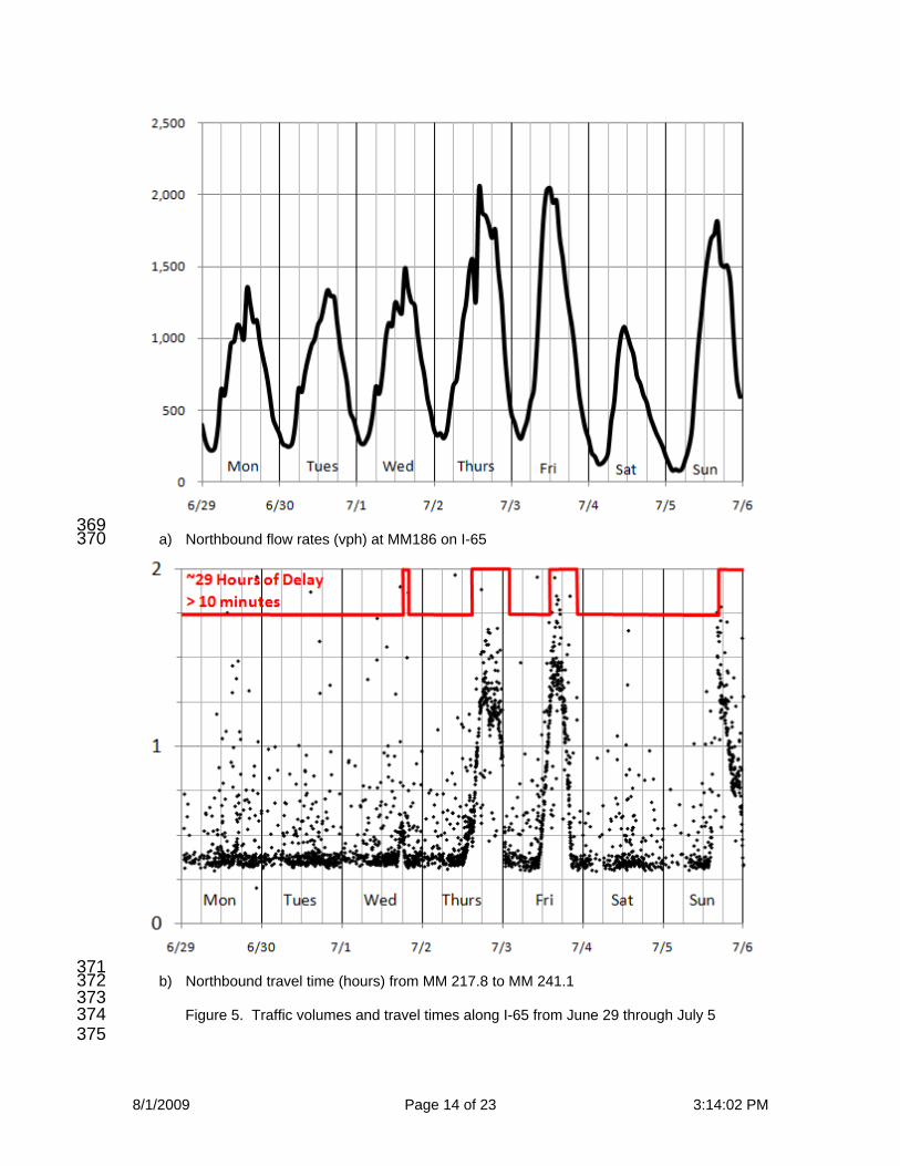
369 a) Northbound flow rates (vph) at MM186 on I-65 370

371 b) Northbound travel time (hours) from MM 217.8 to MM 241.1 372

373 Figure 5. Traffic volumes and travel times along I-65 from June 29 through July 5 374

375

8/1/2009 Page 15 of 23 3:14:02 PM

376

Figure 6. Percentage of week with delay > 10 minutes 377 378

379

8/1/2009 Page 16 of 23 3:14:02 PM

380 Figure 7. Effect of opening second southbound lane on southbound travel time (hours) 381

382 383

8/1/2009 Page 17 of 23 3:14:02 PM

384

385 a) Northbound hourly volumes at MM186 386

387 b) Northbound travel time (hours) from MM 217.8 to MM 241.1, May 1 to May 3 388 389

Figure 8. Effects of severe lane closing crash on travel times and traffic volumes, May 1 to May 3 390 391

8/1/2009 Page 18 of 23 3:14:02 PM

392

a) Northbound travel times, crash history, and queue trace

c) crash location map

b) Southbound travel times, crash history, and queue trace

Figure 9. June 29-July 5, 2009 393 394

8/1/2009 Page 19 of 23 3:14:02 PM

395

a) Northbound travel times, crash history, and queue trace

c) crash location map

b) Southbound travel times, crash history, and queue trace

Figure 10. June1 – June 7, 2009 396 397

8/1/2009 Page 20 of 23 3:14:02 PM

398

a) Northbound travel times, crash history, and queue trace

c) crash location map

b) Southbound travel times, crash history, and queue trace

Figure 11. July 20 – July 26, 2009 399 400

8/1/2009 Page 21 of 23 3:14:02 PM

401 a) Northbound volumes (vph) 402

403

404 b) Southbound volumes (vph) 405

406 Figure 12. Comparative hourly traffic volume counts at MM186 on I-65 407

408

8/1/2009 Page 22 of 23 3:14:02 PM

409 Figure 13. Travel Times Observed for probes between PDMS at MM218 and BP101 on US 241; 410

July 24-26,2009. 411 412

0

1

2

0:00 12:00 0:00 12:00 0:00 12:00 0:00

Friday Saturday Sunday

8/1/2009 Page 23 of 23 3:14:02 PM

Table 1. Construction Zone Lane Configuration Timeline 413 Date Range Northbound Southbound 5/4 to 5/22, MM228 to MM235 1 1 5/22 to 5/28 2 1 5/28 to 7/2 1 1 7/2 to 7/21 1 2 7/21 to 7/25, MM228 to MM238 1 1 7/25 on, MM233 to MM238 1 1

414 Table 2. Hours with delay > 10 minutes present and configuration of construction zone 415

Week Number

Date Range Northbound Hours of travel time data

Southbound Operation where delay >10 minutes

Lanes Open

Operation where delay >10 minutes

Lanes Open

hours % hours % Week 1 May 4-10 24 16.2 1 148 20 13.5 1 Week 2 May 11-17 11 11.3 1 97 9 9.3 1 Week 3 May 18-24 3 3.8 1-2 78 20 25.6 1 Week 4 May 25-31 22 16.5 2-1 133 12 9.0 1 Week 5 June 1-7 14 8.3 1 168 15 8.9 1 Week 6 June 8-14 18 10.7 1 168 15 8.9 1 Week 7 June 15-21 25 16.8 1 149 14 9.4 1 Week 8 June 22-28 18 12.6 1 143 8 5.6 1 Week 9 June 29-July 5 29 17.2 1 168 10 6.0 1-2 Week 10 July 6-July 12 35 20.8 1 168 0 0 2 Week 11 July 13-July 19 33 19.6 1 168 0 0 2 Week 12 July 20-July 26 40 29.4 1 136 27 19.9 2-1 416