Embed Size (px)
Citation preview
Real-Time Face Detection,Identification and Emotion Analysis
for Affective Human RobotInteraction
Anders Skibeli Rokkones
Thesis submitted for the degree ofMaster in Informatics: Robotics and Intelligent Systems
60 credits
Department of InformaticsFaculty of mathematics and natural sciences
UNIVERSITY OF OSLO
Autumn 2018


Real-Time Face Detection,Identification and Emotion
Analysis for Affective HumanRobot Interaction
Anders Skibeli Rokkones

c© 2018 Anders Skibeli Rokkones
Real-Time Face Detection, Identification and Emotion Analysis forAffective Human Robot Interaction
http://www.duo.uio.no/
Printed: Reprosentralen, University of Oslo

Abstract
In this thesis an approach for real-time face detection, identification and emo-tion recognition is presented, using robust face detectors and convolutionalneural networks (CNN). It is tested on a standard laptop computer withoutthe use of Graphical Processing Units (GPUs) and is to be implemented on anautonomous robot stationed in elderly users’ homes. In the real-time emotionrecognition pipeline it is shown that a small CNN trained on a personalizeddataset (images from a single user) is able to find faces, identify the user andclassify seven different emotions in real-time, contrary to related work thatprocesses data offline with fewer classes to predict. The use of a personalizeddataset reduces training time and increases robustness since a personalizedmodel is known to be more capable of learning person dependent features, assubstantiated in the results. Offline testing produces a top recognition rateof 98% and a real-time recognition rate of 83% of seven different expressions.Performance is expected to drop when introduced to a real-time testing en-vironment given more noise and variations. A comprehensive comparisonof existing pre-trained face detectors for fast classification is also presen-ted, showing that a Haar-cascade classifier, a Local-Binary-Pattern-cascadeclassifier and a Histogram-Oriented-Gradient classifier all pose as suitableoptions for real-time use.
In addition, offline experimentation with edge features in video combinedwith recurrent neural networks (RNN) and exploration of benefits and draw-backs of using sequential data for classifying facial expressions is presented.This includes the use of Kirsch masks and Local Directional Strength Patternas features presented as LDSP-RNN, achieving an average recognition rateof 73.6% on a fairly difficult dataset. It is compared with more traditionalimage classifiers such as CNN and Soft Vector Machines(SVM) for classi-fication where it is proven to outperform SVMs (72% mean accuracy) andproduce a more robust result than RNN with raw grayscale images as input(72.8% mean accuracy).
I
Acknowledgements
I am very grateful to Md. Zia Uddin and Jim Torresen for their guidanceand help during my work on this thesis, and the work they have performedprior to my thesis, giving me the opportunity to do a study within thisfield of healthcare and image analysis. Special thanks to my partner MariJunker and my parents Venke Skibeli and Erik Rokkones for support com-bined with writing and spelling corrections. Vetle Bu Solgaard, Bjoern-IvarTeigen and Martin Hovin deserve acknowledgments for letting me use themas test subjects along with support and encouragement; this applies to allmy co-students in the Robotics Lab at the Department of Informatics. Alsoa great appreciation to Epigram AI for letting me use their servers for someof the experiments.
II

List of Abbreviations
• CNN - Convolutional Neural Network
• RNN - Recurrent Neural Network
• SVM - Soft Vector Machine
• FCN - Fully Connected Network
• HRI - Human Robot Interaction
• RGB - Red, Green and Blue
• LDSP - Local Directional Strength Pattern
• LDP - Local Directional Pattern
• LBP - Local Binary Pattern
• HOG - Histogram Oriented Gradients
• LDRHP - Local Directional Rank Histogram Pattern
• LDSP-RNN - Local Directional Strength Pattern and RecurrentNeural Network
• RAW-IMAGE-RNN - Raw Grayscale Image and Recurrent NeuralNetwork
• CCE - Categorical Cross Entropy
• ReLU - Rectified Linear Units
• LDA - Linear Discriminant Analysis
• GAN - Generative Adversarial Network
• CK+ - Cohn-Kanade Extended Public Facial Expression Dataset
• AU - Action Unit
• IoU - Intersection over Union
• STD - Standard Deviation
• GPU - Graphical Processing Unit
• FPS - Frames Per Second
III

List of Figures
1.1 Information Flow . . . . . . . . . . . . . . . . . . . . . . . . . 2
2.1 Illustration of Possible Use . . . . . . . . . . . . . . . . . . . . 8
2.2 Kirsch Edge Masks . . . . . . . . . . . . . . . . . . . . . . . . 9
2.3 LDP vs. LBP . . . . . . . . . . . . . . . . . . . . . . . . . . . 10
2.4 LDSP vs. LDP . . . . . . . . . . . . . . . . . . . . . . . . . . 13
2.5 The Integral Image . . . . . . . . . . . . . . . . . . . . . . . . 14
2.6 Typical CNN Architecture . . . . . . . . . . . . . . . . . . . . 16
2.7 Illustration of an FCN . . . . . . . . . . . . . . . . . . . . . . 17
2.8 Dropout Network . . . . . . . . . . . . . . . . . . . . . . . . . 20
2.9 Dropout Improvement Plot . . . . . . . . . . . . . . . . . . . . 21
2.10 Data Augmentation . . . . . . . . . . . . . . . . . . . . . . . . 23
2.11 RNN Illustration . . . . . . . . . . . . . . . . . . . . . . . . . 25
2.12 Haar-like Feature Extraction . . . . . . . . . . . . . . . . . . . 28
2.13 CNN Architecture Used in DeepFace . . . . . . . . . . . . . . 28
2.14 Emotion Recognition in Images . . . . . . . . . . . . . . . . . 30
3.1 Emotion Images in Personalized Dataset . . . . . . . . . . . . 34
IV

3.2 Sequence Length Distribution in the CK+ Dataset . . . . . . 36
3.3 Class Distribution in Full CK+ Dataset . . . . . . . . . . . . 38
3.4 Class Distribution in Reduced CK+ Dataset . . . . . . . . . 38
3.5 Class Distribution in Personalized Dataset . . . . . . . . . . 38
3.6 Emotion Images in CK+ Dataset . . . . . . . . . . . . . . . . 39
4.1 Illustration of the System . . . . . . . . . . . . . . . . . . . . 42
4.2 RGB Channels . . . . . . . . . . . . . . . . . . . . . . . . . . 42
4.3 Image Scales Vs. Image Pyramid . . . . . . . . . . . . . . . . 46
4.4 Different minNeighbors Values . . . . . . . . . . . . . . . . . . 46
4.5 Illustration of Face Identification . . . . . . . . . . . . . . . . 48
4.6 Identification Model Architecture . . . . . . . . . . . . . . . . 48
4.7 Two-Class Model Architecture . . . . . . . . . . . . . . . . . . 50
4.8 Four- & Seven-Class Model Architecture . . . . . . . . . . . . 50
4.9 Face Detection Test Images . . . . . . . . . . . . . . . . . . . 54
4.10 Face Detector Comparison 1 . . . . . . . . . . . . . . . . . . . 55
4.11 Face Detector Comparison 2 . . . . . . . . . . . . . . . . . . . 55
4.12 Identification Model Training Progression . . . . . . . . . . . . 56
4.13 Identification Confusion Matrix . . . . . . . . . . . . . . . . . 57
4.14 Activation Map . . . . . . . . . . . . . . . . . . . . . . . . . . 59
4.15 Bar-Plot of Emotion Model Performances . . . . . . . . . . . . 60
4.16 Real-Time Emotion Predictions . . . . . . . . . . . . . . . . . 61
4.17 Confusion Matrix of Two-Class Emotion . . . . . . . . . . . . 62
V

4.18 Confusion Matrix of Four-Class Emotion . . . . . . . . . . . . 63
4.19 Confusion Matrix of Seven-Class Emotion . . . . . . . . . . . 64
5.1 Emotions Evolving Over Time . . . . . . . . . . . . . . . . . . 67
5.2 Class Distribution in Sequence Dataset . . . . . . . . . . . . . 67
5.3 Kirsch Mask Applied in 8 Directions . . . . . . . . . . . . . . 68
5.4 LDSP on 3x3 Pixel Neighborhood . . . . . . . . . . . . . . . . 69
5.5 3D-plot of Features . . . . . . . . . . . . . . . . . . . . . . . . 69
5.6 Input Image LDSP-RNN . . . . . . . . . . . . . . . . . . . . . 70
5.7 Best Training Run of LDSP-RNN . . . . . . . . . . . . . . . . 71
5.8 Bar-Plot of LDSP-RNN, RAW-IMAGE-RNN and SVM . . . . 73
5.9 RNN Confusion Matrices . . . . . . . . . . . . . . . . . . . . . 74
8.1 Training Progression - Two-Class Generalized Model . . . . . 94
8.2 Training Progression - Two-Class Personalized Model . . . . . 95
8.3 Training Progression - Four-Class Generalized Model . . . . . 96
8.4 Training Progression - Four-Class Personalized Model . . . . . 97
8.5 Training Progression - Seven-Class Generalized Model . . . . . 98
8.6 Training Progression - Seven-Class Personalized Model . . . . 99
VI

List of Tables
2.1 Categorical Cross Entropy vs. Classification Error . . . . . . . 22
3.1 The Three Datasets . . . . . . . . . . . . . . . . . . . . . . . . 35
3.2 Action Units . . . . . . . . . . . . . . . . . . . . . . . . . . . . 35
3.3 Emotion Description with AUs . . . . . . . . . . . . . . . . . . 37
4.1 Identification Classification Report . . . . . . . . . . . . . . . 56
4.2 Top 3 Results Two Emotions . . . . . . . . . . . . . . . . . . 59
4.3 Top 3 Results Four Emotions . . . . . . . . . . . . . . . . . . 59
4.4 Top 3 Results Seven Emotions . . . . . . . . . . . . . . . . . . 60
4.5 Classification Report Two Emotions . . . . . . . . . . . . . . . 62
4.6 Classification Report Four Emotions . . . . . . . . . . . . . . 63
4.7 Classification Report Seven Emotions . . . . . . . . . . . . . . 64
5.1 RNN Test Results . . . . . . . . . . . . . . . . . . . . . . . . . 73
VII

Contents
1 Introduction 1
1.1 Motivation . . . . . . . . . . . . . . . . . . . . . . . . . . . . . 2
1.2 Research Questions . . . . . . . . . . . . . . . . . . . . . . . . 3
1.3 Contributions . . . . . . . . . . . . . . . . . . . . . . . . . . . 4
1.4 Limitations . . . . . . . . . . . . . . . . . . . . . . . . . . . . 4
1.5 Structure of the Thesis . . . . . . . . . . . . . . . . . . . . . . 4
2 Background 7
2.1 Human Robot Interactions . . . . . . . . . . . . . . . . . . . . 8
2.2 Feature Extraction . . . . . . . . . . . . . . . . . . . . . . . . 9
2.2.1 Local Binary Pattern . . . . . . . . . . . . . . . . . . . 10
2.2.2 Local Directional Pattern . . . . . . . . . . . . . . . . 10
2.2.3 Local Directional Strength Pattern . . . . . . . . . . . 11
2.2.4 Haar-like Features . . . . . . . . . . . . . . . . . . . . 14
2.2.5 Histogram Oriented Gradients . . . . . . . . . . . . . . 14
2.3 Machine Learning for Image Analysis . . . . . . . . . . . . . . 15
2.3.1 Deep Learning . . . . . . . . . . . . . . . . . . . . . . . 15
VIII

2.3.2 Supervised Learning . . . . . . . . . . . . . . . . . . . 15
2.3.3 Classification . . . . . . . . . . . . . . . . . . . . . . . 17
2.3.4 Improving Convolutional Neural Networks . . . . . . . 18
2.3.5 Recurrent Neural Networks . . . . . . . . . . . . . . . 24
2.4 Face Detection . . . . . . . . . . . . . . . . . . . . . . . . . . 26
2.5 Identification . . . . . . . . . . . . . . . . . . . . . . . . . . . 28
2.6 Emotion Recognition . . . . . . . . . . . . . . . . . . . . . . . 29
3 Datasets 33
3.1 Emotion Datasets . . . . . . . . . . . . . . . . . . . . . . . . . 34
3.2 Identification Dataset . . . . . . . . . . . . . . . . . . . . . . . 39
4 Real-Time Emotion Recognition Pipeline 41
4.1 Approach . . . . . . . . . . . . . . . . . . . . . . . . . . . . . 42
4.1.1 Image Preprocessing . . . . . . . . . . . . . . . . . . . 42
4.1.2 Face Detection . . . . . . . . . . . . . . . . . . . . . . 44
4.1.3 Identification . . . . . . . . . . . . . . . . . . . . . . . 48
4.1.4 Emotion Recognition . . . . . . . . . . . . . . . . . . . 50
4.1.5 Evaluation of Real-Time Performance . . . . . . . . . . 52
4.2 Experiments & Results . . . . . . . . . . . . . . . . . . . . . . 54
4.2.1 Face Detection Results . . . . . . . . . . . . . . . . . . 54
4.2.2 Identification Results . . . . . . . . . . . . . . . . . . . 56
4.2.3 Emotion Recognition Results . . . . . . . . . . . . . . 57
4.3 Real-Time Evaluation . . . . . . . . . . . . . . . . . . . . . . 61
IX

5 Emotion Recognition Using Salient Features & RecurrentNeural Network in Video 65
5.1 Approach . . . . . . . . . . . . . . . . . . . . . . . . . . . . . 66
5.1.1 Making Sequence Dataset . . . . . . . . . . . . . . . . 66
5.1.2 Image Preprocessing . . . . . . . . . . . . . . . . . . . 67
5.2 Experiments & Results . . . . . . . . . . . . . . . . . . . . . . 69
5.2.1 Visualization of Features . . . . . . . . . . . . . . . . . 70
5.2.2 Training & Testing of Recurrent Neural Network Ap-proach . . . . . . . . . . . . . . . . . . . . . . . . . . . 71
5.2.3 Overview of Results . . . . . . . . . . . . . . . . . . . . 72
6 Discussion 75
6.1 Real-Time Emotion Recognition Pipeline . . . . . . . . . . . . 76
6.2 Emotion Recognition Using Salient Features & Recurrent NeuralNetwork in Videos . . . . . . . . . . . . . . . . . . . . . . . . 77
6.3 Ethical Dilemmas . . . . . . . . . . . . . . . . . . . . . . . . . 78
7 Conclusion 81
7.1 Real-Time Emotion Recognition Pipeline . . . . . . . . . . . . 82
7.1.1 Is it Possible to Process Facial Expressions at a Reas-onable Speed in Real-Time on a Standard Laptop Com-puter, Without the Help of a GPU? . . . . . . . . . . . 82
7.1.2 How Well Does a Personalized Model Perform Com-pared to a Generalized Model? . . . . . . . . . . . . . . 82
7.2 Emotion Recognition Using Salient Features & Recurrent NeuralNetwork in Video . . . . . . . . . . . . . . . . . . . . . . . . . 83
X

7.2.1 Can Oriented Gradient Features in Sequence CombinedWith an RNN Pose as an Alternative to Standard CNNs? 83
7.3 Dissemination . . . . . . . . . . . . . . . . . . . . . . . . . . . 83
7.4 Future Work . . . . . . . . . . . . . . . . . . . . . . . . . . . . 84
7.4.1 Real-Time Emotion Recognition System . . . . . . . . 84
7.4.2 Emotion Recognition Using Salient Features & Recur-rent Neural Network in Video . . . . . . . . . . . . . . 84
8 Appendix 93
8.1 Sensors, Software & Hardware . . . . . . . . . . . . . . . . . . 93
8.2 Emotion Recognition Training Plots . . . . . . . . . . . . . . . 94
8.2.1 Two Classes . . . . . . . . . . . . . . . . . . . . . . . . 94
8.2.2 Four Classes . . . . . . . . . . . . . . . . . . . . . . . . 96
8.2.3 Seven Classes . . . . . . . . . . . . . . . . . . . . . . . 98
XI

XII

Chapter 1
Introduction
1

Figure 1.1: Illustration of information flow through the system.
1.1 Motivation
The welfare of seniors has always been an essential part of society. By in-troducing new technology and applications, the people involved will be morecapable of managing their own life without too much help from the publicand private health sectors.
The Multimodal Elderly Care Systems (MECS project) aims at makingthe daily life more comfortable for the elderly and at the same time assisthealthcare personnel by providing additional information about the user.This thesis presents an approach for implementing an application which cananalyze emotions based on facial expressions of the user. This applicationwill be part of a mobile robot stationed in the users’ home where it also willperform other tasks like tracking movement, respiration, heart rate and ana-lyze other features associated with the user. If any anomalies are detected, aspecified response will be actioned to ensure that the users’ health is exposedto minimum risk, making this robot an autonomous safety alarm without theneed of attachments on the users themselves.
The primary goal of the thesis is to track the facial expression in real-time,something that may be computationally hard considering the hardware limit-
2
ations of the mobile robot. Different types of sensors can be combined to getthe optimal representation of the users’ face, where depth-, thermographic-and a regular RGB-camera pose as the best options for face tracking and fea-ture extraction. This may also introduce implications when it comes to pri-vacy in contrast to digital information (i.e., resolution, colour, etc.). Depth-and thermal cameras eliminate the privacy issues, but on the other hand,information that might be vital to obtain a proper classification will be lost.RGB-cameras provide more detailed images for analysis and are, therefore,the selected type of sensor utilized for training and testing of the presentedreal-time emotion analysis system.
1.2 Research Questions
To get a better understanding of the goal of the thesis, a series of threeresearch questions are defined and listed below. Each of the questions areconstructed so that the implementation and testing of chapters 4 and 5 arefocused on answering all of them in the best way possible.
1. Is it possible to process facial expressions at a reasonable speed in real-time on a standard laptop computer, without the help of a GPU?
2. How well does a personalized model perform compared to a generalizedmodel?
3. Can gradient oriented features in sequence combined with an RNN poseas an alternative to a standard CNN?
Figure 1.1 illustrates the flow of information through the pipeline. Focuswill be put into the emotion recognition part, considering it is the centralpart of the pipeline. Extensive research have been done on face detectionand identification in computer vision, leaving it hard to outperform existingimplementations, see sections 2.4 and 2.5. Comparing and discussing benefitsand drawbacks of existing implementations within these fields will help todecide on what would improve implementation of the pipeline the most.
3

1.3 Contributions
This section gives an overview of different contributions related to this work.
• The first contribution is an approach for real-time emotion classifica-tion with the use of small customized convolutional neural networkstrained on a personalized dataset for classifying seven different emo-tions which is presented in chapter 4. Included in this contribution isa comprehensive comparison of available pre-trained face detectors forreal-time applicability.
• In the following chapter (chapter 5) a combination of features in se-quences based on Kirsch edge detection and Local Directional StrengthPattern[1] and a recurrent neural network for emotion classification arepresented. The findings state that the LDSP-RNN approach producesa more stable and faster learning progression compared with a sequenceof raw image values.
1.4 Limitations
The public dataset, Cohn-Kanade+[2], used in some of the experiments hasshown deficiencies in the sense of a few miss-labeled samples and quite sig-nificant variations in class representations. This may reduce the ability fora CNN to learn the proper and generalized features required for a satisfyingoutcome. The problems related to this dataset limits the ability to generalizethe results presented in this thesis, but it presents a basis of which improve-ments are possible with the use of different datasets. Finding a new datasetfor experiments was considered to be work beyond the time frame associatedwith this thesis.
1.5 Structure of the Thesis
The majority of figures and tables are made specifically for this thesis. Ifnot, references to original figures or tables are provided in the captions ofthe respective figures or tables.
4

The thesis is structured to reflect the investigation of finding answers tothe research questions presented in section 1.2.
• Chapter 2 provides an overview of previous work related to each chapter,as well as techniques to help improve different deep learning architec-tures.
• Chapter 3 provides details about the datasets used in the experiments.
• Chapter 4 gives an approach for solving real-time face detection iden-tification and emotion recognition. Results are presented in section4.2.
• Chapter 5 explores a new way of analyzing facial expressions in videos,with the use of edge features and Local Directional Strength Pattern[1].
• Chapter 6 discusses the findings from chapter 4 and chapter 5.
• Chapter 7 provides a conclusion based on results from section 4.2 andsection 5.2, with answers to the research questions presented in 1.2,followed by future work in section 7.4.
5

6

Chapter 2
Background
7

2.1 Human Robot Interactions
Figure 2.1: Illustration of possible use
Humans have multiple ways of displaying their feelings and they differfrom person to person and culture to culture. Facial expressions have a sig-nificant place when it comes to communicating with one another and in someway remove the problem of misunderstandings when conveying a message.Digital communication is a big part of peoples lives, by the sending of e-mailsand chatting on social media. In this form of communication the limited abil-ity to put a facial expression behind the message can be troublesome. Thisis giving rise to problems which most likely would not be an issue if theconversation was held face to face. The introduction of emojis (small figuresof faces etc.) is enabling people to put a facial expression to their message,reducing the possibility of misunderstandings.
The same principle is relevant when it comes to communication betweenhumans and robots. With the advancements in technology, especially autonom-ous robots which interact with people, a good understanding between robotand human must be solved to enable further accomplishments. In the lasttwenty years machine learning and artificial intelligence have been the cen-ter of attention in computer science, resulting in a better environment forsignificant progress in the human-robot interaction domain. There are a lotof different aspects of this domain such as natural behavior, optimal pathand following basic norms. For autonomous robots and other assisting ap-plications, communication and understanding are essential factors to achieveresults surpassing pre-programmed responses to different scenarios. Humanfaces is a very complicated part of the body, consisting of multiple tiny
8

muscles that together can form a wide specter of expressions. By enablingrobots to use sensors like microphones and cameras, they will be given accessto the domain which also humans are dependent of to interpret one another.
2.2 Feature Extraction
Features, or data descriptors, is a big part of image analysis. Different meth-ods can be used to extract information within images beyond standard RGB-values (Red, Green, Blue) or grayscale values. In this section, an overviewis given of methods commonly used in face detection and emotion classifica-tion[1, 3, 4].
Kirsch Edge Detection
Kirsch edge detection is a mask that considers edge responses in all eight dir-ections around a single pixel. It is done by applying eight separate filters withvalues specifically to highlight edges oriented in the specified orientation[5].See figure 2.2.
Figure 2.2: Kirsch edge masks in eight directions[1].
9

2.2.1 Local Binary Pattern
Local Binary Pattern (LBP) was originally designed for texture descrip-tion. LBP assigns a binary label to every pixel of an image by comparingthe center pixel of a 3x3 neighborhood. If the surrounding pixels are largerthan the center pixel, it assigns 1, if smaller it assigns 0 [3]. The surroundingpixels, when considered in all 8 directions, produce an 8-bit representationof the area (3x3) as illustrated in figure 2.3. The operator is scanned acrossall pixels of the image, producing a binary representation for all the pixelsconverting this into a decimal representation. The result is a 1-dimensionalvector or histogram of the entire image providing a texture description of therespected image.
LBP (xc, yc) =7∑
n=0
s(in − ic)2n (2.1)
s(x) =
1, x ≥ 0
0, x < 0(2.2)
Figure 2.3: LDP vs. LBP on raw grayscale pixels.
2.2.2 Local Directional Pattern
Local Directional Pattern (LDP) compared to LBP, gives a better de-scription of the edges. This is due to the selection of the top n absolutevalues provided by the Kirsch mask (see section 2.2) in all eight directions
10
around the center pixel contrary to LBP that only checks if the surround-ing pixels are larger or smaller than the center pixel. LDP was proposedby Jabid, Kabir and Chae in 2010 as a local feature descriptor for objectrecognition[5]. In 2012 Jabid, Kabir and Chae proposed LDP as a featuredescriptor for face recognition as well, where they described the advantagesof using LDP instead of LBP. LDP provides more consistency in the presenceof noise since the edge response magnitude is more stable than pixel intens-ities[4]. As we can see in figure 2.3, LDP gives a more detailed descriptionof the edge response on a raw grayscale image than LBP.
LDP (xc, yc) =7∑
n=0
s(abs(in))2n (2.3)
s(x) =
1, topN(x) = True
0, topN(x) = False(2.4)
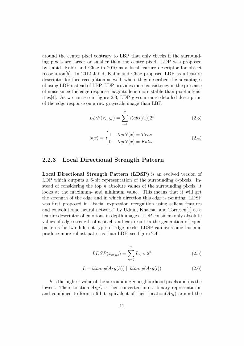
2.2.3 Local Directional Strength Pattern
Local Directional Strength Pattern (LDSP) is an evolved version ofLDP which outputs a 6-bit representation of the surrounding 8-pixels. In-stead of considering the top n absolute values of the surrounding pixels, itlooks at the maximum- and minimum value. This means that it will getthe strength of the edge and in which direction this edge is pointing. LDSPwas first proposed in “Facial expression recognition using salient featuresand convolutional neural network” by Uddin, Khaksar and Torresen[1] as afeature descriptor of emotions in depth images. LDP considers only absolutevalues of edge strength of a pixel, and can result in the generation of equalpatterns for two different types of edge pixels. LDSP can overcome this andproduce more robust patterns than LDP, see figure 2.4.
LDSP (xc, yc) =7∑
n=0
Ln × 2n (2.5)
L = binary(Arg(h)) || binary(Arg(l)) (2.6)
h is the highest value of the surrounding n neighborhood pixels and l is thelowest. Their location Arg() is then converted into a binary representationand combined to form a 6-bit equivalent of their location(Arg) around the
11

center pixel, where h is the three left bits and l is the three right bits,essentially making the highest neighboring pixel the most significant bits.
In figure 2.4 it is shown that LDSP is producing separate edge repres-entations for different edges, contrary to LDP that produces the same edgerepresentation for both edges. The figure is partially copied from Uddin,Khaksar and Torresen’s paper[1].
12

(a) First edge
(b) Second edge
Figure 2.4: LDSP vs. LDP on Kirsch edge values[1].
13

Figure 2.5: The integral image [8]
2.2.4 Haar-like Features
Haar-like features are digitally computed features used for object detection.At the beginning of digital image analysis, when considering working withonly RGB-values, it was considered hard to perform complex operations.Papageorgiou published a paper discussing the possibilities working withfeatures inspired by Haar-wavelets[6] instead of raw RGB-values [7]. Viola& Jones was inspired by this idea and proposed Haar-like features.
Haar-like features are based on dividing the image into regions and calcu-lating the sum of the pixels within these regions. By comparing the results ofneighboring regions it is possible to describe objects in the image. Haar-likefeatures are considered fast because of the use of the Intergral Image whichworks as a table of reference points equal to the size of the image making iteasy to calculate these features between two regions (see figure 2.5). Haar-likefeatures are used to train several weak classifiers and boosted with AdaBoostto form the Haar-cascade classifier as discussed in chapter 2 section 2.4.
2.2.5 Histogram Oriented Gradients
Histogram Oriented Gradients (HOG) features is represented as a singlefeature vector opposed to a set of feature vectors. It does so by computingthe gradients of a sub-window in the image and its orientations, dividing thedirections into 9 bins from 0 to 180 degrees with 20 intervals for each bin,
14

[0-20, 20-40, ..., 160-180]. The histogram is spiked where the prominentgradients are oriented. The calculated feature vector is then fed through aclassifier, usually a Soft Vector Machine(SVM) which decides if there is aface inside the sub-window or not.
Dalal and Triggs who first proposed the use of HOG-features in persondetection, argued that normalized Histogram Oriented Gradients performedexcellently compared with existing feature descriptors like Haar wavelets, andmanaged to prove that HOG reduced false positive rates by a magnitude re-lative to the best Haar-wavelet-based descriptors (i.e., Haar-like features)[9].
2.3 Machine Learning for Image Analysis
2.3.1 Deep Learning
The definition of deep learning varies somewhat between experts, but onething is certain; it is based on the knowledge of how the human brain workswith an intricate network of neurons cooperating to understand the worldaround it. An input vector, a hidden vector and an output vector are knownto many as a Multi-layered Perceptron. By expanding the number of hiddenlayers the network can solve more complex problems and to some extent geta deeper understanding of the underlying structure within the dataset. Thisis one of the reasons why it is called deep learning.
Deep learning models have substantially improved multiple domains withincomputer science such as speech recognition, object detection, object classi-fication and many other. Deep learning has made advances were problemsin the artificial intelligence community have resisted the best attempts atsolving them with traditional methods[10].
2.3.2 Supervised Learning
Supervised learning is a form of machine learning where the answers to eachdata point in the training set are known. This enables the model to getfamiliar with the problem in such a way that it can perform well on newunseen data. By knowing the correct answer to each input, the model canadjust itself to the point where the error between the predicted value and
15

actual value is minimized. This technique is widespread when it comes toclassifying images. CNNs are a form of supervised learning architecture andhas shown great performance in classifying images, object detection and asa feature extractor for further classification[1, 11, 12, 13, 14].
Convolutional Neural Networks for Feature Extraction
Figure 2.6: Typical CNN architecture[13].
”..manually acquiring some facial features from face images is relatively dif-ficult, while CNN could extract effective facial features automatically.” [14].
CNNs can find complex features in the raw image which manually wouldbe very difficult. By training the CNN on multiple images, it is able to extractcomplicated features and use them as descriptors for further classification.In two dimensional convolution, a filter of shape (NxN) slides over the imageresulting in a feature map representation of the input image. Each filterconsists typically of uniform initialized values. During training of a CNNthese values are changed through backpropogation[15] based on the gradientof the output error and ultimately they converge on the optimal filter valuesto find suitable features that represent the image. CNNs usually consist ofmultiple layers of convolution where each layer applies multiple numbers offilters where each filter is trained to find different features, for example edges,eyebrows, mouth, hair, color etc. The deeper the layer, the more complicatedthe features are[13, 14]. Between each convolution layer sub-sampling is used.This is to reduce the number of trainable parameters which easily can growquite large. Two different methods are customarily applied, Max Pooling andAverage Pooling.
16

”Pooling enhances the robustness to the variations of images. Such asrotation, noise and distortion. It also reduces the dimensions of the outputand reserves the notable features.”[14]
This is one of the reasons why CNNs is preferred when it comes to im-age processing. Figure 2.6 is a simple illustration of a convolutional neuralnetwork.
2.3.3 Classification
Figure 2.7: Simple illustration of a fully connected network
After good features have been extracted from the image, only a matter ofclassification remains. There are numerous different classification approachessuch as Soft Vector Machines, K-Nearest Neighbours, decision trees, etc.However, this section focus on probably the most commonly used classifyingmethod when it comes to deep learning. A fully connected network (FCN),also known as a multilayered perceptron, can be used for classification. Theinput to the FCN is a flattened vector representation of the extracted featuresfrom the images, as illustrated in figure 2.6. This vector is then fed throughthe FCN producing values at the output nodes. The number of output nodesis equal to the number of classes to predict, but for a binary classificationproblem only one node is typically used. Every node in the network is sub-jected to an activation function that forces a node to ”fire” if presented witha particular input which is inspired by how the brain works. The Sigmoidfunction is an example of such a function applied for a binary classificationproblem on the single output node. The Rectified Linear Units Function[16](ReLU) is more commonly used in the rest of the network because it avoidsgradient clipping of nodes with high values. As we can see in the functionbelow, high values for x will result in f(x) = 1 and the gradient is then equal
17

to 0 which does not contribute to the learning of the network.
f(x) =1
1− e(−x)(2.7)
The Sigmoid function ”squashes” the value of the output node to bebetween 0 and 1, making it a probabilistic function that states the probabilityof the input belonging to class A or class B.
class =
A, if f(x) ≥ 0.5
B, otherwise(2.8)
Between the layers of nodes are weighted connections called ”weights”.These weights are multiplied with the input to produce the next layer ofnodes, connecting each node in a layer to every node in the previous layer(see figure 2.7). After a forward pass through the network, the weights areadjusted with backpropagation based on the gradient of the error function(example Mean Squared Error[17]) at the output, and this process is repeateduntil the changes of the weights have converged and hopefully resulted ingood classification accuracy.
2.3.4 Improving Convolutional Neural Networks
Through the development of deep neural networks over the recent years dif-ferent techniques have been explored to stabilize weights with regularization,reduce overfitting and generalization of the network during training.
A standard convolutional neural network consists of N convolution layersfollowed by sub-sampling and an activation function with a fully connec-ted network at the output. The subsequent section gives a description oftechniques which have improved the performance of deep CNNs over the re-cent years and gives an understanding of why the architecture used in theexperiments was chosen.
18

Batch Normalization
Batch normalization was introduced by S. Ioffe and C. Szegedy in 2015 as anormalization layer in convolutional neural networks to reduce the numberof training steps by decreasing Internal Covariate Shift, a change in distribu-tions of internal nodes of a deep neural network during training[18]. Batchnormalization also has a positive influence on the gradient flow through thenetwork during backpropagation,
”... by reducing the dependence of gradients on the scale of the parametersor of their initial values..”
making it possible to use a higher learning rate with a reduced risk ofdivergence, as described in their paper[18].
This is done on a subset of training samples called mini-batches. Mini-batches or batches is useful in many ways. For example, when calculating thegradient of the loss on a mini-batch, you get an estimation of the gradientover the entire training set[18]. It also gives the advantage of parallel com-putations compared with single data point examples. Iofee and Szegedy’swork has inspired many adaptations of batch normalization, such as LayerNormalization[19] for use in recurrent neural networks and Adaptive BatchNormalization[20] to increase generalization of deep neural networks.
Mean and variance is calculated for each of the mini-batches and used tonormalize the activations. To avoid limiting what a layer represents, Ioffeand Szegedy introduced two parameters for each activation x(k) in a layer,γk and βk, to scale and shift the normalized values.
”... normalizing the inputs of a sigmoid would constrain them to the linearregime of the nonlinearity”[18].
These parameters are trained along with the weights and other trainableparameters in the network. For CNNs the parameters γk and βk are learnedfor each feature map in a layer instead of each activation.
In algorithm 1 the procedure to calculate a batch normalization for amini-batch is described as in Ioffe and Szegedy’s paper. Epsilon(ε) is a smallconstant that avoids the scenario of dividing by zero.
In their paper they also argue that with the use of Batch Normalizationthe need of Dropout is reduced, which leads us to the next section.
19

Algorithm 1 Batch Normalization Transform[18]
Input: Values of x over a mini-batch: B = x1...m; Parameters to betrained: γ, βOutput: yi = BNγ,β(xi)
µB ← 1m
∑mi=1 xi . mini-batch mean
σ2B ← 1m
∑mi=1(xi − µB)2 . mini-batch variance
xi ← xi−µB√σ2B+ε
. normalize
yi ← γxi + β ≡ BNγ,β(xi) . scale and shift
Dropout
Dropout was introduced by Srivastava et al. in 2014 as a regularization tech-nique to reduce overfitting in large deep neural networks[21]. Overfitting isthe result of deep neural networks that contain many hidden layers and iscapable of learning complex relationships between their inputs and outputs,learning sampling noise which is only present in the training set and notin the test set even though it is drawn from the same distribution[21]. Thismeans the network has become too familiar with the data it is training on res-ulting in poor performance when introduced with new unseen data. A layerof neurons will learn what to expect as output from its previous layer makingit vulnerable to small changes. To overcome this dropout was introduced.
Figure 2.8: Dropout illustration from Srivastava et al. paper [21]
Dropout is a term that refers to ”dropping” a unit or node either in hid-den or visible layers in a neural network. Essentially thinning the network, asshown in figure 2.8[21]. The dropout rate is the probability of a neuron “dy-
20

Figure 2.9: Dropout improvement plot from Srivastava et al. paper [21]
ing” in a specified layer, essentially producing a node-output equal to zero.This means that a neuron in the following layer will never learn with certaintywhat it will receive as input, drastically reducing overfitting. Dropout hasbecome a standard when implementing deep neural networks, underliningthe quite positive effect dropout has introduced to the deep learning domain.Figure 2.9 illustrates of how much networks without dropout is improvedwith the use of dropout. It is tested on different architectures where each issubjected to both cases.
Loss Functions
Categorical Cross Entropy(CCE) is one of the most commonly used loss func-tions for classification of multiple class labels and in many cases outperformother loss functions such as Squared Error [22, 23, 24].
CCE is a measurement of entropy between two probability distributions.Considering Softmax as the activation function on the output nodes and one-hot encoded labels, CEE would make a preferable choice as loss function.
This function describes the mean cross entropy with batch m:
L =1
m
m∑i
−yi × log(yi) (2.9)
21

Where y is the class labels represented as a one-hot encoded matrix andy is the predicted, Softmax-activated, matrix.
Softmax Labels Hit?LossCCE
ClassError
0.4 0.3 0.3 1 0 0 yesA 0.3 0.5 0.2 0 1 0 yes 1.07 0.33
0.6 0.2 0.2 0 0 1 no0.8 0.1 0.1 1 0 0 yes
B 0.05 0.9 0.05 0 1 0 yes 0.51 0.330.6 0.1 0.3 0 0 1 no
Table 2.1: Categorical Cross Entropy vs. Classification Error
Comparing CCE to a simple classification error function that checkswhether the correct class is predicted or not, the benefits of using CCE as aloss function becomes apparent. In table 2.1 we can see that CCE is muchmore descriptive of how well the softmax predictions match the labels. Out-put A produces the same correct predictions as output B, but the probabilityof the predicted class is not as prominent as in output B. The classificationerror is 0.33 for each of the cases resulting in the same amount of weightadjustment during a backpropagation, contrary to CCE which will take intoconsideration the differences between these distributions.
Optimizer
Optimizers are used to navigate the solution space of a function with thegoal of finding the global and optimal solution for that function.
In machine learning we try to minimize the loss function as much as pos-sible without overfitting during training. This is done with weight adjust-ment through backpropagation where an optimizer tries to steer the gradientof the loss function in a direction towards the global optimum, meaning thatit attempts to find the correct weight values between each layer in a networkto produce a result closest to the correct answer. The derivative of the lossfunction gives the optimizer an estimation in which direction it is moving re-lative to the optimal solution. It can encounter false optimal solutions calledlocal optima that can seem like a good solution, but in the bigger picture pro-duce a sub-optimal result. Optimizers are prone to get stuck in local optimaand different optimizers have been developed over the years trying to escape
22

these and reaching the global optimum as fast as possible. Techniques suchas momentum have been added to increase the chance of escaping.
Adam is an optimization algorithm proposed by Kingma and Lei Bain 2015[25]. The name Adam is derived from Adaptive Moment estimationand is based on the best qualities from two popular methods: RMSProp[26]and AdaGrad [27]. Kingma and Lei Ba concluded that Adam is a suitablemethod for large datasets or high dimensional parameter spaces. It is robust,easy to implement and an efficient optimization algorithm with little memoryrequirements[25]. Taking this into consideration Adam is a much-suited op-timizer to be used in this thesis.
Data Augmentation
Figure 2.10: Random rotation of +/- 10 and horizontal flipping.
Convolutional Neural Networks are commonly known to require a sub-stantial amount of training data. In the cases of sparse training sets with lowvariance, CNNs can easily overfit during training. A solution to this problemcan be to generate more data either artificially or by manually labeling newdata.
A second option can be to augment the existing data. The idea is toapply a random set of operations on the input images, such as rotation, ho-rizontal/vertical flipping, adding noise and rescaling. In the perception ofthe network it will get new training data for every new augmentation, es-sentially increasing the number of training samples and reducing overfitting.Perez and Wang explored The Effectiveness of Data Augmentation in ImageClassification using Deep Learning [28], testing different traditional augment-ation techniques as mentioned above, but also experimented with the use ofGenerative Adversarial Networks(GAN[29]) to generate new images. Theyconcluded with increased classification accuracy and a reduction of overfittingwith the use of traditional augmentation techniques.
23

In this thesis, more traditional augmentation methods are applied suchas a small degree of random rotation and random horizontal flipping of theimages. See figure 2.10.
2.3.5 Recurrent Neural Networks
Recurrent Neural Networks (RNN) are designed to handle sequences of datamaking classifications based on data point occurrences over time. Examplesof this can be text (sentences) or videos. By looking at how specific obser-vations develop over time it can predict the next step in a sequence. RNNshave resulted in many impressive results such as Zach Thoutt’s attempt totrain an RNN on the famous book series Game of Thrones written by GeorgeR.R. Martin, enabling it to write the ”next” book[30]. The result did notmake much sense in most cases, but it is apparent that the network was ableto learn essential writing techniques like quotes, paragraphs and generallyproper spelling, but also relationships between the different characters in thebook.
RNNs process a sample for each time step from the sequence of one-dimensional vectors. The hidden state is computed based on the previoushidden state(ht−1) at time(t-1) and the current input(xt) at time(t):
ht = σh(Wixt +Whht−1) (2.10)
The input and previously hidden state is multiplied with Wi, which isthe input weight matrix, and Wh which is the recurrent matrix. The sum ofthese two results is then fed through a hidden activation function σh, usuallyTanH-activation:
tanh(x) =sinh(x)
cosh(x)=ex − e−x
ex + e−x=
1− e−2x
1 + e−2x(2.11)
24

−4 −2 2 4
−1
−0.5
0.5
1
which compared to sigmoid-activation extends the ”activation range”from -1 to 1.
yt = σy(Woht) (2.12)
For every time step an output is computed (yt), where Wo is the outputmatrix and σy the output activation function. This means that we can getthe output at the time step that we prefer as illustrated in figure 2.11.
Figure 2.11: Simple RNN illustration, based on figure from[31]
”.. an RNN has the ability to learn to detect an event, such as the presenceof a particular expression, irrespective of the time, at which it occurs in asequence.”[31]
In Ebrahimi Kahou et al.’s paper[31] they present an approach that in-cludes using an RNN to classify facial expressions in videos. Their work is
25

very much related to the proposed implementation described in chapter 5where the classification of facial expressions is done with recurrent neuralnetworks. Contrary to the implementation in chapter 5 they make use of aCNN to extract features, whereas the approach explained in this thesis ex-periments with Local Directional Strength Patterns [1] as features and RNNcombined with FCN as classification.
In Ebrahimi Kahou et al.’s paper they use a variant of RNN called IRNN.Usually an RNN utilizes TanH as activation function, but with the problemof exploding and vanishing gradients, which is a problem when handling longsequences, an alternative was proposed were Rectified Linear Units was usedinstead and with a recurrent matrix that was initialized with scaled variationsof the identity matrix, as described in [31, 32].
2.4 Face Detection
The first problem to be solved is to find the face in real-time, which is com-monly the first stage in almost every face related computer vision system,and the aim is to get a high positive detection rate even with challengingbackgrounds. In this section an overview of previous work related to facedetection is presented.
Face detection can be quite tricky considering the diversity of faces inthe world including local variations such as light conditions, orientation, etc.Despite this, significant progress has been made in recent years[33]. A fastalgorithm for face detection is needed in the proposed implementation inthis thesis due to the robots limited computational power. Viola and Jonesproposed a suitable algorithm for fast face detection in “Robust real-timeface detection”[8]. In their paper they introduce a model based on Haar-like features (see section 2.2.4, and figure 2.12) in a cascade classifier. If aproposed segment fails on one of the weak classifiers, it is discarded. Thisensures a high classification accuracy, and even though the number of sub-windows and features are immense, the detector calculates this very quickly.Though Haar-like features are suitable for real-time face detection, it worksbest when it comes to well lit frontal faces as stated in Ranjan, Patel andChellappa’s paper[34]:
26

”It has been shown that in unconstrained face detection, features like HOGor Haar wavelets do not capture the discriminative facial information at dif-ferent illumination variations or poses.”
However, the cascade method can be used in combination with differentfeatures like Local Binary Patterns or automatically accumulated featuresfrom a convolutional neural net, like Li et al. did in their paper [35]. Sincethe hardware on the robot is limited, deep CNNs pose a threat when itcomes to speed, leaving traditional methods such as cascade classifiers withHaar-features[8], local binary patterns or HOG-features as excellent options.
Rajan, Patelan, and Chellappa proposed a quite inventive approach tocombine task solving in a CNN [34]. They called it HyperFace, and it is aCNN that predicts face detection, landmark localization, pose estimation andgender recognition. The idea is based on the knowledge of what informationeach layer of a CNN is able to extract. The first layers usually detect roughfeatures like corners, edges, etc. and is suitable for localization and poseestimation. The deeper layers have more fine-tuned and specific features;these can be used for gender recognition and face detection. This work canbe applied to my application where face detection, identification and emotionrecognition is constrained to a single CNN, but it is likely not suitable forreal-time classification as stated earlier.
The proposed emotion recognition system only needs to find the face once.Rather than scanning the whole image searching for a face for each framecaptured by the camera it can look in regions close to the location of wherethe face was in the previous frame. This can be done with face tracking. Thepython library dlib[36] has a function called correlation tracker which tracksa given object in an image stream by guessing the next position of the objectin the next frame based on previous frames and a confidence score. This willprobably increase the speed since it only needs to scan the whole frame untilit finds the correct face, optimally only once each time the user is enteringthe field of vision.
A similar tracking alternative is implemented by OpenCV [37], calledKernelized Correlation Filters (KCF). KCF is a tracking method that ex-ploits circulant matrix properties to enhance processing speed. As writtenin OpenCV’s reference guide: This tracking method is an implementationof Henriques, Caseiro, Martins, Batista Exploiting the Circulant Structure ofTracking-by-Detection with Kernels [38] which then is extended to KCF withcolor features[39].
27

Figure 2.12: Haar-like feature extraction[40]
When the face is extracted, it leads to the next step in the pipeline,identification. This is to ensure that only the users face is analyzed, and sothe privacy of visitors and other people is respected.
2.5 Identification
Figure 2.13: Identification CNN architecture used in DeepFace[41]
In this section, previous work related to the identification of human facesby the use of the different models available is presented. Also in this stage,speed is essential as well as accuracy. By identifying the correct face quicklythe system/pipeline will be able to start analyzing the facial expression andmake a classification.
Face identification is a technology with an increasing use on differentdevices ranging from unlocking smart-phones and payment verification tosecurity measures when entering restricted areas. When it comes to mobiledevices, the identification models are expected to be highly accurate, but alsosmall and fast. Most CNN models that predict with high accuracy are verydeep and is reliant on powerful hardware to make the calculations within areasonable time. Chen et al. proposed efficient CNNs for accurate real-timeface verification on mobile devices[42]. The number of trainable parametersin a CNN is one of the factors that consume processing time. A fairly big
28

architecture can easily contain multiple millions of parameters. VGG[43] isan example of this with 138 million parameters. The MobileFaceNets[42] hasmanaged to reduce the number to less than 1 million significantly increasingthe speed with no cost in accuracy.
As described earlier, CNNs are one of the best feature extractors of im-ages. A method utilizing this is described in Guo, Chen and Li’s paper wherethey propose a way to enhance classification rates by the use of CNN andSupport Vector Machine(SVM). In their paper they use the CNN to extractfeatures and the SVM to do the classification. They chose the SVM as analternative to a fully connected network;
”..we chose SVM to recognize faces as its excellent performance in solvinglinear inseparable problem. [14].
Support Vector Machine is a machine learning classifier which uses sup-port vectors to define a decision line that separates data based on theirfeatures. As Guo, Chen and Li says in their paper;
” For linear inseparable problem, SVM maps input in low dimensions intohigher dimension feature space that makes separation easier.”[14]
They proved that the combination of CNN + SVM improved the averageclassification rate of 0.615 % on their test data compared to a standard CNNwith a fully connected classifier. This approach is a strong candidate, butsince the identification task related to this system is a binary classificationproblem (user/not user), a simple CNN should suffice.
2.6 Emotion Recognition
Today, facial expression recognition is a very researched field in computervision [1, 11, 44, 45]. Despite this it is proven hard to implement an auto-matic model to perform this task [11, 46]. To actively monitor the facialexpression frame by frame and make predictions can be quite computation-ally difficult. The best results within facial expression classification are donewith comprehensive feature extractions combined with deep neural networksor CNNs as described in Uddin, Khaksar and Torresen’s paper[1].
Offline training and testing of models can give good results, but if presen-ted with live image streams it may cause poor performance. In recent years,
29

Figure 2.14: Emotion recognition in images[2]
approaches involving CNNs have shown the best advancements in the com-puter vision field [11, 12, 14, 1, 35, 42]. Exploiting the ability of featureextraction that CNNs possess and perhaps combining them with other fea-tures to get better classification is proven favorable in many cases[1, 11].
In Uddin, Khaksar and Torresen’s paper they used an approach withLocal Directional Rank Histogram Pattern (LDRHP) in combination withLocal Directional Strength Pattern (LDSP) as features for classifying emo-tions in depth images. LDSP calculates relative edge response values of apixel in different directions based on the outputs from a Kirsch edge detectorsince it considers edges in all eighth directions[5] (see section 2.2). This com-bination where LDSP is augmented with LDRHP is presented as LDRHP ||LDSP, and it generates a histogram were dimensions are reduced with ker-nel principal component analysis and general discriminant analysis to betterrepresent the features in the images. A CNN is then trained on these fea-tures, and the idea is that the network is more capable of learning salientfeatures (important features) which again results in better classification. Es-sentially this approach is based on directions of the gradients in the imagesand classified with a CNN. By replacing the CNN with an RNN it is possibleto answer the question about gradient based descriptors combined with anRNN.
30

Uddin, Khaksar and Torresen’s model[1] was trained on 6 classes withdepth images expressing these emotions:
1. Anger
2. Happiness
3. Sadness
4. Neutral
5. Surprise
6. Disgust
Contempt and fear is the seventh and eighth facial expressions as describedin the Cohn-Kanade+ dataset documentation[2], but was not used in theapproach described above.
In Alizadeh and Fazel’s paper[11], they describe an approach solely basedon a CNN architecture and fully connected layers for classification on anemotion recognition dataset of grayscale images from Kaggle[47]. They ap-plied different techniques to reduce overfitting on the training set such asdropout (see section 2.3.4), batch normalization (see section 2.3.4) and L2-regularization, but their best results did not surpass 60% accuracy on thetest set compared to Uddin, Khaksar and Torresen’s approach that managedto achieve a recognition rate of 97.08%. Note that these two models weretrained on different datasets where [47] may contain more variations in light,orientation etc. than [1] that trained on their own depth image dataset.
31

32

Chapter 3
Datasets
In this chapter, a brief overview of the applied datasets is presented. Com-paring differences and drawbacks related to both a personalized dataset anda public dataset.
33

(a) Anger (b) Contempt (c) Disgust (d) Fear
(e) Happiness (f) Sadness (g) Surprise
Figure 3.1: Images of emotions in personalized dataset.
3.1 Emotion Datasets
For this thesis personalized datasets of myself, as the user, will be applied fortraining and testing of the real-time classification system. This is to enableexploration of the CNNs ability to enhance classification rate and comparethe findings with the use of public datasets like the CK+ facial expressiondataset [2], highlighting the benefits of using a personalized dataset contraryto a public dataset.
Three data sets was constructed with varying number of facial expres-sions, see table 3.1.
Every result is compared with the Cohn-Kanade+ dataset as benchmark[2]. The four class personalized dataset will be a bit different than the CK+equivalent; this is due to the lack of degrees of happiness in the CK+ dataset.Instead, degrees of sadness/anger will be used as the CK+ alternative. Onecan argue that feature wise, happy/glad is the inverted version of angry/sad.
Cohn-Kanade+ dataset is a public dataset containing sequences ofvarying length with eight different expressions as listed in table 3.1. Theeighth expression is Neutral, but has no sequence dedicated to illustrating
34

Two classes Four classes Seven classesGlad Sadness AngerNot glad Neutral Disgust
Glad ContemptHappy Fear
HappySadnessSurprise
Table 3.1: The three different dataset with their respective classes
this expression. It is counted as an expression in the CK+ dataset dueto every sequence containing a neutral state before entering full emotiondisplay, meaning each participant displays an expression from neutral topeak expression.
When constructing an emotion, certain features must be present in theface called Action Units - AU where 30 different actions are labeled, see table3.2 and 3.3. These action units, or muscle contractions, for categorizingfacial expressions are described in Manual For The Facial Action CodingSystem[48] also known as FACS, written by P. Eckman and W. Friesen.
AU Name N AU Name N AU Name N1 Inner Brow Raiser 173 13 Cheek Puller 2 25 Lips Part 2872 Outer Brow Raiser 116 14 Dimpler 29 26 Jaw Drop 484 Brow Lowerer 191 15 Lip Corner Depressor 89 27 Mouth Stretch 815 Upper Lip Raiser 102 16 Lower Lip Depressor 24 28 Lip Suck 16 Cheek Raiser 122 17 Chin Raiser 196 29 Jaw Thrust 17 Lid Tightener 119 18 Lip Puckerer 9 31 Jaw Clencher 39 Nose Wrinkler 74 20 Lip Stretcher 77 34 Cheek Puff 110 Upper Lip Raiser 21 21 Neck Tightener 3 38 Nostril Dilator 2911 Nasolabial Deepener 33 23 Lip Tightener 59 39 Nostril Compressor 1612 Lip Corner Puller 111 24 Lip Pressor 57 43 Eyes Closed 9
Table 3.2: Action Units for Facial Expressions[2]
Regarding generating a personalized dataset, a few things have tobe considered. A person dependent emotion classifier has to get familiarwith the unique expression of its user, meaning that features which make aperson dependent emotion unique have to be present in the images providedto the classifier, at the same time trying to include the proper action unitsdescribing that emotion in a general view. This is to enhance the ability tomake a reasonable comparison of results between the Cohn-Kanade+ datasetand the personalized dataset.
35

(a) Anger
(b) Contempt (c) Disgust
(d) Fear (e) Happiness
(f) Sadness (g) Surprise
Figure 3.2: Sequence length distribution in the CK+ dataset
36

Emotion CriteriaAngry AU23 and AU24 must be present in the AU combinationDisgust Either AU9 or AU10 must be presentFear AU combination of AU1+2+4 must be presentHappy AU12 must be presentSadness Either AU1+4+15 or 11 must be present. An exception is AU6+15Surprise Either AU1+2 or 5 must be presentContempt AU14 must be present (either unilateral or bilateral)
Table 3.3: Emotion Description with Action Units[2]
In figure 3.3 the class distribution of the whole CK+ dataset is shown,consisting of 5880 separate grayscale images divided over seven classes. Aswe can see, there is not an equal distribution of images between each expres-sion. The difference between Happy and Contempt is approximately 1100images, this means that Happiness is 550% greater than Contempt whichis only 3,4% of the entire dataset and is shown in figure 3.3. This skew inthe distribution may be a problem when training the model for classifica-tion. One explanation could be that there are more neutral images in theclasses with higher representation. In the CK+ documentation[2] it is saidthe sequences vary in length from 10 to 60 frames, but in reality, it is 5 to 70frames. By looking at the sequence length distributions for each expressionin figures 3.2a-g, the classes with the lowest number of images representingeach emotion contain the long sequences. By comparing figure 3.3 and figure3.4, which is the reduced dataset with only peak emotion displays, the dis-tribution between the classes remain the same. This indicates that neutralimages in each sequence do not interrupt with the amount of actual emotiondisplays for each class.
The CK+ dataset has to be reduced in size since we are only interestedin the peak expressions from each sequence when training a CNN on thoseimages, making the total size of both the CK+ dataset and the personalizeddataset reasonably similar.
Figure 3.5 presents the class distribution of the personalized dataset con-taining images of one user. As mentioned earlier, expression criteria - ActionUnits - and person independent features of the individual expression, is at-tempted to co-exist in every emotion display.
A personal judgment was made when deciding which emotion that con-tains the most subtle features. Contempt stood out as one of those expres-
37

Figure 3.3: Class distribution in full CK+ dataset.
Figure 3.4: Class distribution in reduced CK+ dataset.
Figure 3.5: Class distribution in personalized dataset.
38

sions, including sadness. In light of these assumptions an increase in thenumber of images representing those expressions was made, while keepingalmost the same ratio between the other classes. This difference might havean impact on how well the models presented can learn from them, but it willbecome clear it is not a significant contributor to the contrast between theresults of the personalized and generalized model (i.e., model trained on apublic dataset).
(a) Anger (b) Contempt (c) Disgust (d) Fear (e) Happiness
(f) Sadness (g) Surprise
Figure 3.6: Images of emotions in Cohn-Kanade+ dataset[2].
3.2 Identification Dataset
Separating two classes using deep learning is commonly considered to be aless complex task. With the need of a relatively small dataset or at leastfewer data representations of each class, a reduction in the number of hiddenlayers in the deep learning model is possible, which again results in a decreasein training time.
The two classes represented in this dataset is User/Not-User, with roughlythe same amount of images in each class. The Not-User class is a set of imagesof fellow students which have agreed to participate as test subjects and thattheir data can be used for training of an identification model.
39

40

Chapter 4
Real-Time EmotionRecognition Pipeline
In this chapter the proposed approach for constructing a functional pipelineof Face Detection - Identification - Emotion Recognition for real-time applic-ability is presented, visiting different complications and obstacles and thesolutions applied to overcome these.
41
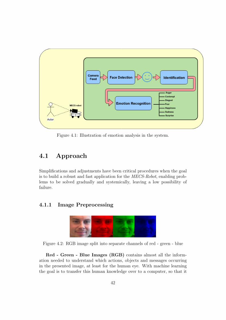
Figure 4.1: Illustration of emotion analysis in the system.
4.1 Approach
Simplifications and adjustments have been critical procedures when the goalis to build a robust and fast application for the MECS-Robot, enabling prob-lems to be solved gradually and systemically, leaving a low possibility offailure.
4.1.1 Image Preprocessing
Figure 4.2: RGB image split into separate channels of red - green - blue
Red - Green - Blue Images (RGB) contains almost all the inform-ation needed to understand which actions, objects and messages occurringin the presented image, at least for the human eye. With machine learningthe goal is to transfer this human knowledge over to a computer, so that it
42

can perform tasks that previously only humans could do. An RGB image isrepresented as a three-layered matrix with shape (width x height x channels),where the channels are Red, Green and Blue ranging in value from 0 to 255.In an image with pixel values that are all red, the channel values will therebylook like this [255, 0, 0]. [255, 255, 255] = white, [0, 0, 0] = black.
Image preprocessing is a term used for techniques that are appliedbefore any calculations or processing is done. An example of this can befeature extraction, like Local Directional Pattern (see section 2.2), filteringe.g. Kirsch edge detection and also image value normalization.
Normalization aims at smoothing out the data, removing or mutingextreme values called outliers. Max-Min Normalization is a popular nor-malization method and is used in this approach. Below is the function thatcalculates the normalized pixel values zi which is being used as a normaliz-ing function on the images before they are presented as input to the CNNsdescribed in the identification and emotion recognition experiments, section4.2.
zi =xi −min(x)
max(x)−min(x)
x = (x1, x2, ..., xn) is the data points or pixels in this case. The min-imum value of x is subtracted from xi and then divided by the differencebetween the maximum and the minimum value of x. The result is z whereall the pixel values are ”squashed” between 0 and 1. OpenCV’s normalizeimplementation[37] was used for preprocessing of the image datasets.
Neural networks modifies the weights so that the output value matchesthe target or class label. With seven classes, the value to be predicted isranging from 0 to 6 where these values are arranged in a way that the correctclass corresponds to its location in a list, called one-hot encoding. Withthe example below, we have four images with class labels 4, 2, 5 and 3respectively. In one-hot encoding, it will be converted into a matrix wherea single row represents one sample and the location where this row equals 1corresponds to the class label of that same sample.
[4, 2, 5, 3] =
0 0 0 0 1 0 00 0 1 0 0 0 00 0 0 0 0 1 00 0 0 1 0 0 0
43

With the labels represented in this way, we can use Softmax [49] activationat the output nodes. Softmax is a logistic activation function similar toSigmoid, but it can handle multiple outputs. It takes the output and rescalesit between 0 and 1, turning it into a probabilistic representation where thenode closest to 1 is the most likely class prediction of that input.
In equation 4.1 an example image of class 4 is passed through the deepneural network. It produces a set of example output values represented inthe first vector with length equal to 7.
1.02.00.53.05.00.20.1
⇒ S(yi) =
eyi∑j e
yj⇒
0.0140.0400.0090.1100.8120.0070.006
(4.1)
y is the predicted value at each output node, called logits. After applyingSoftmax, the predicted class, as we can see in the far right vector, is closest to1 in position 4. Using this new vector, we can calculate the loss by comparingit with the one-hot encoded class labels illustrated above. Since it is thecorrect class, the loss will be smaller compared to a different prediction. Thecalculated error, or loss, depends on which loss function is used. See section2.3.4 about Categorical Cross Entropy.
This leads us back to the normalization part. Instead of the neural net-work generating weight matrices that downscale the pixel values, we applynormalization before we train the network. This will result in better adjust-ments of weights during training, and the need of a normalization layer inthe CNN is reduced, but for the models classifying 4 or more emotions, anormalization layer has been used in the first layer. See section 2.3.4 aboutBatch Normalization and figure 4.8.
4.1.2 Face Detection
It exists many face detection algorithms in public python-libraries such asOpenCV[37] and dlib[36]. One criterion when it comes to choosing a facedetector is speed, but also accuracy. Therefore a comparison between the ex-
44

isting methods available from these libraries is conducted. This is to ensurethat the face detector used provided fast calculations and high accuracy.When measuring accuracy, false-positives are ignored and not counted al-though it detects a positive face. Considering this, subsequent stages in thepipeline can focus on actual faces, hence saving time and making the entireanalysis faster.
Scale Factor
Viola & Jones’ face detector scans the input image at many different scales,like most face detection systems. An image can contain numerous faces loc-ated at various distances as displayed in figure 4.9a and 4.9b. The scalefactor ensures that faces close- and far from the camera has a higher possib-ility of detection. Conventionally a scale factor of 1.25 is used to generatea pyramid of 12 images where each image is 1.25 times smaller than theprevious one. Processing every layer of images in this pyramid and applyingfeatures at each scale is proven to be quite a comprehensive operation[8].Viola & Jones’s face detector scans the input image at 12 scales. Starting atthe base dimensions of 24x24 to detect faces, for each iteration the slidingwindow increases by a factor of 1.25[8]. With a cascade classifier, eliminatingregions and applying features can be done at any scale and location in a fewoperations, dramatically speeding up the face detection process.
scaleFactor is a parameter that has to be passed to OpenCV’s detect-MultiScale[37]. It is important to test for different scales to find the suitablevalue which ensures a good classification and processing speed. Low scalefactors are equal to a small difference in size of the sliding window for eachiteration, resulting in a slower, but more accurate classification. A high scalefactor will do the opposite. It requires fewer iterations due to more rapidincrease in sliding window size, but with a higher chance of incorrect classi-fication. An illustration of how the sliding window increases are depicted infigure 4.3a, and in figure 4.3b the conventional image pyramid.
Minimum Neighbors
When using a set of features to decide if an object is present or not, it isalmost unavoidable to encounter false-positive classifications, meaning thatthe object has been classified to something it is not. An example of this
45

(a) Different Image Scales (b) Image Pyramid [50]
Figure 4.3: Image Scales Vs. Image Pyramid
can be finding faces in an image with no faces. Somewhere in the fore- orbackground at a specific scale and location, the features describe what isknown to the classifiers as a face and will mark the region accordingly. Thiscan and will happen if we do not try to dim the sensitivity of the classifier.
(a) Example of minNeighbors=0 [51] (b) Example of minNeighbors=3 [51]
Figure 4.4: Different minNeighbors values.
minNeighbors is the second key parameter to be passed to OpenCV’sdetectMultiScale[37]. It specifies how many neighbors or overlapping bound-ing boxes that are required for a face to be accepted. In figure 4.4a minNeigh-bors is set to 0. As we can see, the number of detections is overwhelmingconsidering that it finds faces in trees, rocks, ground, etc. because featuresdescribing these areas are similar to the features of a face. By increasing thethreshold of the minimum number of neighbors, we eliminate single ”weak”classifications and focus on those areas which have stronger features. In fig-ure 4.4b minNeighbors is set to be 3, and the true faces in the image havebeen found and it ignores false-positives. Again, finding the right number ofneighbors is also important when it comes to choosing a good face detector.
46

Selecting a number which is too low, will result in many false-positives. Onthe other hand, selecting too many and it might overlook areas where thereis a face.
Face Descriptor Comparison
The pre-trained face detectors used in this comparison is:
1. Haar-cascade classifier
2. LBP-cascade classifier
3. dlib’s get frontal face detector - returns a face detector based on histo-gram of oriented gradients (HOG-features)
4. Other pre-trained face detectors available in OpenCV for better com-parison, that are present in figures 4.10 and 4.11.
Above is the list containing the different face detectors used for compar-ison in section 4.2.1 with the aim of selecting a face detector best suited forreal-time applicability in the presented emotion recognition system.
The first pre-trained detector to be tested is Haar-cascade classifier whichis trained on Haar-like features as described in section 2.2.4 and 2.4.
The second classifier is also a cascade classifier, but it is trained on LocalBinary Patterns(see section 2.2.1) instead of Haar-like features. Both cascadeclassifiers are tested on different scales and minimum neighbors to find thebest-suited parameter settings for good face localization and classification,see section 4.1.2 and 4.1.2.
The final classifier to be tested is trained on Histogram Oriented Gradi-ents. HOG-features is what dlib’s default face-detector uses[36] combinedwith a linear classifier, a sliding window scheme and an image pyramid. Theimage pyramid is decided in the second parameter in dlib’s face detectorcalled upsample. It determines how many times the image is being enlargedto enhance smaller faces in the image. The downside with an image pyr-amid, as mentioned earlier, is an increase in processing time. One extra scaleiteration results in a tripling of the time it takes to process the image, sozero iterations have been selected for this face detector to see whether it cancompete with a cascade classifier based on LBP or Haar-like features.
47

4.1.3 Identification
Figure 4.5: Illustration of face identification.
Figure 4.6: Identification model architecture.
Enabling the robot to differentiate between its user and other peoplepresent will require a classifier that can separate these two cases. A simpleCNN should be able to distinguish between user and not user as discussedin chapter 2 section 2.5.
For identification a simple CNN architecture depicted in figure 4.6 ischosen and is based on techniques presented in chapter 2 section 2.3.4, feedingthe input with RGB-images. A batch size of 20 images, Adam optimizer(seesection 2.3.4) with learning rate of 0.001 and CCE-loss(see section 2.3.4)was selected. Softmax activation was used at the output node and ReLUactivation in the rest of the network. A dropout(see section 2.3.4) probability
48

of 0.3 was used in the fully connected layer to increase generalization of thenetwork. The kernel size in the convolutional layers was set to 3x3 and withthe same pool size in the max-pool layers.
One of the concerns before testing the network was the lack of robustness.With two layers of convolution and a fully connected network with one hiddenlayer at the output, it is considered quite shallow and therefore possiblymaking it sensitive to changes in illumination and orientation. To furtherreduce this risk, training images were taken during different hours of theday on separate days with a variation in face position and orientation. Toaccommodate this, a simple data augmentation technique was applied such asrandom rotations within 10 degrees in each direction as described in section2.3.4 about data augmentation. Horizontal flipping was not applied sinceit would change the location of person dependent features like wrinkles andfreckles in a face essentially confusing the CNN.
Possible Problems Related to Real-Time Identification
For this robot to work correctly, it must be able to distinguish betweendifferent faces in a crowd. It is critical since it is only supposed to trackthe user which it has been assigned to and not violate the privacy of otherpeople. This means that the accuracy when it comes to classifying identitymust be almost perfect. Real-time tracking of faces will subject the modelto extreme variations in light and orientation of the tracked face, which canresult in poor classification accuracy. So, it is crucial to build and train amodel that is light- and orientation invariant. Considering the need for acompact and fast model the depth will be quite shallow and may limit thenetworks ability to generate complex features.
49

4.1.4 Emotion Recognition
Figure 4.7: Two-class model architecture.
Figure 4.8: Four- & seven-class model architecture.
Convolution Neural Network architecture
The models used for training varies in size depending on the number of classesto predict, as illustrated in figure 4.7 and figure 4.8. The smaller modelis used for binary classification and the bigger models for four and sevenclass classification problems. The depth of the model is somewhat equalto its ability to extract complex features as described in Ranjan, Patel andChellappa’s paper[34]. This is one of the reasons why a shallow model waschosen for the binary classification problem of Glad/Not Glad. The features
50

representing the difference between glad and not glad is not as complicatedas the features separating the seven different classes. It is therefore assumedfaster during training and real-time testing with no cost in accuracy.
Two-class Model Architecture
For training of the two-class model, which is a three-layered CNN with ReLUactivation and a two-layered FCN at the output with dropout and sigmoidactivation(see figure 4.7), a standard accuracy metric was used. 30 epochsover a training set of 1371 images, 60 validation images and 94 test imagesposed as a suitable duration of training time. The number of expressionsstarted as a binary classification between Glad and Not Glad, which is everyexpression not displaying happiness.
Four- & Seven-Class Model Architecture
When expanding the two-class model to a four- and seven-class model, thenumber of layers in the network was increased to four convolutional layers,and batch normalization(see section 2.3.4) was added in the first convolu-tion layer. Additionally, a three-layered FCN was added at the output withdropout between each layer and softmax activation on the output nodes tohandle multiple classes. The four-class version was trained over 30 epochscontrary to the seven-class version which was trained over 60 epochs. Thereason behind this was a prior knowledge that it takes longer to understandthe differences between the seven classes compared to four classes.
Loss & Optimizers
Both architectures depicted in figure 4.7 and 4.8 utilizes CCE(see section2.3.4) as loss function and Adam optimizers with a learning rate of 0.001(seesection 2.3.4). The two-class model architecture produces only one output,converting the categorical cross entropy into binary cross entropy, essentiallyindicating that it processes vectors with length equal to 1.
51

4.1.5 Evaluation of Real-Time Performance
When it comes to evaluating the model in real-time, a recording of threevideos of myself predicting different emotions ranging from 2 to 7 classeswas used, so each model will be evaluated on their respected video to getan estimation of real-time performance. The videos are an image stream ofroughly 300 - 800 frames, depending on the number of classes, containing allthe emotions for which the model was trained, making it easier to estimatethe accuracy. Since the system is using a tracking algorithm(see section 2.4)to increase processing speed, a sanity check has been implemented to ensuretracking of the true object. For every 100 frames processed, the face detectoris re-run, leaving a couple of frames without any emotion predictions. Thisresults in an unknown class during testing in real-time, but it has beenexcluded from the classification report and confusion matrices in section 4.3.
A pseudo-code representation of figure 4.1 is presented in algorithm 2. Itincludes all the stages associated with real-time emotion recognition.
Algorithm 2 Real-Time Emotion Recognition
1: initialize camera2: initialize face detector3: load identification model4: load emotion model5: Face found = False6: while True do7: img ← camera.read()8: if not Face found then9: faces← Face detector.findFaces(img)
10: prediction← identification.predict(faces)11: if prediction = User then12: Face found = True13: else14: face detector.track(face)15: expression← emotion.predict(face)16: img.putText(expression)
17: show image(img)
52

Possible Problems Related to Real-Time Emotion Recognition
As stated earlier, facial expressions vary a lot from person to person andculture to culture. Building and training a generalized model for real-timeuse can be a difficult problem to solve. In the public datasets, a set of specificcriteria has to be present for a facial expression to be valid [2], possiblyresulting in a non-genuine expression of that person.
Considering that CNNs extract features to be classified, the network hasto learn which features that best describes the majority of its inputs. Thuslimiting the possibility of learning subtle person dependent features that maybe a crucial factor when it comes to classifying the expression.
Fortunately, the robot is being designed as a personal robot. Meaningthat it only needs to track and analyze its user, which in this thesis is me.The main differences between the implementation presented in chapter 4 andthe previous work described in the background are a personalized approachand real-time testing on a mobile robot. Related papers also limit the numberof classifications to six different expressions, whereas this thesis considers allseven classes.
Displaying true emotions for the camera can prove to be difficult. In thepaper describing the CK+ benchmark dataset [2], the subjects portrayed inthe images were told what emotion to display, leaving it possible to ques-tion the sincerity of that emotion. As discussed in chapter 3 the emotionsdisplayed in the CK+ dataset are based on Action Units describing eachemotion. In the personalized dataset, I express each emotion as I interpretthem, this means including traits that are uniquely related to me.
The difference between these two types of datasets will be highlightedwhen training two identical deep CNNs which will prove a significantly bet-ter learning ability of the respected emotions in the personalized datasetcompared to the public dataset. This is expected since a personalized modelwill always perform better, but it is interesting to see the true difference inperformance proportional to the number of classes.
53

4.2 Experiments & Results
4.2.1 Face Detection Results
(a) sample location 1 (b) sample location 2
Figure 4.9: Face detection test images.
A set of 100 images were taken where my face is located at various placesin the image. Each detector was tasked with finding my face in every frame.When calculating the performance of each detector, Intersection over Union(IoU ) was used:
IoU =AreaOfOverlap
AreaOfUnion(4.2)
This evaluation method provides an estimation of how well the true frameoverlaps with the predicted frame. A IoU > 0.5 is considered a good matchand normally counted as a hit.
Presented in figure 4.10 are the top performing face detectors given theparameters in the caption, and figure 4.11 shows what happens with accuracyif the parameters are not adjusted properly. Dlib’s face detector(black dot -HOG) does not have any parameters to tune except for upsampling, but ithas been left out due to the time consumption if increased from 0 iterationsas mentioned earlier. That is why it is showing a static position in eachplot. One can interpret this as dlib’s face detector being the most stableoption, but as illustrated in the figures LBP-cascade(pink square) pose asthe fastest one with around 0.06 second processing time per image. Bylooking at the Haar-cascade option(blue triangle), it shows promising resultswith higher accuracy than LBP-cascade(pink square) and less processing
54

time than dlib’s face detector(black dot) using HOG-features. These resultsmatch with the description presented in the background, chapter 2 section2.2. The Haar-cascade classifier is fast and robust but is more likely toproduce more false positives than HOG-features as shown on the accuracyaxis. Haar-like features are also more complicating to calculate than LBP-features but are better suited as a face descriptor. Essentially the option liesbetween a LBP-cascade classifier, Haar-cascade classifier and HOG-featurecombined with a linear classifier where the best choice is depending on whatthe specific requirements are. In the implementation, a decision was made togo for Haar-cascade classifier, which based on the results pose as the middleground option that detects faces at an acceptable speed and accuracy.
Figure 4.10: Face detector comparison with scale=1.25, neighbors=5
Figure 4.11: Face detector comparison with scale=1.4, neighbors=2
55
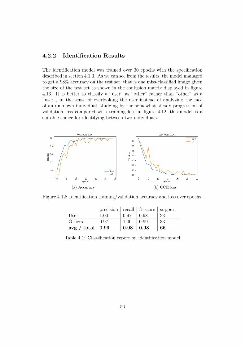
4.2.2 Identification Results
The identification model was trained over 30 epochs with the specificationdescribed in section 4.1.3. As we can see from the results, the model managedto get a 98% accuracy on the test set, that is one miss-classified image giventhe size of the test set as shown in the confusion matrix displayed in figure4.13. It is better to classify a ”user” as ”other” rather than ”other” as a”user”, in the sense of overlooking the user instead of analyzing the faceof an unknown individual. Judging by the somewhat steady progression ofvalidation loss compared with training loss in figure 4.12, this model is asuitable choice for identifying between two individuals.
(a) Accuracy (b) CCE loss
Figure 4.12: Identification training/validation accuracy and loss over epochs.
precision recall f1-score supportUser 1.00 0.97 0.98 33Others 0.97 1.00 0.99 33avg / total 0.99 0.98 0.98 66
Table 4.1: Classification report on identification model
56

Figure 4.13: Identification results confusion matrix.
4.2.3 Emotion Recognition Results
Information Regarding Training & Testing of Emotion Classifiers
Deep neural networks are stochastic processes and can produce a differentresult for separate training runs. A result of random initialization of weightsand other parameters during construction of a network. To get a statisticallyviable result, one should train each network over a series of runs, dependingon how much the result is fluctuating. In these experiments, 10 runs wereviewed as a suitable number for repetition of training and testing.
The two-class and four class models were trained for 30 epochs with arepetition of 10 runs. The seven-class model was trained for 60 epochs witha repetition of 10 runs. The tables below (4.2, 4.3 and 4.4) are from the topthree performances on the test set with a comparison between public (CK+)and personalized datasets. In the appendix section 8.2 a progression of lossand accuracy during training is presented for each of the three different casesof two, four and seven classes. The real-time evaluation was only done onthe models trained on the personalized dataset considering it showed the bestresults during offline training and testing, and it is the goal associated withthis thesis.
57

When progressing from two to four classes the model used for two classes,depicted in figure 4.7, was switched out with a model designed to handle abit more complex data structures which utilize batch normalization after thefirst layer as shown in figure 4.8.
Overall Results
In tables 4.2, 4.3, 4.4 the difference in accuracy’s between the CK+ andpersonalized dataset is increasing when adding more classes to predict. Infigure 4.15 an apparent difference is illustrated where the models’ perform-ances on two-, four-, and seven-classes is shown with average recognitionrate(accuracy). For seven classes the residual of percentage points equals13,3 on the average prediction accuracy, underlining the benefits of using apersonalized dataset for complicated facial expression recognition. The av-erage recognition rate of the top three results from the personalized modelis 98.6% on two classes, 96.3% on four classes and 97.6% on seven classes.It is somewhat surprising that the model performs better on seven classesthen four classes. It can be minor differences when initializing weights fortraining, which has given the seven class model a head start, or the caseof distinguishing degrees of one emotion which is the case in the four classdataset making it a bit harder to separate the classes. The most likely reasonis that the four-class model was trained for 30 epochs contrary to the sevenclass model which was trained for 60 epochs; thus it is not reasonable tocompare those two results. As for the CK+ model results, it managed to geta top three average of 94.3% on two classes, 91,3% on four classes and 84.3%on seven classes. When increasing from four to seven classes, the CK+ modelexperienced a notable dip in accuracy, even more than expected. Given thatthe CK+ dataset is quite skewed in the class distribution, the effect of thishas been prominent in the case of seven classes, allowing room for muchimprovement.
In figure 4.14, the activation map of layer 2 in the CNN model used forseven class emotion prediction on the personalized dataset is illustrated. Itis clear that the model is capable of focusing on correct regions in the facewhere most of the information describing that emotion lies, such as the eyesand the angle of the mouth.
58

(a) Input image (b) Activations
Figure 4.14: Activation map of layer 2 in personalized model.
Top 3 runs Accuracy1. 0.952. 0.943. 0.94Average 0.943Standard Deviation 0.005
(a) CK+
Top 3 runs Accuracy1. 1.002. 0.983. 0.98Average 0.986Standard Deviation 0.009
(b) Personalized
Table 4.2: Top 3 results from both datasets with two classes.
Top 3 runs Accuracy1. 0.942. 0.933. 0.87Average 0.913Standard Deviation 0.031
(a) CK+
Top 3 runs Accuracy1. 0.972. 0.963. 0.96Average 0.963Standard Deviation 0.005
(b) Personalized
Table 4.3: Top 3 results from both datasets with four classes.
59

Top 3 runs Accuracy1. 0.882. 0.833. 0.82Average 0.843Standard Deviation 0.026
(a) CK+
Top 3 runs Accuracy1. 0.982. 0.983. 0.97Average 0.976Standard Deviation 0.005
(b) Personalized
Table 4.4: Top 3 results from both datasets with seven classes.
Figure 4.15: Average model performances. (Two-classes left), (Four-classescenter), (Seven-classes right).
60

4.3 Real-Time Evaluation
(a) Predicted glad (b) Predicted happy (c) Predicted neutral
(d) Predicted sad (e) Predicted unknown
Figure 4.16: Predictions from the real-time evaluation of 4 classes.
This section presents the results from the real-time evaluation of a recor-ded 20 FPS video stream. The predictions were performed while recordingand the labels were assigned afterward to preserve the notion of live predic-tions.
By looking at the results in the confusion matrix presented in figures 4.17,4.18 and 4.19 real-time testing accuracy is somewhat lower than offline testingresults. The conditions when the personalized training set was constructedmay differ in many ways compared to conditions when testing in real-time.So it is to be expected that the real-time testing results show a less satisfyingoutcome than offline testing.
Given these priors, the personalized model can produce a total accuracy ofapproximately 93% correct classifications on two classes, 83% on four classesand 83% on seven classes. In figure 4.19 the emotion sad greatly overlapswith contempt and anger. A reason for this can be that my expression of sadcan easily be interpreted as one of the two other classes which then comesto light in real time testing. Contempt and disgust also seem to be easilymisclassified, given the action unit 12, Lip Corner Puller, is present in bothof these classes in the personalized dataset.
61

Real-Time Evaluation of Two Classes
Figure 4.17: Two-class confusion matrix of real-time evaluation.
Precision Recall F1-score SupportGlad 0.85 0.99 0.92 123Not-glad 0.99 0.89 0.94 183avg / total 0.9 0.93 0.93 306
Table 4.5: Classification report on two classes.
62

Real-Time Evaluation of Four Classes
Figure 4.18: Four-class confusion matrix of real-time evaluation.
Precision Recall F1-score SupportGlad 0.83 0.88 0.85 124Happy 0.96 0.87 0.91 52Neutral 0.90 0.75 0.82 84Sad 0.95 0.90 0.92 39avg/total 0.91 0.85 0.88 299
Table 4.6: Classification report on four classes
63

Real-Time Evaluation of Seven Classes
Figure 4.19: Seven-class confusion matrix of real-time evaluation.
precision recall f1-score supportAngry 1.00 0.85 0.92 208Contempt 0.94 0.67 0.79 203Disgust 0.66 1.00 0.80 61Fear 0.81 0.79 0.80 56Happy 0.86 0.93 0.89 124Sad 0.50 0.84 0.62 70Surprise 0.87 0.89 0.88 108avg / total 0.87 0.83 0.84 830
Table 4.7: Classification report on seven classes
64

Chapter 5
Emotion Recognition UsingSalient Features & RecurrentNeural Network in Video
In this chapter for research purposes, I will modify the work from Uddin,Khaksar and Torresen[1] by using a recurrent neural network instead of aconvolutional neural network as described in section 2.6 and feed the net-work with an image stream of 5-6 grayscale images contrary to depth images.Based on the robustness of Local Direction Pattern for facial expression de-scription presented in their paper, an adaptation of the feature extractionprocess is presented in this chapter. The idea is to classify the progressionof the facial expression using LDSP rather than looking at the expression ina single RGB-image. The proposed implementation is named LDSP-RNNin this thesis. This will not be implemented on the robot itself, but trainedand tested offline.
65
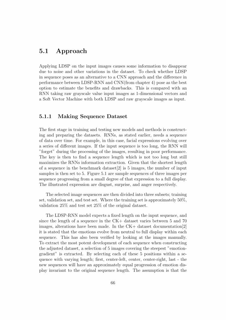
5.1 Approach
Applying LDSP on the input images causes some information to disappeardue to noise and other variations in the dataset. To check whether LDSPin sequence poses as an alternative to a CNN approach and the difference inperformance between LDSP-RNN and CNN(from chapter 4) pose as the bestoption to estimate the benefits and drawbacks. This is compared with anRNN taking raw grayscale value input images as 1-dimensional vectors anda Soft Vector Machine with both LDSP and raw grayscale images as input.
5.1.1 Making Sequence Dataset
The first stage in training and testing new models and methods is construct-ing and preparing the datasets. RNNs, as stated earlier, needs a sequenceof data over time. For example, in this case, facial expressions evolving overa series of different images. If the input sequence is too long, the RNN will”forget” during the processing of the images, resulting in poor performance.The key is then to find a sequence length which is not too long but stillmaximizes the RNNs information extraction. Given that the shortest lengthof a sequence in the benchmark dataset[2] is 5 images, the number of inputsamples is then set to 5. Figure 5.1 are sample sequences of three images persequence progressing from a small degree of that expression to a full display.The illustrated expression are disgust, surprise, and anger respectively.
The selected image sequences are then divided into three subsets; trainingset, validation set, and test set. Where the training set is approximately 50%,validation 25% and test set 25% of the original dataset.
The LDSP-RNN model expects a fixed length on the input sequence, andsince the length of a sequence in the CK+ dataset varies between 5 and 70images, alterations have been made. In the CK+ dataset documentation[2]it is stated that the emotions evolve from neutral to full display within eachsequence. This has also been verified by looking at the images manually.To extract the most potent development of each sequence when constructingthe adjusted dataset, a selection of 5 images covering the steepest ”emotion-gradient” is extracted. By selecting each of these 5 positions within a se-quence with varying length; first, center-left, center, center-right, last - thenew sequences will have an approximately equal progression of emotion dis-play invariant to the original sequence length. The assumption is that the
66

highest gradient lies in the middle of each sequence.
Figure 5.1: Emotions evolving over time.
Figure 5.2: Class distribution in sequence dataset.
5.1.2 Image Preprocessing
Before introducing the image sequences to the RNN model, feature extractionis needed to enhance the classification accuracy as described in the paper[1].The camera produces RGB images, but the benchmark dataset is grayscalecontrary to [1] which is trained on depth images. This may introduce morenoise compared to the previous work since the presence of edges is far greater
67
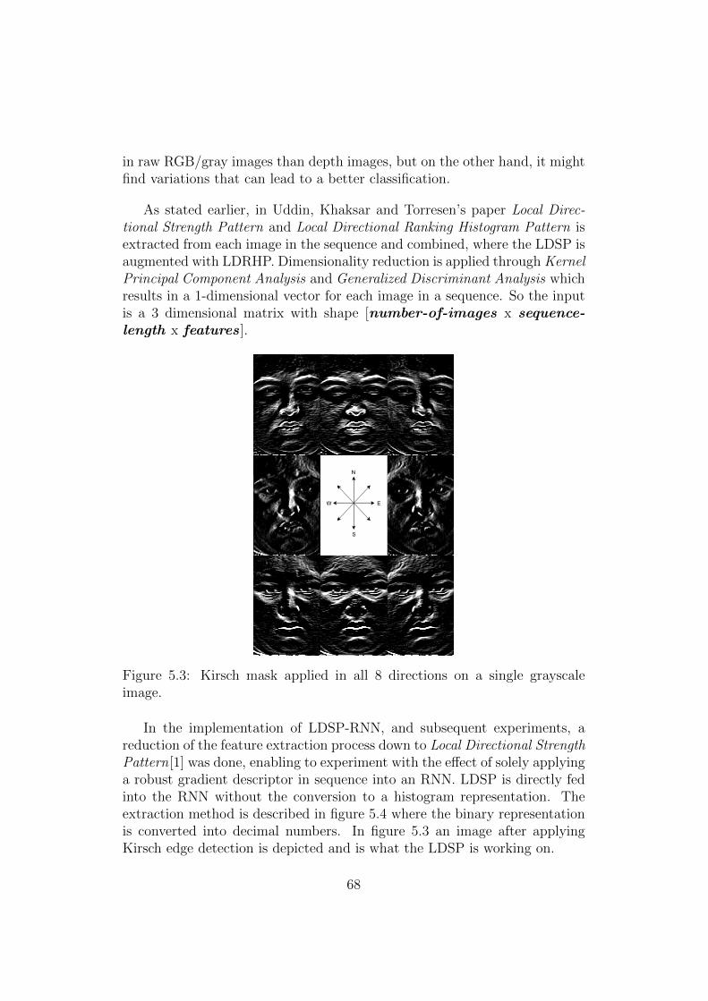
in raw RGB/gray images than depth images, but on the other hand, it mightfind variations that can lead to a better classification.
As stated earlier, in Uddin, Khaksar and Torresen’s paper Local Direc-tional Strength Pattern and Local Directional Ranking Histogram Pattern isextracted from each image in the sequence and combined, where the LDSP isaugmented with LDRHP. Dimensionality reduction is applied through KernelPrincipal Component Analysis and Generalized Discriminant Analysis whichresults in a 1-dimensional vector for each image in a sequence. So the inputis a 3 dimensional matrix with shape [number-of-images x sequence-length x features ].
Figure 5.3: Kirsch mask applied in all 8 directions on a single grayscaleimage.
In the implementation of LDSP-RNN, and subsequent experiments, areduction of the feature extraction process down to Local Directional StrengthPattern[1] was done, enabling to experiment with the effect of solely applyinga robust gradient descriptor in sequence into an RNN. LDSP is directly fedinto the RNN without the conversion to a histogram representation. Theextraction method is described in figure 5.4 where the binary representationis converted into decimal numbers. In figure 5.3 an image after applyingKirsch edge detection is depicted and is what the LDSP is working on.
68

Figure 5.4: Local Directional Strength Pattern on a 3x3 pixel neighborhoodin an image. The resulting LDSP code is now a representation for the centerpixel. This is repeated for all pixels of an image.
5.2 Experiments & Results
(a) Grayscale images (b) LDSP-features
Figure 5.5: 3D-plot of raw pixel values and LDSP-features on grayscale im-ages using LDA dimension reduction. Anger(blue) - Contempt(black) - Dis-gust(red) - Fear(cyan) - Happy(pink) - Sad(yellow) - Surprise(green)
69

(a) Grayscale im-age of sad
(b) Image afterKirsch mask andLDSP
Figure 5.6: Grayscale image before and after applying Kirsch mask and LocalDirectional Strength Pattern.
5.2.1 Visualization of Features
In figure 5.5 Linear Discriminant Analysis has been applied to the last frameof each sequence, reducing the dimension of the feature space down to 3 axes.It is done purely for illustration purposes, and is not applied on the data be-fore training of the LDSP-RNN. LDA chooses axes based on their ability toseparate the different classes. Compared to the 3D plot in Uddin, Khaksarand Torresen’s paper[1] where they manage to separate all the 6 differentfacial expressions with the use of Kernel Principal Component Analysis andGeneral Discriminant Analysis which utilizes a non-linear discriminant func-tion, the plot in figure 5.5 does not show as good separation. Since the imagesused in this experiment are raw grayscale images displaying seven differentemotions contrary to six class display on clear and highly detailed depthimages used in Uddin, Khaksar and Torresen’s paper, it is not expected toshow equally good results.
Defining a decision line between the grouped classes can be a challengingproblem to solve. The results in chapter 4 indicate a problem when tryingto separate seven different classes from the public dataset. The variations inthe CK+ dataset pose as the main obstacle when training a model, irrelevantto what type of deep learning architecture used. The results in this chapterbring light to the major faults associated with this dataset.
70

5.2.2 Training & Testing of Recurrent Neural NetworkApproach
By looking at the progression of the training in the LDSP-RNN approach,the model overfit very quickly indicating a possibility that the dataset is toosmall (see figure 5.7). With 325 samples in total (50% for training, 25%for testing and 25% for validation) where class representations vary greatly,none of the different approaches (listed in table 5.1) manage to achieve aclassification accuracy above 81%. The RNN model contains 100 recurrentcells, meaning the data is processed 100 times per time step, see figure 2.11.
Figure 5.7: Best training run of LDSP-RNN model.
RAW-IMAGE-RNN
When applying raw grayscale images as input to the RNN, consisting of 100recurrent cells and sigmoid activation, the performance comes short withroughly 11 percentage points on average recognition rate (72.8% contraryto 84.3%) compared to the seven class facial expression model in chapter 4which is trained on the peak expressions from the CK+ dataset (see section4.2).
LDSP-RNN
Introducing the RNN with LDSP feature vectors as input (LDSP-RNN),the average recognition rate is increased to 73.6%. The model has beentrained over 10 different runs, similar to the competing approaches in this
71

chapter. Though the RNN with raw images as input (RAW-IMAGE-RNN)produce a higher top recognition rate (81%), the average is less than LDSP-RNN’s average recognition rate, indicating that with the use of LDSP fea-tures it produces more robust results in the form of a lower standard deviationand a higher mean value (see table 5.1). Note that with so few testing imagesit is hard to conclude, but it indicates a possible outcome when fine-tuninghyperparameters and utilizes a better dataset for training.
Soft Vector Machine
As for comparing RNN to a standard image classifier, SVM is trained andtested on the same input data with a gamma parameter value of 0.01. Forboth cases of LDSP and raw grayscale images as input, it produced the samerecognition rate of 72%.
5.2.3 Overview of Results
In table 5.1 the result of 10 training iterations with 50 epochs per iterationis presented. Since deep neural networks are stochastic, a different resultcan be produced for each of the separate training runs, meaning multipleruns has to be applied to get statistically viable results. In figure 5.8 theaverage recognition rate from each approach on seven classes is illustratedand showing that LDSP-RNN produces the best outcome. The confusionmatrices from testing of LDSP-RNN and RAW-IMAGE-RNN are presentedin figure 5.9, highlighting the emotions that both approaches struggle toclassify. Contempt, anger, and sadness are the classes that show the mostprominent variations between the two models. Both anger and sadness arepresent in the cluster of inseparable classes illustrated in figure 5.5. Contemptis most likely misclassified due to low class representation in the training setas discussed in chapter 3.
72

Top Mean StdRNN w/ Raw image 0.81 0.728 0.086RNN w/ LDSP features 0.78 0.736 0.023SVM w/ Raw image 0.72 0.72 0SVM w/ LDSP features 0.72 0.72 0
Table 5.1: Test results from the different approaches with top, mean andstandard deviation of the 10 separate runs.
Figure 5.8: Model performances on raw image features and LDSP features.
73
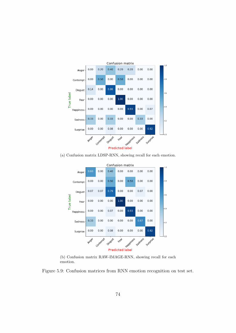
(a) Confusion matrix LDSP-RNN, showing recall for each emotion.
(b) Confusion matrix RAW-IMAGE-RNN, showing recall for eachemotion.
Figure 5.9: Confusion matrices from RNN emotion recognition on test set.
74

Chapter 6
Discussion
In this chapter results from both experiments, Real-time Face Detection,Identification & Emotion Recognition and Emotion Recognition Using SalientFeatures & RNN in video are discussed.
75

6.1 Real-Time Emotion Recognition Pipeline
The results have proved to be significant in the form of implementing afunctional real-time emotion recognition system and establishing the benefitsof using a personalized dataset contrary to a public dataset, although it iscommon knowledge that personalized models outperform generalized models.As discussed in chapter 3, there are some distinctions between the two datasetto be noted, such as different class distributions and RGB-images contrary tograyscale images. Despite these variations, the ten different runs testing themodels reveal that the model based on a personalized dataset outperformsthe model based on a public dataset in every instance, regardless of numberof classes to predict. On average, the the generalized model (CK+) achieveda recognition rate of 84.3% on seven classes, whereas the personalized modelgot a recognition rate of 97.6% on the same amount of classes.
Since the variance in the public dataset is more significant, a deeper clas-sification model is necessary to increase accuracy. A deeper neural networkis more capable of understanding a complex structure within the data, asdiscussed in the background and in LeCun, Bengio and Hinton’s paper[10].It is reasonable to assume that a deeper model would process data at a slowerrate since the number of calculations significantly increase with incrimina-tion of the number of hidden layers. The Multimodal Elderly Care Systemis primarily developed for assisting a single user, which means it has to fa-miliarize itself with that user. As shown in the results, a fairly shallow CNNcan accomplish an accuracy up to 98% on seven different expressions withthe use of techniques which is quite standard in today’s image classificationfield, such as Batch Normalization, Dropout, etc. The personalized modelcan learn more complex features that describes the user’s facial expressionwith fewer calculations, ergo faster processing.
When reviewing the results for each of the three cases (two-, four-, andseven-classes), one can see that the difference in accuracy between the CK+trained models and the personalized models with fewer classes at the outputare not as prominent as the models with a higher number of classes. Happyand Sad is quite different expressions, making the two-class problem an easiertask to solve. It is when the number of classes is increased that a notice-able difference in performance develops. For seven classes the personalizedmodels have almost ten percentage points higher accuracy than the CK+models. Also, the variance in both loss and accuracy of the CK+ models arequite high, as can be seen in the plots in the appendix. Figures 8.3 and 8.5
76

clearly indicate that the models are struggling to generalize good featuresfor classification. Since the variance in the CK+ dataset is much higher tobegin with, one should train the models with a lower learning rate or thenumber of validation samples should be increased to reduce the variance inthe validation accuracy and loss.
Validation accuracy and loss are only indications of how training pro-gresses. Since the training accuracy and loss looked promising and test ac-curacy somewhat matched what is to be expected, a decision not to increasethe number of validation samples was made since this would mean a reduc-tion in training samples. At the same time minimizing the differences inthe outset for both the personalized models and the generalized models, i.e.models trained on the CK+ public dataset.
One of the disadvantages of basing the models on a personalized dataset,is the accumulation process of a proper dataset containing every expressionof its user. Ideally, a well-performing model trained on a public datasetpose as the best option, since it does not need to be tailored to each personand therefore only needs to be trained once. However, as shown in thethesis, small, fast CNNs trained on multiple different faces cannot producethe desired result as it can with a personalized dataset.
6.2 Emotion Recognition Using Salient Fea-
tures & Recurrent Neural Network in Videos
In “Facial expression recognition using salient features and convolutionalneural network”[1] the model was trained on a depth image dataset and in-cluded a small experiment on a selected number of samples from the CK+dataset[2]. A different approach has been presented in this thesis basedon their work, by essentially reducing the feature extraction part to solelyKirsch edge detection[5] and Local Directional Strength Pattern[1]. A recur-rent neural network is trained with these features and called LDSP-RNN.It accomplished an average recognition rate of 73.6% on the test set. Theresults produced by this implementation cannot match what Uddin, Khak-sar and Torresen accomplished with their approach, due to several reasons.Firstly, it is not sustainable to compare the results, since they selected 40great samples with short sequence lengths and used a more comprehensivefeature extraction method. Nonetheless, it is not accurate to conclude that
77

the approach presented in this thesis come short of good results. Takinginto account that the RNN implementation considers all the seven differentclasses described in chapter 3 as well as utilizing all samples available inthe CK+ dataset, it leaves the possibility of an increased recognition rate ifpresented with better samples, i.e. filtering out samples that would distortthe network’s understanding of the problem.
The results obtained show a better average recognition rate using LDSP-RNN compared to RAW-IMAGE-RNN and LDSP-RNN outperformed a SoftVector Machine classification in both cases, as presented in table 5.1. Un-derstanding that edge detectors are sensitive to noise in the image is a keyfactor when selecting dataset to be used for training. Utilizing the wholeCK+ dataset for training has shown not to be ideal when applying an edgedetector for feature extraction. Noise can very easily be amplified, causingworse performance during training. Filtering techniques to remove noise poseas an option for further work within this implementation. Based on the res-ults presented in chapter 5 section 5.2, the LDSP-RNN approach has shownmuch potential, and with the correct parameters and training data it is mostlikely a suitable choice for classifying facial expressions in videos.
6.3 Ethical Dilemmas
Considering that the robot is aimed to be used in the users’ homes, there areseveral things to take into account regarding the implementation. The wel-fare and interests of the users must always be respected above anything else,and it is reasonable to discuss and evaluate the possibilities of malfunction,malpractice and exploitation of both the robot’s behavior and the inform-ation it can collect and process, combined with how this information is tobe distributed to persons of interest, i.e. family and healthcare personnel.The worst case scenario would be illegal distribution of private and sensitiveinformation about a reasonably vulnerable group in our population, seniors,due to their vulnerability when it comes to burglary and fraud. It is ourresponsibility as system designers to ensure that this does not occur.
With the rapid advancements in technology, it can be argued that safetyalso progresses. Such as our life expectancy with the help of modern medicineand technology, but that is not necessarily true in the case of informationsecurity. We now live in an era of information where we have reached aparadigm shift. Social media has contributed significantly to what we now
78
consider private information. Every internet site we visit collects informa-tion about its user and we trust online solutions with our pictures and otherprivate files. The only thing keeping this from being distributed across theworld for everyone to see is the security measures the storage providers haveimplemented. It is a constant battle between new security updates and ma-licious software trying to reach private data. The companies also have aresponsibility not to misuse the information provided by the user. Privacylegislation set by the government is there to ensure that privacy is respectedand not exploited in a negative way. However, there is always a risk that therules are not obeyed or that loopholes can be found and exploited.
Despite the risk we take entrusting that our information is safe, it hascome to good use. By allowing technology to make use of information thatis commonly not accessible, e.g. facial expressions, we can build and developsolutions which will help us and hopefully increase our standard of living.Introducing assisting technologies into elderly peoples’ homes may enable theuser to live at home for a more extended period, relieving resources to be usedelsewhere. By limiting the information the robot distributes to entrustedpersonnel, for example with encryption or a purer form of communication,it is possible to reduce the risk of sensitive information to go astray. Withthis in mind, the robot needs to process more of the information it collectslocally. Applying the implementation presented in chapter 4, a complexmental health analysis, compared to existing facial expression recognitionsystems, is possible without the need of cloud-based processing.
79

80

Chapter 7
Conclusion
This chapter presents a conclusion to the work presented in this thesis, in-cluding a proposition of future work related to chapter 4 and 5.
81

7.1 Real-Time Emotion Recognition Pipeline
The thesis has presented an approach for real-time emotion recognition ofhuman faces, which includes face detection and identification. By compar-ing public and private datasets, benefits of using a personalized dataset forclassification of multiple expressions and surpassing previous number of clas-sifications in related work have been established. The introduction describedlimitations which may be highlighted when using deep learning models, espe-cially image analysis, on a mobile robot without high performance hardware.With the presented approach, a personalized real-time emotion recognitionsystem with the ability of classifying seven different expressions is capableof running smoothly on a standard CPU, making it somewhat insensitive todifferent hardware specifications.
7.1.1 Is it Possible to Process Facial Expressions at aReasonable Speed in Real-Time on a StandardLaptop Computer, Without the Help of a GPU?
Yes, but with some precautions. When increasing the resolution of the inputimage stream, processing speed is dramatically reduced. This is not an issuewhen it comes to facial expression recognition since the CNN takes a fixedsize image as input, 100x100 pixels, but it is a problem for the face detectionalgorithm. The experiments are conducted on an image stream where eachframe has a resolution of 640x480 pixels. If the resolution is increased to1280x720 (HD-ready), the number of pixels to process triples in size. Withthe use of a GPU this resolution is not an issue, but with the assumptionthat all images have a resolution around 640x480, it is possible to detectfaces, identify and classify seven different facial expressions at 20 FPS.
7.1.2 How Well Does a Personalized Model PerformCompared to a Generalized Model?
A personalized model (trained on images from one person) will always out-perform a generalized model (trained on images of multiple people) in everyinstance of number of classes to predict (see section 4.2), but with the use ofa small customized CNNs complicated facial expressions can be recognized
82

with fewer training iterations and faster calculations.
7.2 Emotion Recognition Using Salient Fea-
tures & Recurrent Neural Network in Video
In this chapter(see chapter 5) an adaptation of the features extraction processpresented in [1] combined with a recurrent neural network was proposed, andnamed LDSP-RNN. With a standard RNN architecture with LDSP featuresas input, the model managed to get an average recognition rate of 73.6%on the test set of seven classes (see section 5.2). The CNN version’s topperforming model trained on the CK+ dataset got 88% accuracy (see section4.2), but with an average of around 84.3% over ten runs. Note that the LDSP-RNN was trained on the CK+ dataset and is therefore compared with theCNN model trained on the same dataset only with single image input. As astarting point, we can conclude that an LDSP-RNN model cannot competewith a CNN approach of single image peak emotion display classification.LDSP-RNN, on the other hand, produces an overall better recognition ratecompared to a RAW-IMAGE-RNN approach, proving that LDSP featurespose as a suitable option for classifying facial expressions and complies withthe findings presented in Uddin, Khaksar and Torresen’s paper[1].
7.2.1 Can Oriented Gradient Features in SequenceCombined With an RNN Pose as an Altern-ative to Standard CNNs?
Under the circumstances presented in this thesis it is not able to competewith the CNN approach, but with a better dataset combined with an expan-sion of the feature extraction process, the possibility of an equally or betterperformance is very much present.
7.3 Dissemination
During the work on this thesis, the Minister of Commerce (Torbjorn RoeIsaksen) and the Minister of Higher Education (Iselin Nybo) showed interest
83

in projects within Robotics and Artificial Intelligence due to higher prioritieswithin these fields of inventions. A presentation and live demonstration ofthe introduced approach for real-time emotion recognition was held, and wasbroadcasted on the evening news on NRK[52], and morning news on TV2[53].Links to both of the news stories are provided in the bibliography, see citationabove.
7.4 Future Work
7.4.1 Real-Time Emotion Recognition System
As discussed in section 6.1, a generalized model would be preferable whenconstructing a facial expression recognition system. This is due to the com-prehensive work of collecting a person dependent dataset for each user of thesystem. Utilizing more of the work described in “MobileFaceNets: EfficientCNNs for Accurate Real-time Face Verification on Mobile Devices” by Chenet al.[42], would enable the use of deeper CNNs with fewer parameters toupdate during training. It can be applied to all stages in the pipeline, giventhat a CNN currently is the preferred architecture for object detection andclassification. This can lead to experiments using the approach presentedin “HyperFace: A Deep Multi-task Learning Framework for Face Detection,Landmark Localization, Pose Estimation, and Gender Recognition” by Ran-jan, Patel and Chellappa[34], constraining face detection, identification andemotion recognition to a single convolutional neural network.
Due to time limitations on implementing and writing this thesis, testingof the proposed system on a moving robot in different environments has notbeen done, where areas of improvements are more easily detected.
7.4.2 Emotion Recognition Using Salient Features &Recurrent Neural Network in Video
During this thesis much attention has been put to the drawbacks of usingthe CK+ dataset[2], leaving the possibility of an improvement if a differentdataset had been used. Furthermore, experimenting with a greater varietyof RNN architectures and parameters can lead to new findings and hope-
84

fully increase the recognition rate of an LDSP-RNN on facial expressions.By expanding the feature extraction process before training an RNN, a bet-ter separation of expressions is possible. Based on the robustness of LDSPpresented in this thesis and [1], one can utilize the techniques used in Uddin,Khaksar and Torresen’s paper and expect better results. In section 5.2.1LDA was applied for vizualization of features in three dimensions. In on-going experiments LDA has been included in the feature extraction process,reducing the feature space down to 6 dimensions before applying RNN. It isshowing promising results, surpassing approaches presented in chapter 5.
85

Bibliography
[1] Md. Zia Uddin, Weria Khaksar and Jim Torresen. “Facial expressionrecognition using salient features and convolutional neural network”.In: IEEE Access 5 (2017), pp. 26146–26161. issn: 21693536. doi: 10.1109/ACCESS.2017.2777003. url: http://ieeexplore.ieee.org/document/8119492/.
[2] P. Lucey et al. “The extended cohn-kande dataset (CK+): A com-plete facial expression dataset for action unit and emotionspecified ex-pression”. In: Cvprw July (2010), pp. 94–101. issn: 01628828. doi:10.1109/ISIEA.2010.5679500.
[3] Timo Ahonen, Abdenour Hadid and Matti Pietikainen. “Face descrip-tion with local binary patterns: Application to face recognition”. In:IEEE Transactions on Pattern Analysis and Machine Intelligence 28.12(2006), pp. 2037–2041. issn: 01628828. doi: 10.1109/TPAMI.2006.244.
[4] Taskeed Jabid, Md Hasanul Kabir and Oksam Chae. “Local directionalpattern (LDP) for face recognition”. In: International Journal of In-novative Computing, Information and Control 8.4 (2012), pp. 2423–2437. issn: 13494198. doi: 10.1109/ICIP.2010.5652374.
[5] Taskeed Jabid, Md. Hasanul Kabir and Oksam Chae. “Local Direc-tional Pattern (LDP) – A Robust Image Descriptor for ObjectRecognition”. In: 2010 7th IEEE International Conference on AdvancedVideo and Signal Based Surveillance. IEEE, Aug. 2010, pp. 482–487.isbn: 978-1-4244-8310-5. doi: 10.1109/AVSS.2010.17. url: http://ieeexplore.ieee.org/document/5597095/.
[6] Kamrul Hasan Talukder and Koichi Harada. Haar Wavelet Based Ap-proach for Image Compression and Quality Assessment of CompressedImage. Tech. rep. url: https://arxiv.org/pdf/1010.4084.pdf.
86

[7] Constantine P Papageorgiou, Michael Oren and Tomaso Poggio. AGeneral Framework for Object Detection. Tech. rep. url: https://pdfs.semanticscholar.org/76f5/60991d56ad689ec32f9e9d13291e0193f4cf.
pdf.
[8] Paul Viola and Mj Jones. “Robust real-time face detection”. In: In-ternational journal of computer vision 57.2 (2004), pp. 137–154. issn:0920-5691. doi: 10.1023/B:VISI.0000013087.49260.fb. url: http://link.springer.com/article/10.1023/B:VISI.0000013087.
49260.fb.
[9] Navneet Dalal and Bill Triggs. “Histograms of oriented gradients for hu-man detection”. In: Proceedings - 2005 IEEE Computer Society Confer-ence on Computer Vision and Pattern Recognition, CVPR 2005. Vol. I.IEEE, 2005, pp. 886–893. isbn: 0769523722. doi: 10.1109/CVPR.2005.177. url: http://ieeexplore.ieee.org/document/1467360/.
[10] Yann LeCun, Yoshua Bengio and Geoffrey Hinton. “Deep learning”.In: Nature 521.7553 (May 2015), pp. 436–444. issn: 0028-0836. doi:10.1038/nature14539. url: http://www.nature.com/articles/nature14539.
[11] Shima Alizadeh and Azar Fazel. “Convolutional Neural Networks forFacial Expression Recognition”. In: arXiv preprint arXiv:1704.06756(2017). issn: 21945357. doi: 10.1007/978-3-319-47952-1\_6.url: http://arxiv.org/abs/1704.06756.
[12] Ihor Paliy. “Face Detection Using Haar -like Features Cascade andConvolutional Neural Network”. In: 2008 Proceedings of InternationalConference on Modern Problems of Radio Engineering, Telecommu-nications and Computer Science (2008), pp. 375–377. url: http://ieeexplore.ieee.org/xpl/articleDetails.jsp?arnumber=5423372.
[13] Steve Lawrence et al. “Face Recognition : A Convolutional Neural Net-work Approach”. In: Neural Networks 8.1 (1997), pp. 98–113. url:http : / / ieeexplore . ieee . org / lpdocs / epic03 / wrapper . htm ?
arnumber=554195.
[14] S Guo, S Chen and Y Li. “Face recognition based on convolutionalneural network & support vector machine”. In: 2016 IEEE Interna-tional Conference on Information and Automation, IEEE ICIA 2016August (2017), pp. 1787–1792. doi: 10.1109/ICInfA.2016.7832107.url: https://www.scopus.com/inward/record.uri?eid=2-s2.0-85015775572&doi=10.1109%2FICInfA.2016.7832107&partnerID=
40&md5=2523c4287769e853e4620a26fa58f701.
87
[15] Yann LeCun et al. “A theoretical framework for back-propagation”. In:Proceedings of the 1988 connectionist models summer school. Vol. 1.CMU, Pittsburgh, Pa: Morgan Kaufmann. 1988, pp. 21–28.
[16] George E. Dahl, Tara N. Sainath and Geoffrey E. Hinton. “Improvingdeep neural networks for LVCSR using rectified linear units and dro-pout”. In: 2013 IEEE International Conference on Acoustics, Speechand Signal Processing. IEEE, May 2013, pp. 8609–8613. isbn: 978-1-4799-0356-6. doi: 10.1109/ICASSP.2013.6639346. url: http:
//ieeexplore.ieee.org/document/6639346/.
[17] Zhou Wang and A.C. Bovik. “Mean squared error: Love it or leave it?A new look at Signal Fidelity Measures”. In: IEEE Signal ProcessingMagazine 26.1 (Jan. 2009), pp. 98–117. issn: 1053-5888. doi: 10.1109/MSP.2008.930649. url: http://ieeexplore.ieee.org/document/4775883/.
[18] Sergey Ioffe and Christian Szegedy. “Batch Normalization: Accelerat-ing Deep Network Training by Reducing Internal Covariate Shift”. In:(Feb. 2015). url: http://arxiv.org/abs/1502.03167.
[19] Jimmy Lei Ba, Jamie Ryan Kiros and Geoffrey E. Hinton. “Layer Nor-malization”. In: (July 2016). url: http://arxiv.org/abs/1607.06450.
[20] Yanghao Li et al. “Revisiting Batch Normalization For Practical Do-main Adaptation”. In: (Mar. 2016). url: http://arxiv.org/abs/1603.04779.
[21] Nitish Srivastava et al. “Dropout: A Simple Way to Prevent NeuralNetworks from Overfitting”. In: Journal of Machine Learning Research15 (2014), pp. 1929–1958. issn: 15337928. doi: 10.1214/12-AOS1000.url: http://jmlr.org/papers/volume15/srivastava14a.old/
srivastava14a.pdf.
[22] Pavel Golik, Patrick Doetsch and Hermann Ney. Cross-Entropy vs.Squared Error Training: a Theoretical and Experimental Comparison.Tech. rep. 2013. url: https://www.isca- speech.org/archive/
archive_papers/interspeech_2013/i13_1756.pdf.
[23] Douglas M. Kline and Victor L. Berardi. “Revisiting squared-errorand cross-entropy functions for training neural network classifiers”.In: Neural Computing and Applications 14.4 (Dec. 2005), pp. 310–318.issn: 0941-0643. doi: 10.1007/s00521- 005- 0467- y. url: http:
//link.springer.com/10.1007/s00521-005-0467-y.
88

[24] Zhilu Zhang and Mert R. Sabuncu. “Generalized Cross Entropy Lossfor Training Deep Neural Networks with Noisy Labels”. In: (May 2018).url: http://arxiv.org/abs/1805.07836.
[25] Diederik P Kingma and Jimmy Lei Ba. ADAM: A METHOD FORSTOCHASTIC OPTIMIZATION. Tech. rep. url: https://arxiv.org/pdf/1412.6980.pdf.
[26] Tijmen Tieleman and Geoffrey Hinton. “Lecture 6.5-rmsprop: Dividethe gradient by a running average of its recent magnitude”. In: COURS-ERA: Neural networks for machine learning 4.2 (2012), pp. 26–31.
[27] John Duchi, Elad Hazan and Yoram Singer. “Adaptive SubgradientMethods for Online Learning and Stochastic Optimization”. In: Journalof Machine Learning Research 12.Jul (2011), pp. 2121–2159. issn: ISSN1533-7928. url: http://www.jmlr.org/papers/v12/duchi11a.html.
[28] Luis Perez and Jason Wang. “The Effectiveness of Data Augmentationin Image Classification using Deep Learning”. In: (Dec. 2017). url:https://arxiv.org/abs/1712.04621.
[29] Ian Goodfellow et al. “Generative Adversarial Nets”. In: Advances inNeural Information Processing Systems 27. Ed. by Z Ghahramani et al.Curran Associates, Inc., 2014, pp. 2672–2680. url: http://papers.nips.cc/paper/5423-generative-adversarial-nets.pdf.
[30] Zack Thoutt. GOT Book 6 Generator. url: https://github.com/zackthoutt/got-book-6.
[31] Samira Ebrahimi Kahou et al. “Recurrent Neural Networks for EmotionRecognition in Video”. In: Proceedings of the 2015 ACM on Interna-tional Conference on Multimodal Interaction - ICMI ’15. New York,New York, USA: ACM Press, 2015, pp. 467–474. isbn: 9781450339124.doi: 10.1145/2818346.2830596. url: http://dl.acm.org/citation.cfm?doid=2818346.2830596.
[32] Quoc V. Le, Navdeep Jaitly and Geoffrey E. Hinton. “A Simple Wayto Initialize Recurrent Networks of Rectified Linear Units”. In: (Apr.2015). url: https://arxiv.org/abs/1504.00941.
[33] Ali Sharifara, Mohd Shafry Mohd Rahim and Yasaman Anisi. “A gen-eral review of human face detection including a study of neural net-works and Haar feature-based cascade classifier in face detection”. In:Proceedings - 2014 International Symposium on Biometrics and Se-curity Technologies, ISBAST 2014 (2015), pp. 73–78. doi: 10.1109/ISBAST.2014.7013097.
89

[34] Rajeev Ranjan, Vishal M. Patel and Rama Chellappa. “HyperFace: ADeep Multi-task Learning Framework for Face Detection, LandmarkLocalization, Pose Estimation, and Gender Recognition”. In: IEEETransactions on Pattern Analysis and Machine Intelligence XX.Xx(2017), pp. 1–16. issn: 01628828. doi: 10.1109/TPAMI.2017.2781233.
[35] Haoxiang Li et al. “A convolutional neural network cascade for facedetection”. In: Cvpr (2015), pp. 5325–5334. issn: 1063-6919. doi: 10.1109/CVPR.2015.7299170.
[36] Davis. E. King. “Dlib-ml: A Machine Learning Toolkit”. In: Journal ofMachine Learning Research 10 (2009), pp. 1755–1758. issn: 15324435.doi: 10.1145/1577069.1755843. url: http://jmlr.csail.mit.edu/papers/v10/king09a.html.
[37] G Bradski. “The OpenCV Library”. In: Dr Dobbs Journal of SoftwareTools 25 (2000), pp. 120–125. issn: 1044-789X. doi: 10.1111/0023-8333.50.s1.10. url: http://opencv.willowgarage.com.
[38] Joao F. Henriques et al. “Exploiting the Circulant Structure of Tracking-by-Detection with Kernels”. In: Springer, Berlin, Heidelberg, 2012,pp. 702–715. doi: 10.1007/978-3-642-33765-9\_50. url: http://link.springer.com/10.1007/978-3-642-33765-9_50.
[39] Martin Danelljan et al. “Adaptive Color Attributes for Real-Time VisualTracking”. In: The IEEE Conference on Computer Vision and PatternRecognition (CVPR). 2014.
[40] haar-feature-image. url: http://siret.ms.mff.cuni.cz/facereco/method.
[41] Yaniv Taigman et al. “DeepFace: Closing the gap to human-level per-formance in face verification”. In: Proceedings of the IEEE ComputerSociety Conference on Computer Vision and Pattern Recognition (2014),pp. 1701–1708. issn: 10636919. doi: 10.1109/CVPR.2014.220.
[42] Sheng Chen et al. “MobileFaceNets: Efficient CNNs for Accurate Real-time Face Verification on Mobile Devices”. In: (Apr. 2018). issn: 16113349.doi: arXiv:1804.07573v2. url: http://arxiv.org/abs/1804.
07573.
[43] Karen Simonyan and Andrew Zisserman. “Very Deep ConvolutionalNetworks for Large-Scale Image Recognition”. In: International Con-ference on Learning Representations (ICRL) (Sept. 2015), pp. 1–14.issn: 09505849. doi: 10.1016/j.infsof.2008.09.005. url: http://arxiv.org/abs/1409.1556.
90

[44] Md. Uddin, J. Lee and T.-S. Kim. “An enhanced independent component-based human facial expression recognition from video”. In: IEEE Trans-actions on Consumer Electronics 55.4 (2009), pp. 2216–2224. issn:0098-3063. doi: 10.1109/TCE.2009.5373791.
[45] Md Hasanul Kabir et al. “Facial Expression Recognition from DepthVideo with Patterns of Oriented Motion Flow”. In: IEEE Access 5(2017), pp. 8880–8889. issn: 21693536. doi: 10.1109/ACCESS.2017.2704087.
[46] N. Sebe et al. “Authentic facial expression analysis”. In: Image andVision Computing 25.12 (2007), pp. 1856–1863. issn: 02628856. doi:10.1016/j.imavis.2005.12.021.
[47] Ian Goodfellow et al. Challenges in Representation Learning: A reporton three machine learning contests. 2013. url: http://arxiv.org/abs/1307.0414.
[48] Paul Ekman and Wallace V Friesen. Manual for the facial action codingsystem. Consulting Psychologists Press, 1978.
[49] M Jordan, J Kleinberg and B Scholkopf. Pattern Recognition and Ma-chine Learning. Tech. rep. url: http://users.isr.ist.utl.pt/
~wurmd/Livros/school/Bishop%20-%20Pattern%20Recognition%
20And%20Machine%20Learning%20-%20Springer%20%202006.pdf.
[50] Scale Image. url: https://sites.google.com/site/5kk73gpu2012/assignment/viola-jones-face-detection#TOC-Image-Pyramid.
[51] object detection - OpenCV detectMultiScale() minNeighbors parameter- Stack Overflow. url: https://stackoverflow.com/questions/22249579/opencv-detectmultiscale-minneighbors-parameter.
[52] NRK Evening News. 2018. url: https://tv.nrk.no/serie/kveldsnytt/NNFA23090218/02-09-2018.
[53] TV2 Morning News. 2018. url: https://youtu.be/m5yu2BimALk.
91

92

Chapter 8
Appendix
8.1 Sensors, Software & Hardware
• Samsung ultrabook series 9
• Intel Core i7-3517U CPU - 1.90GHz x 4
• Microsoft 1080p HD sensor camera
• Ubuntu 16.04
• Python 3.6.6
• TensorFlow 1.8
• Keras 2.1.6
• OpenCV 3.4.2.17
• dlib 19.7.0
93

8.2 Emotion Recognition Training Plots
8.2.1 Two Classes
(a) Accuracy run 7/10 (b) Loss run 7/10
(c) Accuracy run 8/10 (d) Loss run 8/10
(e) Accuracy run 10/10 (f) Accuracy run 10/10
Figure 8.1: Cohn-Kanade - Two-class training and validation accuracy andcategorical cross entropy loss over number of epochs
94

(a) Accuracy run 5/10 (b) Loss run 5/10
(c) Accuracy run 8/10 (d) Loss run 8/10
(e) Accuracy run 10/10 (f) Loss run 10/10
Figure 8.2: Personalized - Two-class training and validation accuracy andcategorical cross entropy loss over number of epochs
95

8.2.2 Four Classes
(a) Accuracy run 1/10 (b) Loss run 1/10
(c) Accuracy run 4/10 (d) Loss run 4/10
(e) Accuracy run 9/10 (f) Loss run 9/10
Figure 8.3: Cohn-Kanade - Four-class training and validation accuracy andcategorical cross entropy loss over number of epochs
96

(a) Accuracy run 2/10 (b) Loss run 2/10
(c) Accuracy run 5/10 (d) Loss run 5/10
(e) Accuracy run 10/10 (f) Loss run 10/10
Figure 8.4: Personalized - Four-class training and validation accuracy andcategorical cross entropy loss over number of epochs.
97

8.2.3 Seven Classes
(a) Accuracy run 1/10 (b) Loss run 1/10
(c) Accuracy run 2/10 (d) Loss run 2/10
(e) Accuracy 8/10 (f) Loss 8/10
Figure 8.5: Cohn-Kanade - Seven-class training and validation accuracy andcategorical cross entropy loss over number of epochs.
98

(a) Accuracy run 1/10 (b) Loss run 1/10
(c) Accuracy run 3/10 (d) Loss run 3/10
(e) Accuracy 5/10 (f) Loss 5/10
Figure 8.6: Personalized - Seven-class training and validation accuracy andcategorical cross entropy loss over number of epochs.
99


![Basic and depression specific emotion identification in ...webdocs.cs.ualberta.ca/~zaiane/postscript/CICLING19-1.pdf · label emotion mining from text [2,11,17]. With the increasing](https://img.dokumen.tips/doc/110x75/5f4a6fb08857b1069945e82f/basic-and-depression-speciic-emotion-identiication-in-zaianepostscriptcicling19-1pdf.jpg)