LARGE EDDY SIMULATION OF REAL

WALL BOUNDED FLOWS

Christer FurebyThe Swedish Defence Research Agency – FOIWeapons & ProtectionGrindsjön Research CenterStockholm, Sweden

Chalmers University of TechnologyDept of Naval ArchitectureGothenburg, Sweden

AcknowledgementFOI, Stockholm, SwedenN. Alin, M. Berglund, E. Lillberg, M. Liefendahl, O. Parmhed,U. Svennberg, N. Wikström, J. Tegnér

CTH, Gothenburg, SwedenR. Bensow, T. Persson, N. Svanstedt

NRL, Washington DC, USAF.F. Grinstein et al

LANL, Los Alamos, NM, USAW. Rider

GaTech, Atlanta GA, USAS. Menon

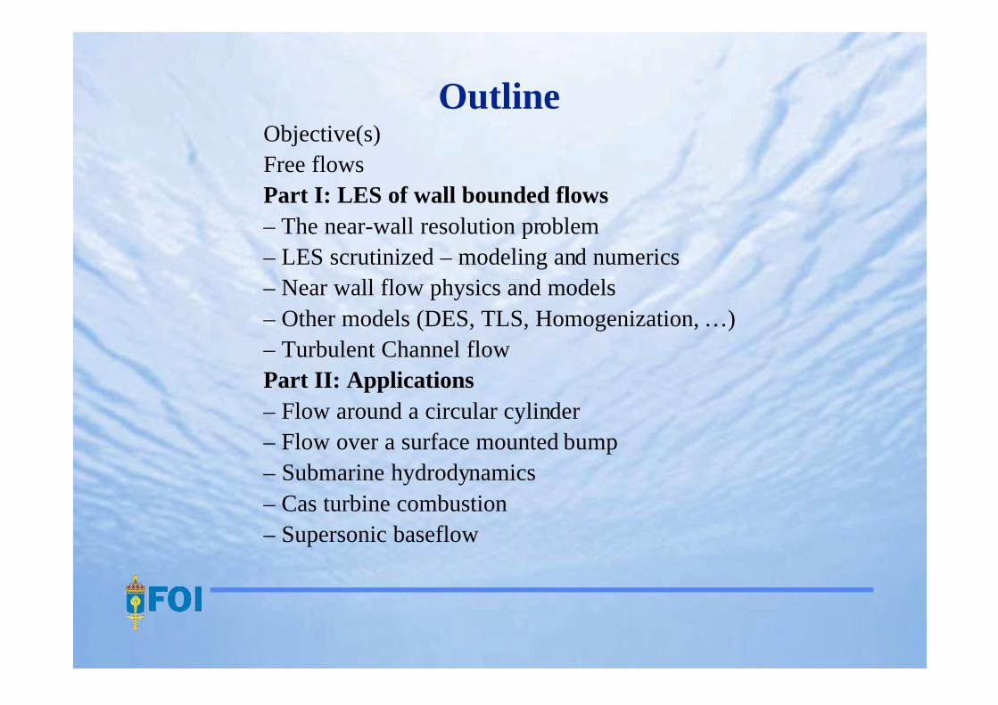
OutlineObjective(s)Free flowsPart I: LES of wall bounded flows– The near-wall resolution problem– LES scrutinized – modeling and numerics– Near wall flow physics and models– Other models (DES, TLS, Homogenization, …)– Turbulent Channel flowPart II: Applications– Flow around a circular cylinder– Flow over a surface mounted bump– Submarine hydrodynamics– Cas turbine combustion– Supersonic baseflow

Objective

‘bridging the gap’

The Navier-Stokes Equations

Conservation of massEulers 1st lawEulers 2nd lawThe energy lawThe entropy inequality

Constitutive equationsdescribing the propertiesof the fluidsT, h, p, ε, …

Field equationsReynolds transporttheorem

Modern Continuum Mechanics (Truesdell, Noll, Gurtin, …)

∂ ρ ρ

∂ ρ ρ ρ

∂ ρ ρ ρσ

ε ρ

λ µ λ µ µ

κ

t

t

t

V

Dp

e e

c T T p RT

tr tr

T

( ) ( )

( ) ( )

( ) ( )

( ),

( ) (( ) )

+∇⋅ =

+∇⋅ =−∇ +∇⋅ +

+∇⋅ =∇⋅ + ⋅ +

= − =

= + = + +

= ∇

⊗

v

v v v S f

v h S D

S D I D D I D

h

0

2 20

23

∂ ν

ννt p

p

( ) ( ) ( )

( )

v v v v f

v v v v fS D

+∇⋅ =−∇ +∇⋅ ∇ +

∇⋅ = ⇒ =∇ ∇ − +∇⋅=

⊗

⊗022 ∆

Turbulence in Free FlowsSmallest scales characterized by strong, slender tube-like filament vortices scaling with lk.

Turbulent flows of practical importance are in-herently 3D, unsteady and subjected to strong mean inhomogeneities and rapid deformations.

Porter & Woodward10

010

110

210

-5

10-4

10-3

10-2

10-1

100

101

E

k

largescales

energycontainingintegralscales

inertialsubrange

viscoussubrange

k–5/3

1/lΙ 1/lΤ 1/lΚ

dissipation

production

The (Free Flow) Resolution ProblemIn Direct Numerical Simulation (DNS) all scales needs to be resolvedi.e.⇒

taking also the time into account

For typical engineering applications:Re≈108 ⇒ cost∝1024

Discretization costs 103 operations per grid points⇒ cost∝1027

Earth simulator: 41 Tflops/s1027 / 41·1012 ≈ 770 år !

On the expensive side!

Mohrs law

Modeling / cost reduction required!

l lI K I/ Re /= 3 4

cos / Re /t I K I∝( ) =l l3 9 4

cos Ret I∝ 3

DES J. Forsythe

100

101

102

10-5

10-4

10-3

10-2

10-1

100

101

E

k

largescales

energycontainingintegralscales

inertialsubrange

viscoussubrange

k–5/3

1/lΙ 1/lΤ 1/lΚ

Computed in DNS

Computedin RANS Modeled in RANS

Computed in LESModeledin LES

?

DNS, LES, DES and RANSDirect Numerical Simulation (DNS)Solve the NSE without modelingN∝Re9/4, high numerical accuracyAll physics correctly treated

Large Eddy Simulation (LES)Solve the NSE with partial modelingN∝Re3/2 , high numerical accuracy

Subgrid turbulence modelsPhysics on macro & meso scales correctly treated

Detached Eddy Simulation (DES)Solve the NSE with partial modelingLES in the free-flow regionRANS in boundary layer

Reynolds Average Navier Stokes (RANS)2D/3D solution with turbulence modelingThe model often dictates the resolutionDoes not necessarily converge to DNS

Classical validation problem for LES (RANS)ReD=95,000EXP: Crow & Champagne, 1971 Capp, Hussein & George, 1994Grid: ~ 900,000

Free Flows: The Turbulent Round Jet

Axial velocity

Vorticity: Q=(||D||2-||W||2)

CHG experiment ideal for LES validation:• Thin nozzle lips• Top-hat shaped velocity profile• No inlet fluctuations

mixing regionx/D<10

transition region10<x/D<30

self-similar regionx/D>30

0 10 20 30 40 500

0.2

0.4

0.6

0.8

1

1.2

(<v>

-ve)/

(v0-v

e)

x/D

LES MIXEDMILESLES OEEVMEXP Crow & ChampagneEXP Cohen & WygnanskiEXP LauEXP Anselmet & Fulashier

0 10 20 30 40 500

0.02

0.04

0.06

0.08

0.1

0.12

0.14

0.16

0.18

0.2

(vpr

ime)

/(v 0-v

e)

x/D

LES MIXEDMILESLES OEEVMEXP Crow & ChampagneEXP Lau

Rms velocity fluctuation @ CLMean velocity @ CL

-4 -2 0 2 4 6 8

0

0.2

0.4

0.6

0.8

1

1.2(<

v>-v

e)/(v

0-ve)

r/D

LES MIXED x/D=4LES MIXED x/D=8LES MIXED x/D=16LES MIXED x/D=32MILES x/D=4MILES x/D=8MILES x/D=16MILES x/D=32LES OEEVM x/D=4LES OEEVM x/D=8LES OEEVM x/D=16LES OEEVM x/D=32EXP x/D=4EXP x/D=8EXP x/D=16

Mean velocity @ x/D=4, 8, 16

Free Flows: The Turbulent Round Jet

The Near-Wall Resolution ProblemCentral issues of wall bounded flows are the forms of the mean velocity profilesand the friction laws, describing the shear stress exerted by the fluid on the wall.

Outer region• Dissipation• Stucture size ~ δ99

Inner region• Production of TKE• Dissipation• Structures: streaks, …

Streaks at y+≈≈≈≈15L+≈1000r+≈10∆h+≈10∆z+≈100

Near-wall scaling (+ units)l=ν/uτu=|ττττw|1/2

ττττw=ν((∇v)t)w

||D||2–||W||2<0vx

~2400·l

~1000·llow speedstreak

high speed streak

LES @ Reττττ=395

To resolve all dynamically important near-wall structures requires a grid of

∆x≈100, ∆y≈2 and ∆z≈10

Too expensive!Models required!

Less universal properties than free flows

Flow dominated by:– BL dynamics– streaks– Ω-shaped vortices– p fluctuations– ejections

Streaks as frequent ashairpin vortices in free flows

Almost universal velocity profile

The Near-Wall Resolution Problem cont’d

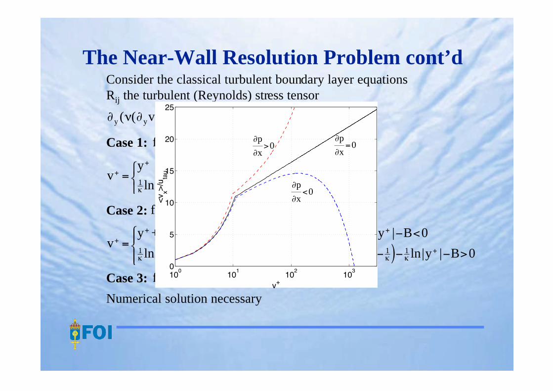
The Near-Wall Resolution Problem cont’dConsider the classical turbulent boundary layer equationsRij the turbulent (Reynolds) stress tensor

Case 1:

Case 2:

Case 3:

Numerical solution necessary

fi = + +∂ ∂ ∂i t i j i jp v v v( )

∂ ν ∂ ∂ ∂ ∂y y i iy i i t i j i jv R f p v v v( ( ) ) ; ( ) ( ) ( )− = = + + fi

f i = ⇒ −0 2ν ∂( )y i iv R

vy y y

y B y yy+

+ + +

+ + ++=

≤

+ >

≈ if

if 0

10

0 11 3,

ln| | ,.

κ

f i = ⇒ − =∂ ∂ ν ∂ ∂i y y i iy ip v R p( ( ) ) ( )

vy p y p y B

y p B y p y B

yu i

yu i

y

yu i

yu i

y+

+ + +

+ + +=

+ −( )− − <

+ + + −( )− − >

+ + +

+ + +

+ if

if

ν νκ κ

κνκ

νκ κ

τ τ

τ τ

∂ ∂

∂ ∂

( ) ( ) ( ) ln| |

ln| | ( ) ( ) ln| |

2

3 3

3

2 21 1

12

1 1

0

0

10

010

110

210

30

5

10

15

20

25

<v x>

/uta

u

y+

∂

∂

p

x>0

∂

∂

p

x=0

∂

∂

p

x<0

∇⋅ =

+∇⋅ =−∇ +∇⋅ − + + ⊗

( )

( ) ( ) ( )

v

v v v S B f m

m

pt∂

B v v v v v m v v I S= − = ∗∇ = ∗∇ + −⊗ ⊗ ⊗( ), [ , ] , [ , ]( ) m G G p

Filtering the NSE

LES – FilteringConsider the incompressible NSE

The NSE are low-pass-filtered in order to remove the small-scale eddies

v v x x v x x= ∗ = − ′ ′∫ ′G G t dD ( ; ) ( , ) ,∆ 3 etc.

Filtering of a gradient, i.e. ∇Φ

yields a commutation error

Filtering and differentiation cannot be unconditionally exchanged!

∇ = ∇∫ ′ +∫ ′ + =∇ + ∗ ∇ +∈ ∈Φ Φ Φ Φ Φ Φ ∆ Φ∆ ∆G G d d G GD D x D x DG G( ) ( ) ( ) ( )x x n n3 3∂∂

∂∂∂ ∂

[ , ] ( ) ( )G GGx D∗∇ =∇ −∇ = ∗ ∇ + ∈Φ Φ Φ Φ ∆ Φ∆

∂∂ ∂n

Subgrid stress tensor- to be modeled

Commutation terms

LES – Numerical MethodsThe finite volume method is based on the integral form of the governing PDEsover each control volume. → Flow properties conserved

Gauss theorem + localization theorem

Finite Volume discretization

• Crank-Nicholson time-integration

• Linear reconstruction of convective fluxes

• Central difference approx. for inner derivatives in and

⇒ 2nd order central scheme

PISO pressure-velocity decoupling algorithm

Segregated approach (α-stable with Co<0.5)

βδ

ρ

βδα β

i

P

i

P

tV f

C n if

i Pn i t

V fC v

fD v

fB v n i

f i Pn i

im

F

p t

∆ +

+ ∆ + +=

∑ =

+ + +∑ =− ∇ ∆∑

[ ]

( ( ) [ ] ) ( )

,

, , ,

0

0 v F F FP •

• N

dA

f

d

!

!

!

!

!

FfC v,

FfD v, Ff

B v,

LES – ModelingModel the subgrid stress tensor, which classically can be decomposed as

L: Leonard terms interactions inbetween resolved eddies – no model required!

C: cross terms interactions between resolved and subgrid eddies

R: Reynods terms interactions inbetween subgrid eddies

B v v v v v v v v v v L C R= −( )+ ′+ ′( )+ ′ ′( )= + +⊗ ⊗ ⊗ ⊗ ⊗

Need to assure that the models employed have the same mathematicalproperties as the terms they emulate:

Frame Indifference

as applied to the filtered NSE yieldsx X c Q x X X*( , ) ( ) ( )( ( , ) ), *t t t t t t= + − = + τ

B QBQ

L QLQ C QCQ R QRQ

*

* , * , *

=

= + = − =

T

T T TΛΛ ΛΛ

SS*

LES – Modeling cont’dFunctional Modeling

Reproduce the effects of the small-scale eddies on the resolved onesPhysical considerations + nature of interactions

Eddy Viscosity Models (EVM)

Smagorinsky EVM (Smagorinsky, 1963)

One Equation EVM (Schumann, 1975, Menon & Fureby, 1995 …)

Model coefficients evaluated from the k–5/3 shape or dynamically

Generally robustPoor correlation with DNS dataEignvectors not parallel with those of true BIncorrect near-wall scaling → Damping functions (van-Driest, …)

B B B I D BD ktr k tr= − =− =13

122( ) ,ν

ν ∂ ν ν εk k t kc k k k k c k= +∇⋅ =− ⋅ +∇⋅ + ∇ +∆ ∆1 2 3 2/ /, ( ) ( ) (( ) ) / v B D

νk D Ic k c= =∆ ∆2 2 2|| ||, || ||D D

LES – Modeling cont’dStructural Modeling

∂ ν ε εtT T

k D Ddiv c k( ) ( ) ( ) ( )B B v LB BL B B D I+ =− + +∇⋅ ∇ − + −⊗ 125

23

Aim at predicting the subgrid stress tensor and the subgrid force

Differential Subgrid Stress Models (Deardorff, 1973, Fureby 1996)

Scale Similarity and Mixed Models (Bardina et al., 1980)

Approximate Deconvolution Methods (Stoltz & Adams 1999)

Formal Series Expansion Techniques

B v v v v D= − −⊗ ⊗ 2νk

B v v v v v v v v v v= − = ∗ ≈ + − + +⊗ ⊗ −( ); . . + additional dissipationG h o t1 2 3

B B A A A D A D D v v D

B A A A

= = = + ∇ +∇

= + + +

[ , , , ], , ˙ ,1 1

1 1 2 12

3 2

2 2nT

D

υ λ

σ σ σ

where etc.2

LES – Numerical Methods cont’dThe Modified Equations Approach (MEA)

∇⋅ =

+∇⋅ =−∇ +∇⋅ − + ∇( )+∇⋅ − ∇ + ∇( )+( ) ⊗ ⊗ ⊗ ⊗

( )

( ) ( ) ( )

v

v v v v v v v v d d v v

018

2 16

3∂ ν νt effpEVM SGS term leading order truncation error

Consider a generic PDE of the form

The PDE actually satiesfied by the numerical solution is

where τ(U) is the truncation error associated with the selected discretizationand time integration

The difference representations are replaced by derivatives using Taylor-series expansions, and terms are collected.

For the incompressible NSE

∂ t U F U( ) ( ( ))+∇⋅ =0

∂ τt U F U U( ) ( ( )) ( )+∇⋅ =

Observation 1: Some numerical algorithms have a built-in SGS modelNo explicit SGS model is needed to stabilize the high Re-number simulations⇒ No pile-up of TKE at high wavenumbers⇒ Built-in dissipation

Observation 2: The SMG model stems from the von-Neumann shock-viscostity

Observation 3: Turbulent flows contains concentrated vorticity structures

Jay Boris pioneered this approach: Monotone Integrated LES → Implicit LES

Hybridization of a high and a low-order scheme

MEA

∂ ν

χ νt

T T

p( ) ( ) ( )

( ) ( ) ( ) ( ) (( )( )) ( )

v v v v f

C v v C v d v d v d d v d d v

+∇⋅ =−∇ +∇⋅ ∇ +

+∇⋅ ∇ + ∇ + ∇ ∇ + ∇ + ∇( )

⊗

⊗ ⊗ ⊗⊗2 1

82 1

63

| SGS model |Generalized EVM Generalized Clark model

| truncation error |

LES – Numerical Methods cont’dNumerical Regularization →→→→ ILES

F F F F F F FfC

fC H

fC H

fC L

fC CD

fC CD

fC UD= − − −[ ]= − − −[ ], , , , , ,( ) ( )1 1Ψ Ψ

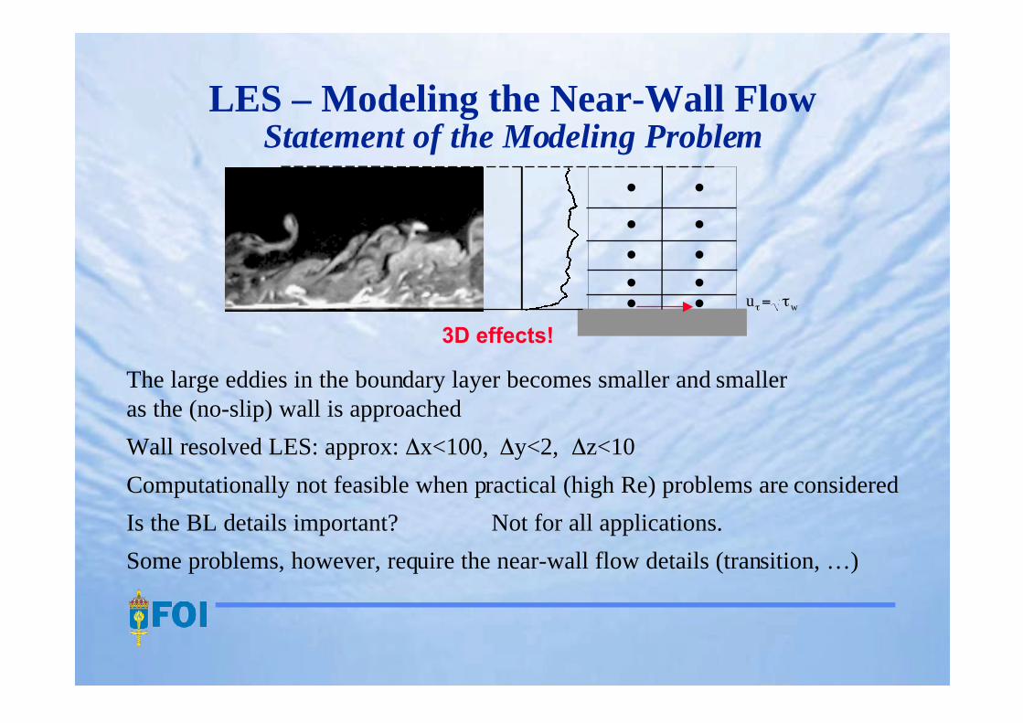
LES – Modeling the Near-Wall FlowStatement of the Modeling Problem

The large eddies in the boundary layer becomes smaller and smalleras the (no-slip) wall is approached

Wall resolved LES: approx: ∆x<100, ∆y<2, ∆z<10

Computationally not feasible when practical (high Re) problems are considered

Is the BL details important? Not for all applications.

Some problems, however, require the near-wall flow details (transition, …)

•

u wτ τ=•

3D effects!

•

•

••

••

•

•

LES – Modeling the Near-Wall FlowTraditional Wall Handling

Traditional SGS model improvementsDamping function (e.g. van Driest)Necessary to damp νk when flow not properly resolvedDoes no aleviate resolution requirement

Dynamic SGS model coefficient estimationcD, ck captures the behaviour when y→0Unclear what happens in practical problems

Traditional Wall-ModelingRelate ττττw to the tangential velocity components usingthe law of the wall(Deardorff, Grözbach, Schumann, …)

Zonal ApproachNumerical solution of BL equations on a secondarybeween LES grid and wall(Balaras et al.)

• •3D effects!

• •

u wτ τ=• •

3D effects!

νk y∝ 3

LES – Modeling the Near-Wall FlowWall-Models

For geometrically complex high Re number flows the traditional modelsare difficult to implement and are found to give poor results

Hypothesis: Can we adjust the eddy viscosity (parameter) to satisfy the log-law? Streaks as frequent as hairpin vortices in free flows Incorporate the effects of the unresolved flow by means of νk

Model: Determine (locally) uτ from

and modify the effecive viscosity according to

( ) /( / ) /, , ,ν ν τ ∂ ∂ τ+ ≡ = +BC P w y P P y P y Pv y u y v

vy p y p y B

y p B y p y B

yu i

yu i

y

yu i

yu i

y+

+ + +

+ + +=

+ −( )− − <

+ + + −( )− − >

+ + +

+ + +

+ if

if

ν νκ κ

κνκ

νκ κ

τ τ

τ τ

∂ ∂

∂ ∂

( ) ( ) ( ) ln| |

ln| | ( ) ( ) ln| |

2

3 3

3

2 21 1

12

1 1

0

0

uu

y u y v v uwτ

τ τ

τ ν

ν

= = ∇

= =+ +

| (( ) )|

( / ) , /

v t

Turbulent Channel Flow Reττττ=590-1800

100

102

0

10

20

30

40

50

<v x>

/uta

u

y+

DNS/EXPMIXED+WMMIXED+van-Driest

Mean velocity

100

102

0

2

4

6

8

10

v rms/u

tau

y+

DNS/EXPMIXED+WMMIXED+van-Driest

Rms velocity

0 0.2 0.4 0.6 0.8 1-3

-2.5

-2

-1.5

-1

-0.5

0

Rxy

/uta

u2

y/h

DNS/EXPMIXED+WMMIXED+van-Driest

Shear stress

Reτ=395, 595, 1800 and 10,000DNS: Moin, Kim & MoserEXP: Wei & Willmarth603 grid∆x+=[40 0.3 20] to [1000 11 500]

-0.05 -0.025 0 0.025 0.05

-0.025

-0.0125

0

0.0125

0.025

-0.05 -0.025 0 0.025 0.05

-0.025

-0.0125

0

0.0125

0.025

-0.05 -0.025 0 0.025 0.05

-0.025

-0.0125

0

0.0125

0.025

-0.2 -0.1 0 0.1 0.2

-0.05

-0.025

0

0.025

0.05

-0.2 -0.1 0 0.1 0.2

-0.05

-0.025

0

0.025

0.05

-0.2 -0.1 0 0.1 0.2

-0.05

-0.025

0

0.025

0.05

Velocity PDFs in BL

sweep (Q2: –u´, +w´)ejection (Q4: +u´, –w´)

The larger extent of the PDFs at y+=20 and 40indicates the low-speed streak lift-up bursting

u

||D||2–||W||2<0

vx

~2400·l

~1000·llow speedstreak

high speed streak

LES @ Reττττ=395

w

Re=395

Re=1800

Turbulent Channel Flow Reττττ=590-1800

Detatched Eddy Simulation (DES)Consider the incompressible NSE

The NSE are formally filtered in order to remove the attached eddies

Closure required for B (as for LES)

with

Here,

The basic idea is to use the advantage of some RANS turbulence

models (e.g. the Spalart-Allmares model) to handle the near-wallturbulence modeling. When ∆>δ99 LES is used!

∇⋅ =

+∇⋅ =−∇ +∇⋅ − + + ⊗

( )

( ) ( ) ( )

v

v v v S B f m

m

pt∂

B B B I DD vtr f= − =−13 12( ) ( ˜ )ν

∂ ν ν ν ν ν σ ν σ ν νt b b w wc S c c f d(˜ ) ( ˜ ) ˜ ˜ ([( ˜ )/ ] ˜ ) ( / )( ˜ ) ( ˜ / ˜ )+∇⋅ = +∇⋅ + ∇ + ∇ −v 1 22

12

∆= ∆ ∆ ∆max( , , )x y z

LES

RANS

RANS, DES and LESFlow around a circular cylinder @ Re=3900

Complexapplications

DES

From Nikitin & Spalart

Two-Level Simulation Models (Menon et al)Both the resolved and subgrid scales of motion are explicitly simulated

where

In TLS v´ is modeled as a family of 1D vector-fieldsembedded in the LES grid

• the 1D lines extend over the entire domain

• turbulent stirring modeled using the triplet map

• built-in wall handling

• extension of the ODT of Kerstein, 1999

• modeling by dimension reduction

∇⋅ =

+∇⋅ =−∇ +∇⋅ −∇⋅ ⊗

v

v v v S B

0

∂ t p( ) ( )

∇⋅ ′=

′ +∇⋅ ′ ′ =−∇ ′+∇⋅ ∇ ′ +∇⋅ − ′− ′ ⊗ ⊗ ⊗

v

v v v v B v v v v

0

∂ νt p( ) ( ) ( ) ( )

B v v v v v v v v v v= − + ′+ ′ + ′ ′⊗ ⊗ ⊗ ⊗ ⊗( ) ( ) ( )

GS

SGS

no−slip wall

LES cells

ODT Lines

z

x

U

W

Homogenization-based LESHomogenization by multiple scales expansion

gives

Linearity and superposition

Approach 1: Numerical simulation (χ or v1) using grid-within-the-grid approach

Approach 2: Analytical (no transport, w related to a k–5/3 spectra)

Stochastic process

∂ +∇ ⋅ =−∇ +∇ ⋅ ∇ −

∂ +∇ ⋅ + =−∇ + ∇ −∇ ⋅= +

⊗

⊗ ⊗ ⊗⊗ ⊗

t x x x x

x

p

p

v v v v B

v w v v w v w vB v w w v

( ) ( )

( ) ˜ ( );

ν

ντ ξ ξ ξ1 1 12

11 1

v v v v x v x v v v w= + ′ = +∑ + ′ = + ++=∞ −

δ δ δδ τ τ δ δ( , ) ( , ; , ) ( , )t tkkk ξξ ξξ1 1

1

B w w v A viji

klj j

kli

x

kijkl x

kl l= + ∂ = ∂( )χ χ

∂ +∂ + = ∇ −τ ξ ξχ χ χ ν χ δklj m

klj

klm j

klj

kj l

m w w w( ) 2

A Ahjklc c k

hjklk= ε

π ν

2 3 2

11 32

/

/( )˜ ( )∆ ∆∆

The ‘microstructure problem’

100

102

0

10

20

30

40

50<

v x>/u

tau

y+

DNS/EXPDSMGMIXED+WMMIXED+van-DriestOEEVM+WMMILES+WMDESTLS

Mean velocity

100

102

0

2

4

6

8

10

v rms/u

tau

y+

DNS/EXPDSMGMIXED+WMMIXED+van-DriestOEEVM+WMMILES+WMDESTLS

Rms velocity

0 0.2 0.4 0.6 0.8 1-3

-2.5

-2

-1.5

-1

-0.5

0

Rxy

/uta

u2

y/h

DNS/EXPDSMGMIXED+WMMIXED+van-DriestOEEVM+WMMILES+WMDESTLS

Shear stress

Turbulent Channel Flow Reττττ=590-1800

Flow around a !!!! Cylinder

Key issues is to handlethe free separation

||∇v||2 ||∇×v||2

Classical validation problem for LES (and RANS)ReD=3900DNS: Beudan & Moin, Tremblay et al., EXP: Lourenco & Shih and Ong & WallaceGrid: ~ 500,000 to 1,300,000 hex/tet (y+≈10)20D downstream

Re=3900

Re=140000

ΘΘΘΘ≈≈≈≈120°

ΘΘΘΘ≈≈≈≈90°

Flow around a !!!! Cylinder

Flow around a !!!! Cylinder, Re=3900

-4 -2 0 2 4

0

1

2

3

4

5

6

7

<v x>

/v0

y/D

Lourenco & ShihOng & WallaceMM+WMOEEVM+WMMILES+WMRANS RSM

-3 -2 -1 0 1 2 30

0.5

1

1.5

2

(vxrm

s )2 /v02

y/D

Lourenco & ShihOng & WallaceMM+WMOEEVM+WMMILES+WM

Rms velocity fluctuationMean velocity

Good agreement for all LES models– well resolved LES (y+≈10)– wake recovery very well predictedRANS (k-ε and RSM) not that accurate

0 1 2 3 4 5 6−2

−1.5

−1

−0.5

0

0.5

1

1.5

2

c P

phi

Norberg Re=3000MM+WMOEEVM+WMMILES+WMRANS k−epsRANS RSM

Cp

-4 -2 0 2 4

0

1

2

3

4

5

6<

v x>/v

0

y/D

Cantwell & ColesMM+WMOEEVM+WMMILES+WMRANS RSM

Flow around a !!!! Cylinder, Re=140,000

-4 -2 0 2 4

0

0.1

0.2

0.3

0.4

0.5

0.6

0.7

(vxrm

s )2 /v02

y/D

Cantwell & ColesMM+WMOEEVM+WMMILES+WM

Rms velocity fluctuationMean velocity

Reasonable agreement for all LES models– marginally resolved LES (y+≈10 but not sufficient resolution in spanwise direction)– too large recirculation bubbleRANS (k-ε and RSM) not that accurate

Flow around a 6:1 Prolate Spheroid

x/L=0.600

x/L=0.772k U

k U

LDKM, αααα=20°°°°

primaryseparation

secondaryseparation

RANS: Tsai et al., 1999, AIAA 99-0172DES: Constantinescu et al., 2002, AIAA 02-0588LES: Wikström et al., 2004, JoT, 5, p 29

measurementsections

Flow around a 6:1 Prolate Spheroid

0 0.2 0.4 0.6 0.8 1−0.5

0

0.5

1

x/L

Cp

OEEVM+WMOEEVM+WMOEEVMLDKMOEEVM+WM fine gridEXP 10EXP 20

CP @ meridian plane

0 0.002 0.004 0.006 0.008 0.01 0.012 0.014 0.016−0.6

−0.4

−0.2

0

0.2

0.4

0.6

0.8

1

y

U/v

0, V/v

0, W/v

0

U/v0 @ ϕϕϕϕ=90°°°°, x/L=0.600

U/v0

V/v0

W/v0

Surface Mounted Bump

Experiments by:Simpson, Long & Byun, 2002U=27.5 m/sRe=1.3·105

δ99=H/2Analytical hill profile

LES: MIXED+WM

EXP: OIL FLOW

Surface streamlines

2H

6H

Surface Mounted Bump

⟨⟨⟨⟨p⟩⟩⟩⟩

Submarine Hydrodynamics

DARPA SUBOFF AFF-8DTMB wind tunnel modelscale 1:24L=4.36 mD=0.51 mv0=44 m/sRe=12 ·106

Grids: 2.5, 5 & 10 millionHorseshoe vortex

thin separation

Submarine Hydrodynamics

0 0.5 10

0.2

0.4

0.6

0.8

1

v/v0

r/r m

idsh

ip

0 0.5 10

0.2

0.4

0.6

0.8

1

v/v0

r/r m

idsh

ip0 0.5 1

0

0.2

0.4

0.6

0.8

1

v/v0

r/r m

idsh

ip

0 0.5 10

0.2

0.4

0.6

0.8

1

v/v0

r/r m

idsh

ip

0 0.5 10

0.2

0.4

0.6

0.8

1

v/v0

r/r m

idsh

ip

OEEVMMMOEEVM fine gridMM fine gridEXP DTMB AFF−1

Bare hull configuration(2.0, 4.0 and 8.0 M cells)• Geometry of wind tunnel

• trip-wire at the bow• inflow turbulence• model insufficiencies

0 0.2 0.4 0.6 0.8 1-1

-0.5

0

0.5

1

CP

x/L

LES OEEVM+WMLES MM+WMEXP DTMB AFF8

0 0.2 0.4 0.6 0.8 10

0.5

1

1.5

2

2.5

3

3.5

4r/

r mid

ship

v/v0

AFF8 LES OEEVM+WMAFF8 LES MM+WMAFF1 LES OEEVM+WMAFF1 LES MM+WMEXP AFF1 (bare hull)EXP AFF8 (hull+sail+rudders)

0 0.02 0.04 0.06 0.08 0.10

0.5

1

1.5

2

2.5

3

3.5

4

r/D

vrms/v0

AFF8 LES OEEVM+WMAFF8 LES MM+WMEXP AFF1 (bare hull)

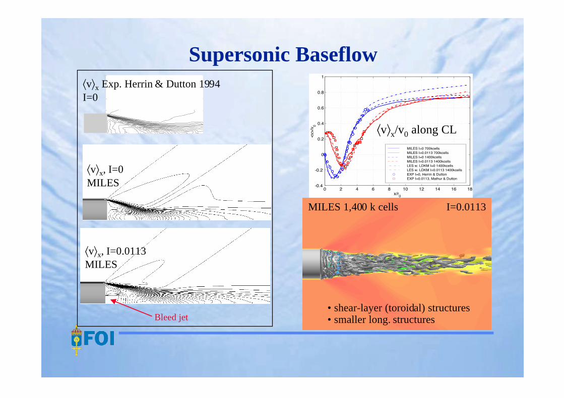
Supersonic Baseflow

1,400k and 2,800k mesh

OEEVM and MILES

fixed inlet (Blasius) profile

exp. of Dutton et al (1994, …)

Re=2.86·106

Ma=2.46

p p T T= = =0 0 0, , v v

∇ = ∇ ⋅ = ∇ =p T0 0, , v n 0

0 0.2 0.4 0.6 0.8 10

0.2

0.4

0.6

0.8

1

<v>/v0

r/r 0

inlet (Blasius) profile

Supersonic Baseflow

0 2 4 6 8 10 12 14 16 18-0.4

-0.2

0

0.2

0.4

0.6

0.8

1

x/r0

<v>/

v 0

MILES I=0 700kcellsMILES I=0.0113 700kcellsMILES I=0 1400kcellsMILES I=0.0113 1400kcellsLES w. LDKM I=0 1400kcellsLES w. LDKM I=0.0113 1400kcellsEXP I=0, Herrin & DuttonEXP I=0.0113, Mathur & Dutton

⟨v⟩x/v0 along CL

MILES 1,400 k cells I=0.0113

• shear-layer (toroidal) structures• smaller long. structures

⟨v⟩x, I=0.0113MILES

Bleed jet

⟨v⟩x Exp. Herrin & Dutton 1994I=0

⟨v⟩x, I=0MILES

Concluding RemarksLES appars to do a better job than expected for high Re wall bounded flows

LES better but much more expensive

Subgrid wall models required

Difficult to bridge the gap between simple and complex flows

Need for high-quality high Re exp. data

Inflow/outflow BC charactrization

Inflow/outflow BC modeling

Considerable room for improvement w.r.t. SGS modeling