In J. Keller and Z. Oziewicz (Eds.), The Theory of the Electron,UNAM, Facultad de Estudios Superiores, Cuautitlan, Mexico (1996), p. 1–50.

REAL DIRAC THEORY

David HestenesDepartment of Physics & Astronomy

Arizona State UniversityTempe, AZ 85287

Abstract

The Dirac theory is completely reformulated in terms of Spacetime Algebra, a real Clifford Algebra char-

acterizing the geometrical properties of spacetime. This eliminates redundancy in the conventional matrix

formulation and reveals a hidden geometric structure in the theory. Among other things, it reveals that

complex numbers in the Dirac equation have a kinematical interpretation, with the unit imaginary identi-

fied as the generator of rotations in a spacelike plane representing the direction of electron spin. Thus, spin

and complex numbers are shown to be inextricably related in the Dirac Theory. This leads to a new version

of the zitterbewegung, wherein local circular motion of the electron is directly associated with the phase

factor of the wave function. In consequence, the electron spin and magnetic moment can be attributed to

the zitterbewegung, and many other features of quantum mechanics can be explained as zitterbewegung

resonances.

INTRODUCTION.

This paper reviews and consolidates results from a line of research1–14 aimed at clarifyingthe Dirac electron theory and simplifying its mathematical formulation. The central resultis a representation of the Dirac wave function which reveals geometric structure in theDirac theory — structure which is not at all apparent in the conventional formulation.Besides computational benefits, this result has many implications for the interpretation ofquantum mechanics, ranging from the classical limit to possibilities of a substructure in theDirac theory. Before we can address these issues, however, an analysis and revision of theunderlying mathematical formalism is needed.

Most physicists regard the Dirac algebra as the algebra of a relativistic spin- 12 particle.

However, there is a broader interpretation with far-reaching consequences. Dirac’s gammamatrices can be regarded as representations of spacetime vectors. These vectors generate areal Clifford algebra, which has been dubbed the Spacetime Algebra (STA), because it pro-vides a complete, nonredundant characterization of the metrical and directional propertiesof spacetime. All the elements of the STA have straightforward geometric interpretations.This brings to light a geometric significance of the Dirac algebra which was implicit inDirac’s original formulation but only dimly recognized since. Since STA is a universal alge-bra of spacetime properties, it is more than a special tool for characterizing spin- 1

2 particles.It is equally applicable to every domain of classical and quantum physics.

Reformulation of the Dirac Theory in terms of STA reveals that the conventional matrixformulation contains superfluous degrees of freedom in its use of complex numbers. This

1

redundancy is eliminated in the STA formulation wherein the base number field is realrather than complex. Its most immediate and striking consequence is a revelation of thegeometrical role played by complex numbers in the Dirac Theory. It reveals that the unitimaginary appearing in the Dirac equation and the energy-momentum operators representsthe bivector generator of rotations in a spacelike plane corresponding to the direction ofelectron spin. In other words, the factor ih represents spin in the Dirac theory—the irepresents the spin direction while h/2 is the magnitude of the spin. It must be emphasizedthat this is not an adventitious interpretation of h arbitrarily imposed on the Dirac theory.It has been implicit in the theory from the beginning. The STA formulation only makes itexplicit.

In as much as complex wave functions clearly play a crucial role in quantum mechan-ics, the discovery that the ubiquitous factor ih is inextricably associated with spin in theDirac theory must surely be a critical clue to a deeper interpretation of quantum mechan-ics. Its implications are not immediately obvious, however, and they evidently cannot beunderstood apart from a thorough analysis of the Dirac theory. The approach reviewed inthis paper is to systematically study the geometric structure of the Dirac equation and itssolutions as revealed by the STA formulation. The geometric structure of the Dirac theoryis taken to be the most reliable guide to its physical interpretation as well as to feasiblemodifications and extensions.

The central result is an invariant decomposition of the Dirac wave function into a 2-parameter statistical factor and a 6-parameter kinematical factor. Among its implicationsare the following: The statistical factor characterizes the admixture of electron-positronstates without employing Fourier analysis. The kinematical factor admits a kinematicalinterpretation of the complex phase factor and relates it to the spin. The fullest interpre-tation is achieved by a simple change in identification of the electron velocity which revealsa zitterbewegung substructure inherent in the Dirac theory. This opens up possibilities forprobing the substructure experimentally. Other possibilities arise from noting that theinvariance group of the Dirac current has the structure of the electroweak gauge group.

In two appendixes the coupled Dirac-Maxwell field equations are derived from a La-grangian and the associated conservation laws are derived from Poincare invariance.

This article was originally prepared in 1990 and circulated as a preprint. The wholeapproach has been further elaborated along several lines since.37–46 References 45 and 46are especially noteworthy because they present a number of physical applications, includingtunneling, electron diffraction and Stern-Gerlach splitting, with new insights into each ofthem.

1. SPACETIME ALGEBRA AND CALCULUS.

We shall employ a flat space model of the physical spacetime manifold in this article, soeach point event can be represented by a unique element x in a real 4-dimensional vectorspace M4. The properties of scalar multiplication and vector addition in M4 provideonly a partial characterization of spacetime geometry. To complete the characterizationwe introduce an associative geometric product among vectors with the property that thesquare x2 of any vector x is a (real) scalar. As usual, we say that the vector x is timelike,lightlike or spacelike if x2 > 0, x2 = 0, x2 < 0 respectively.

2

The vector spaceM4 is not closed under the geometric product. Rather, by multiplicationand addition it generates a real associative (but noncommutative) algebra of dimension24 = 16, commonly called the Geometric Algebra (or Clifford Algebra) of M4. We call itthe spacetime algebra (STA), because all its elements and operations represent geometricelements and relations, and it suffices for the representation of any geometric structure onspacetime.

To facilitate applications of STA to physics it is necessary to build a system of definitionsand theorems. From the geometric product uv of two vectors it is convenient to define twoother products. The inner product u · v is defined by

u · v = 12 (uv + vu) = v · u , (1.1)

while the outer product u ∧ v is defined by

u ∧ v = 12 (uv − vu) = v ∧ u . (1.2)

The three products are therefore related by

uv = u · v + u ∧ v , (1.3)

and this can be regarded as a decomposition of the product uv into symmetric and skewsym-metric parts.

The inner and outer products can be generalized. We define the outer product along withthe notion of k-vector iteratively as follows: Scalars are defined to be 0-vectors, vectors are1-vectors, and bivectors, such as u∧ v, are 2-vectors. For a given k-vector K, the integer kis called the step (or grade) of K. For k ≥ 1, the outer product of a vector v with a k-vectorK is a (k + 1)-vector defined in terms of the geometric product by

v ∧K = 12 (vK + (−1)kKv) = (−1)kK ∧ v . (1.4)

The corresponding inner product is defined by

v ·K = 12 (vK + (−1)k+1Kv) = (−1)k+1K · v , (1.5)

and it can be proved that the result is a (k − 1)-vector. Adding (1.4) and (1.5) we obtain

vK = v ·K + v ∧K , (1.6)

which obviously generalize (1.3). The important thing about (1.6), is that it decomposesvK into (k − 1)-vector and (k + 1)-vector parts.

By continuing as above, the STA as been developed into a complete coordinate-freecalculus for spacetime physics. However, to hasten comparison with standard Dirac the-ory, we interrupt that process to introduce coordinates and a basis for the algebra. Letγµ; 0, 1, 2, 3 be a right-handed orthonormal frame of vectors with γ0 in the forward lightcone. In accordance with (1.1), the components gµν of the metric tensor for this frame aregiven by

gµν = γµ · γν = 12 (γµγν + γνγµ) . (1.7)

3

The unit pseudoscalar i for spacetime is related to such a frame by the equation

i = γ0γ1γ2γ3 = γ0 ∧ γ1 ∧ γ2 ∧ γ3 . (1.8)

It is readily verified from (1.8) that i2 = −1, and the geometric product of i with any vectoris anticommutative. Hereafter it will be convenient to refer to γµ as a standard frame.

For manipulating coordinates it is convenient to introduce the reciprocal frame γµdefined by the equations

γµ = gµνγν or γµ · γν = δνµ . (1.9)

(Summation convention in force!) The relation of scalar coordinates xµ to the spacetimepoint x they designate is then given by

xµ = γµ · x and x = xµγµ . (1.10)

By multiplication the γµ generate a complete basis of k-vectors for STA, consisting of the24 = 16 linearly independent elements

1, γµ, γµ ∧ γν , γµi, i . (1.11)

Any multivector can be expressed as a linear combination of these elements. For example,a bivector F has the expansion

F = 12F

µνγµ ∧ γν , (1.12a)

with its “scalar components” Fµν given by

Fµν = γµ · F · γν = γµ · (γν · F ) = (γµ ∧ γν) · F . (1.12b)

Note that the two inner products in the middle term can be performed in either order, soa parenthesis is not needed.

The entire spacetime algebra is obtained by taking linear combinations of basis k-vectorsin (1.11) obtained by outer multiplication of vectors in M4. A generic element M of theSTA, called a multivector, can thus be written in the expanded form

M = α+ a+ F + bi+ βi , (1.13)

where α and β are scalars, a and b are vectors, and F is a bivector. This is a decompositionof M into its k-vector parts, with k = 0, 1, 2, 3, 4, as is expressed more explicitly by puttingit in the form

M =

4∑k=0

M(k) (1.13′)

where the subscript (k) means “k-vector part.” Of course, M(0) = α, M(1) = a, M(2) = F ,M(3) = bi, M(4) = βi

Computations are facilitated by the operation of reversion. For M in the expanded form(1.13) the reverse M can be defined by

M = α+ a− F − bi+ βi . (1.14)

4

Note, in particular, the effect of reversion on the various k-vector parts.

α = α, a = a, F = −F, i = i .

It is not difficult to prove that(MN)˜ = NM , (1.15)

for arbitrary multivectors M and N .Any multivector M can be decomposed into the sum of an even part M+ and an odd

part M− defined in terms of the expanded form (1.13) by

M+ = α+ F + βi , (1.16a)

M− = a+ bi , (1.16b)

or, equivalently, byM± = 1

2 (M ∓ iMi) . (1.16c)

The set M+ of all even multivectors forms an important subalgebra of STA called theeven subalgebra.

We are now in position to describe the relation of STA to the Dirac algebra. The Diracmatrices are representations of the vectors γµ by 4×4 matrices, and we emphasize this cor-respondence by denoting the vectors with the same symbols γµ ordinarily used to representthe Dirac matrices. In view of what we know about STA, this correspondence reveals thephysical significance of the Dirac matrices, appearing so mysteriously in relativistic quan-tum mechanics: The Dirac matrices are no more and no less than matrix representations ofan orthonormal frame of spacetime vectors and thereby they characterize spacetime geom-etry. But how can this be? Dirac never said any such thing! And physicists today regardthe set γµ as a single vector with matrices for components. Nevertheless, their practiceshows that the “frame interpretation” is the correct one, though we shall see later thatthe “component interpretation” is actually equivalent to it in certain circumstances. Thecorrect interpretation was actually inherent in Dirac’s argument to derive the matrices inthe first place: First he put the γµ in one-to-one correspondence with orthogonal directionsin spacetime by indexing them. Second, he related the γµ to the metric tensor by imposingthe “peculiar condition” (1.7) on the matrices for formal algebraic reasons. But we haveseen that this condition has a clear geometric meaning in STA, a meaning which demandsthe “frame interpretation” though it is compatible with the “component interpretation.”Finally, Dirac introduced associativity automatically by employing matrix algebra, with-out realizing that it has a geometric meaning. The geometric meaning of associativity ingeometric algebra is discussed at length in Chap. 1 of Ref. 16.

If indeed the physical significance of the Dirac matrices derives entirely from their inter-pretation as a frame of vectors, then their specific matrix properties must be irrelevant tophysics. We shall prove this by dispensing with matrices altogether and formulating theDirac theory entirely in terms of STA. A step in this direction has already been taken inconventional approaches by proving that physical predictions are invariant under a changeof matrix representation. Though the particular representation is irrelevant, it is requiredthat γ0 be hermitian while the γk are antihermitian, as expressed by

γ0† = γ0 , γk

† = −γk . (1.17)

5

Though hermitian conjugation is a matrix operation, it has a representation in STA thatgives it a physical meaning. For any multivector M , we define the hermitian conjugate by

M† = γ0Mγ0 . (1.18)

Clearly, this is not an invariant operation because it depends on the selection of a particulartimelike direction. Its physical significance will be made clear in the next Section.

Finally, we note that the Dirac algebra is the matrix algebra generated by the Diracmatrices over the base field of the complex numbers. Let i′ =

√−1 denote the unit imagi-

nary in the base number field. In contrast to the γµ, i′ does not represent any property ofspacetime. Furthermore, STA already contains a number of “geometrical roots” of minusone, including

γ2k = −1, (γ2γ1)2 = −1, i2 = (γ0γ1γ2γ3) = −1 .

We shall see that these roots can take over the role of i′ in the Dirac theory, therebyrevealing its geometrical meaning. Note that the complex base field gives the Dirac algebratwice as many degrees of freedom as STA. Evidently these 16 additional degrees of freedomare devoid of geometrical or physical significance, serving only to obscure the geometriccontent of the algebra. For these reasons we stick with STA and eschew the Dirac algebrauntil we need it for translating the matrix version of the Dirac theory into STA.

With STA we can describe physical processes by equations which are invariant in the sensethat they are not referred to any inertial system. However, observations and measurementsare usually expressed in terms of variables tied to a particular inertial system, so we needto know how to reformulate invariant equations in terms of those variables. STA providesa very simple way to do that called a space-time split.

In STA a given inertial system is completely characterized by a single future-pointing,timelike unit vector. Refer to the inertial system characterized by the vector γ0 as the γ0-system. The vector γ0 is tangent to the world line of an observer at rest in the γ0-system,so it is convenient to use γ0 as a name for the observer. The observer γ0 is representedalgebraically in STA in the same way as any other physical system, and the spacetime splitamounts to no more than comparing the motion of a given system (the observer) to otherphysical systems.

An inertial observer γ0 determines a unique mapping of spacetime into the even subalgebraof STA. For each spacetime point (or event) x the mapping is specified by

xγ0 = t+ x , (1.19a)

wheret = x · γ0 (1.19b)

andx = x ∧ γ0 . (1.19c)

This defines the γ0-split of spacetime. In “relativistic units” where the speed of light c = 1,t is the time parameter for the γ0-system. Equation (1.19b) assigns a unique time t to everyevent x; indeed, (1.19b) is the equation for a one parameter family of spacelike hyperplaneswith normal γ0.

6

The set of all position vectors (1.19c) is the 3-dimensional position space of the observerγ0, which we designate by P3 = P3(γ0) = x = x ∧ γ0. Note that P3 consists of allbivectors in STA with γ0 as a common factor. In agreement with common parlance, werefer to the elements of P3 as vectors. Thus, we have two kinds of vectors, those in M4

and those in P3. To distinguish between them, we may refer to elements of M4 as propervectors and to elements of P3 as relative vectors (relative to γ0, of course!). Also, relativevectors will be designated in boldface.

By the geometric product and sum the vectors in P3 generate the entire even subalgebraof STA as the geometric algebra of P3. This is made obvious by constructing a basis.Corresponding to a standard basis γµ forM4, we have a standard basis σk; k = 1, 2, 3for P3, where

σk = γk ∧ γ0 = γkγ0 . (1.20a)

These generate a basis for the relative bivectors:

σi ∧ σj = σiσj = iσk = γjγi , (1.20b)

where the allowed values of the indices i, j, k are cyclic permutations of 1,2,3. The rightsides of (1.20) and (2.5) show how the bivectors for spacetime are split into vectors andbivectors for P3. Remarkably, the right-handed pseudoscalar for P3 is identical to that forM4; thus,

σ1σ2σ3 = i = γ0γ1γ2γ3 . (1.20c)

It will be noted that the geometric algebra of P3 is isomorphic to the Pauli algebra,with the σk corresponding to the 2× 2 Pauli matrices. However, if the γµ are regarded asDirac matrices, then (1.20) defines 4× 4 matrix representations of the σk; these are the αkmatrices of Dirac.7 This awkward distinction between 2×2 and 4×4 matrix representationsis another unnecessary complication in the conventional formulation of quantum mechanics.It is entirely irrelevant to the simple relation between relative and proper basis vectorsdefined by (1.20a).

To complete the correspondence with matrix representations, consider hermitian conju-gation again. According to the definition (1.18), the σk are hermitian, that is,

σ†k = σk and (σiσj)† = σjσi . (1.21)

But this defines the geometrical operation of reversion in the algebra of P3. Thus, hermitianconjugation has the geometrical meaning of reversion “in” an inertial system.

Let x = x(τ) be the history of a particle with proper time τ and proper velocity v = dx/dt.The space-time split of v is obtained by differentiating (1.19a); whence

vγ0 = v0(1 + v) , (1.22a)

where

v0 = v · γ0 =dt

dτ=(1− v2

)− 12 (1.22b)

is the “time dilation” factor, and

v =dx

dt=dτ

dt

dx

dτ=v ∧ γ0

v · γ0(1.22c)

7

is the relative velocity in the γ0-system. The last equality in (1.22b) was obtained from

1 = v2 = (vγ0)(γ0v) = v0(1 + v)v0(1− v) = v20(1− v2) .

An electromagnetic field is a bivector-valued function F = F (x) on spacetime. Anobserver γ0 splits it into an electric (relative vector) part E and, a magnetic (relativebivector) part iB; thus

F = E + iB , (1.23a)

whereE = (F · γ0)γ0 = 1

2 (F + F †) , (1.23b)

iB = (F ∧ γ0)γ0 = 12 (F − F †) , (1.23c)

and, in accordance with (1.18), F † = E− iB. Equation (1.23a) represents the field formallyas a complex (relative) vector; but it must be remembered that the imaginary i here is theunit pseudoscalar and so has a definite geometric meaning. Indeed, (1.23a) shows that themagnetic field is actually a bivector quantity iB, and its conventional representation asa vector B is a historical accident in which the duality is hidden in the notion of “axialvector.”18,16

At this point it is worth noting that the geometric product of relative vectors E andB can be decomposed into symmetric and antisymmetric parts in the same way that wedecomposed the product of proper vectors. Thus, we obtain

EB = E ·B = i(E××B) , (1.24a)

whereE ·B = 1

2 (EB + BE) (1.24b)

is the usual dot product for Euclidean 3-space, and

E××B =1

2i(EB−BE) = i−1(E ∧B) (1.24c)

is usual cross product of Gibbs. Thus, the standard vector algebra of Gibbs is smoothlyimbedded in STA and simply related to invariant spacetime relations by a spacetime split.Consequently, translations from STA to vector algebra are effortless. Moreover, the com-bination (1.24) of the dot and cross products into the single geometric product simplifiesmany aspects of classical nonrelativistic physics, as demonstrated at length in Ref. 16.

In terms of spacetime coordinates defined by (1.10), an operator 5 interpreted as thederivative with respect to a spacetime point x can be defined by

5 = γµ∂µ (1.25)

where

∂µ =∂

∂xµ= γµ ·5 . (1.26)

The square of is the d’Alembertian

52= gµν∂µ∂ν . (1.27)

8

The matrix representation of (1.25) will be recognized as the “Dirac Operator,” originally

discovered by Dirac by seeking a “square root” of 52in order to find a first order relativis-

tically invariant wave equation, the famous “Dirac equation” discussed in the next Section.However, in STA where the γµ are vectors, it is clear that 5 is a vector operator, becauseit is the derivative with respect to a vector representing a spacetime point. Contrary tothe impression given by conventional accounts of relativistic quantum theory, 5 is not anoperator specially adapted to spin-1/2 wave equations. Here we show that it is equally aptfor electromagnetic field equations.

In STA an electromagnetic field is represented by a bivector-valued function F = F (x)on spacetime. The field produced by a source with spacetime current density J = J(x) isdetermined by Maxwell’s Equation

5F = J . (1.28)

Using (1.11) again to write5F = 5 · F +5∧ F , (1.29)

(1.28) can be separated into a vector part

5 · F = J (1.30a)

and a trivector part5∧ F = 0 . (1.30b)

Expressed in terms of a basis by using (1.25) and (1.12a), these two equations are seen toas equivalent to the usual tensor form of Maxwell’s equations.

Sometimes the source current J can be decomposed into a conduction current JC and amagnetization current 5 ·M , where the generalized magnetization M = M(x) is a bivectorfield; thus

J = JC +5 ·M . (1.31)

The Gordon decomposition of the Dirac current is of this ilk. Because of the mathematicalidentity 5 · (5 ·M) = (5 ∧5) ·M = 0, the conservation law 5 · J = 0 implies also that5 · JC = 0. Using (1.31), equation (1.30a) can be put in the form

5 ·G = JC (1.32)

where we have defined a new field

G = F −M . (1.33)

A disadvantage of this approach is that it mixes up physically different kinds of entities, anE-M field F and a matter field M . However, in most materials M is a function of the fieldF , so when a “constitutive equation” M = M(F ) is known (1.32) becomes a well definedequation for F .

STA enables us to write the usual Maxwell energy-momentum tensor T (n) = T (n(x), x)for the electromagnetic field in the compact form

T (n) = 12FnF = −1

2FnF . (1.34)

9

Recall that the tensor field T (n) is a vector-valued linear function on the tangent spaceat each spacetime point x describing the flow of energy-momentum through a surface withnormal n = n(x), By linearity T (n) = nµT

µ, where nµ = n · γµ and

Tµ ≡ T (γµ) = 12Fγ

µF . (1.35)

The divergence of T (n) can be evaluated by using Maxwell’s equation (1.28), with the result

∂µTµ = T (5) = J · F . (1.36)

Its value is the negative of the Lorentz Force F · J , which is the rate of energy-momentumtransfer from the source J to the field F .

2. THE REAL DIRAC EQUATION

To find a representation of the Dirac theory in terms of the STA, we begin with a Diracspinor Ψ, a column matrix of 4 complex numbers. Let u be a fixed spinor with the properties

u†u = 1 , (2.1a)

γ0u = u , (2.1b)

γ2γ1u = i′u . (2.1c)

In writing this we regard the γµ, for the time being, as 4× 4 Dirac matrices, and i′ as theunit imaginary in the complex number field of the Dirac algebra. Now, we can write anyDirac spinor

Ψ = ψu , (2.2)

where Ψ is a matrix which can be expressed as a polynomial in the γµ. The coefficients inthis polynomial can be taken as real, for if there is a term with an imaginary coefficient,then (2.1c) enables us to make it real without altering (2.2) by replacing i′ in the term byγ2γ1 on the right of the term. Furthermore, the polynomial can be taken to be an evenmultivector, for if any term is odd, then (2.1b) allows us to make it even by multiplyingon the right by γ0. Thus, in (2.2) we may assume that ψ is a real even multivector. Nowwe may reinterpret the γµ in ψ as vectors in the STA instead of matrices. Thus, we haveestablished a correspondence between Dirac spinors and even multivectors in the STA. Thecorrespondence must be one-to-one, because the space of even multivectors (like the spaceof Dirac spinors) is exactly 8-dimensional, with 1 scalar, 1 pseudoscalar and 6 bivectordimensions.

There are other ways to represent a Dirac spinor in the STA,12 but all representations are,of course, mathematically equivalent. The representation chosen here has the advantagesof simplicity and, as we shall see, ease of interpretation.

To distinguish a spinor ψ in the STA from its matrix representation Ψ in the Dirac alge-bra, let us call it a real spinor to emphasize the elimination of the ungeometrical imaginaryi′. Alternatively, we might refer to ψ as the operator representation of a Dirac spinor,because, as shown below, it plays the role of an operator generating observables in thetheory.

10

In terms of the real wave function ψ, the Dirac equation for an electron can be writtenin the form

γµ(∂µψγ2γ1h− eAµψ) = mψγ0 , (2.3)

where m is the mass and e = −| e | is the charge of the electron, while the Aµ = A · γµare components of the electromagnetic vector potential. To prove that this is equivalent tothe standard matrix form of the Dirac equation,21 we simply interpret the γµ as matrices,multiply by u on the right and use (2.1a, b, c) and (2.2) to get the standard form

γµ(i′h∂µ − eAµ)Ψ = mΨ . (2.4)

This completes the proof. Alternative proofs are given elsewhere.4,7 The original conversederivation of (2.3) from (2.4) was much more difficult.2

Henceforth, we can work with the real Dirac equation (2.3) without reference to itsmatrix representation (2.4). We know that computations in STA can be carried out withoutintroducing a basis, so let us use (1.25) to write the real Dirac equation in the coordinate-free form

5ψih− eAψ = mψγ0 , (2.5)

where A = Aµγµ is the electromagnetic vector potential, and the notation

i ≡ γ2γ1 = iγ3γ0 = iσ3 (2.6)

emphasizes that this bivector plays the role of the imaginary i′ that appears explicitly inthe matrix form (2.4) of the Dirac equation. To interpret the theory, it is crucial to notethat the bivector i has a definite geometrical interpretation while i′ does not.

Equation (2.5) is Lorentz invariant, despite the explicit appearance of the constants γ0

and i = γ2γ1 in it. These constants need not be associated with vectors in a particularreference frame, though it is often convenient to do so. It is only required that γ0 be a fixed,future-pointing, timelike unit vector while i is a spacelike unit bivector which commuteswith γ0. The constants can be changed by a Lorentz rotation

γµ → γ′µ = UγµU , (2.7)

where U is a constant rotor, so UU = 1,

γ′0 = Uγ0U and i′ = U iU . (2.8)

A corresponding change in the wave function,

ψ → ψ′ = ψU , (2.9)

induces a mapping of the Dirac equation (2.5) into an equation of the same form:

5ψi′h− eAψ′ = mψ′γ′0 . (2.10)

This transformation is no more than a change of constants in the Dirac equation. It neednot be coupled to a change in reference frame. Indeed, in the matrix formulation it can be

11

interpreted as a mere change in matrix representation, that is, in the particular matricesselected to be associated with the vectors γµ, for (2.2) gives

Ψ = ψu = ψ′u′ , (2.11)

where u′ = Uu.For the special case

U = eiϕ0 , (2.12)

where ϕ0 is a scalar constant, (2.8) gives γ′0 = γ0 and i′ = i, so ψ and

ψ′ = ψeiϕ0 (2.13)

are solutions of the same equation. In other words, the Dirac equation does not distinguishsolutions differing by a constant phase factor.

Note that σ2 = γ2γ0 anticommutes with both γ0 and i = iσ3, so multiplication of theDirac equation (2.5) on the right by σ2 yields

5ψC ih− eAψC = mψCγ0 , (2.14)

whereψC = ψσ2 . (2.15)

The net effect is to change the sign of the charge in the Dirac equation, therefore, thetransformation ψ → ψC can be interpreted as charge conjugation. Of course, the definitionof charge conjugate is arbitrary up to a constant phase factor such as in (2.13). Themain thing to notice here is that in (2.15) charge conjugation, like parity conjugation, isformulated as a completely geometrical transformation, without any reference to a complexconjugation operation of obscure physical meaning. Its geometrical meaning is determinedby what it does to the “frame of observables” identified below.

For any even multivector ψ, ψψ is also even but, according to (1.14), its bivector part

must vanish because (ψψ)˜ = ψψ. Therefore, we can write

ψψ = ρeiβ , (2.16a)

where ρ and β are scalars. If ρ 6= 0 we can derive from ψ an even multivector R = ψ(ψψ)−12

satisfyingRR = RR = 1 . (2.16b)

Hence ψ has the Lorentz invariant decomposition

ψ = (ρeiβ)12R . (2.17)

This decomposition applies to the real Dirac wave function ψ = ψ(x), because it is an evenmultivector. At each spacetime point x, the rotor R = R(x) determines a Lorentz rotationof a given fixed frame of vectors γµ into a frame eµ = eµ(x) given by

eµ = RγµR . (2.18)

12

In other words, R determines a unique frame field on spacetime.We shall see that that the physical interpretation given to the frame field eµ is a key

to the interpretation of the entire Dirac theory. Specifically, it will be seen that the eµ canbe interpreted directly as descriptors of the kinematics of electron motion. It follows from(2.18), therefore, that the rotor field R = R(x) is a descriptor of electron kinematics. The

factor (ρeiβ)12 will be given a statistical interpretation. Thus, the canonical form (2.17) is

an invariant decomposition of the Dirac wave function into a 2-parameter statistical factor(ρeiβ)

12 and a 6-parameter kinematical factor R.

From (2.17) and (2.18) we find that

ψγµψ = ψ′γµψ′ = ρeµ . (2.19)

Note that that we have here a set of four linearly independent vector fields which are invari-ant under the transformation specified by (2.7) and (2.8). Thus these fields do not dependon any coordinate system, despite the appearance of γµ on the left side of (2.19). Notealso that the factor eiβ/2 in (2.17) does not contribute to (2.19), because the pseudoscalari anticommutes with the γµ.

Two of the vector fields in (2.19) are given physical interpretations in the standard Diractheory. First, the vector field

ψγ0ψ = ρe0 = ρv (2.20)

is the Dirac current, which, in accord with the standard Born interpretation, we interpretas a probability current. Thus, at each spacetime point x the timelike vector v = v(x) =e0(x) is interpreted as the probable (proper) velocity of the electron, and ρ = ρ(x) is therelative probability (i.e. proper probability density) that the electron actually is at x. Thecorrespondence of (2.20) to the conventional definition of the Dirac current is displayed inTable I.

The second vector field12 hψγ3ψ = ρ 1

2 he3 = ρs (2.21)

will be interpreted as the spin vector density. Justification for this interpretation comesfrom angular momentum conservation treated in the next Section. Note in Table I thatthis vector quantity is represented as a pseudovector (or axial vector) quantity in theconventional matrix formulation. The spin pseudovector is correctly identified as is, asshown below.

Angular momentum is actually a bivector quantity. The spin angular momentum S =S(x) is a bivector field related to the spin vector field s = s(x) by

S = isv = 12 hie3e0 = 1

2 hRγ2γ1R = 12R(ih)R . (2.22)

The right side of this chain of equivalent representations shows the relation of the spinto the unit imaginary i appearing in the Dirac equation (2.5). Indeed, it shows that thebivector 1

2 ih is a reference representation of the spin which is rotated by the kinematicalfactor R into the local spin direction at each spacetime point. This establishes an explicitconnection between spin and imaginary numbers which is inherent in the Dirac theory buthidden in the conventional formulation, a connection, moreover, which remains even in theSchroedinger approximation, as seen in a later Section.

13

TABLE I: BILINEAR COVARIANTS

Scalar ΨΨ = Ψ†γ0Ψ = (ψψ)(0) = ρ cosβ

Vector ΨγµΨ = Ψ†γ0γµΨ = (ψγ0ψγµ)(0) = (ψ†γ0γµψ)(0)

= (ψγ0ψ) · γµ = (ρv) · γµ = ρvµ

Bivectore

m

i′h

2Ψ

1

2

(γµγν − γνγµ

)Ψ =

eh

2m

(γµγνψγ2γ1ψ

)(0)

= (γµ ∧ γν) · (M) = Mµν =e

mρ(ieiβsv) · (γµ ∧ γν)

Pseudovector∗ 12 i′hΨγµγ5Ψ = 1

2 h(γµψγ3ψ)(0) = γµ · (ρs) = ρsµ

Pseudoscalar∗ Ψγ5Ψ = (iψψ)(0) = −ρ sinβ

∗Here we use the more conventional symbol γ5=γ0γ1γ2γ3 for the matrix representationof the unit pseudoscalar i.

The hidden relation of spin to the imaginary i′ in the Dirac theory can be made manifestin another way. Multiplying (2.21) on the right by ψ and using (2.17) we obtain

Sψ = 12ψih . (2.23)

Then using (2.1c) and (2.2) to translate this into the matrix formalism, we obtain

SΨ = 12 ihΨ . (2.24)

Thus, 12 i′h is the eigenvalue of the invariant “spin operator”

S = 12S

αβγαγβ . (2.25)

Otherwise said, the factor i′h in the Dirac theory is a representation of the spin bivector byits eigenvalue. The eigenvalue is imaginary because the “spin tensor” Sαβ is skewsymmetric.The fact that S = S(x) specifies a definite spacelike tangent plane at each point x iscompletely suppressed in the i′h representation. It should be noted also that (2.24) iscompletely general, applying to any Dirac wave function whatsoever.

The identification of Sαβ in (2.25) as spin tensor is not made in standard accounts of theDirac theory, though of course it must be implicated. Standard accounts (e.g. p. 59 of Ref.22) either explicitly or implicitly introduce the spin (density) tensor

ρSναβ =i′h

2Ψγν ∧ γα ∧ γβΨ =

i′h

2Ψγ5γµΨεµναβ = ρsµε

µναβ , (2.26)

14

where use has been made of the identity

γν ∧ γα ∧ γβ = γ5γµεµναβ (2.27a)

and the expression for sµ in Table I. Note that the “alternating tensor” εµναβ can be definedsimply as the product of two pseudoscalars, thus

εµναβ = i(γµ ∧ γν ∧ γα ∧ γβ) = (iγµγνγαγβ)(0)

= (γ3 ∧ γ2 ∧ γ1 ∧ γ0) · (γµ ∧ γν ∧ γα ∧ γβ) . (2.27b)

Alternatively,

γµ ∧ γν ∧ γα ∧ γβ = −iεµναβ . (2.27c)

From (2.26) and (2.27b) we find

Sναβ = sµεµναβ = i(s ∧ γν ∧ γα ∧ γβ) = (is) · (γν ∧ γα ∧ γβ) . (2.28)

The last expression shows that the Sναβ are simply tensor components of the pseudovectoris. Contraction of (2.28) with vν = v · γν and use of duality (1.16b) gives the desiredrelation between Sναβ and Sαβ :

vνSναβ = i(s ∧ v ∧ γα ∧ γβ) = [ i(s ∧ v) ] · (γα ∧ γβ) = Sαβ . (2.29)

Its significance will be made clear in the discussion of angular momentum conservation.Note that the spin bivector and its relation to the unit imaginary is invisible in the

standard version of the bilinear covariants in Table I. The spin S is buried there in themagnetization (tensor or bivector). The magnetization M can be defined and related tothe spin by

M =eh

2mψγ2γ1ψ =

eh

2mρeiβe2e1 =

e

2mρSeiβ . (2.30)

The interpretation of M as magnetization comes from the Gordon decomposition consideredin the next Section. Equation (2.30) reveals that in the Dirac theory the magnetic momentis not simply proportional to the spin as often asserted; the two are related by a dualityrotation represented by the factor eiβ . It may be appreciated that this relation of M to Sis much simpler than any relation of Mαβ to Sναβ in the literature, another indication thatS is the most appropriate representation for spin. By the way, note that (2.30) providessome justification for referring to β henceforth as the duality parameter. The name isnoncommittal to the physical interpretation of β, a debatable issue discussed later.

We are now better able to assess the content of Table I. There are 1 + 4 + 6 + 4 + 1 = 16distinct bilinear covariants but only 8 parameters in the wave function, so the variouscovariants are not mutually independent. Their interdependence has been expressed inthe literature by a system of algebraic relations known as “Fierz Identities” (e.g., see Ref.23). However, the invariant decomposition of the wave function (2.17) reduces the relationsto their simplest common terms. Table I shows exactly how the covariants are relatedby expressing them in terms of ρ, β, vµ, sµ, which constitutes a set of 7 independentparameters, since the velocity and spin vectors are constrained by the three conditions

15

that they are orthogonal and have constant magnitudes. This parametrization reduces thederivation of any Fierz identity practically to inspection. Note, for example, that

ρ2 = (ΨΨ)2 + (Ψγ5Ψ)2 = (ΨγµΨ)(ΨγµΨ) = −(Ψγµγ5Ψ)(Ψγµγ5Ψ) .

Evidently Table I tells us all we need to know about the bilinear covariants and makesfurther reference to Fierz identities superfluous.

Note that the factor i′h occurs explicitly in Table I only in those expressions involvingelectron spin. The conventional justification for including the i′ is to make antihermitianoperators hermitian so the bilinear covariants are real. We have seen however that thissmuggles spin into the expressions. That can be made explicit by using (2.24) to derive thegeneral identity

i′hΨΓΨ = ΨΓγαγβΨSαβ , (2.31)

where Γ is any matrix operator.Perhaps the most significant thing to note about Table I is that only 7 of the 8 parameters

in the wave function are involved. The missing parameter is the phase of the wave function.To understand the significance of this, note also that, in contrast to the vectors e0 and e3

representing velocity and spin directions, the vectors e1 and e2 do not appear in Table Iexcept indirectly in the product e2e1. The missing parameter is one of the six parametersimplicit in the rotor R determining the Lorentz rotation (2.18). We have already notedthat 5 of these parameters are needed to determine the velocity and spin directions e0

and e3. By duality, these vectors also determine the direction e2e1 = ie3e0 of the “spinplane” containing e1 and e2. The remaining parameter therefore determines the directionsof e1 and e2 in this plane. It is literally an angle of rotation in this plane and the spinbivector S = e2e1 = R iR is the generator of the rotation. Thus, we arrive at a geometricalinterpretation of the phase of the wave function which is inherent in the Dirac Theory. Butall of this is invisible in the conventional matrix formulation.

The purpose of Table I is to explicate the correspondence of the matrix formulationto the real (STA) formulation of the Dirac theory. Once it is understood that the twoformulations are completely isomorphic, the matrix formulation can be dispensed with andTable I becomes superfluous. By revealing the geometrical meaning of the unit imaginaryand the wave function phase along with this connection to spin, STA challenges us toascertain the physical significance of these geometrical facts, a challenge that will be metin subsequent Sections.

3. OBSERVABLES AND CONSERVATION LAWS.

One of the miracles of the Dirac theory was the spontaneous emergence of spin in thetheory when nothing about spin seemed to be included in the assumptions. This miraclehas been attributed to Dirac’s derivation of his linearized relativistic wave equation, sospin has been said to be “a relativistic phenomenon.” However, we have seen that theDirac operator (1.25) is equally suited to the formulation of Maxwell’s equation (1.28),and we have concluded that the Dirac algebra arises from spacetime geometry rather thananything special about quantum theory. The origin of spin must be elsewhere.

Our objective here is to ascertain precisely what features of the Dirac theory are responsi-ble for its extraordinary empirical success and to establish a coherent physical interpretation

16

which accounts for all its salient aspects. The geometric insights of STA provide us witha perspective from which to criticize some conventional beliefs about quantum mechanicsand so leads us to some unconventional conclusions.

The first point to be understood is that there is more to the Dirac theory than the Diracequation. Indeed, the Dirac wave function has no physical meaning at all apart from as-sumptions that relate it to physical observables. Now, there is a strong tradition in quantummechanics to associate Hermitian Operators with Observables and their eigenvalues withobserved values. Let’s call this the HOO Principle. There is no denying that impressive re-sults have been achieved in quantum mechanics using the HOO Principle. However, we shallsee that certain features of the Dirac theory conflict with the view that the HOO Principleis a universal principle of quantum mechanics. It is contended here that the successes ofHOO Principle derive from one set of operators only, namely, the kinetic energy-momentumoperators pµ defined in the convention matrix theory by

pµi = i′h∂µ − eAµ . (3.1)

Moreover, it will be seen that STA leads us to a new view on why these operators are sosignificant in quantum mechanics.

In the approach taken here observables are defined quite literally as quantities which canbe measured experimentally either directly or indirectly. Observables of the Dirac theoryare associated directly with the Dirac wave function rather than with operators, thoughoperators may be used to express the association. A set of observables is said to be completeif it supplies a coherent physical interpretation for all mathematical features of the wavefunction. A complete set of observables is determined by the conservation laws for electronposition, charge, energy-momentum and angular momentum. The task now is to specifythese observables and their conservation laws unambiguously.

We assume first of all that the Dirac theory describes the electron as a point particle,but the description is statistical and the position probability current is to be identified withthe Dirac current (2.20). This interpretation can be upheld only if the Dirac current isrigorously conserved. To establish that, we follow Appendix B of Ref. 4, multiplying theDirac equation (2.5) on the right by iγ0γ3γµψ and using (2.18) to get

(5ψ)hγµψ = −imρeiβe3eµ + eρAe1e2eµ .

The scalar part of this equation gives us

5 · (ρeµ) =2

hρeµ · (e3m sinβ + (e2e1) ·A) . (3.2)

Thus we have the four equations

5 · (ρv) = ∂µ(ρvµ) = 0 , (3.3)

5 · (ρs) = −m sinβ , (3.4)

5 · (ρe1) =2

hρA · e2 , (3.5)

5 · (ρe2) = − 2

hρA · e1 . (3.6)

17

Equation (3.3) is the desired position probability conservation law. The meaning of theother equations remains to be determined.

There are other conserved currents besides the Dirac current, so further argument isneeded to justify its interpretation as probability current. We must establish the internaland external validity of the interpretation, that is, we must how that internally it is logicallycoherent with the interpretation of other observables and externally it agrees with empiricalobservations.

The Dirac current ρv assigns a unit timelike vector v(x) to each spacetime point x whereρ 6= 0. In keeping with the statistical interpretation of the Dirac current, we interpret v(x)as the expected proper velocity of the electron at x, that is, the velocity predicted for theelectron if it happens to be at x. In the γ0-system, the probability that the electron actuallyis at x is given by

(ρv) · (γ0d3x) . (3.7)

It is normalized so that ∫d3x ρ0 = 1 , (3.8)

where d3x = | d3x | and the integral is over the spacelike hyperplane defined by the equationx · γ0 = t, and

ρ0 = ρv0 = (ρv) · γ0 = (ψγ0ψγ0)(0) = (ψψ†)(0) (3.9)

is the probability density in the γ0-system.

The velocity v(x) defines a local reference frame at x called the electron rest frame. Theproper probability density ρ = (ρv) · v can be interpreted as the probability density in therest frame. By a well known theorem, the probability conservation law (3.3) implies thatthrough each spacetime point there passes a unique integral curve which is tangent to v ateach of its points. Let us call these curves (electron) streamlines. In any spacetime regionwhere ρ 6= 0, a solution of the Dirac equation determines a family of streamlines whichfills the region with exactly one streamline through each point. The streamline througha specific point x0 is the expected history of an electron at x0, that is, it is the optimalprediction for the history of an electron which actually is at x0 (with relative probabilityρ(x0), of course!). Parametrized by proper time τ , the streamline x = x(τ) is determinedby the equation

dx

dτ= v(x(τ)) . (3.10)

The physical significance of these predicted electron histories is discussed in the next Sec-tion.

Although our chief concern will be with observables describing the flow of conservedquantities along streamlines, we pause to consider the main theorem relating local flow tothe time development of spatially averaged observables. The result is helpful for comparisonwith the standard operator approach to the Dirac theory. Let f be some observable in theDirac theory represented by a multivector-valued function f = f(x). The average value off at time t in the γ0-system is defined by

〈 f 〉 =

∫d3x ρ0f . (3.11)

18

To determine how this quantity changes with time, we use

∂µ(ρvµf) = ρv ·5f = ρdf

dτ= ρ0

df

dt, (3.12)

with the derivative on the right taken along an electron streamline. Assuming that ρ0

vanishes at spatial infinity, Gauss’s theorem enables us to put (3.12) in the useful integralform

d

dt

⟨f⟩

=

∫d3x ρv ·5f =

⟨df

dt

⟩. (3.13)

This result is known as “Reynold’s Theorem” in hydrodynamics.Taking the proper position vector x as observable, we have the average position of the

electron given by

〈x 〉 =

∫d3x ρ0x , (3.14)

and application of (3.13) gives the average velocity

d

dt〈x 〉 =

∫d3x ρv =

⟨dx

dt

⟩. (3.15)

To see that this is a sensible result, use the space-time splits (1.19a) and (1.22a) to get

〈x 〉γ0 = 1 + 〈x 〉 (3.16)

from (3.14), andd

dt〈x 〉γ0 = 1 + 〈v 〉 (3.17)

from, (3.15). Thus, we have

d

dt〈x 〉 = 〈v 〉 =

⟨dx

dt

⟩. (3.18)

These elementary results have been belabored here because there is considerable dispute inthe literature on how to define position and velocity operators in the Dirac theory.24 Thepresent definitions of position and velocity (without operators!) are actually equivalent tothe most straight-forward operator definitions in the standard formulation. To establishthat we use Table I to relate the components of in (3.18) to the matrix formulation, withthe result

〈v 〉 ·σk = 〈v ·σk 〉 =

∫d3xΨ†αkΨ , (3.19)

where, as noted before, αk = γkγ0 = γ0γk is the matrix analog of σk = γkγ0 in STA.

The αk are hermitian operators often interpreted as “velocity operators” in accordancewith the HOO Principle. However, this leads to peculiar and ultimately unphysical conclu-sions.25 STA resolves the difficulty by revealing that the commutation relations for the αkhave a geometrical meaning independent of any properties of the electron. It shows that theαk are “velocity operators” in only a trivial sense. The role of the αk in (3.19) is isomorphicto the role of basis vectors σk used to select components of the vector v. The velocity

19

vector is inherent in the bilinear function ΨΨ†, not in the operators αk. The αk simplypick out its components in (3.19). Accordingly, the equivalence of STA representations toconventional operator representations exhibited in (3.19) and Table I leads to two importantconclusions:7 The hermiticity of the αk is only incidental to their role in the Dirac theory,and their eigenvalues have no physical significance whatever! These concepts play no rolein the STA formulation.

Having chosen a particle interpretation for the Dirac theory, the assumption that theparticle is charged implies that the charge current (density) J must be proportional to theDirac current; specifically,

J = eψγ0ψ = eρv . (3.20)

Then charge conservation 5 · J = 0 is an immediate consequence of probability conserva-tion. Later it will be seen that there is more to this story.

One more assumption is needed to complete the identification of observables in the Diractheory. It comes from the interpretation of the pµ in (3.1) as kinetic energy-momentumoperators. In the STA formulation they are defined by

pµ = i h∂µ − eAµ , (3.21)

where the underbar signifies a “linear operator” and the operator i signifies right multipli-cation by the bivector i = γ2γ1, as defined by

iψ = ψi . (3.22)

The importance of (3.21) can hardly be overemphasized. Above all, it embodies the fruitful“minimal coupling” rule, a fundamental principle of gauge theory which fixes the form ofelectromagnetic interactions. In this capacity it plays a crucial heuristic role in the originalformulation of the Dirac equation, as is clear when the equation is written in the form

γµpµψ = ψγ0m. (3.23)

However, the STA formulation tells us even more. It reveals geometrical properties of thepµ which provide clues to a deeper physical meaning. We have already noted a connection ofthe factor ih with spin in (2.22). We establish below that this connection is a consequence ofthe form and interpretation of the pµ. Thus, spin was inadvertently smuggled into the Diractheory by the pµ, hidden in the innocent looking factor i′h. Its sudden appearance was onlyincidentally related to relativity. History has shown that it is impossible to recognize thisfact in the conventional formulation of the Dirac theory, with its emphasis on attributingphysical meaning to operators and their commutation rules. The connection of i′h withspin is not inherent in the pµ alone. It appears only when the pµ operate on the wavefunction, as is evident in (2.24). This leads to the conclusion that the significance of thepµ lies in what they imply about the physical meaning of the wave function. Indeed, theSTA formulation reveals the pµ have something important to tell us about the kinematicsof electron motion.

The operators pµ or, equivalently, pµ = γµ · γν pν are given a physical meaning by usingthem to define the components Tµν of the electron energy-momentum tensor:

Tµν = Tµ · γν = (γ0ψ γµpνψ)(0) . (3.24)

20

TABLE II: Observables of the energy-momentum operator,relating real and matrix versions.

Energy-momentum tensor Tµν = Tµ · γν = (γ0ψ γµpνψ)(0)

= ΨγµpνΨ

Kinetic energy density T 00 = (ψ†p0ψ)(0) = Ψ†p0Ψ

Kinetic momentum density T 0k = (ψ†pkψ)(0) = Ψ†pkΨ

Angular Momentum tensor Jναβ =[T ν ∧ x+ iρ(s ∧ γν)

]· (γα ∧ γβ)

= T ναxβ − T νβxα − i′h

2Ψγ5γµΨεµναβ

Gordon current Kµ =e

m(ψ pµψ)(0) =

e

mΨpµΨ

Its matrix equivalent is given in Table II. As mentioned in the discussion of the electro-magnetic energy-momentum tensor,

Tµ = T (γµ) = Tµνγν (3.25)

is the energy-momentum flux through a hyperplane with normal γµ. The energy-momentumdensity in the electron rest system is

T (v) = vµTµ = ρp . (3.26)

This defines the “expected” proper momentum p = p(x). The observable p = p(x) is thestatistical prediction for the momentum of the electron at x. In general, the momentump is not collinear with the velocity, because it includes a contribution from the spin. Ameasure of this noncollinearity is p∧ v, which should be recognized as defining the relativemomentum in the electron rest frame.

From the definition (3.24) of Tµν in terms of the Dirac wave function, momentum andangular momentum conservation laws can be established by direct calculation from theDirac equation. First, we find that4 (See Appendix B for an alternative approach)

∂µTµ = J · F , (3.27)

where J is the Dirac charge current (3.20) and F = 5 ∧ A is the electromagnetic field.The right side of (3.27) is exactly the classical Lorentz force, so using (1.36) and denoting

21

the electromagnetic energy-momentum tensor (1.35) by TµEM , we can rephrase (3.27) as thetotal energy-momentum conservation law

∂µ(Tµ + TµEM ) = 0 . (3.28)

To derive the angular momentum conservation law, we identify Tµ ∧ x as the orbital an-gular momentum tensor (See Table II for comparison with more conventional expressions).Noting that ∂µx = γµ, we calculate

∂µ(Tµ ∧ x) = Tµ ∧ γµ − ∂µTµ ∧ x . (3.29)

To evaluate the first term on the right, we return to the definition (3.24) and find

γµTµν = [ (pνψ)γ0ψ ](1) = 1

2

[(pνψ)γ0ψ + ψγ0(pνψ)˜ ] = (pνψ)γ0ψ − ∂ν( 1

2 hψiγ3ψ) .

Summing with γν and using the Dirac equation (3.23) to evaluate the first term on theright while recognizing the spin vector (2.21) in the second term, we obtain

γνγµTµν = mψψ +5(ρsi) . (3.30)

By the way, the pseudoscalar part of this equation proves (3.4), and the scalar part givesthe curious result

Tµµ = Tµ · γµ = m cosβ . (3.31)

However, the bivector part gives the relation we are looking for:

Tµ ∧ γµ = Tµνγµ ∧ γν = 5 · (ρsi) = −∂µ(ρSµ) , (3.32)

whereSµ = (is) · γµ = i(s ∧ γµ) (3.33)

is the spin angular momentum tensor already identified in (2.26) and (2.28). Thus from(3.29) and (3.27) we obtain the angular momentum conservation law

∂µJµ = (F · J) ∧ x , (3.34)

whereJ(γµ) = Jµ = Tµ ∧ x+ ρSµ (3.35)

is the angular momentum tensor, representing the total angular momentum flux in the γµ

direction. In the electron rest system, therefore, the angular momentum density is

J(v) = ρ(p ∧ x+ S) , (3.36)

where recalling (2.12), p∧x is recognized as the expected orbital angular momentum and asalready advertised in (2.22), S = isv can be indentified as an intrinsic angular momentumor spin. This completes the justification for interpreting S as spin. The task remaining isto dig deeper and understand its origin.

22

We now have a complete set of conservation laws for the observables r, v, S and p, butwe still need to ascertain precisely how p is related to the wave function. For that purposewe employ the invariant decomposition ψ = (ρeiβ)

12R. First we need some kinematics. By

an argument used in Section 3, it is easy to prove that the derivatives of the rotor R musthave the form

∂µR = 12 ΩµR , (3.37)

where Ωµ = Ωµ(x) is a bivector field. Consequently the derivatives of the eν defined by(2.18) have the form

∂µeν = Ωµ · eν . (3.38)

Thus Ωµ is the rotation rate of the frame eν as it is displaced in the direction γµ.Now, with the help of (2.23), the effect of pν on ψ can be put in the form

pνψ = [ ∂ν(ln ρ+ iβ) + Ων ]Sψ − eAνψ . (3.39)

Whence

(pνψ)γ0ψ = [ ∂ν(ln ρ+ iβ) + Ων ]iρs− eAνv . (3.40)

Inserting this in the definition (3.24) for the energy-momentum tensor, after some manip-ulations beginning with is = Sv, we get the explicit expression

Tµν = ρ[vµ(Ων · S − eAν) + (γµ ∧ v) · (∂νS)− sµ∂νβ

]. (3.41)

From this we find, by (3.26), the momentum components

pν = Ων · S − eAν . (3.42)

This reveals that (apart from the Aν contribution) the momentum has a kinematical mean-ing related to the spin: It is completely determined by the component of Ων in the spinplane. In other words, it describes the rotation rate of the frame eµ in the spin plane or,if you will “about the spin axis.” But we have identified the angle of rotation in this planewith the phase of the wave function. Thus, the momentum describes the phase change in alldirections of the wave function or, equivalently, of the frame eµ. A physical interpretationfor this geometrical fact will be offered in Section 5.

The kinematical import of the operator pν is derived from its action on the rotor R. Tomake that explicit, use (3.37) and (2.22) to get

(∂νR)ihR = ΩνS = Ων · S + Ων ∧ S + ∂νS , (3.43)

where (2.22) was used to establish that

∂νS = 12 [ Ων , S ] = 1

2 (ΩνS − SΩν) . (3.44)

Introducing the abbreviation

iqν = Ων ∧ S , or qν = −(iS) ·Ων , (3.45)

23

we can put (3.43) in the form

(pνR)R = pν + iqν + ∂νS . (3.46)

This shows explicitly how the operator pν relates to kinematical observables, although thephysical significance of qν is obscure. Note that both pν and ∂νS contribute to Tµν in(3.41), but qν does not. By the way, it should be noted that the last two terms in (3.41)describe energy-momentum flux orthogonal to the v direction. It is altogether natural thatthis flux should depend on the component of ∂νS as shown. However, the significance ofthe parameter β in the last term remains obscure.

An auxiliary conservation law can be derived from the Dirac equation by decomposingthe Dirac current as follows. Solving (3.23) for the Dirac charge current, we have

J = eψγ0ψ =e

m(pµψ)ψ . (3.47)

The identity (3.46) is easily generalized to

(pµψ)ψ = (pµ + iqµ)ρeiβ + ∂µ(ρSeiβ) . (3.48)

The right side exhibits the scalar, pseudoscalar and bivector parts explicitly. From thescalar part we define the Gordon current:

Kµ =e

m[ (pµψ)ψ ](0) =

e

m(ψ pµψ)(0) =

e

m(pµρ cosβ − qµρ sinβ) . (3.49)

Or in vector form,

K =e

mρ(p cosβ − q sinβ) . (3.50)

As anticipated in the last Section, from the last term in (3.48) we define the magnetization

M =e

mρSeiβ . (3.51)

When (3.48) is inserted into (3.47), the pseudovector part must vanish, and vector partgives us the so-called “Gordon decomposition”

J = K +5 ·M . (3.52)

This is ostensibly a decomposition into a conduction current K and a magnetization cur-rent 5 ·M , both of which are separately conserved. But how does this square with thephysical interpretation already ascribed to J? It suggests that there is a substructure tothe charge flow described by J . Evidently, if we are to understand this substructure wemust understand the role of the parameter β so prominently displayed in (3.50) and (3.51).A curious fact is that β does not contribute to the definition (2.20) for the Dirac current interms of the wave function; β is related to J only indirectly through the Gordon Relation(3.52). This suggests that β characterizes some feature of the substructure.

So far we have supplied a physical interpretation for all parameters in the wave function(2.17) except “duality parameter” β. The physical interpretation of β is more problematic

24

than that of the other parameters. Let us refer to this as the β-problem. This problemhas not been recognized in conventional formulations of the Dirac theory, because thestructure of the theory was not analyzed in sufficient depth to identify it. The problemarose, however, in a different guise when it was noted that the Dirac equation admitsnegative energy solutions. The famous Klein paradox showed that negative energy statescould not be avoided in matching boundary conditions at a potential barrier. This wasinterpreted as showing that electron-positron pairs are created at the barrier, and it wasconcluded that second quantization of the Dirac wave function is necessary to deal with themany particle aspects of such situations. However, recognition of the β-problem provides anew perspective which suggests that second quantization is unnecessary, though this is notto deny the reality of pair creation. An analysis of the Klein Paradox from this perspectivehas been given by Steve Gull.26

In the plane wave solutions of the Dirac equation (next Section), the parameter β un-equivocally distinguishes electron and positron solutions. This suggests that β parametrizesan admixture of electron-positron states where cosβ is the relative probability of observingan electron. Then, while ρ = ρ(x) represents the relative probability of observing a particleat x, ρ cosβ is the probability that the particle is an electron, while ρ sinβ is the probabilitythat it is an positron. On this interpretation, the Gordon current shows a redistributionof the current flow as a function of β. It leads also to a plausible interpretation for theβ-dependence of the magnetization in (3.51). In accordance with (4.39), in the electronrest system determined by J , we can split M into

M = −P + iM , (3.53)

where, since v · s = 0,

iM =e

mSρ cosβ (3.54)

is the magnetic moment density, while

P = − e

miSρ sinβ (3.55)

is the electric dipole moment density. The dependence of P on sinβ makes sense, becausepair creation produces electric dipoles. On the other hand, cancelation of magnetic momentsby created pairs may account for the reduction of M by the cosβ factor in (3.54). It istempting, also, to interpret equation (3.4) as describing a creation of spin concomitant withpair creation.

Unfortunately, there are difficulties with this straight forward interpretation of β as anantiparticle mixing parameter. The standard Darwin solutions of the Dirac hydrogen atomexhibit a strange β dependence which cannot reasonably be attributed to pair creation.However, the solutions also attribute some apparently unphysical properties to the Diraccurrent; suggesting that they may be superpositions of more basic physical solutions. In-deed, Heinz Kruger has recently found hydrogen atom solutions with β = 0.27

It is easy to show that a superposition of solutions to the Dirac equation with β = 0can produce a composite solution with β 6= 0. It may be, therefore, that β characterizes amore general class of statistical superpositions than particle-antiparticle mixtures. At anyrate, since the basic observables v, S and p are completely characterized by the kinematical

25

factor R in the wave function, it appears that a statistical interpretation for β as well as ρis appropriate.

4. ELECTRON TRAJECTORIES

In classical theory the concept of particle refers to an object of negligible size with acontinuous trajectory. It is often asserted that it is meaningless or impossible in quantummechanics to regard the electron as a particle in this sense. On the contrary, it asserted herethat the particle concept is not only essential for a complete and coherent interpretation ofthe Dirac theory, it is also of practical value and opens up possibilitiesfor new physics ata deeper level. Indeed, in this Section it will be explained how particle trajectoriescan becomputed in the Dirac theory and how this articulates perfectly with the classical theoryformulated in Section 3.

David Bohm has long been the most articulate champion of the particle concept in quan-tum mechanics.28 He argued that the difference between classical and quantum mechanicsis not in the concept of particle itself but in the equation for particles trajectories. FromSchroedinger’s equation he derived an equation of motion for the electron which differsfrom the classical equation only in a stochastic term called the “Quantum Force.” He wascareful, however, not to commit himself to any special hypothesis about the origins of theQuantum Force. He accepted the form of the force dictated by Schroedinger’s equation.However, he took pains to show that all implications of Schroedinger theory are compatiblewith a strict particle interpretation. The same general particle interpretation of the Diractheory is adopted here, and the generalization of Bohm’s equation derived below providesa new perspective on the Quantum Force.

We have already noted that each solution of the Dirac equation determines a familyof nonintersecting streamlines which can be interpreted as “expected” electron histories.Here we derive equations of motion for observables of the electron along a single historyx = x(τ). By a space-time split the history can always be projectedinto a particle trajectoryx(τ) = x(τ)∧ γ0 in a given inertial system. It will be convenient to use the terms ‘history’and ‘trajectory’ almost interchangeably. The representation of motion by trajectories ismost helpful in interpreting experiments, but histories are usually more convenient fortheoretical purposes.

The main objection to a strict particle interpretation of the Dirac and Schroedingertheories is the claim that a wave interpretation is essential to explain diffraction. Thisclaim is false, as should be obvious from the fact that, as we have noted, the wave func-tion determines a unique family of electron trajectories. For double slit diffraction thesetrajectories have been calculated from Schroedinger’s equation,29 and, recently, from theDirac equation.44,45 Sure enough, after flowing uniformly through the slits, the trajectoriesbunch up at diffraction maxima and thin out at the minima. According to Bohm, the causeof this phenomenon is the Quantum Force rather than wave interference. This shows atleast that the particle interpretation is not inconsistent with diffraction phenomena, thoughthe origin of the Quantum Force remains to be explained. The obvious objections to thisaccount of diffraction have been adequately refuted in the literature.29,30 It is worth noting,though, that this account has the decided advantage of avoiding the paradoxical “collapseof the wave function” inherent in the conventional “dualist” explanation of diffraction. At

26

no time is it claimed that the electron spreads out like a wave to interfere with itself andthen “collapse” when it is detected in a localized region. The claim is only that the electronis likely to travel on one of a family of possible trajectories consistent with experimentalconstraints; which trajectory is known initially only with a certain probability, though itcan be inferred more precisely after detection in the final state. Indeed, it is possible thento infer which slit the electron passed through.29 These remarks apply to the Dirac theoryas well as to the Schroedinger theory, though there are some differences in the predictedtrajectories,45,46 because the Schroedinger current is the nonrelativistic limit of the Gordoncurrent rather than the Dirac current.9

The probability density ρ0 is literally an observable in a diffraction pattern, though notin intermediate states of a diffraction experiment. The same can be said for the velocitiesof detected electrons. This is justification for referring to ρ and v as “observables,” thoughthey are not associated with any operators save the Dirac wave function itself. But isit equally valid to regard them as “observables” in an atom? Though the Dirac theorypredicts a family of orbits (or trajectories) in an atom, most physicists don’t take thisseriously, and it is often asserted that it is meaningless to say that the electron has adefinite velocity in an atom. But here is some evidence to the contrary that should givethe sceptics pause: The hydrogen s-state wave function is spherically symmetric and itsSchroedinger (or Gordon) current vanishes, so no electron motion is indicated. However,the radial probability distribution has a maximum at Bohr radius. This would seem to beno more than a strange coincidence, except for the fact that the Dirac current does notvanish for an s-state, because the magnetization current is not zero. Moreover, the averageangular momentum associated with this current is h,9 exactly as in the Bohr theory! Nowcomes the experimental evidence. When negative muons are captured in atomic s-statestheir lifetimes are increased by a time dilation factor corresponding to a velocity of — youguessed it! — the Bohr velocity. Besides the idea that an electron in an s-state has adefinite velocity, this evidence supports the major contention that the electron velocity ismore correctly described by the Dirac current than by the Gordon current.

Now let us investigate the equations for motion along a Dirac streamline x = x(τ). Onthis curve the kinematical factor in the Dirac wave function (2.17) can be expressed as afunction of proper time

R = R(x(τ)) . (4.1)

By (2.18), (2.20) and (3.10), this determines a comoving frame

eµ = RγµR (4.2)

on the streamline with velocity v = e0, while the spin vector s and bivector S are given asbefore by (2.21) and (2.22). In accordance with (3.37), differentiation of (4.1) leads to

R = v ·5R = 12ΩR , (4.3)

where the overdot indicates differentiation with respect to proper time, and

Ω = vµΩµ = Ω(x(τ)) (4.4)

is the rotational velocity of the frame eµ. Accordingly,

eµ = v ·5 eµ = Ω · eµ . (4.5)

27

But these equations are identical in form to those for the classical theory of a relativisticrigid body with negligible size.6 This is a consequence of the particle interpretation. InBohmian terms, the only difference between classical and quantum theory is in the func-tional form of Ω. Our main task, therefore, is to investigate what the Dirac theory tells usabout Ω. Among other things, that automatically gives us the classical limit formulated asin Ref. 6, a limit in which the electron still has a nonvanishing spin of magnitude h/2.

From (3.42) we immediately obtain

Ω · S = (p+ eA) · v = 12 hω . (4.6)

This defines rate of rotation in the spin plane, ω = ω(x(τ)), as a function of the electronmomentum. For a free particle (considered below), we find that it “spins” with the ultrahighfrequency

ω =2m

h= 1.6× 1021 s−1 . (4.7)

According to (4.6), this frequency will be altered by external fields.Equation (4.6) is part of a more general equation obtained from (3.43):

ΩS = (p+ eA) · v + i(q · v) + S . (4.8)

As an interesting aside, this can be solved for

Ω = SS−1 + (q · v)iS−1 + (p+ eA) · vS−1 , (4.9)

where S−1 = is−1v. Whence,

v = Ω · v = (S · v)S−1 − (q · v)s−1 . (4.10)

This shows something about the coupling of spin and velocity, but it is not useful for solvingthe equations of motion.

A general expression for Ω in terms of observables can be derived from the Dirac equation.This has been done in two steps in Ref. 4. The first step yields the interesting result

Ω = −5∧ v + v · (i5β) + (m cosβ + eA · v)S−1 . (4.11)

But this tells us nothing about particle streamlines, since

v = v · (5∧ v) (4.12)

is a mere identity, which can be derived from (1.12) and the fact that v2 is constant. Thesecond step yields

−5∧ v + v · (i5β) = m−1(eFeiβ +Q) , (4.13)

where Q has the complicated form

Q = −eiβ [ ∂µWµ + γµ ∧ γν(WµW ν)S−1 ](0) , (4.14)

withWµ = (ρeiβ)−1∂µ(ρeiβS) = ∂µS + S∂µ(ln ρ+ iβ) . (4.15)

28

Inserting (4.13) in (4.11), we get from (4.5) and (3.44) the equations of motion for velocityand spin:

mv = e(Feiβ) · v +Q · v , (4.16)

S = F×( emSeiβ

)+Q×S , (4.17)

where A×B = 12 (AB −BA) is the commutator product.

Except for the surprising factor eiβ , the first term on the right of (4.16) is the classicalLorentz force. The term Q · v is the generalization of Bohm’s Quantum Force. A crucialfact to note from (4.15) is that the dependence of the Quantum Force on Plank’s constantcomes entirely from the spin S. This spin dependence of the Quantum Force is hidden in theSchroedinger approximation, but it can be shown to be implicit there nevertheless.9 Theclassical limit can be characterized first by ρ → 0 and ∂µ ln ρ → 0; second, by ∂µS = vµS,which comes from assuming that only the variation of S along the history can affect the

motion. Accordingly, (4.14) reduces to Q =..S , and for the limiting classical equations of

motion for a particle with intrinsic spin we obtain13

mv = (eF −..S ) · v , (4.18)

mS = (eF −..S )×S . (4.19)

These coupled equations have not been seriously studied. Of course, they should be studiedin conjunction with the spinor equation (4.3).

In the remainder of this Section we examine classical solutions of the Dirac equation,that is, solutions whose streamlines are classical trajectories. For a free particle (A = 0),the Dirac equation (2.5) admits plane wave solutions of the form

ψ = (ρeiβ)12R = ρ

12 eiβ/2R0e

−ip·x/h , (4.20)

where the kinematical factor R has been decomposed to explicitly exhibit its spacetimedependence in a phase factor. Inserting this into (2.5) and using 5p · x = p, we obtain

pψ = ψγ0m. (4.21)

Solving for p we getp = meiβRγ0R = mve−iβ . (4.22)

This implies eiβ = ±1, soeiβ/2 = 1 or i , (4.23)

and p = ±mv corresponding to two distinct solutions. One solution appears to havenegative energy E = p · γ0, but that can be rectified by changing the sign in the phase ofthe “trial solution” (4.20).

Thus we obtain two distinct kinds of plane wave solutions with positive energy E = p · γ0:

ψ− = ρ12R0e

−ip·x/h , (4.24)

ψ+ = ρ12 iR0e

+ip·x/h . (4.25)

29

We can identify these as electron and positron wave functions. Indeed, the two solutionsare related by charge conjugation. According to (2.15), the charge conjugate of (4.24) is

ψC− = ψ−σ2 = ρ12 iR′0e

−ip·x/h , (4.26a)

whereR′0 = R0(−iσ2) . (4.26b)

As seen below, the factor −iσ2 represents a spatial rotation which just “flips” the directionof the spin vector. Evidently (4.25) and (4.26a) are both positron solutions, but withoppositely directed spins.

Determining the comoving frame (4.2) for the electron solution (4.24), we find that the

velocity v = R0γ0R0 and the spin s = 12 hR0γ3R0 are constant, but, for k = 1, 2,

ek(τ) = ek(0)e−p·x/S = ek(0)ee2e1ωτ , (4.27)

where τ = v · x and ω is given by (4.7). Thus, the streamlines are straight lines along whichthe spin is constant and e1 and e2 rotate about the “spin axis” with the ultrahigh frequency(4.7) as the electron moves along the streamline. A similar result is found for the positronsolution.

For applications, the constants in the solution must be specified in more detail. If thewave functions are normalized to one particle per unit volume V in the γ0-system, then wehave

ρ0 = γ0 · (ρv) =1

Vor ρ =

m

EV=

1

γ0 · vV.

Following the procedure beginning with (2.13), we make the space-time split

R = LU where U = U0e−ip·x/h . (4.28)

The result of calculating L from γ0 and the momentum p has already been found in (2.24).As in (2.19) and (3.37), it is convenient to represent the spin direction by the relative vector

σ = Uσ3U . (4.29)

This is all we need to characterize spin. But to make contact with more conventional repre-sentations, we decompose it as follows: Choosing σ3 as “quantization axis,” we decomposeU into spin up and spin down amplitudes denoted by U+ and U− respectively, and definedby

U±σ3 = ±σ3U± (4.30)

orU± = 1

2 (U ± σ3U) . (4.31)

ThusU = U+ + U− . (4.32)

It follows thatUU = |U+ |2 + |U− |2 = 1 , (4.33a)

30

U+U− + U−U+ = 0 , (4.33b)

σ = Uσ3U =|U+ |2 − |U− |2

σ3 + 2U−U+σ3 . (4.34)

Since σσ3 = σ ·σ3 + i(σ×σ3),

σ ·σ3 = |U+ |2 − |U− |2 , (4.35a)

σ3×σ = 2iU−U+ . (4.35b)

This decomposition into spin up and down amplitudes is usually given a statistical inter-pretation in quantum mechanics, but we see here its geometrical significance.

The classical limit is ordinarily obtained as an “eikonal approximation” to the Diracequation. Accordingly, the wave function is set in the form

ψ = ψ0e−iϕ/h . (4.36)

Then the “amplitude” ψ0 is assumed to be slowly varying compared to the “phase” ϕ,so the derivatives of ψ0 in the Dirac equation can be neglected to a good approximation.Thus, inserting (4.36) into the Dirac equation, say in the form (3.47), we obtain

(5ϕ− eA)eiβ = mv . (4.37)

As in the plane wave case (4.22) this implies eiβ = ±1, and the two values correspond toelectron and positron solutions. For the electron case,

5ϕ− eA = mv . (4.38)

This defines a family of classical histories in spacetime. For a given external potentialA = A(x), the phase ϕ can be found by solving the “Hamilton-Jacobi equation”

(5ϕ− eA)2 = m2 , (4.39)

obtained by squaring (4.38). On the other hand, the curl of (4.38) gives

m5∧ v = −e5∧A = −eF . (4.40)

Dotting this with v and using the identity (4.12), we obtain exactly the classical equation(3.6) for each streamline.

Inserting (4.40) into (4.11), we obtain

Ω =e

mF + (m+ eA · v)S−1 . (4.41)

Whence the rotor equation (4.3) assumes the explicit form

R =e

2mFR−Ri(m+ eA · v)/h . (4.42)

31

This admits a solution by separation of variables:

R = R0e−iϕ/h , (4.43)

whereR0 =

e

2mFR0 (4.44)

andϕ = v ·5ϕ = m+ eA · v . (4.45)

Equation (4.44) is identical with the classical equation in Ref. 6, while (4.45) can be obtainedfrom (4.38).

Thus, in the eikonal approximation the quantum equation for a comoving frame differsfrom the classical equation only in having additional rotation in the spin plane. Quantummechanics also assigns energy to this rotation, and an explicit expression for it is obtainedby inserting (4.41) into (4.1), with the interesting result

p · v = m+e

mF · S . (4.46)

This is what one would expect classically if there were some sort of localized motion in thespin plane. That possibility will be considered in the next Section.

The eikonal solutions characterized above are exact solutions of the Dirac equation whenthe ψ0 in (4.38) satisfies

5ψ0 = 0 . (4.47)

This equation has a whole class of exact solutions where ψ0 is not constant. This classis comparable in richness to the class of analytic functions in complex variable theory, for(4.47) can be regarded as a generalization of the Cauchy-Riemann equations.15 Consideringthe exact correspondence of the eikonal equations with classical theory, we can regard wavefunctions of this class as exact classical solutions of the Dirac equation. An importantmember of this class is the so-called Volkov solution for an electron in the field of anelectromagnetic plane wave.32 Remarkably, this solution of the Dirac equation is identicalto the solution of the classical spinor equation for a point charge in a plane wave field.6

As a final observation about the eikonal approximation, we note that it rules out thepossibility of finding any spin dependence of the streamlines such as that exhibited in equa-tion (4.18). Evidently the spin dependence appears when the 5ϕ in (4.38) is generalizedto a vector field with nonvanishing curl.

5. THE ZITTERBEWEGUNG INTERPRETATION.

Now that we have the geometrical and physical interpretation of the Dirac wave functionwell in hand, we are prepared to examine deeper possibilities of the Dirac theory. We haveseen that the kinematics of electron motion is completely characterized by the “Dirac rotor”R in the invariant decomposition (2.17) of the wave function. The Dirac rotor determines a

comoving frame eµ = RγµR which rotates at high frequency in the e2e1-plane, the “spinplane,” as the electron moves along a streamline. Moreover, according to (4.6) and (4.46),

32

there is energy associated with this rotation, indeed, all the rest energy p · v of the electron.These facts suggest that the electron mass, spin and magnetic moment are manifestation ofa local circular motion of the electron. Mindful that the velocity attributed to the electronis an independent assumption imposed on the Dirac theory from physical considerations,we recognize that this suggestion can be accommodated by giving the electron a componentof velocity in the spin plane. Accordingly, we now define the electron velocity u by

u = v − e2 = e0 − e2 . (5.1)

The choice u2 = 0 has the advantage that the electron mass can be attributed to kineticenergy of self interaction while the spin is the corresponding angular momentum.11

This new identification of electron velocity makes the plane wave solutions a lot morephysically meaningful. For p · x = mv · x = mτ , the kinematical factor for the solution(4.24) can be written in the form

R = e12 ΩτR0 , (5.2)

where Ω is the constant bivector

Ω = mc2S−1 =2mc2

he1e2 . (5.3)

From (5.2) it follows that v is constant and

e2(τ) = eΩτe2(0) . (5.4)

So u = z can be integrated immediately to get the electron history

z(τ) = vτ + (eΩτ − 1)r0 + z0 , (5.5)

where r0 = Ω−1e2(0). This is a lightlike helix centered on the Dirac streamline x(τ) =vτ + z0 − r0. In the electron “rest system” defined by v, it projects to a circular orbit ofradius

| r0 | = |Ω−1 | = h

2m= 1.9× 10−13m . (5.6)

The diameter of the orbit is thus equal to an electron Compton wavelength. For r(τ) =eΩτr0, the angular momentum of this circular motion is, as intended, the spin

(mr) ∧ r = mrr = mr2Ω = mΩ−1 = S . (5.7)

Finally, if z0 is varied parametrically over a hyperplane normal to v, equation (5.5) describesa 3-parameter family of spacetime filling lightlike helixes, each centered on a unique Diracstreamline. According to the Born statistical interpretation, the electron can be on any oneof these helixes with uniform probability.

Let us refer to this localized helical motion of the electron by the name zitterbewegung(zbw) originally introduced by Schroedinger.33 Accordingly, we call ω = Ω · S the zbwfrequency and λ = ω−1 the zbw radius. The phase of the wave function can now beinterpreted literally as the phase in the circular motion, so we can refer to that as the zbwphase.

33

Although the frequency and radius ascribed to the zbw are the same here as in Schroeding-er’s work, its role in the theory is quite different. Schroedinger attributed it to interferencebetween positive and negative energy components of a wave packet,33,34 whereas here it isassociated directly with the complex phase factor of a plane wave. From the present pointof view, wave packets and interference are not essential ingredients of the zbw, although thephenomenon noticed by Schroedinger certainly appears when wave packets are constructed.Of course, the present interpretation was not an option open to Schroedinger, because theassociation of the unit imaginary with spin was not established (or even dreamed of), andthe vector e2 needed to form the spacelike component of the zbw velocity u was buriedout of sight in the matrix formalism. Now that it has been exhumed, we can see that thezbw must play a ubiquitous role in quantum mechanics. The present approach associatesthe zbw phase and frequency with the phase and frequency of the complex phase factorin the electron wave function. Henceforth, this will be referred to as the zitterbewegunginterpretation of quantum mechanics.

The strength of the zbw interpretation lies first in its coherence and completeness in theDirac theory and second in the intimations it gives of more fundamental physics. It willbe noted that the zbw interpretation is completely general, because the definition (5.1) ofthe zbw velocity is well defined for any solution of the Dirac equation. It is also perfectlycompatible with everything said about the interpretation of the Dirac theory in previousSections. One need only recognize that the Dirac velocity can be interpreted as the averageof the electron velocity over a zbw period, as expressed by writing

v = u . (5.8)

Since the period is on the order of 10−21s, it is v rather than u that best describes electronmotion in most experiments.

A possible difficulty with the interpretation of u as electron velocity is the fact that ρuis not necessarily a conserved current, for from (3.6) we have

5 · (ρu) =2

hρA · e1 . (5.9)

However, it is probably sufficient that ρv is conserved.Perhaps the strongest theoretical support for the zbw interpretation is the fact that

it is fundamentally geometrical; it completes the kinematical interpretation of R, so allcomponents of R, even the complex phase factor, characterize features of the electronhistory. This kinematical interpretation is made most explicitly in Ref. 14, where thecomoving frame eµ is interpreted as a Frenet frame, with vectors e1 and e3 correspondingto first and third curvatures; the zbw radius is then seen as the radius of curvature for theparticle history.

The key ingredients of the zbw interpretation are the complex phase factor and the energy-momentum operators pµ defined by (3.21). The unit imaginary i appearing in both of thesehas the dual properties of representing the plane in which zbw circulation takes place andgenerating rotations in that plane. The phase factor literally represents a rotation on theelectron’s circular orbit in the i-plane. Operating on the phase factor, the pµ computesthe phase rotation rates in all spacetime directions and associates them with the electronenergy-momentum. Thus, the zbw interpretation explains the physical significance of themysterious “quantum mechanical operators” pµ.

34

The key ingredients of the zbw interpretation are preserved in the nonrelativistic limitand so provide a zitterbewegung interpretation of Schroedinger theory. The nonrelativisticapproximation to the STA version of the Dirac theory, leading through the Pauli theory tothe Schroedinger theory, has been treated in detail elsewhere.15,13 But the essential pointcan be seen by a split of the Dirac wave function y into the factors

ψ = ρ12 eiβ/2LUe−i(m/h)t . (5.10)

In the nonrelativistic approximation three of these factors are neglected or eliminated andψ is reduced to the Pauli wave function

ψP = ρ12U0e

−i(ϕ/h) , (5.11)

where the kinematical factor U has been broken into a phase factor describing the zbwrotation and a spatial rotation factor U0 which rotates i into the direction of the spin.Many aspects of spin and the zbw in the Pauli theory have already been discussed in Ref.9. In the Schroedinger approximation the factor U0 is neglected so ψP reduces to theSchroedinger wave function

ψS = ρ12 e−i(ϕ/h) . (5.12)

It follows from this derivation of the Schroedinger wave function that just as in the Diractheory, the phase ϕ/h describes the zbw, and ∂µϕ describes the zbw energy and momentum.We see now the physical significance of the complex that phase factor e−i(ϕ/h) is kinematicalrather than logical or statistical as so often claimed.

The zbw interpretation explains much more than the electron spin and magnetic moment.That is especially clear in the Schroedinger theory where spin is ignored but the complexphase factor is essential. Stationary state solutions of both the Schroedinger and Diracequations reveal an important property of the zbw. The singlevaluedness of the wave func-tion implies that the orbital frequency is a harmonic of the zbw frequency shift in stationarystates. This opens the possibility of zbw resonance as a fundamental explanatory principlein quantum mechanics.11,37,38 The Pauli principle may be a consequence of zbw resonancebetween electron pairs, since it is linked to stationary state conditions. Diffraction may beexplained as zbw resonant momentum exchange. Thus we have the possibility, or better, thechallenge of finding zbw explanations for all the familiar phenomena of quantum mechanics,including barrier penetration and the Aharonov-Bohm effect.

Further support for the zbw interpretation comes from recent successes of semiclassicalmechanics in molecular dynamics and electronic structure,36 often surpassing the resultsfrom standard quantum mechanical methods. Such success may be surprising from theconventional view of quantum mechanics, but from the zbw perspective, the semiclassicalapproach of imposing quantum conditions on classical dynamics is just of way of meetingthe conditions for zbw resonances. This constitutes further evidence for the possibilitythat standard quantum mechanics is dealing with ensembles of particle orbits with zbwperiodicity.

Quantum mechanics is characterized by phase coherence over distances very much largerthan an electron Compton wavelength defining the dimensions of the zbw. By what causalmechanism might zbw coherence be established over such large distances? A tantalizingpossibility arises by interpreting the circular zbw orbit literally as the orbit of a point charge.

35

For that implies that the electron must be the source of a (nonradiating) electromagneticfield which fluctuates with the zbw frequency. The observed Coulomb and magnetic dipolefields of the electron are averages of this field over times much longer than a zbw period.The zbw fluctuations are much too rapid to observe directly, though perhaps they have beenobserved indirectly all along in quantum coherence phenomena. This rapidly fluctuatingfield is a prime candidate for Bohm’s Quantum Force. A speculative analysis of its quantumimplications is given in Refs. 11, 37 and 38.

Considering how well the zbw interpretation fits the Dirac theory, we can regard theDirac theory and all its successes as evidence that the zbw is a real physical phenomena.The Dirac theory, then, does not explain the zbw, it simply tells us that the zbw exists anddescribes some of its properties. To explain the zbw we must go beyond the Dirac theoryto discover new physical mechanisms such as the fluctuating “Quantum Force” proposedin the preceding paragraph. However, the Dirac theory is not without clues as to whatto look for.39 One important clue concerns the origin of electron mass. The very form ofthe important equation (4.6) suggests that the electron’s mass may be a consequence ofmagnetic self-interaction, as expressed by writing

m = S ·Ω = µ ·BS , (5.13)

where BS is the self-magnetic field presumed to be the origin of the free particle Ω. This isa suggestive starting point for a zbw approach to quantum electrodynamics, but that mustbe deferred to another day.

6. ELECTROWEAK INTERACTIONS.

The STA formulation of the Dirac theory has indubitable implications for the Weinberg-Salam (W-S) theory of electroweak interactions. The W-S theory generalizes the electro-magnetic (E-M) gauge group to the electroweak (E-W) gauge group SU(2)×U(1). However,this was done without realizing that the imaginary unit i which generates E-M gauge trans-formations in the Dirac theory is a spacelike bivector identified with the electron spin.This fact forces a strong geometrical constraint on the W-S theory: Since i has a space-time interpretation, the generators of the larger E-W group which include it must haverelated spacetime interpretations. Remarkably, this constraint can be easily satisfied in thefollowing way:

The Dirac current ψγ0ψ is a timelike vector field, so only 4 parameters are needed tospecify it. However, 8 parameters are needed to specify the wave function ψ uniquely.Therefore, the Dirac current is invariant under a 4-parameter group of gauge transforma-tions on the wave function:

ψ → ψG , (6.1)

where G = G(x) is an even multivector satisfying

Gγ0G = γ0 . (6.2)

It follows thatG = Ueiλ , (6.3)

36

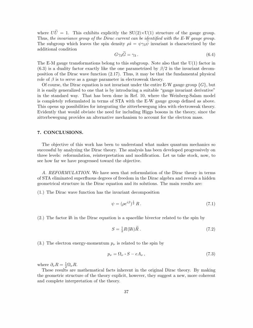
where UU = 1. This exhibits explicitly the SU(2)×U(1) structure of the gauge group.Thus, the invariance group of the Dirac current can be identified with the E-W gauge group.The subgroup which leaves the spin density ρs = ψγ3ψ invariant is characterized by theadditional condition

Gγ3G = γ3 . (6.4)

The E-M gauge transformations belong to this subgroup. Note also that the U(1) factor in(6.3) is a duality factor exactly like the one parametrized by β/2 in the invariant decom-position of the Dirac wave function (2.17). Thus, it may be that the fundamental physicalrole of β is to serve as a gauge parameter in electroweak theory.

Of course, the Dirac equation is not invariant under the entire E-W gauge group G, butit is easily generalized to one that is by introducing a suitable “gauge invariant derivative”in the standard way. That has been done in Ref. 10, where the Weinberg-Salam modelis completely reformulated in terms of STA with the E-W gauge group defined as above.This opens up possibilities for integrating the zitterbewegung idea with electroweak theory.Evidently that would obviate the need for including Higgs bosons in the theory, since thezitterbewegung provides an alternative mechanism to account for the electron mass.

7. CONCLUSIONS.

The objective of this work has been to understand what makes quantum mechanics sosuccessful by analyzing the Dirac theory. The analysis has been developed progressively onthree levels: reformulation, reinterpretation and modification. Let us take stock, now, tosee how far we have progressed toward the objective.

A. REFORMULATION. We have seen that reformulation of the Dirac theory in termsof STA eliminated superfluous degrees of freedom in the Dirac algebra and reveals a hiddengeometrical structure in the Dirac equation and its solutions. The main results are:

(1.) The Dirac wave function has the invariant decomposition

ψ = (ρeiβ)12 R . (7.1)

(2.) The factor ih in the Dirac equation is a spacelike bivector related to the spin by

S = 12R(ih)R . (7.2)

(3.) The electron energy-momentum pν is related to the spin by

pν = Ων · S − eAν , (7.3)

where ∂νR = 12ΩνR.

These results are mathematical facts inherent in the original Dirac theory. By makingthe geometric structure of the theory explicit, however, they suggest a new, more coherentand complete interpretation of the theory.

37

B. REINTERPRETATION. The new zitterbewegung interpretation is imposed on theDirac theory simply by identifying the electron velocity with the lightlike vector u = R(γ0−γ2)R . It follows that the spin S in (7.2) is the angular momentum of the zitterbewegung,and (7.3) attributes energy-momentum to this motion. The general helical character of thezitterbewegung is completely determined by the Dirac equation without further assumption.

This approach has the great formal advantage of providing the entire rotor R with akinematical interpretation. In particular, the complex phase factor is interpreted as adirect representation of the zitterbewegung itself. Thus, a physical explanation is given forthe appearance of complex numbers in quantum mechanics. Moreover, the zitterbewegunginterpretation of the phase factor carries over to Schroedinger theory and so suggests areinterpretation of quantum mechanics generally. This has the great advantage over variantsof the Copenhagen interpretation of being grounded in the Dirac theory.

Above all, the zitterbewegung interpretation presents us with an array of challenges.First, there is a theoretical challenge to see how far we can go in providing zitterbewegunginterpretations for the standard results of quantum mechanics and even quantum electro-dynamics. Second, there is a challenge to probe the zitterbewegung experimentally to seeif it can be established as a “literally real” phenomenon. Finally, there is a challenge to seeif the zitterbewegung can lead us beyond present quantum mechanics to deeper physicalinsights.

C. MODIFICATIONS. If indeed the zitterbewegung is physically real it is probably aconsequence of electromagnetic or electroweak self-interaction, and it may be the source ofan electromagnetic field which fluctuates with the zitterbewegung frequency. Thus it opensup the possibility of a new approach to the self-interaction problem and actually explainingthe phenomenon of quantization rather than assuming it. Of course, such possibilitiescannot be explored theoretically without going beyond the Dirac theory.

REFERENCES

1. D. Hestenes, Space-Time Algebra (Gordon & Breach, London, l966).

2. D. Hestenes, Real Spinor Fields, J. Math. Phys. 8, 798–808 (1967).

4. D. Hestenes, Local Observables in the Dirac Theory, J. Math. Phys. 14, 893–905 (1973).

5. D. Hestenes, Proper Particle Mechanics, J. Math. Phys. 15, 1768–1777 (1974).

6. D. Hestenes, Proper Dynamics of a Rigid Point Particle, J. Math. Phys. 15, 1778–1786(1974).

7. D. Hestenes, Observables, Operators and Complex Numbers in the Dirac Theory, J.Math. Phys. 16, 556-572 (1975).

8. R. Gurtler and D. Hestenes, Consistency in the formulation of the Dirac, Pauli andSchroedinger Theories, J. Math. Phys. 16, 573–583 (1975).

9. D. Hestenes, Spin and Uncertainty in the Interpretation of Quantum Mechanics, Am.J. Phys., 47, 339–415 (1979).

38

10. D. Hestenes, Space-Time Structure of Weak and Electromagnetic Interactions, Found.Phys., 12, l53–l68 (1982).

11. D. Hestenes, Quantum Mechanics from Self-Interaction, Found. Phys. 15, 63–87 (1985).

12. D. Hestenes, Clifford Algebra and the Interpretation of Quantum Mechanics. In Clif-ford Algebras and their Applications in Mathematical Physics, J.S.R. Chisholm& A. K. Common (eds.), (Reidel Publ. Co., Dordrecht/Boston, l986), p. 321–346.

13. D. Hestenes, On Decoupling Probability from Kinematics in Quantum Mechanics. In.Maximum Entropy and Bayesian Methods, Dartmouth College l989, P. Fougere(Ed.) Kluwer, Dordrecht/Boston (1990).

14. D. Hestenes, The Zitterbewegung Interpretation of Quantum Mechanics, Found. Phys.20, 1213–1232 (1990).

15. D. Hestenes and G. Sobczyk, Clifford Algebra to Geometric Calculus, A UnifiedLanguage for Mathematics and Physics, G Reidel Publ. Co., Dordrecht/Boston(1984).

16. D. Hestenes, New Foundations for Classical Mechanics, G. Reidel Publ. Co.,Dordrecht/ Boston (1985).

17. P.A.M. Dirac, Quantum Mechanics, Oxford U. Press, London, 4th edition (1958).

18. D. Hestenes, Vectors, Spinors and Complex Numbers in Classical and Quantum Physics,Am. J. Phys. 39, 1013–1028 (1971).

19. D. Hestenes, A Spinor Approach to Gravitational Motion and Precession, Int. J. Theo.Phys., 25, 589–598 (1986).

20. H.E. Moses, Eigenfunctions of the curl operator, rotationally invariant Helmholtz the-orem, and applications to electromagnetic theory and fluid mechanics. SIAM J. Appl.Math. 21, 114–144 (1971).

21. J. Bjorken and S. Drell, Relativistic Quantum Mechanics, McGraw-Hill, N.Y.(1964).

22. J. Jauch and F. Rohrlich, The Theory of Photons and Electrons, Addison-Wesley,Reading Mass. (1955).

23. J. P. Crawford, On the algebra of Dirac bispinor densities, J. Math. Phys. 26, 1439–1441(1985).

24. T. D. Newton and E. P. Wigner, Localized States for Elementary Systems, Rev. Mod.Phys. 21, 400–406 (1949).

25. R. P. Feynman, Quantum Electrodynamics, Benjamin, N.Y. (1961), p. 47–49.

26. S. Gull, Charged particled in potential steps, In D. Hestenes and A. Weingarthofer(eds.), The ELECTRON, new theory and experiment, Kluwer-Dordrecht/Boston(1991), 37–48 (1991).

27. H. Kruger, private communication.

28. D. Bohm & B. Hiley, Unbroken Quantum Realism, from Microscopic to MacroscopicLevels, Phys. Rev. Letters 55, 2511 (1985).

39

29. C. Philippidis, C. Dewdney and B. J. Hiley, Quantum Interference and the QuantumPotential, Nuovo Cimento 52B, 15–28 (1979).

30. J.-P. Vigier, C. Dewdney, P.R. Holland & A. Kypriandis, Causal particle trajectoriesand the interpretation of quantum mechanics. In Quantum Implications, B. J. Hiley& F. D. Peat (eds.), (Routledge and Kegan Paul, London, 1987).

31. M. P. Silberman, Relativistic time dilatation of bound muons and the Lorentz invarianceof charge, Am. J. Phys. 50, 251–254 (1982).

32. L. S. Brown & T.W.G. Kibble, Interactions of Intense Laser beams with Electrons,Phys. Rev. A 133, 705 (1964).

33. E. Schroedinger, Sitzungb. Preuss. Akad. Wiss. Phys.-Math. Kl. 24, 418 (1930).

34. K. Huang, On the Zitterbewegung of the Electron, Am. J. Phys. 47, 797 (1949).

35. A. O. Barut and A. J. Bracken, Zitterbewegung and the internal geometry of the elec-tron, Phys. Rev. D23, 2454 (1981).

36. T. Uzer, D. Farrelly, J. Milligan, P. Raines & J. Skelton, Celestial Mechanics on aMicroscopic Scale, Science 253, 42–48 (1991).

37. D. Hestenes, Zitterbewegung in Radiative Processes. In D. Hestenes and A. Wein-garthofer (eds.), The ELECTRON, new theory and experiment, Kluwer-Dordrecht/Boston (1991) p. 21–36.

38. D. Hestenes, The Kinematic Origin of Complex Wave Functions. In W.T. Grandy &P.W. Miloni (eds.), Physics and Probability: Essays in Honor of Edwin T.Jaynes, Cambridge U. Press, Cambridge (1993), p. 153–160.

39. D. Hestenes, Zitterbewegung Modeling, Found. Phys. 28, 365–387 (1993).

40. S. Gull, A. Lasenby and C. Doran, Imaginary Numbers Are Not Real—The GeometricAlgebra of Spacetime, Found. Phys. 23, 1175–1202 (1993).

41. P. Lounesto, Clifford Albegras and Hestenes Spinors, Found. Phys. 23, 1203–1238(1993).

42. S. Gull, A. Lasenby and C. Doran, States and Operators in the Spacetime Algebra,Found. Phys. 23, 1239–1264 (1993).

43. H. Kruger, Classical Limit of Real Dirac Theory: Quantization of Relativistic CentralField Orbits, Found. Phys. 23, 1265–1288 (1993).

44. A. Lasenby, C. Doran and S. Gull, A Multivector Derivative Approach to LagrangianField Theory, Found. Phys. 23, 1295–1328 (1993).

45. S. Gull, A. Lasenby and C. Doran, Electron Paths, Tunneling, and Diffraction in theSpacetime Algebra, Found. Phys. 23, 1329–1356 (1993).

46. C. Doran, A. Lasenby, S. Gull, S. Somaroo & A. Challinor, Spacetime Algebra andElectron Physics. In Advances in Imaging and Electron Physics. Academic Press. 95,(1995).

40

APPENDIX A: TRANSFORMATIONS AND INVARIANTS.

This Appendix formulates general transformation laws for fields on spacetime and appliesthe results to establish Poincare invariance of the field equations. The transformation lawfor spinor fields is shown to rest on a convention which can be chosen to make it identicalwith the transformation law for tensor fields.

Let f be a transformation of a 4-dimensional region (or manifold) R = x onto a regionR′ = x′ in a spacetime; the pointwise transformation is thus

f : x→ x′ = f(x) . (A.1)

A transformation is understood to be a differentiable invertible mapping. It induces atransformation f of a vector field a = a(x) on R into a vector field a′ = a′(x′) on R′defined by

f : a→ a′ = fa ≡ a ·5f , (A.2)

where the derivative is evaluated at x = f−1(x′). A parenthesis has been dropped in writingfa in recognition that f is a linear operator on tangent vectors.

The transformation f is called the differential of f . It has a natural extension from vectorfields to arbitrary multivector fields. Thus, for vector fields a1, a2, . . . ak, the differentialof the k-vector field a1 ∧ a2 ∧ · · · ∧ ak is defined by

f(a1 ∧ a2 ∧ · · · ∧ ak) = (fa1) ∧ (fa2) ∧ · · · ∧ (fak) . (A.3)

By linearity this determines the differential for any multivector field M = M(x):

fM =4∑k=0

f(M)(k) , (A.4)

where it is understood that

(fM)(0) = (M)(0) , (A.5)

which is to say that every scalar field is an invariant of f and hence of f . An extensivetreatment of the differential on differentiable manifolds is given in Ref. 15.

The differential of the unit pseudoscalar is given by

fi = idet f , (A.6)

where

det f = i−1 fi = −ifi (A.7)

is the Jacobian of f .As an application of general interest, let us calculate the form of the differential for an

arbitrary infinitesimal transformation

f(x) = x+ ε(x) . (A.8)

41

It is understood that, for any unit vector a, ε · a is a small quantity. This is equivalentto the condition that ε2 is small, except when ε is a null vector. For a vector field thecorresponding induced transformation is

fa = a ·5(x+ ε) = a+ a ·5ε . (A.9)

Neglecting second order terms, therefore, for a bivector field a ∧ b, we have

f(a ∧ b) = a ∧ b+ (a ·5ε) ∧ b+ a ∧ (b ·5ε) = a ∧ b+ [ (a ∧ b) ·5 ] ∧ ε . (A.10)

This result generalizes easily to the differential for an arbitrary multivector field:

fM = M + (M ·5) ∧ ε , (A.11)

where

M ·5 =

4∑k=1

(M)(k) ·5 . (A.12)

Note that k = 0 is not included in the sum since the scalar part of M is invariant.As a significant example, we apply (A.11) to the pseudoscalar i and obtain

fi = i+ (i ·5) ∧ ε = i(1 +5 · ε) . (A.13)

This gives us immediately the useful expression

det f = 1 +5 · ε (A.14)

for the Jacobian of f .Equation (A.11) determines a new function

M ′(x′) = M ′(x+ ε) = M + [M(x) ·5 ] ∧ ε .

To exhibit the ε-dependence of the argument explicitly, we make a Taylor expansion of theargument and keep only first order terms to get

M ′(x) = M(x)− ε ·5M(x) + [M(x) ·5 ] ∧ ε . (A.15)

This tells us explicitly how the infinitesimal transformation changes the field M at a des-ignated point x.

Now let us turn to the question of Poincare invariance of the equations of physics. ThePoincare group is the group of transformations on spacetime which leave invariant the“interval” (x2 − x1)2 between every pair of spacetime points x1 and x2. We are concernedhere only with the Restricted Poincare Group for physical reasons discussed below. Thisis the subgroup of Poincare transformations continuously connected to the identity. Everysuch transformation is the composite of a Lorentz rotation and a translation, so, accordingto (1.24), it can be written in the canonical form

f(x) = RxR + c , (A.16)

42

where c is a constant vector and R is a constant rotor with RR = 1. From (A.2) we findimmediately the differential

a′ = fa = RaR . (A.17)

For the product of two vector fields this gives the simple result

a′b′ = (fa)(fb) = RabR . (A.18)

By virtue of (1.3) this can be decomposed into a scalar part

a′ · b′ = a · b (A.19)

and a bivector parta′ ∧ b′ = f(a ∧ b) = R(a ∧ b)R . (A.20)

According to (A.3), the outer product is an invariant of the differential for any transforma-tion. The inner product and the geometric product are not generally invariant; however,(A.19) and (A.18) show that they are in the present case. It follows that for an arbitrarymultivector field M the transformation law is simply

M ′ = fM = RMR . (A.21)

From this the Poincare invariance of the basic equations of physics is easily established.For example, for Maxwell’s equation (1.28) we have

5′F ′ = (f5)(fF ) = (R5R)(RFR) = R5FR = RJR = J ′ . (A.22)

Thus, the relation of field F to current J is a Poincare invariant.The physical significance of Poincare invariance deserves some comment, since the matter

is frequently muddled in the literature. Poincare transformations are commonly interpretedas relations among different inertial reference systems or observers. That is clearly not thecorrect interpretation here, for no reference system has even been mentioned either inthe formulation of Maxwell’s equation or of its induced transformation (A.22). Indeed,Maxwell’s equation 5F = J is manifestly independent of any coordinate system, so noargument at all is needed to establish its observer independence. The Poincare invarianceexpressed by (A.22) should be interpreted as an equivalence of spacetime points rather thanan equivalence of observers. It describes a physical property of the Minkowski model ofspacetime. Translation invariance implies that spacetime is homogeneous in sense that thesame laws of physics are the same at every spacetime point. Similarly, Lorentz rotationinvariance implies that spacetime is isotropic in the sense that the laws of physics do notfavor any particular timelike or spacelike directions. Poincare invariance thus provides thetheoretical basis for comparing the results of physical experiments and observations madeat different times and places. It is the formal assertion that the laws of physics are thesame everywherewhen.

The Poincare invariance of the Dirac equation (2.5) can be established in the same wayas that of Maxwell’s equation. Thus,

5′ψ′i′h− eAψ′ = (R5R)(RψR)(Ri′R)h− e(RAR)(RψR)

= R(5ψih− eAψ)R = R(mψγ0)R = mψ′γ′0 . (A.23)

43

Note that the transformation law for the spinor wave function ψ has been taken to be

ψ′ = RψR (A.24)

in accordance with (A.21). However, the usual transformation law for a Dirac spinor is

ψ′ = Rψ (A.25)

or, in the conventional matrix representation (2.2),

Ψ′ = RΨ . (A.26)

Nevertheless, the transformation laws (A.24) and (A.25) are physically equivalent, becauseall observables are bilinear functions of the wave function. Indeed, as established by (2.7)

through (2.11), the factor R on the right of (A.24) can be transformed away at will. Thechoice between the transformation laws (A.24) and (A.25) is therefore a matter of conven-tion. Though (A.25) is simpler, (A.24) has the advantage of conformity with (A.21) andhence the more general transformation law (A.4).

In the conventional formulation,21 spinors are defined by the transformation law (A.26),so the possibility of (A.24) does not arise. On the other hand, transformations are notemployed to define spinors in the manifestly invariant STA formulation. Rather, the spinorψ itself represents a transformation as defined by (2.19).

It is of interest to consider briefly the infinitesimal Poincare transformations, since theyplay such a prominent role in the conventional approach to relativistic quantum theory.For an infinitesimal translation, we take R = 1 and ε = c in (A.16), so (A.15) reduces to

M ′(x) = M(x− c) = (1− c ·5)M(x) . (A.27)

This applies equally to the electromagnetic field and the Dirac wave function. Writingc ·5 = cµ∂µ, we recognized the ∂µ as generators of translations. It is noted that the ∂µ canbe made hermitian by the artifice of introducing a unit imaginary factor i′, so the translationoperators in quantum mechanics are usually defined to be i′∂µ. These operators are thenidentified with momentum operators. However, our analysis of the Dirac theory in Section3 reveals that the success of this formal procedure should be attributed to the physicalinterpretation of the Dirac wave function rather than to a general physical significance ofhermitian operators.

For an infinitesimal Lorentz rotation, we take c = 0 in (A.16) and write

R = e12B ≈ 1 + 1

2B , (A.28)

where B is an infinitesimal bivector. Then (A.16) reduces to

x′ = (1 + 12B)x(1− 1

2B) ≈ x+B · x . (A.29)

Hence, ε = B · x in (A.15) and/or (A.30) in (A.21) gives

M ′(x) = [ 1−B · (x ∧5) +B× ]M(x) , (A.30)

44

where B×M is the commutator product. Alternatively, for a spinor ψ subject to the one-sided transformation law (A.27), the result is

ψ′(x) = [ 1−B · (x ∧5) + 12B]ψ(x) . (A.31)

This is expressed in a more conventional form by expanding B with respect to a basis toget

ψ′(x) = (1 + 12B

µνJµν)ψ(x) , (A.32)

where the

Jµν = (γµ ∧ γν) · (x ∧5) + 12γµ ∧ γν = xµ∂ν − xν∂µ + 1

2γµ ∧ γν (A.33)

are the usual “angular momentum operators” for a Dirac particle. In a similar way, angularmomentum operators for the electromagnetic field can be read off (A.30).

APPENDIX B: LAGRANGIAN FORMULATION

This appendix is concerned with the Lagrangian formulation of the Dirac theory. TheLagrange approach has the advantages of ensuring consistency among the various fieldequations and directly relating them to conservation laws. Though this approach to theDirac theory has been discussed many times in the literature, the STA formulation issufficiently novel to merit one more version. A powerful generalization of the presentmethod has since been presented in Ref. 44.

Let L = L(x) be the Lagrangian for some field on spacetime. The associated actionintegral over any region R is

A =

∫RL(x) | d4x | , (B.1)

where the oriented “volume element” for the region is the pseudoscalar

d4x = d1x ∧ d2x ∧ d3x ∧ d4x = i | d4x | . (B.2)

A general variation of the action involves both a change in the functional form of L and aninfinitesimal displacement of R producing a new action

A′ = A+ δA =

∫R′L′(x′) | d4x′ | . (B.3)

For an infinitesimal displacement x→ x′ = x+ ε(x), (A.14) gives us

| d4x′ | = (1 +5 · ε) | d4x | . (B.4)

Hence, writing L′ = L+ δL, to first order we have

δA =

∫R′

(δL+ L5 · ε) | d4x | . (B.5)

45

Now for a given L, both field equations and conservation laws can be derived by requiringthe invariance condition δA = 0 subject to various constraints.

For the Dirac electron, we adopt the (nonunique) Lagrangian

L = 〈 h(5ψ)iγ3ψ − eAψγ0ψ −mψψ 〉 , (B.6)

where 〈 . . . 〉 = (. . .)(0) means “scalar part.” We derive the Dirac equation by requiringδA = 0 for an arbitrary variation δψ(x) = ψ′(x) − ψ(x) in the functional form of thewave function which vanishes on the boundary of R. In this case the boundary is fixedand ε = 0 in (B.5). The derivation employs the scalar-part properties 〈 M 〉 = 〈M 〉 and

〈MN 〉 = 〈NM 〉. Thus, using (δψ)˜ = δψ the variation of the last term in (A.6) can beput in the form

δ〈ψψ 〉 = 〈 (δψ)ψ 〉+ 〈ψδψ 〉 = 2〈ψδψ 〉 .

Similarly, the variation of the second term in (B.6) involves

〈A(δψ)γ0ψ 〉 = 〈ψγ0(δψ)A 〉 = 〈Aψγ0δψ 〉 .

To evaluate the variation of the first term in (B.6), we use δ(5ψ) = 5(δψ) and

〈 (5δψ)iγ3ψ 〉 = 〈5(δψiγ3ψ) 〉 − 〈 δψiγ3(5ψ)˜ 〉= 〈 (5ψ)iγ3δψ 〉+5 · (δψiγ3ψ)(1) . (B.7)

The last term here does not contribute to δA in (B.5), because δψ vanishes on the boundary.Thus, we arrive at

δL = 2〈 (h5ψiγ3 − eAψγ0 −mψ)δψ 〉 . (B.8)

This vanishes for all values of the arbitrary even multivector δψ only if the Dirac equation(2.5) is satisfied.

CONSERVATION LAWS

Conservation Laws are derived by requiring invariance of the action under infinitesimaldisplacements preserving the field equations. For performing the calculation it is convenientto decompose δψ into a part

δ ∗ψ = ψ′(x)− ψ(x) (B.9)

due to a change in the value of ψ and a part due to the shift ε = x′ − x in the argument.This is easily done by writing

δψ = ψ′(x′)− ψ(x) = ψ′(x′)− ψ(x′) + ψ(x′)− ψ(x) .

To first order in small quantities δ ∗ψ(x′) = δ ∗ψ(x) and we have

δψ = δ ∗ψ(x) + ε ·5ψ(x) . (B.10)

46

Applying the same argument to the integrand of (B.5), we have

δL+ L5 · ε = δ ∗L+ ε ·5L+ L5 · ε .

Thus, δA = 0 for any choice of the region R only if

δ ∗L+5 · (εL) = 0 . (B.11)

This is a Conservation Law for specified ε.To evaluate (B.11) for the electron Lagrangian (B.6), we note that δ ∗L will have the

same form as (B.8) except that the perfect divergence term in (B.7) must be included andan additional term due to δ ∗A must be added. However, since we require that the Diracequation be satisfied, the result is simply

δ ∗L = 5 · (hδ ∗ψiγ3ψ)(1) − e〈 δ∗Aψγ0ψ 〉 . (B.12)

Inserting this into (B.11), we can express the general conservation law in the form

5 ·[h(δψ − ε ·5ψ)iγ3ψ + εL

](1)

= e〈 (δA− ε ·5A)ψγ0ψ 〉 . (B.13)

It will be helpful to reformulate this in terms of the energy-momentum operators pµ. Fromthe definition (3.21) we have

ε · pψ = ε ·5ψihγ3γ0 − e ε ·Aψ . (B.14)

So from the definition of the energy-momentum tensor Tµ in (3.24) or Table II, we obtain

ε · Tµ = 〈 γµ(ε · pψ)γ0ψ 〉 . (B.15)

Consequently,

∂µ(ε · Tµ) = ∂µ〈 γµ(ε ·5ψ)ihγ3ψ 〉 − ∂µ(eε ·A〈 γµψγ0ψ 〉) , (B.16)

which relates one term on the left of (B.13) to Tµ. The Lagrangian (B.6) can also beexpressed in terms of Tµ, with the result

L = Tµµ − 〈mψψ 〉 . (B.17)

But we have already observed in (3.31) that this vanishes in consequence of the Diracequation. Finally, we note that the last term in (B.16) can be written

∂µ(ε ·AJµ) = J ·5(ε ·A) , (B.18)

where J = eψγ0ψ is the Dirac charge current. Hence, with the help of the identity

ε · F · J = (ε ·5A) · J − ε · (J ·5A) , (B.19)

47

where F = 5∧A, we can put (B.13) in the form

∂µ(ε · Tµ − 〈 γµδψihγ3ψ 〉) = ε · F · J −A · (J ·5ε)− J · (δA) . (B.20)

This is the desired final form of the general conservation law. Now it is a simple matter toassess the implications of requiring Poincare invariance.

A. Translation Invariance. For an infinitesimal translation ε is constant, δψ = 0, andδA = 0. Hence, (B.20) reduces to

ε · (∂µTµ) = ε · (F · J) . (B.21)

Since ε is arbitrary, this implies the energy-momentum conservation law (3.27). Thus,energy-momentum conservation is a consequence of the homogeneity of spacetime.

B. Lorentz Invariance. For an infinitesimal Lorentz rotation, ε = B · x by (A.29), δA =B×A = B ·A by (A.30), and δψ = (1/2)Bψ by (A.31). In consequence, note the following:

A · [J ·5(B · x) ] = (B · J) ·A = −J · (B ·A) = −J · (δA) ,

ε · Tµ = (B · x) · Tµ = B · (x ∧ Tµ) ,

〈 γµδψiγ3hψ 〉 = 〈Bi(12 hψγ3ψ)γµ 〉 = B · (ρSµ) ,

where Sµ = i(s∧γµ) is the spin angular momentum tensor of (3.33). Inserting these resultsinto (B.20), we obtain

B · [ ∂µ(Tµ ∧ x+ ρSµ) ] = B · [ (F · J) ∧ x ] . (B.22)

SinceB is an arbitrary bivector, this implies the angular momentum conservation law (3.34).Thus, angular momentum conservation is a consequence of the isotropy of spacetime.

For the sake of completeness, we note that a complete Lagrangian for electron and E-Mfields together is obtained by adding to the Dirac Lagrangian (B.6) the term 1

2 〈F 2 〉 =

− 12 〈FF 〉, where F = 5∧A. The electromagnetic part of the Lagrangian is then

LEM = 12 〈F

2 〉 −A · J . (B.23)

The signs have been chosen so that the interaction term agrees with (B.6) for J = eψγ0ψ.From this the E-M field equation can be derived by the general variational principle. Thus,we note that

δ[ 12 〈F

2 〉 ] = 〈F5δA 〉 = δA · (5F ) + ∂µ〈FγµδA 〉 . (B.24)

The last term vanishes for δA = 0 on the boundary, so we have

δLEM = δA · (5F − J) = 0 .

Since δA is arbitrary, this implies Maxwell’s equation 5F = J .

48

Conservation laws for the electromagnetic field can be obtained by inserting (B.23) intothe general Conservation Law (B.11). Thus, using (B.24) with δ∗A = δA − ε ·5A andδ∗J = δJ − ε ·5J , we obtain

∂µ[〈Fγµε ·5A 〉 − 1

2γµ · ε〈F 2 〉 − 〈FγµδA 〉

]= −J · (ε ·5A)−A · (δJ)− (J ·A)5 · ε . (B.25)

Let us define the canonical energy-momentum tensor Tµc = Tc(γµ) by

Tc(n) ≡ −12FnF − n · F · 5A

= 5〈FnA 〉 − 12n〈F

2 〉+A〈n5F 〉 , (B.26)

where the reverse accents serve to indicate which functions are differentiated by5. Insertingthis into (B.25), we get the Conservation Law in the form

∂µ[ ε · Tµc − 〈FγµδA 〉 ] = ε · (J · F ) +A · (J ·5ε)−A · (δJ)− J ·A5 · ε . (B.27)

As before, translation invariance yields the energy-momentum conservation law

∂µTµc = J · F = −F · J . (B.28)

And Lorentz invariance yields the angular momentum conservation law

∂µ[Tµc ∧ x+ Sµc ] = (J · F ) ∧ x , (B.29)

where the E-M spin tensor Sµc = Sc(γµ) is given by

Sc(n) = (F · n) ∧A . (B.30)

Of course, both (B.28) and (B.29) can be obtained by direct differentiation of (B.26). Alsonote that when they are added to the corresponding equations (3.27) and (3.34) for theelectron, the internal forces and torques cancel.

49