Embed Size (px)
DESCRIPTION
Mfix Manual
Citation preview

Release 2013-2 September 2013

MFIX 2013-2 Readme file
Page 2 of 113
Image credits:
Cover page: Aaron Morris, University of Colorado at Boulder: MFIX-DEM simulation of solids falling through an array of hexagonal tubes.
Page 7, top: Aytekin Gel, ALPEMI Consulting, LLC: MFIX-TFM simulation of coal jet penetration, colored by CO2 species mass fraction.
Page 7, bottom: Jordan Musser, DOE NETL: Reactive MFIX-DEM simulation of a spouted bed, particles colored by temperature.
Page 8, top: Rahul Garg, URS E&C Inc.: MFIX-PIC simulation of a cyclone, showing particles and streamlines, colored by velocity.
Page 8, bottom: Jordan Musser, DOE NETL: MFIX-Hybrid simulation of a bubbling bed with two solids phases (one continuous phase and one discrete phase). The background is colored by solids bulk density (continuous phase) and spheres represent the second solids phase.

MFIX 2013-2 Readme file
Page 3 of 113
Notice
Neither the United States Government nor any agency thereof, nor any of their employees, makes any warranty, express or implied, or assumes any legal liability or responsibility for the accuracy, completeness, or usefulness of any information, apparatus, product, or process disclosed or represents that its use would not infringe privately owned rights.
• MFIX is provided without any user support for applications in the user's immediate organization. It should not be redistributed in whole or in part.
• The use of MFIX is to be acknowledged in any published paper based on computations using this software by citing the MFIX theory manual. Some of the submodels are being developed by researchers outside of NETL. The use of such submodels is to be acknowledged by citing the appropriate papers of the developers of the submodels.
• The authors would appreciate receiving any reports of bugs or other difficulties with the software, enhancements to the software, and accounts of practical applications of this software.
Disclaimer
This report was prepared as an account of work sponsored by an agency of the United States Government. Neither the United States Government nor any agency thereof, nor any of their employees, makes any warranty, express or implied, or assumes any legal liability or responsibility for the accuracy, completeness, or usefulness of any information, apparatus, product, or process disclosed, or represents that its use would not infringe privately owned rights. Reference herein to any specific commercial product, process, or service by trade name, trademark, manufacturer, or otherwise does not necessarily constitute or imply its endorsement, recommendation, or favoring by the United States Government or any agency thereof. The views and opinions of authors expressed herein do not necessarily state or reflect those of the United States Government or any agency thereof.
MFIX 2013-2 Readme file
Page 4 of 113
Table of Contents
1. Introduction ........................................................................................................... 6
2. Development state of MFIX models ........................................................................ 7
3. 2013-2 Release notes ............................................................................................ 9
4. Setting Up and Running MFIX on a UNIX/LINUX Workstation ............................... 10
4.1. Creating MFIX Directory ....................................................................................... 10
4.2. Alias creation ....................................................................................................... 11
4.3. Creation of executable files .................................................................................. 12
4.3.1. MFIX Makefiles ............................................................................................. 13
4.3.2. Compiling MFIX for the first time: A step-by-step example .............................. 15
4.3.3. Compiling POSTMFIX ................................................................................... 17
4.4. Visualizing Data with ParaView ............................................................................ 19
4.5. Starting a New Run .............................................................................................. 20
4.6. Modifying the Post-Processing Codes .................................................................. 24
5. Setting Up and Running MFIX on Windows Workstation ....................................... 24
5.1. Installing MFIX on Windows OS ........................................................................... 24
5.2. Installing the MFIX Code using Cygwin on Windows OS ....................................... 24
6. MFIX at Run Time ................................................................................................ 26
6.1. MFIX Output and Messages ................................................................................. 26
6.2. Restarting a Run .................................................................................................. 28
6.3. When the Run Does Not Converge ...................................................................... 28
7. Keywords in Input Data File (mfix.dat) .................................................................. 29
7.1. Run Control ......................................................................................................... 30
7.2. Physical Parameters ............................................................................................ 36
7.3. Numerical Parameters ......................................................................................... 39
7.4. Geometry and Discretization ................................................................................ 44
7.5. Gas Phase .......................................................................................................... 47
7.6. Solids Phase ....................................................................................................... 47
7.7. Initial Conditions .................................................................................................. 48
7.8. Boundary Conditions ........................................................................................... 51
7.9. Internal Surfaces ................................................................................................. 59
7.10. Point Source Mass Inlets ............................................................................... 61
MFIX 2013-2 Readme file
Page 5 of 113
7.11. Output Control ............................................................................................... 63
7.12. Chemical Reactions – basic options ............................................................... 65
7.13. Chemical reactions – advanced options .......................................................... 80
7.14. Thermochemical Properties ........................................................................... 82
7.15. User-Defined Subroutines ............................................................................. 84
7.16. Parallelization Controls .................................................................................. 87
7.17. MFIX Execution in Batch Queue Environment ................................................ 88
7.18. Discrete Element Model (DEM) ...................................................................... 90
7.19. MPPIC model: ............................................................................................. 103
7.20. Direct Quadrature Method of Moments (DQMOM) ........................................ 106
7.21. Quadrature Method of Moments (QMOM) .................................................... 107
7.22. Cohesion Model in DEM .............................................................................. 107
7.23. Cartesian grid .............................................................................................. 111
8. Mailing lists ........................................................................................................ 112
9. User contribution ............................................................................................... 113
MFIX 2013-2 Readme file
Page 6 of 113
1. Introduction
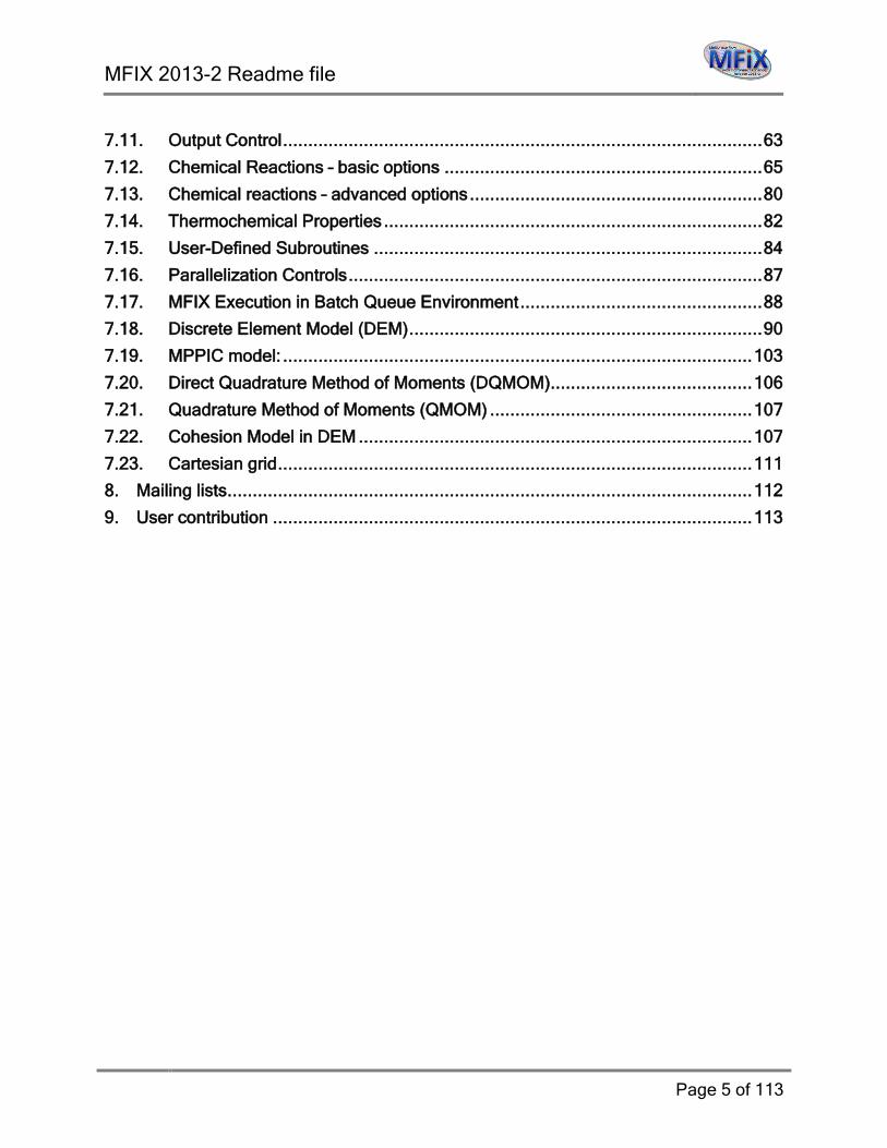
MFIX is an open-source multiphase flow solver and is therefore free to download and use. A one-time free registration is required prior to downloading the source code. To register, go to the MFIX website at https://mfix.netl.doe.gov, click on "Register" at the bottom of the home page or go directly to https://mfix.netl.doe.gov/registration.php. Complete the form, read the notice and click on "I Agree" to submit your application. Once your application has been reviewed and accepted, you will receive an email notification, and instructions to download the code.
The above flow chart provides an overview of the work flow and related sections in this document for quick review.
Some Frequently Asked Questions located at https://mfix.netl.doe.gov/faq.php may be useful to review before downloading MFIX.
MFIX Installation
(Sections 4.1 to 4.3)
MFIX Input setup (Sections 7)
Run MFIX
(Sections 4.5 & 6)
Post-processing & Visualization
(Sections 4.3.3 & 4.4)

MFIX 2013-2 Readme file
Page 7 of 113
2. Development state of MFIX models
MFIX provides a suite of models that treat the carrier phase (typically the gas phase1) and disperse phase (typically the solids phase) differently. Their current state of development is summarized in the tables below.
• Two Fluid Model: MFIX-TFM (Eulerian-Eulerian)
Both gas and solids phases are treated as interpenetrating continuum phases.
Serial †DMP ‡SMP
Continuity Equations ● ● ●
Momentum Equations ● ● ●
Energy Equations ● ● ●
Species Equations ● ● ●
Chemical Reactions ● ●
Cartesian cut-cell ● ● □
• Discrete Element Method: MFIX-DEM (Eulerian-Lagrangian)
The gas phase is treated as continuum and particles positions are tracked individually. Particle collisions are directly resolved.
Serial †DMP ‡SMP Momentum Equations ● ● ● Energy Equations ● Species Equations ● Chemical Reactions ● Cartesian cut-cell ○ □
1 For bubbly gas-liquid flows, the carrier phase would be the liquid phase and the disperse phase would be the gas bubbles.
MFIX 2013-2 Readme file
Page 8 of 113
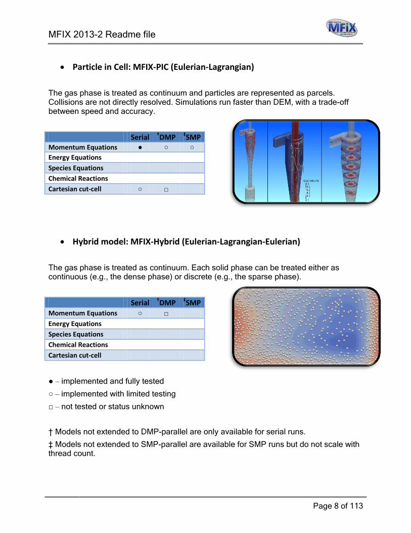
• Particle in Cell: MFIX-PIC (Eulerian-Lagrangian)
The gas phase is treated as continuum and particles are represented as parcels. Collisions are not directly resolved. Simulations run faster than DEM, with a trade-off between speed and accuracy.
Serial †DMP ‡SMP Momentum Equations ● ○ ○ Energy Equations Species Equations Chemical Reactions Cartesian cut-cell ○ □
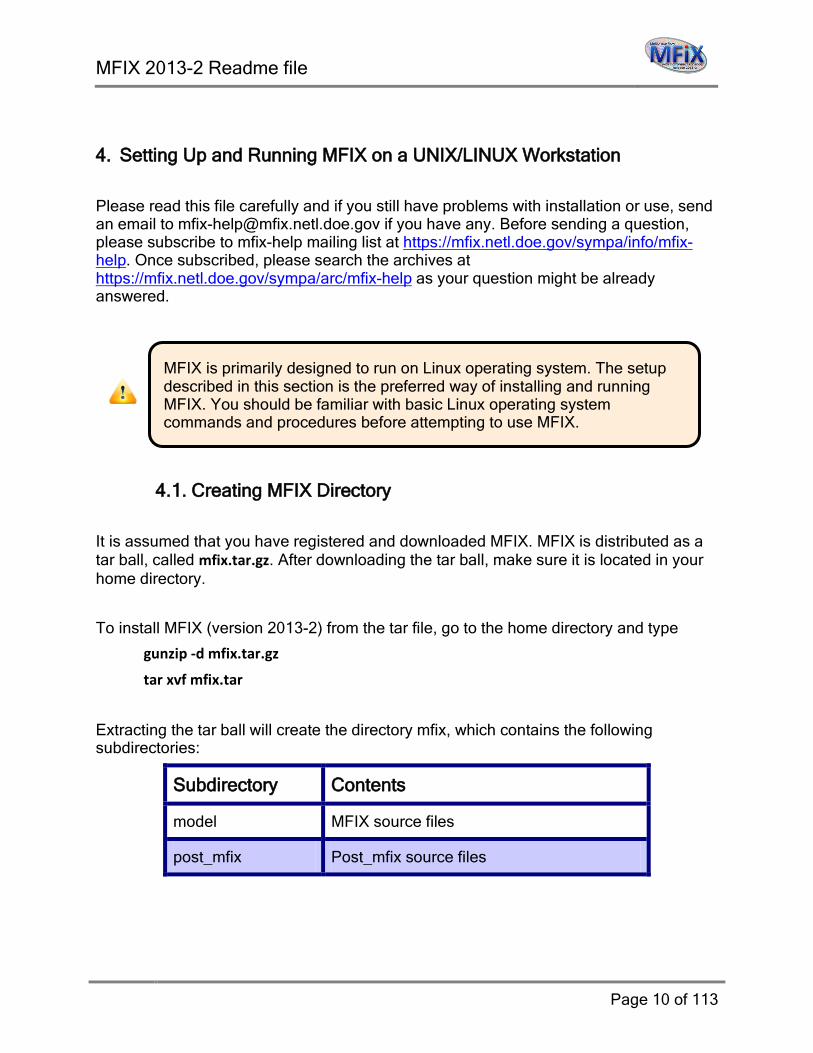
• Hybrid model: MFIX-Hybrid (Eulerian-Lagrangian-Eulerian)
The gas phase is treated as continuum. Each solid phase can be treated either as continuous (e.g., the dense phase) or discrete (e.g., the sparse phase).
Serial †DMP ‡SMP Momentum Equations ○ □ Energy Equations Species Equations Chemical Reactions Cartesian cut-cell
● – implemented and fully tested ○ – implemented with limited testing
□ – not tested or status unknown
† Models not extended to DMP-parallel are only available for serial runs.
‡ Models not extended to SMP-parallel are available for SMP runs but do not scale with thread count.

MFIX 2013-2 Readme file
Page 9 of 113
3. 2013-2 Release notes
For MFIX users upgrading to the 2013-2 Release, please note the following changes from the previous (2013-1) release:
New features added:
• Stiff chemistry solver The stiff chemistry solver was completely overhauled to eliminate any user-coding. This capability can now be activated with a single keyword (section 7.13).
• Point source The ability to specify mass inlet point source anywhere in the domain was added. This can be useful when modeling a small side inlet, without having to resolve the actual geometry (section 7.10).
• Subgrid models The two-fluid Igci and Milioli filtered models were implemented and can be activated by new keywords (page 35).
• DEM cluster detection An algorithm to detect clusters and collect information was implemented (page 102).
Changes in existing features:
• Parallel execution The SMP directives have been updated in key-subroutines. The SMP compilation options (including hybrid SMP+DMP) have been turned back on. Please note that the reported CPU time may be inaccurate in SMP mode.
MFIX 2013-2 Readme file
Page 10 of 113
4. Setting Up and Running MFIX on a UNIX/LINUX Workstation
Please read this file carefully and if you still have problems with installation or use, send an email to [email protected] if you have any. Before sending a question, please subscribe to mfix-help mailing list at https://mfix.netl.doe.gov/sympa/info/mfix-help. Once subscribed, please search the archives at https://mfix.netl.doe.gov/sympa/arc/mfix-help as your question might be already answered.
4.1. Creating MFIX Directory
It is assumed that you have registered and downloaded MFIX. MFIX is distributed as a tar ball, called mfix.tar.gz. After downloading the tar ball, make sure it is located in your home directory.
To install MFIX (version 2013-2) from the tar file, go to the home directory and type
gunzip -d mfix.tar.gz
tar xvf mfix.tar
Extracting the tar ball will create the directory mfix, which contains the following subdirectories:
Subdirectory Contents
model MFIX source files
post_mfix Post_mfix source files
MFIX is primarily designed to run on Linux operating system. The setup described in this section is the preferred way of installing and running MFIX. You should be familiar with basic Linux operating system commands and procedures before attempting to use MFIX.
MFIX 2013-2 Readme file
Page 11 of 113
tutorials Several example problems and corresponding pdf files describing some of the tutorials exists, which are useful for a new user
tests Test simulations used to verify the code during development
visualization_tools Tools to visualize MFIX results (not supported anymore)
tools Development tools
doc MFIX manuals in pdf format
4.2. Alias creation
For convenience, create aliases by adding the following lines to the .login or the .cshrc file (assuming MFIX was installed in the home directory, and you are using the C shell):
alias mkmfix sh ~/mfix/model/make_mfix
alias post ~/mfix/post_mfix/post_mfix
After adding the aliases in the .login or .cshrc file, the user should logout and login or type: source .login so that the aliases are functional. This step needs to be done only once. Then the mfix make file can be invoked from any directory by typing mkmfix, and the post-processor can be activated by typing post. The creation and utilization of aliases is not required to use MFIX. Aliases provide convenient shortcuts to common commands.
Note that makefile should be invoked as “sh make_mfix.” Erroneously invoking it as “make_mfix” will cause the user-defined files not to be used for the build. The alias for post_mfix will be operational when post_mfix is compiled (see section 2.3.2).
MFIX 2013-2 Readme file
Page 12 of 113
4.3. Creation of executable files
Installing MFIX only requires to convert the source code into an executable file. This is called the compilation of the code. You need a Fortran compiler to compile MFIX. Before continuing, make sure you have a working Fortran compiler on your computer. Please contact your system administrator if you are not sure how to properly install and test the compiler.
The distribution of MFIX provides two sets of source codes:
Name Purpose Location of source code
Name of executable
MFIX Multiphase flow solver ~/mfix/model mfix.exe
POSTMFIX Simple post processing of the data. This is a text-based program. Data is extracted based on (I,J,K) location in the computational domain.
~/mfix/post_mfix post_mfix
The open-source visualization tools ParaView and VisIt can be used to visualize and post-process MFIX results. They can be downloaded from:
ParaView: http://www.paraview.org/
VisIt: https://wci.llnl.gov/codes/visit/home.html
Please follow the instructions on the above websites to install ParaView or VisIt.
MFIX 2013-2 Readme file
Page 13 of 113
4.3.1. MFIX Makefiles
Both MFIX and POSTMFIX are compiled through a makefile, called make_mfix for MFIX and make_post for POSTMFIX. It is not expected that these files need to be modified, but expert users may edit the makefiles to add compilations options or flag specific to their architecture. The next section focuses on make_mfix, due to the availability of several flags. Invoking make_post is best described by following the example in section 2.3.3.
Basic usage
Invoke make_mfix without arguments to go through the list of options. This is the standard input method where the user manually answers questions to compile MFIX. To invoke the makefile, type
sh ~/mfix/model/make_mfix
or
mkmfix
if you created the alias (section 2.2). The following examples assume the alias is created.
Compiling with default options
Use the -default flag to compile with the default options:
- Serial,optimized code
- Re-compilation of source files is not forced
- GNU Fortran compiler
mkmfix -default
Repeating a compilation
Use the -repeat flag to recompile with the same options as the last successful compilation.
mkmfix –repeat
Showing all compiler options
Some compilers available on very specific systems are hidden by default. Use the -long
MFIX 2013-2 Readme file
Page 14 of 113
flag to display all compiler options.
mkmfix -long
Cleaning-up a previous compilation
Use the -clean flag before doing a fresh compilation. This option will remove all .o, .a and .mod files from the object directory (last compilation). The makefile must be invoked again if a new compilation is needed.
mkmfix -clean
mkmfix
Showing a help message
Use the -help flag to display a help message that summarizes available options.
mkmfix -help
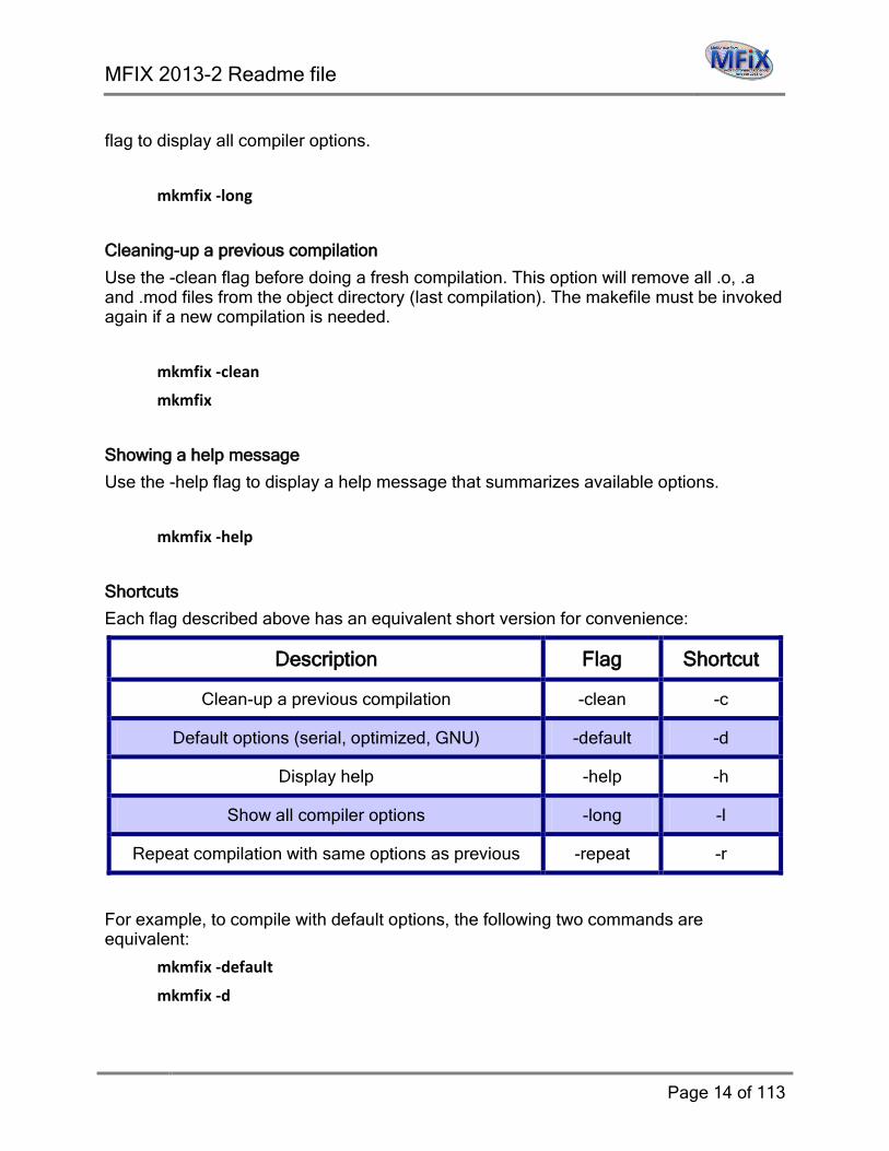
Shortcuts
Each flag described above has an equivalent short version for convenience:
Description Flag Shortcut
Clean-up a previous compilation -clean -c
Default options (serial, optimized, GNU) -default -d
Display help -help -h
Show all compiler options -long -l
Repeat compilation with same options as previous -repeat -r
For example, to compile with default options, the following two commands are equivalent:
mkmfix -default
mkmfix -d
MFIX 2013-2 Readme file
Page 15 of 113
4.3.2. Compiling MFIX for the first time: A step-by-step example
Before compiling MFIX, you must be sure to have a working Fortran compiler installed on your computer (i.e., can compile a simple Fortran code such as print hello and link to create an executable). In the following example, it is assumed that the gfortran compiler is installed on a 64-bit computer. MFIX will be compiled and run for a simple fluidbed tutorial case. At this point, it is not important to understand the simulation setup. The executable file mfix.exe will be created for serial execution.
1) Go to the tutorial directory:
cd ~/mfix/tutorial/fluidbed1
2) This folder contains the input file mfix.dat that contains the simulation setup. This file is not required to compile MFIX, but will be used at the end of this example to run the simulation. MFIX can be compiled from any directory, except the /mfix/model directory. The directory where MFIX will be run is called the run directory. Here the run directory is fluidbed1, and currently only contains the mfix.dat file. Display the content of the directory:
ls
3) Compile MFIX
3a) Invoke the makefile.
mkmfix
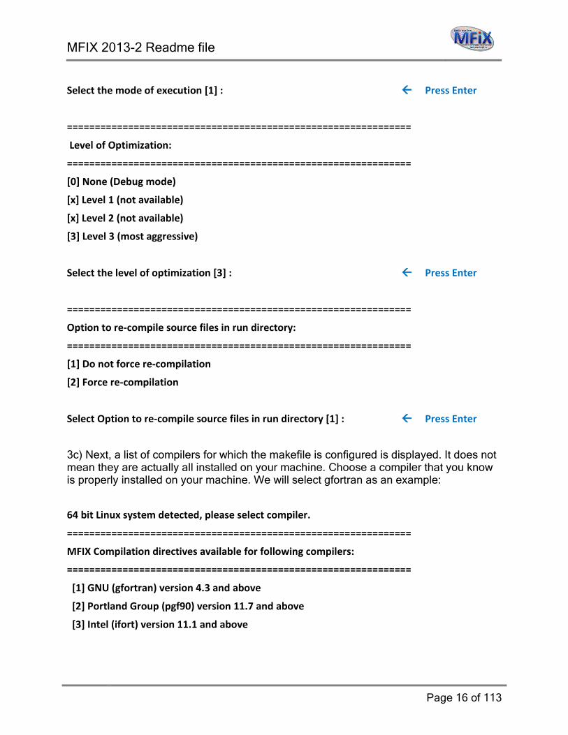
3b) You will be prompted to answer 3 questions. Press Enter to keep the default answers to all 3 questions. This will compile MFIX in optimized serial mode.
==============================================================
Mode of execution:
==============================================================
[1] Serial
[2] Parallel, Shared Memory (SMP)
[3] Parallel, Distributed Memory (DMP)
[4] Parallel, Hybrid (SMP+DMP)
MFIX 2013-2 Readme file
Page 16 of 113
Select the mode of execution [1] : Press Enter
==============================================================
Level of Optimization:
==============================================================
[0] None (Debug mode)
[x] Level 1 (not available)
[x] Level 2 (not available)
[3] Level 3 (most aggressive)
Select the level of optimization [3] : Press Enter
==============================================================
Option to re-compile source files in run directory:
==============================================================
[1] Do not force re-compilation
[2] Force re-compilation
Select Option to re-compile source files in run directory [1] : Press Enter
3c) Next, a list of compilers for which the makefile is configured is displayed. It does not mean they are actually all installed on your machine. Choose a compiler that you know is properly installed on your machine. We will select gfortran as an example:
64 bit Linux system detected, please select compiler.
==============================================================
MFIX Compilation directives available for following compilers:
==============================================================
[1] GNU (gfortran) version 4.3 and above
[2] Portland Group (pgf90) version 11.7 and above
[3] Intel (ifort) version 11.1 and above

MFIX 2013-2 Readme file
Page 17 of 113
Select the compiler to compile MFIX? [1] Press Enter
3d) The compilation should start and may take several minutes to complete. Once the compilation is successful, the executable file mfix.exe is created and ready to use.
*******************************************
Compilation successful: mfix.2013-2 created
To run MFIX type: mfix.exe
*******************************************
4) Run MFIX:
./mfix.exe
As the solution proceeds, a lot of information is displayed on the screen. Please see section 4 for a description of the output. The run should complete in a few minutes.
4.3.3. Compiling POSTMFIX
You can use POSTMFIX to extract data at a particular location in the flow field. To compile POSTMFIX, follow the following procedure. Again, it is assumed that gfortran is installed.
1) Go to the post_mfix folder:
cd ~/mfix/post_mfix
2) Invoke the make file:
sh make_post
3) A list of compilers will be displayed, based on your operating system. Again, this list means the makefile is configured to use those compilers, but does not imply they are installed on your computer. In our case, we will select the gfortran compiler. Answering no (n) to the first three questions will select gfortran.
MFIX 2013-2 Readme file
Page 18 of 113
Linux system with 64 bit processor detected, please select compiler
MFIX Compilation directives available for following compilers:
- Intel Fortran Compiler (IFORT - FCE for 64 bit)
- Portland Group Linux Fortran Compiler (pgf90)
- PathScale compiler (pathf90)
- gfortran
Do you want to compile with Intel Compiler? (y/n) [yes] n Type n and press Enter
Do you want to compile with Portland Group Compiler? (y/n) [yes] n Type n and press Enter
Do you want to compile with PathScale Compiler? (y/n) [yes] n Type n and press Enter
gfortran selected
4) Before continuing, delete object files:
Object files (*.o, *.mod, *.a) in mfix/model will be deleted. Continue? (y/n) [no] y Type y and press Enter
5) The compilation will start, and upon successful compilation, the following message will be displayed:
********************************************
* Compilation successful: post_mfix created*
********************************************
Once post_mfix is successfully compiled, the alias created in Section 2.2 is operational.
MFIX 2013-2 Readme file
Page 19 of 113
4.4. Visualizing Data with ParaView
It is assumed you have downloaded and installed a suitable binary version of ParaView. To visualize MFIX results, Launch ParaView, and go to File > Open, (or click on the icon) and select the .RES file in the run directory. For example, to visualize the results from the fluidbed1 tutorial, open the BUB01.RES file. Next, click on the green “Apply” button on the left pane to load all variables. This step may be optional on your version of ParaView. You will see a contour plot of the void fraction (EP_g). To show an animation of void fraction, press the play button in the animation toolbar . You will see bubbles forming along the left boundary and moving upward. This tutorial is using a 2D cylindrical coordinate system, and the left boundary is the axis of symmetry of the system. Only one side was simulated due to symmetry. To visualize the entire system, go to Filter >Alphabetical>Reflect. In the Object inspector, select Plane X, and Center 0, and click Apply. You should see the complete symmetric system now, with bubbles forming in the center.
MFIX 2013-2 Readme file
Page 20 of 113
4.5. Starting a New Run
If you have successfully completed your first compilation of MFIX as described in Section 2.3.1, you are ready to explore other options to compile and run MFIX, with your own simulation setup.
Create a separate subdirectory for each run, referred to as the run directory.
Create an MFIX executable file by typing mkmfix. The MFIX executable file mfix.exe will be created and copied into the run-directory.
First, select the type of executable (currently, only serial and DMP options are available). Regardless of the option chosen here, the executable is always named mfix.exe
==============================================================
Mode of execution:
==============================================================
[1] Serial
[2] Parallel, Shared Memory (SMP)
[3] Parallel, Distributed Memory (DMP)
[4] Parallel, Hybrid (SMP+DMP)
Select the mode of execution [1] :
Type 1 for serial code or 3 for DMP code and press Enter.
Note: To keep the default answer (1 = serial), just press Enter.
If you want to modify MFIX subroutines, do the following. Copy the subroutine from the mfix/model directory into the run directory. Modify the file copied to the run directory. Do not modify the files in the mfix/model directory.
MFIX 2013-2 Readme file
Page 21 of 113
Next, select the level of optimization:
==============================================================
Level of Optimization:
==============================================================
[0] None (Debug mode)
[x] Level 1 (not available)
[x] Level 2 (not available)
[3] Level 3 (most aggressive)
Select the level of optimization [3] :
Type 0 and press Enter for executable in debug mode. This option is useful if you modified some source files and want to test the code for possible bugs before production run. Execution time will be much slower in debug mode than in optimized mode.
Press Enter to keep the default answer (3). This will generate an optimized executable, which will run faster for production run.
==============================================================
Option to re-compile source files in run directory:
==============================================================
[1] Do not force re-compilation
[2] Force re-compilation
Select Option to re-compile source files in run directory [1] :
If you intend to compile the DMP version of MFIX, please verify that your MPI installation works properly (see MPI_verification_for_MFIX.pdf document in /mfix/tools/mpi). Contact your system administrator if you are not sure how to proceed.

MFIX 2013-2 Readme file
Page 22 of 113
Type 2 and press Enter to make sure source files in the run directory are compiled. This option is needed only in the rare instances when the run directory contains a module file (e.g., run_mod.f) and another file (e.g., usr0.f), in which the corresponding use statement has been inserted (e.g., use run). The makefile will not be aware of this dependency (usr0 depends upon run). So, in this example, changes made in run_mod.f will not cause the (necessary) recompilation of usr0.f, unless this option is selected.
Press Enter to keep the default answer (1).
If you keep all the above default options by pressing Enter for each question, an optimized serial version executable will be produced for that particular platform.
Finally, a list of compilers is proposed for your system:
==============================================================
MFIX Compilation directives available for following compilers:
==============================================================
[1] GNU (gfortran) version 4.3 and above
[2] Portland Group (pgf90) version 11.7 and above
[3] Intel (ifort) version 11.1 and above
Select the compiler to compile MFIX? [1]
Type the number corresponding to the compiler you want to use, and press Enter. If you want to use the default option (1 = GNU gfortran), just press Enter.
After selecting the compiler, the compilation process will start. At the end of the compilation process, you should have the executable mfix.exe in this directory.
If you have compiled MFIX once, you can run make_mfix with the same options by invoking the makefile with the flag –repeat or –r. For example
mkmfix –r
will repeat the compilation process with the last known configuration. This is useful if you compile MFIX many times during your own development phase, and do not wish to keep entering the same input over and over.
MFIX 2013-2 Readme file
Page 23 of 113
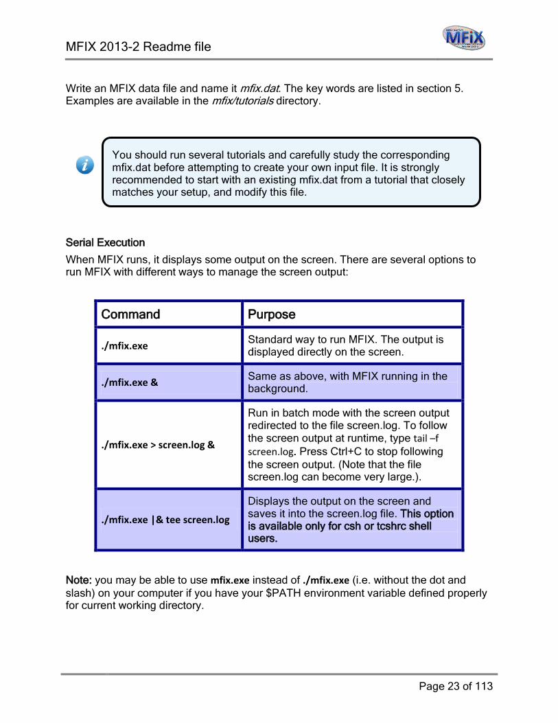
Write an MFIX data file and name it mfix.dat. The key words are listed in section 5. Examples are available in the mfix/tutorials directory.
Serial Execution
When MFIX runs, it displays some output on the screen. There are several options to run MFIX with different ways to manage the screen output:
Command Purpose
./mfix.exe Standard way to run MFIX. The output is displayed directly on the screen.
./mfix.exe & Same as above, with MFIX running in the background.
./mfix.exe > screen.log &
Run in batch mode with the screen output redirected to the file screen.log. To follow the screen output at runtime, type tail –f screen.log. Press Ctrl+C to stop following the screen output. (Note that the file screen.log can become very large.).
./mfix.exe |& tee screen.log
Displays the output on the screen and saves it into the screen.log file. This option is available only for csh or tcshrc shell users.
Note: you may be able to use mfix.exe instead of ./mfix.exe (i.e. without the dot and slash) on your computer if you have your $PATH environment variable defined properly for current working directory.
You should run several tutorials and carefully study the corresponding mfix.dat before attempting to create your own input file. It is strongly recommended to start with an existing mfix.dat from a tutorial that closely matches your setup, and modify this file.

MFIX 2013-2 Readme file
Page 24 of 113
Parallel Execution
Run the DMP version using mpirun -np <Number of Processors> mfix.exe . This command may be different on other machines (e.g., mpprun -n <Number of Processors> mfix.exe). Recent versions of MPI library (i.e., MPICH2 on Linux clusters) require mpi daemons running on the compute nodes prior to the launch of any mpi executable. Please make sure the appropriate MPI initialization procedures are followed and the simple MPI examples run successfully to verify MPI setup prior to the launch of MFIX executable in DMP mode.
Note that MFIX results can be retrieved, even while the run is in progress.
To retrieve and manipulate data and to create special restart files, run the post_processor post_mfix by typing post. post_mfix will prompt the user for the run name. Enter the run name (e.g., BUB01 ).
4.6. Modifying the Post-Processing Codes To make post_mfix, first change the directory to the mfix/post_mfix directory. If user-defined post-processing is required, modify the usr_post.f file in the directory. Then type sh make_post. Note that the mfix/model is required for creating a post_mfix executable.
5. Setting Up and Running MFIX on Windows Workstation
5.1. Installing MFIX on Windows OS This is not very well supported; please see our download page (https://mfix.netl.doe.gov/members/download.php) for special remarks (https://mfix.netl.doe.gov/members/wininst.html) and also earlier postings on mfix-help mailing list.
5.2. Installing the MFIX Code using Cygwin on Windows OS
1. Install Cygwin from http://www.cygwin.com/ . To get more familiar with Linux/Unix - you can do a google search on unix primer (http://www.google.com/search?q=unix++primer) or you can see the top hit (http://bignosebird.com/unix.shtml)
2. Check that Devel and Editors are installed (To the right of the words will be "default"; Left button click on the word "default" until it says "install")
3. Make sure that make and ex are installed

MFIX 2013-2 Readme file
Page 25 of 113
$ which ex /usr/bin/ex $ which make /usr/bin/make
4. Now install gfortran (this is now part of gcc)
Check that gfortran is available (by typing gfortran on console, you should get 'gfortran: no input files')
5. Download MFIX from our website, and go to the directory where the MFIX tar ball was saved.
6. issue this command "tar -xzvf mfix.tar.gz" 7. go to tutorials/fluidbed1 by typing "cd mfix/tutorials/fluidbed1" 8. Issue the command "sh ../../model/make_mfix"
This should start the compilation process and depending on the computer this might take a long time.
At the end you should have the executable mfix.exe in this directory. To list the files you can use the 'ls' command
9. Now issue the command "nohup ./mfix.exe > out1&" - this will launch the program in the background.
10. You can see the output from the out file by issuing command "tail -f out1". This would stop as soon as the program finished executing.
11. You can visualize the output using ParaView (http://www.paraview.org). 12. Any questions check the archives of mfix-help and if you are still having a problem,
email [email protected] by providing the following important details in your message after the description of the problem encountered:
1. MFIX version you are trying to install or run 2. Some details on your operating system environment (for Linux: copy and
paste the response of uname –a command, Linux distribution name and version also)
3. Your compiler name and version number (e.g. ifort –v will give the version number for Intel fortran compiler)
4. Output for your $PATH environment (in csh type echo $PATH) 5. Your MPI library name and version number (if compilations problem with
DMP mode encountered but make sure you can compile and run a simple hello world type MPI program with your current installation) Also please provide hardware details such as number of cores per socket in your system (or send the output for “cat /proc/cpuinfo“ and how many cores you are trying to utilize.

MFIX 2013-2 Readme file
Page 26 of 113
6. MFIX at Run Time
6.1. MFIX Output and Messages MFIX output is stored in nine *.SPx binary files. The restart info is periodically written to the *.RES binary file. The text file *.OUT echos the input, shows the numerical cell distribution, and, if OUT_DT is defined, prints the field variables at the specified intervals.
The text file *.LOG contains run information. For the DMP version, a LOG file is created for each of the processors and they are numbered as Name###.LOG.
Messages about the run are written to the .LOG file. The progress of the run will be displayed at the terminal as shown below if the data file specifies FULL_LOG = .TRUE.
The first line shows the time, the time-step, and the CPU time remaining to complete the run. The CPU time remaining is not accurate, especially in the beginning of the run. For each time-step, the normalized residuals for various equations are written out every iteration.
MFIX uses a variable time step, which is automatically adjusted within user-defined limits to reduce the run time. At large values of Dt, the iterations may not converge. When this happens, the time step size is successively reduced until convergence is obtained. Messages about divergence and recovery are displayed on the terminal and in the .LOG file, if FULL_LOG = .TRUE.
The subsequent lines display the iteration number, the normalized residuals for various equations (e.g., gas continuity, solids continuity, x and y gas momentum, and x and y solids momentum), and the equation with the maximum residual. The residuals P0 and P1 are normalized only when Nit>1. The residuals displayed can be selected with the keyword RESID_STRING.

MFIX 2013-2 Readme file
Page 27 of 113
MFIX reports errors while reading the data file, while processing input data, and during the run time. Errors in reading the data file and in opening files are reported to the terminal. All other errors are reported in the .LOG file.
While reporting errors in reading the data file, MFIX displays the offending line of input, so that the error can be easily detected. The possible causes of error are (1) incorrect format for the name-list input, (2) unknown (misspelt) variable name, or (3) the dimension of the name-list item is too small. For example, if the dimension of DX is set as 5000 (DIM_I in param_mod.f ), and if the input data file contains an entry DX(5001), MFIX will report an input processing error.
While processing the input data, MFIX will report errors if the data specified is insufficient or physically unrealistic. MFIX will supply default values only when it is certain that giving a default value is reasonable.
An occasional input-processing error is the inability to determine the flow plane for a boundary condition. The boundary planes defined in the input data file must have a wall-cell on one side and a fluid-cell on the other side. If the initial condition is not specified for the fluid-cell, MFIX will not recognize the cell as a fluid-cell and, hence, MFIX will be unable to determine the flow plane.
Every NLOG number of time steps, MFIX monitors whether the mass fractions add up to 1.0; the overall reaction rates add up to zero; the viscosities, conductivities, and specific heats are greater than zero; and the temperatures are within the specified limits. A message will be printed out if any errors are encountered. The run may be aborted depending upon the severity of the error. Every NLOG time step, MFIX will print out the number of iterations during the previous time step and the total solids inventory in the reactor.
For the specified mass-outflow condition, after the elapse of time BC_DT_0, MFIX prints out time-averaged mass flow rates. For cyclic boundary conditions, MFIX will print out the volume averaged mass fluxes every NLOG time step.
A message is written to the .LOG file whenever the .RES and .SPx files are written. This message also shows an approximate value of the cumulative disk space usage in megabytes.

MFIX 2013-2 Readme file
Page 28 of 113
6.2. Restarting a Run A run is restarted by rerunning MFIX after typing RUN_TYPE = 'restart_1' in mfix.dat. The old .OUT file will be overwritten. The .LOG messages will be appended to the old .LOG file.
6.3. When the Run Does Not Converge Initial non-convergence: Ensure that the initial conditions are physically realistic. If in the initial time step, the run displays NaN (Not-a-Number) for any residual, reduce the initial time step, since automatic time step reduction will become ineffective. If time step reductions do not help, recheck the problem setup.
Holding the time step constant (DT_FAC=1) and ignoring the stalling of iterations (DETECT_STALL=.FALSE.) may help in overcoming initial nonconvergence. Often a better initial condition will aid convergence. For example, using a hydrostatic rather than a uniform pressure distribution as the initial condition will aid convergence in fluidized-bed simulations.
If there are computational regions where the solids tend to compact (i.e., solids volume fraction less than EP_star), the convergence can be improved by reducing UR_FAC(2) below the default value of 0.5.
Convergence is often difficult with higher order discretization methods. First order upwinding may be used to overcome initial transients and then the higher order method may be turned on. Also, higher-order methods such as van Leer and minmod give faster convergence than methods such as superbee and ULTRA-QUICK.
MFIX 2013-2 Readme file
Page 29 of 113
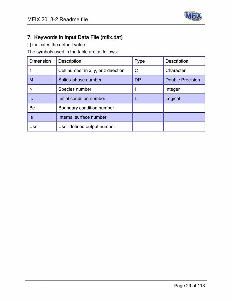
7. Keywords in Input Data File (mfix.dat) [ ] indicates the default value.
The symbols used in the table are as follows:
Dimension Description Type Description
1 Cell number in x, y, or z direction C Character
M Solids-phase number DP Double Precision
N Species number I Integer
Ic Initial condition number L Logical
Bc Boundary condition number
Is Internal surface number
Usr User-defined output number

MFIX 2013-2 Readme file
Page 30 of 113
7.1. Run Control
Keyword (dimension) Type Description
RUN_NAME C Name used to create output files. The name should be legal after extensions are added to it; e.g., for run name BUB01, the output files BUB01.LOG, BUB01.OUT, BUB01.RES, etc., will be created.
DESCRIPTION C Problem description in 60 characters.
UNITS C Units for data input and output.
[‘CGS’] All input and output in CGS units (g, cm, s, cal).
‘SI’ All input and output in SI units (kg, m, s, J).
RUN_TYPE C Type of run.
‘NEW’ New run.
‘RESTART_1’ Normal restart run. Initial conditions from .RES file.
‘RESTART_2’ Start a new run with initial conditions from a .RES file created from another run.
‘RESTART_3’ Continue old run as in RESTART_1, but any input data not given in mfix.dat is read from the .RES file. (Do not use)
‘RESTART_4’ Start a new run as in RESTART_2, but any input data not given in mfix.dat is read from the .RES file. (Do not use)
TIME DP Start-time of the run.
TSTOP DP Stop-time of the run.
DT DP Starting time step. If DT is not defined, a steady-state calculation will be performed.
DT_MAX
[1.0]
DP Maximum time step.
DT_MIN
[1E-6]
DP Minimum time step.
MFIX 2013-2 Readme file
Page 31 of 113
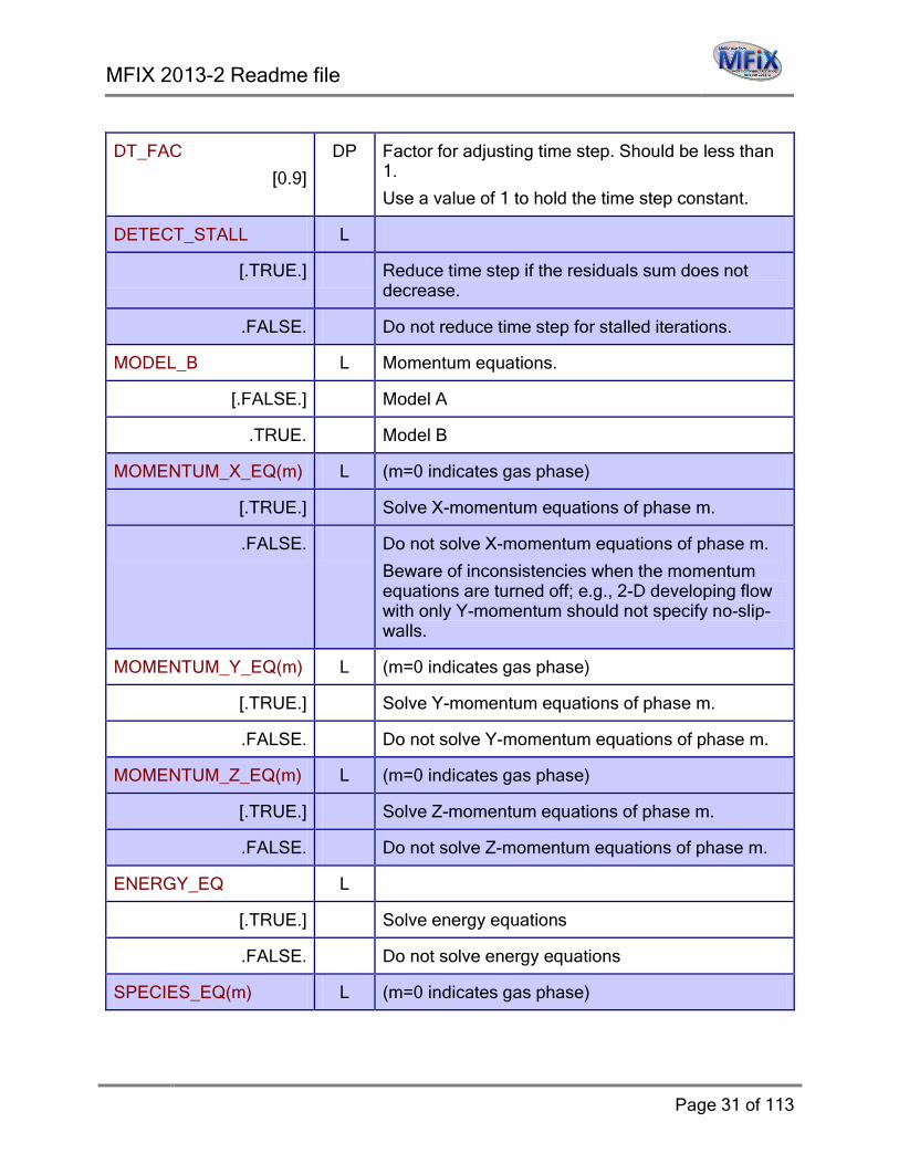
DT_FAC
[0.9]
DP Factor for adjusting time step. Should be less than 1.
Use a value of 1 to hold the time step constant.
DETECT_STALL L
[.TRUE.] Reduce time step if the residuals sum does not decrease.
.FALSE. Do not reduce time step for stalled iterations.
MODEL_B L Momentum equations.
[.FALSE.] Model A
.TRUE. Model B
MOMENTUM_X_EQ(m) L (m=0 indicates gas phase)
[.TRUE.] Solve X-momentum equations of phase m.
.FALSE. Do not solve X-momentum equations of phase m.
Beware of inconsistencies when the momentum equations are turned off; e.g., 2-D developing flow with only Y-momentum should not specify no-slip-walls.
MOMENTUM_Y_EQ(m) L (m=0 indicates gas phase)
[.TRUE.] Solve Y-momentum equations of phase m.
.FALSE. Do not solve Y-momentum equations of phase m.
MOMENTUM_Z_EQ(m) L (m=0 indicates gas phase)
[.TRUE.] Solve Z-momentum equations of phase m.
.FALSE. Do not solve Z-momentum equations of phase m.
ENERGY_EQ L
[.TRUE.] Solve energy equations
.FALSE. Do not solve energy equations
SPECIES_EQ(m) L (m=0 indicates gas phase)
MFIX 2013-2 Readme file
Page 32 of 113
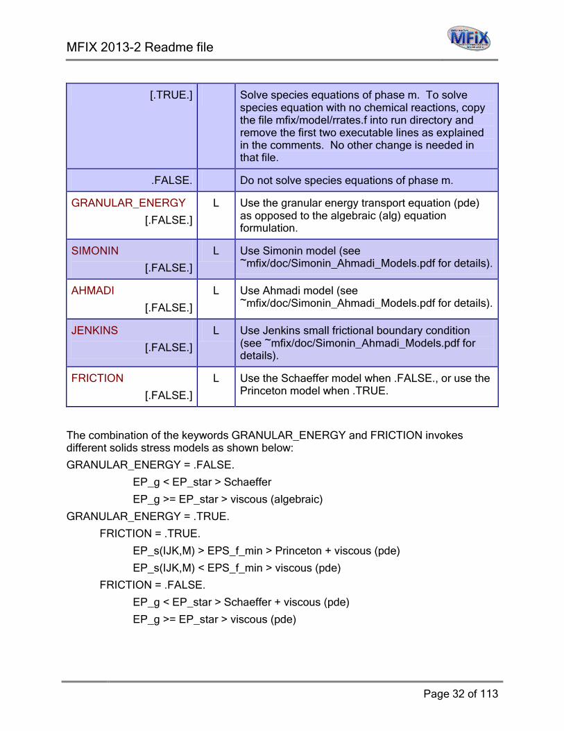
[.TRUE.] Solve species equations of phase m. To solve species equation with no chemical reactions, copy the file mfix/model/rrates.f into run directory and remove the first two executable lines as explained in the comments. No other change is needed in that file.
.FALSE. Do not solve species equations of phase m.
GRANULAR_ENERGY
[.FALSE.]
L Use the granular energy transport equation (pde) as opposed to the algebraic (alg) equation formulation.
SIMONIN
[.FALSE.]
L Use Simonin model (see ~mfix/doc/Simonin_Ahmadi_Models.pdf for details).
AHMADI
[.FALSE.]
L Use Ahmadi model (see ~mfix/doc/Simonin_Ahmadi_Models.pdf for details).
JENKINS
[.FALSE.]
L Use Jenkins small frictional boundary condition (see ~mfix/doc/Simonin_Ahmadi_Models.pdf for details).
FRICTION
[.FALSE.]
L Use the Schaeffer model when .FALSE., or use the Princeton model when .TRUE.
The combination of the keywords GRANULAR_ENERGY and FRICTION invokes different solids stress models as shown below:
GRANULAR_ENERGY = .FALSE.
EP_g < EP_star > Schaeffer
EP_g >= EP_star > viscous (algebraic)
GRANULAR_ENERGY = .TRUE.
FRICTION = .TRUE.
EP_s(IJK,M) > EPS_f_min > Princeton + viscous (pde)
EP_s(IJK,M) < EPS_f_min > viscous (pde)
FRICTION = .FALSE.
EP_g < EP_star > Schaeffer + viscous (pde)
EP_g >= EP_star > viscous (pde)
MFIX 2013-2 Readme file
Page 33 of 113
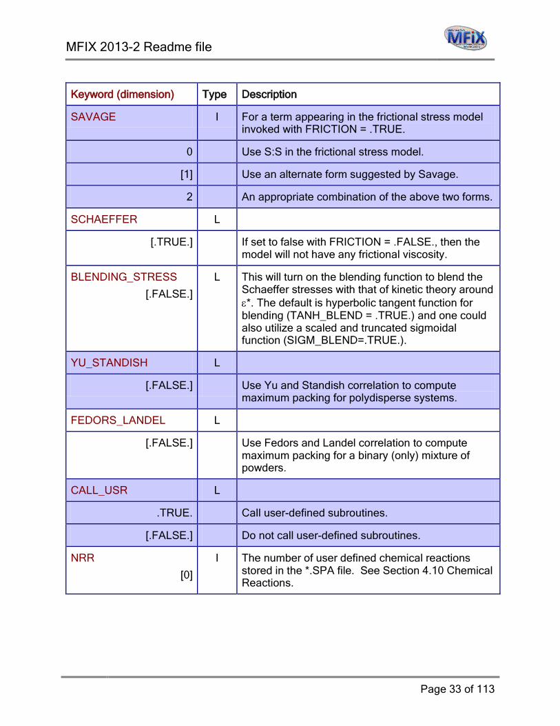
Keyword (dimension) Type Description
SAVAGE I For a term appearing in the frictional stress model invoked with FRICTION = .TRUE.
0 Use S:S in the frictional stress model.
[1] Use an alternate form suggested by Savage.
2 An appropriate combination of the above two forms.
SCHAEFFER L
[.TRUE.] If set to false with FRICTION = .FALSE., then the model will not have any frictional viscosity.
BLENDING_STRESS
[.FALSE.]
L This will turn on the blending function to blend the Schaeffer stresses with that of kinetic theory around ε*. The default is hyperbolic tangent function for blending (TANH_BLEND = .TRUE.) and one could also utilize a scaled and truncated sigmoidal function (SIGM_BLEND=.TRUE.).
YU_STANDISH L
[.FALSE.] Use Yu and Standish correlation to compute maximum packing for polydisperse systems.
FEDORS_LANDEL L
[.FALSE.] Use Fedors and Landel correlation to compute maximum packing for a binary (only) mixture of powders.
CALL_USR L
.TRUE. Call user-defined subroutines.
[.FALSE.] Do not call user-defined subroutines.
NRR
[0]
I The number of user defined chemical reactions stored in the *.SPA file. See Section 4.10 Chemical Reactions.
MFIX 2013-2 Readme file
Page 34 of 113
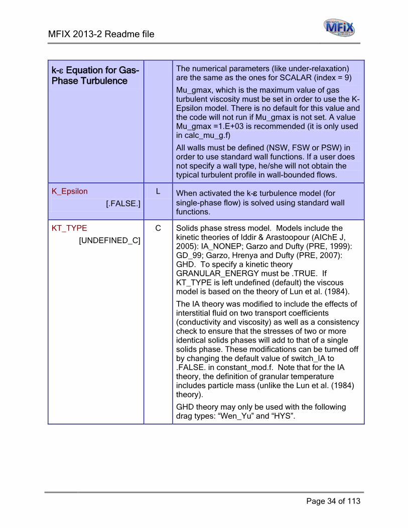
k-ε Equation for Gas-Phase Turbulence
The numerical parameters (like under-relaxation) are the same as the ones for SCALAR (index = 9)
Mu_gmax, which is the maximum value of gas turbulent viscosity must be set in order to use the K-Epsilon model. There is no default for this value and the code will not run if Mu_gmax is not set. A value Mu_gmax =1.E+03 is recommended (it is only used in calc_mu_g.f)
All walls must be defined (NSW, FSW or PSW) in order to use standard wall functions. If a user does not specify a wall type, he/she will not obtain the typical turbulent profile in wall-bounded flows.
K_Epsilon
[.FALSE.]
L When activated the k-ε turbulence model (for single-phase flow) is solved using standard wall functions.
KT_TYPE
[UNDEFINED_C]
C Solids phase stress model. Models include the kinetic theories of Iddir & Arastoopour (AIChE J, 2005): IA_NONEP; Garzo and Dufty (PRE, 1999): GD_99; Garzo, Hrenya and Dufty (PRE, 2007): GHD. To specify a kinetic theory GRANULAR_ENERGY must be .TRUE. If KT_TYPE is left undefined (default) the viscous model is based on the theory of Lun et al. (1984).
The IA theory was modified to include the effects of interstitial fluid on two transport coefficients (conductivity and viscosity) as well as a consistency check to ensure that the stresses of two or more identical solids phases will add to that of a single solids phase. These modifications can be turned off by changing the default value of switch_IA to .FALSE. in constant_mod.f. Note that for the IA theory, the definition of granular temperature includes particle mass (unlike the Lun et al. (1984) theory).
GHD theory may only be used with the following drag types: “Wen_Yu” and “HYS”.
MFIX 2013-2 Readme file
Page 35 of 113
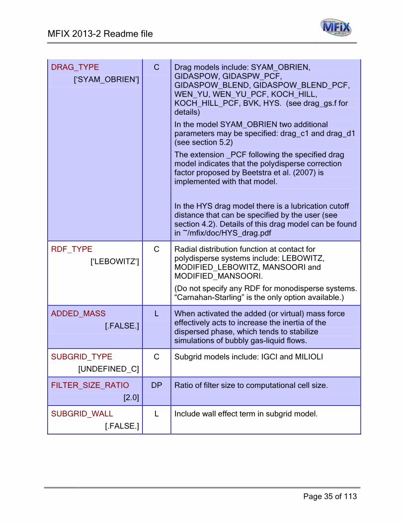
DRAG_TYPE
[‘SYAM_OBRIEN’]
C Drag models include: SYAM_OBRIEN, GIDASPOW, GIDASPW_PCF, GIDASPOW_BLEND, GIDASPOW_BLEND_PCF, WEN_YU, WEN_YU_PCF, KOCH_HILL, KOCH_HILL_PCF, BVK, HYS. (see drag_gs.f for details)
In the model SYAM_OBRIEN two additional parameters may be specified: drag_c1 and drag_d1 (see section 5.2)
The extension _PCF following the specified drag model indicates that the polydisperse correction factor proposed by Beetstra et al. (2007) is implemented with that model.
In the HYS drag model there is a lubrication cutoff distance that can be specified by the user (see section 4.2). Details of this drag model can be found in ~/mfix/doc/HYS_drag.pdf
RDF_TYPE
[‘LEBOWITZ‘]
C Radial distribution function at contact for polydisperse systems include: LEBOWITZ, MODIFIED_LEBOWITZ, MANSOORI and MODIFIED_MANSOORI.
(Do not specify any RDF for monodisperse systems. “Carnahan-Starling” is the only option available.)
ADDED_MASS
[.FALSE.]
L When activated the added (or virtual) mass force effectively acts to increase the inertia of the dispersed phase, which tends to stabilize simulations of bubbly gas-liquid flows.
SUBGRID_TYPE
[UNDEFINED_C]
C Subgrid models include: IGCI and MILIOLI
FILTER_SIZE_RATIO
[2.0]
DP Ratio of filter size to computational cell size.
SUBGRID_WALL
[.FALSE.]
L Include wall effect term in subgrid model.
MFIX 2013-2 Readme file
Page 36 of 113
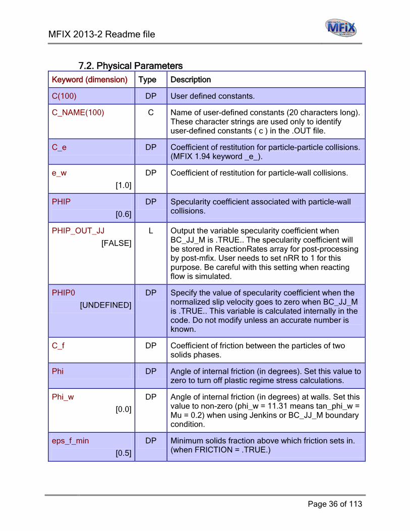
7.2. Physical Parameters
Keyword (dimension) Type Description
C(100) DP User defined constants.
C_NAME(100) C Name of user-defined constants (20 characters long). These character strings are used only to identify user-defined constants ( c ) in the .OUT file.
C_e DP Coefficient of restitution for particle-particle collisions. (MFIX 1.94 keyword _e_).
e_w
[1.0]
DP Coefficient of restitution for particle-wall collisions.
PHIP
[0.6]
DP Specularity coefficient associated with particle-wall collisions.
PHIP_OUT_JJ
[FALSE]
L Output the variable specularity coefficient when BC_JJ_M is .TRUE.. The specularity coefficient will be stored in ReactionRates array for post-processing by post-mfix. User needs to set nRR to 1 for this purpose. Be careful with this setting when reacting flow is simulated.
PHIP0
[UNDEFINED]
DP Specify the value of specularity coefficient when the normalized slip velocity goes to zero when BC_JJ_M is .TRUE.. This variable is calculated internally in the code. Do not modify unless an accurate number is known.
C_f DP Coefficient of friction between the particles of two solids phases.
Phi DP Angle of internal friction (in degrees). Set this value to zero to turn off plastic regime stress calculations.
Phi_w
[0.0]
DP Angle of internal friction (in degrees) at walls. Set this value to non-zero (phi_w = 11.31 means tan_phi_w = Mu = 0.2) when using Jenkins or BC_JJ_M boundary condition.
eps_f_min
[0.5]
DP Minimum solids fraction above which friction sets in. (when FRICTION = .TRUE.)

MFIX 2013-2 Readme file
Page 37 of 113
EP_S_MAX(MMAX)
[1.0 – ep_star]
DP Maximum solids volume fraction at packing for polydisperse systems (more than one solids phase used). The value of EP_star may change during the computation if solids phases with different particle diameters are specified and Yu_Standish or Fedors_Landel correlations are used.
SEGREGATION_SLOPE_COEFFICIENT
[0.0]
DP Used in calculating the initial slope of segregation: see Gera et al. (2004) - recommended value 0.3. Increasing this coefficient results in decrease in segregation of particles in binary mixtures.
L_scale0
[0.0]
DP Value of turbulent length initialized. This may be overwritten in specific regions with the keyword IC_L_scale.
Mu_gmax DP Maximum value of the turbulent viscosity of the fluid.
V_ex DP Excluded volume in Boyle-Massoudi stress.
[0.0] B-M stress is turned off.
P_ref
[0.0]
DP Reference pressure.
P_scale
[1.0]
DP Scale factor for pressure.
GRAVITY DP Gravitational acceleration.
[980.7] By default, the gravity force acts in the _ve y-direction. Modify file b_force2.inc to change the body force term.
drag_c1 and drag_d1
drag_c1 [0.8]
drag_d1 [2.65]
DP Quantities for calibrating Syamlal-O’Brien drag correlation using Umf data. These are determined using the Umf spreadsheet (http://www.mfix.org/members/develop/umf.xls). When these are undefined the default values for these constants are used.
USE_DEF_LAM_HYS
[.TRUE.]
L If set to .TRUE. MFIX will use default lubrication cutoff (LAM_HYS) of 1µm as specified in the drag_gs.f file for the HYS polydisperse drag model. If set to .FALSE. the user must specify a lubrication cutoff distance using the LAM_HYS keyword given in the next table entry.
MFIX 2013-2 Readme file
Page 38 of 113
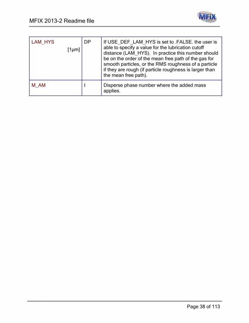
LAM_HYS
[1µm]
DP If USE_DEF_LAM_HYS is set to .FALSE. the user is able to specify a value for the lubrication cutoff distance (LAM_HYS). In practice this number should be on the order of the mean free path of the gas for smooth particles, or the RMS roughness of a particle if they are rough (if particle roughness is larger than the mean free path).
M_AM I Disperse phase number where the added mass applies.

MFIX 2013-2 Readme file
Page 39 of 113
7.3. Numerical Parameters
Keyword (dimension) Type Description
MAX_NIT
[500]
I Maximum number of iterations.
NORM_g
[Use the residual from the first iteration.]
DP Factor to normalize the gas continuity equation residual.
Setting Norm_g = 0 invokes a normalization method based on the dominant term in the continuity equation. This setting may speed up calculations, especially near a steady state and for incompressible fluids. But the number of pressure iterations may need to be increased, LEQ_IT(1), to ensure mass balance.
NORM_s
[Use the residual from the first iteration.]
DP Factor to normalize the solids continuity equation residual.
Setting Norm_s = 0 invokes a normalization method based on the dominant term in the continuity equation. This setting may speed up calculations, especially near a steady state. But the number of pressure iterations may need to be increased, LEQ_IT(2), to ensure mass balance.
TOL_RESID
[1E-3]
DP Maximum residual at convergence (continuity+momentum).
TOL_RESID_Th
[1E-4]
DP Maximum residual at convergence (granular energy).
TOL_RESID_T
[1E-4]
DP Maximum residual at convergence (energy).
TOL_RESID_X
[1E-4]
DP Maximum residual at convergence (species balance).
TOL_RESID_Scalar
[1E-4]
DP Maximum residual at convergence (scalar balances.)

MFIX 2013-2 Readme file
Page 40 of 113
TOL_DIVERGE
[1E+4]
DP Minimum residual for declaring divergence. When the fluid is incompressible, the velocity residuals take large values in the second iteration (e.g., 1E+8) and then drop down to a low value in the third iteration (e.g., 0.1). In such cases, it is desirable to increase this setting.
Max_Inlet_Vel_Fac
[1]
DP The code declares divergence if the velocity anywhere in the domain exceeds a maximum value. This maximum value is automatically determined from the boundary values. The user may scale the maximum value by adjusting this scale factor.
The next keywords LEQ_IT, LEQ_METHOD, LEQ_SWEEP, LEQ_TOL, UR_FAC, and DISCRETIZE are dimensioned for the nine types of equations:
Index Equation Type
1 gas pressure
2 solids volume fraction
3 gas and solids u-momentum
4 gas and solids v-momentum
5 gas and solids w-momentum
6 Temperature
7 species mass fractions
8 granular temperature
9 user-defined scalar
For example, LEQ_IT(3) = 10 will make MFIX use 10 linear equation iterations while solving the gas and solids u-momentum equation (Equation Type =3).

MFIX 2013-2 Readme file
Page 41 of 113
Keyword (dimension) Type Description
LEQ_IT(9)
[20 for 1 and 2]
[5 for 2-5]
[15 for 6-9]
I Number of iterations in the linear equation solver. The nine values are for the nine types of equations noted above.
The same convention holds for LEQ_METHOD, UR_FAC, and DISCRETIZE. If the residual of an equation is less than the convergence criterion, MFIX makes LEQ_IT equal to the lesser of 5 and the user-defined value and LEQ_METHOD equal to 1.
LEQ_METHOD(9)
[2 for all equations]
I The method used in the linear equation solver:
1. SOR
2. BiCGSTAB
3. GMRES
5. CG
LEQ_SWEEP(9)
[‘RSRS’]
C The sweep direction used in the linear equation solver. The sweep direction for preconditioning line relaxation; e.g., if LEQ_SWEEP = "ISIS", 1 sweep with do IK loop followed by send_recv (repeated twice), or if LEQ_SWEEP = "RSRS",1 red-black sweep with do IK loop followed by send_recv (repeated twice), or if LEQ_SWEEP = "ASAS",1 red-black sweep with do IK loop followed by do JK followed by IJ followed by send_recv (repeated twice). Only used by BiCGSTAB and CG.
LEQ_TOL(9)
[1.0D-4]
DP The tolerance, if used, in linear equation solvers. Only used by BiCGSTAB and CG.
LEQ_PC(9)
[LINE]
C The preconditioner used for the sweeps in the linear solver
LINE - Line relaxation
DIAG - Diagonal Scaling
NONE - No preconditioner

MFIX 2013-2 Readme file
Page 42 of 113
UR_FAC(9)
[0.8 for 1, 6, 9]
[0.5 for 2, 3, 4, 5, 8]
[1.0 for 7]
DP Under relaxation factors for seven types of equations.
Reducing UR_FAC(2) will help convergence in problems in which the solids tend to pack.
DEF_COR
[.FALSE.]
L If true, use deferred correction method for implementing higher order discretization. Otherwise, use down-wind factor method (default).
DISCRETIZE(9) I Discretization scheme for seven types of equations.
[0] First-order upwinding.
1 First-order upwinding (using down-wind factors).
2 Superbee (recommended method).
3 SMART.
4 ULTRA-QUICK.
5 QUICKEST (does not work).
6 MUSCL.
7 van Leer.
8 Minmod.
FPFOI
[.FALSE.]
L Four point fourth order interpolation and is upstream biased. If this scheme is chosen and discretize(*) < 2, discretize(*) is defaulted to 2. If you chose this scheme, set the C_FAC value between 0 and 1.
C_FAC
[UNDEFINED]
DP Factor used in the universal limiter (when FPFOI is set .TRUE.) and can be any value in the set (0,1). The choice of 1 will give (diffusion) first order upwinding and as this value becomes closer to 0 the scheme becomes more compressive.
CN_ON
[.FALSE.]
L Implicit Euler based temporal discretization scheme employed (first order accurate in time).
.TRUE. Crank-Nicholson based temporal discretization scheme employed (second order accurate in time excluding the restart timestep which is first order).
MFIX 2013-2 Readme file
Page 43 of 113
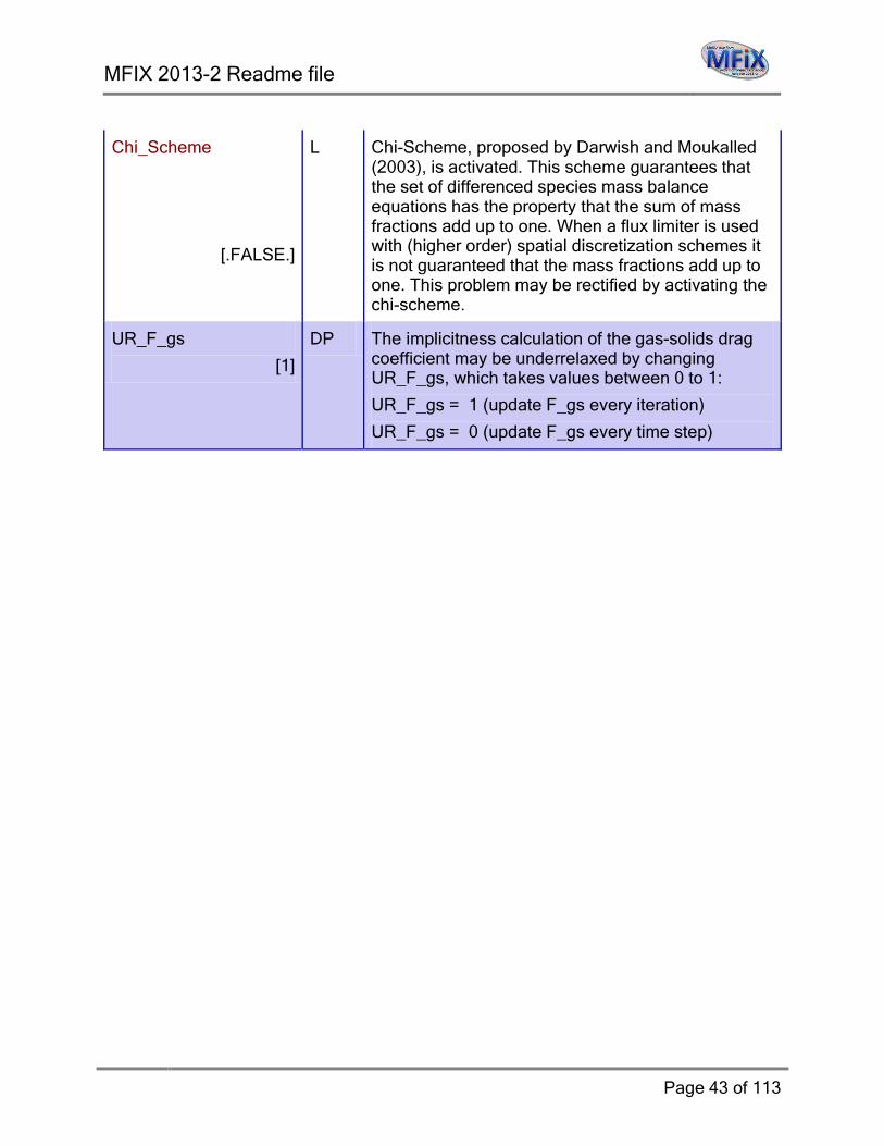
Chi_Scheme
[.FALSE.]
L Chi-Scheme, proposed by Darwish and Moukalled (2003), is activated. This scheme guarantees that the set of differenced species mass balance equations has the property that the sum of mass fractions add up to one. When a flux limiter is used with (higher order) spatial discretization schemes it is not guaranteed that the mass fractions add up to one. This problem may be rectified by activating the chi-scheme.
UR_F_gs
[1]
DP The implicitness calculation of the gas-solids drag coefficient may be underrelaxed by changing UR_F_gs, which takes values between 0 to 1:
UR_F_gs = 1 (update F_gs every iteration)
UR_F_gs = 0 (update F_gs every time step)
MFIX 2013-2 Readme file
Page 44 of 113
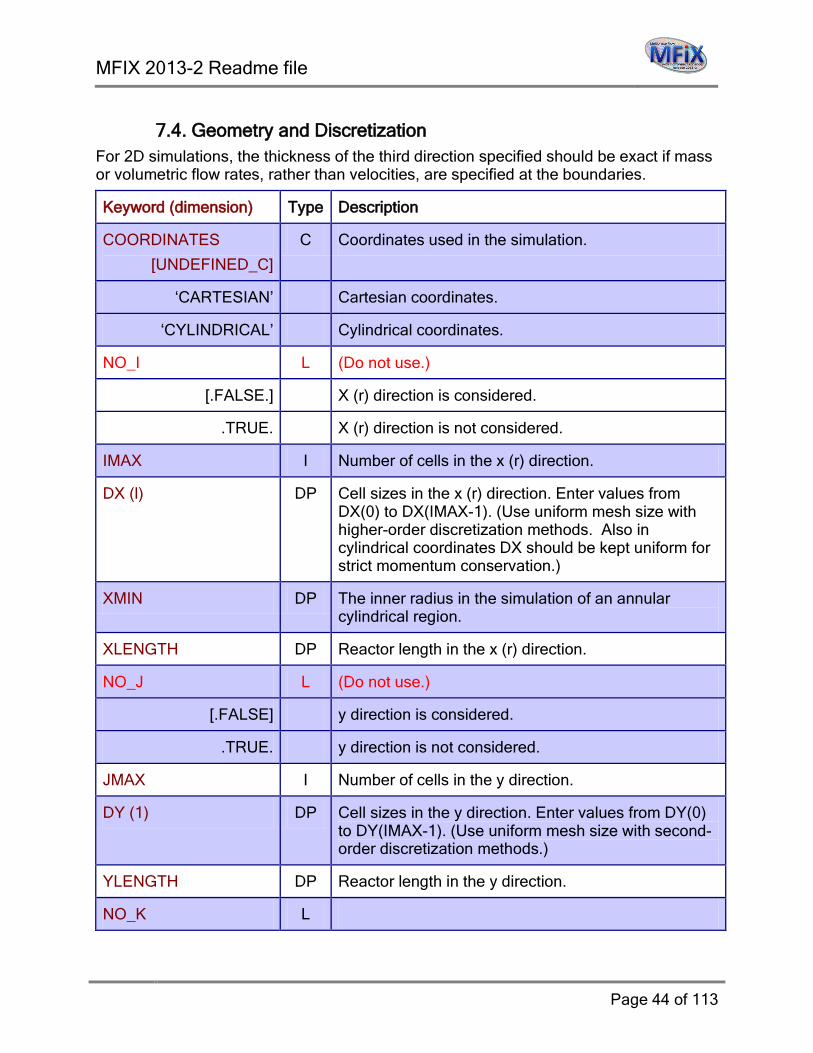
7.4. Geometry and Discretization For 2D simulations, the thickness of the third direction specified should be exact if mass or volumetric flow rates, rather than velocities, are specified at the boundaries.
Keyword (dimension) Type Description
COORDINATES
[UNDEFINED_C]
C Coordinates used in the simulation.
‘CARTESIAN’ Cartesian coordinates.
‘CYLINDRICAL’ Cylindrical coordinates.
NO_I L (Do not use.)
[.FALSE.] X (r) direction is considered.
.TRUE. X (r) direction is not considered.
IMAX I Number of cells in the x (r) direction.
DX (l) DP Cell sizes in the x (r) direction. Enter values from DX(0) to DX(IMAX-1). (Use uniform mesh size with higher-order discretization methods. Also in cylindrical coordinates DX should be kept uniform for strict momentum conservation.)
XMIN DP The inner radius in the simulation of an annular cylindrical region.
XLENGTH DP Reactor length in the x (r) direction.
NO_J L (Do not use.)
[.FALSE] y direction is considered.
.TRUE. y direction is not considered.
JMAX I Number of cells in the y direction.
DY (1) DP Cell sizes in the y direction. Enter values from DY(0) to DY(IMAX-1). (Use uniform mesh size with second-order discretization methods.)
YLENGTH DP Reactor length in the y direction.
NO_K L

MFIX 2013-2 Readme file
Page 45 of 113
[.FALSE.] z (θ) direction is considered.
.TRUE. z (θ) direction is not considered.
KMAX I Number of cells in the z (θ) direction.
DZ (1) DP Cell sizes in the z (θ) direction. Enter values from DZ(0) to DZ(IMAX-1). (Use uniform mesh size with second-order discretization methods.)
ZLENGTH DP Reactor length in the z (θdirection.
CYCLIC_X L Flag for making the x-direction cyclic without pressure drop. No other boundary conditions for the x-direction should be specified.
[.FALSE.] No cyclic condition at X-boundary.
.TRUE. Cyclic condition at X-boundary.
CYCLIC_X_PD L Flag for making the x-direction cyclic with pressure drop. If the keyword Flux_g is given a value this becomes a cyclic boundary condition with specified mass flux. No other boundary conditions for the x-direction should be specified.
[.FALSE.] No cyclic condition at X-boundary.
.TRUE. Cyclic condition with pressure drop at X-boundary.
DELP_X DP Fluid pressure drop across XLENGTH when a cyclic boundary condition with pressure drop is imposed in the x-direction.
CYCLIC_Y L Flag for making the y-direction cyclic without pressure drop. No other boundary conditions for the y-direction should be specified.
[.FALSE.] No cyclic condition at Y-boundary.
.TRUE. Cyclic condition at X-boundary.
CYCLIC_Y_PD L Flag for making the y-direction cyclic with pressure drop. If the keyword Flux_g is given a value this becomes a cyclic boundary condition with specified mass flux. No other boundary conditions for the y-direction should be specified.
MFIX 2013-2 Readme file
Page 46 of 113
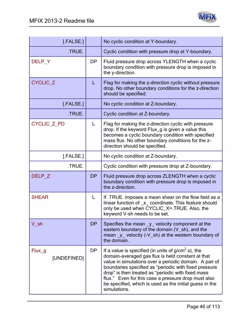
[.FALSE.] No cyclic condition at Y-boundary.
.TRUE. Cyclic condition with pressure drop at Y-boundary.
DELP_Y DP Fluid pressure drop across YLENGTH when a cyclic boundary condition with pressure drop is imposed in the y-direction.
CYCLIC_Z L Flag for making the z-direction cyclic without pressure drop. No other boundary conditions for the z-direction should be specified.
[.FALSE.] No cyclic condition at Z-boundary.
.TRUE. Cyclic condition at Z-boundary.
CYCLIC_Z_PD L Flag for making the z-direction cyclic with pressure drop. If the keyword Flux_g is given a value this becomes a cyclic boundary condition with specified mass flux. No other boundary conditions for the z-direction should be specified.
[.FALSE.] No cyclic condition at Z-boundary.
.TRUE. Cyclic condition with pressure drop at Z-boundary.
DELP_Z DP Fluid pressure drop across ZLENGTH when a cyclic boundary condition with pressure drop is imposed in the z-direction.
SHEAR L If .TRUE. imposes a mean shear on the flow field as a linear function of _x_ coordinate. This feature should only be used when CYCLIC_X=.TRUE. Also, the keyword V-sh needs to be set.
V_sh DP Specifies the mean _y_ velocity component at the eastern boundary of the domain (V_sh), and the mean _y_ velocity (-V_sh) at the western boundary of the domain.
Flux_g
[UNDEFINED]
DP If a value is specified (in units of g/cm2.s), the domain-averaged gas flux is held constant at that value in simulations over a periodic domain. A pair of boundaries specified as “periodic with fixed pressure drop” is then treated as “periodic with fixed mass flux.” Even for this case a pressure drop must also be specified, which is used as the initial guess in the simulations.

MFIX 2013-2 Readme file
Page 47 of 113
7.5. Gas Phase
Keyword (dimension) Type Description
RO_g0 DP Specified constant gas density. This value may be set to zero to make the drag zero and to simulate granular flow in a vacuum. For this case, users may turn off solving for gas momentum equations to accelerate convergence.
MU_g0 DP Specified constant gas viscosity.
K_g0 DP Specified constant gas conductivity.
C_pg0 DP Specified constant gas specific heat.
DIF_g0 DP Specified constant gas diffusivity.
MW_AVG DP Average molecular weight of gas.
MW_g (n) DP Molecular weight of gas species n.
7.6. Solids Phase Keyword (dimension) Type Description
MMAX
[1]
I Number of solids phases.
D_p0 (m) DP Initial particle diameters, same as the old D_P(m).
RO_s (m) DP Particle densities.
MU_s0 DP Specified constant granular viscosity. If this value is specified, then the kinetic theory calculation is turned off and P_s = 0 and Lambda_s = -2/3 MU_s0.
K_s0 DP Specified constant solids conductivity.
C_ps0 DP Specified constant solids specific heat.
DIF_s0 DP Specified constant solids diffusivity.
MW_s (m,n) DP Molecular weight of solids phase-m, species n.
MFIX 2013-2 Readme file
Page 48 of 113
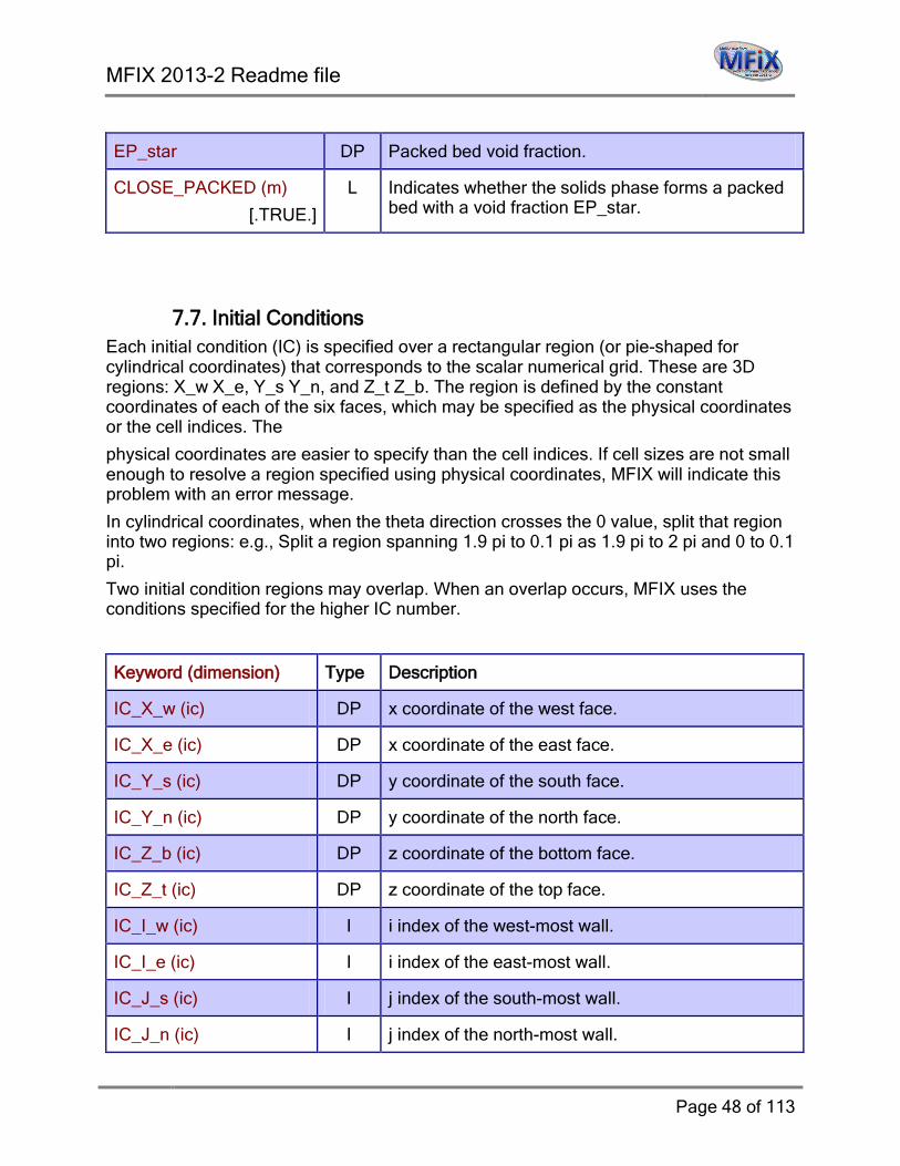
EP_star DP Packed bed void fraction.
CLOSE_PACKED (m)
[.TRUE.]
L Indicates whether the solids phase forms a packed bed with a void fraction EP_star.
7.7. Initial Conditions Each initial condition (IC) is specified over a rectangular region (or pie-shaped for cylindrical coordinates) that corresponds to the scalar numerical grid. These are 3D regions: X_w X_e, Y_s Y_n, and Z_t Z_b. The region is defined by the constant coordinates of each of the six faces, which may be specified as the physical coordinates or the cell indices. The
physical coordinates are easier to specify than the cell indices. If cell sizes are not small enough to resolve a region specified using physical coordinates, MFIX will indicate this problem with an error message.
In cylindrical coordinates, when the theta direction crosses the 0 value, split that region into two regions: e.g., Split a region spanning 1.9 pi to 0.1 pi as 1.9 pi to 2 pi and 0 to 0.1 pi.
Two initial condition regions may overlap. When an overlap occurs, MFIX uses the conditions specified for the higher IC number.
Keyword (dimension) Type Description
IC_X_w (ic) DP x coordinate of the west face.
IC_X_e (ic) DP x coordinate of the east face.
IC_Y_s (ic) DP y coordinate of the south face.
IC_Y_n (ic) DP y coordinate of the north face.
IC_Z_b (ic) DP z coordinate of the bottom face.
IC_Z_t (ic) DP z coordinate of the top face.
IC_I_w (ic) I i index of the west-most wall.
IC_I_e (ic) I i index of the east-most wall.
IC_J_s (ic) I j index of the south-most wall.
IC_J_n (ic) I j index of the north-most wall.

MFIX 2013-2 Readme file
Page 49 of 113
IC_K_b (ic) I k index of the bottom-most wall.
IC_K_t (ic) I k index of the top-most wall.
IC_TYPE (ic) C Type of initial condition. Mainly used in restart runs to overwrite values read from the .RES file by specifying it as _PATCH_. The user needs to be careful when using the _PATCH_ option, since the values from the .RES file are overwritten and no error checking is done for the patched values.
IC_EP_g (ic) DP Initial void fraction in the IC region.
IC_P_g (ic) DP Initial gas pressure in the IC region. If this quantity is not specified, MFIX will set up a hydrostatic pressure profile, which varies only in the y-direction.
IC_P_star (ic) DP Initial solids pressure in the IC region. Usually, this value is specified as zero.
IC_L_scale (ic) DP Turbulence length scale in the IC region.
IC_ROP_s (ic, m) DP Initial bulk density (rop_s = ro_s x ep_s) of solids phase-m in the IC region. Users need to specify this IC only for polydisperse flow (MMAX > 1). Users must make sure that summation of ( IC_ROP_s(ic,m) / RO_s(m) ) over all solids phases is equal to ( 1.0 – IC_EP_g(ic) ).
IC_T_g (ic) DP Initial gas phase temperature in the IC region.
IC_T_s (ic, m) DP Initial solids phase-m temperature in the IC region.
IC_Theta_m (ic, m) DP Initial solids phase-m granular temperature in the IC region.
IC_GAMA_Rg (ic)
[0]
DP Gas phase radiation coefficient in the IC region. Modify file radtn2.inc to change the source term.
IC_T_Rg (ic) DP Gas phase radiation temperature in the IC region.
IC_GAMA_Rs (ic, m)
[0]
DP Solids phase-m radiation coefficient in the IC region. Modify file radtn2.inc to change the source term.
IC_T_Rs (ic, m) DP Solids phase-m radiation temperature in the IC region.

MFIX 2013-2 Readme file
Page 50 of 113
IC_U_g (ic) DP Initial x-component of gas velocity in the IC region.
IC_U_s (ic, m) DP Initial x-component of solids-phase velocity in the IC region.
IC_V_g (ic) DP Initial y-component of gas velocity in the IC region.
IC_V_s (ic, m) DP Initial y-component of solids-phase velocity in the IC region.
IC_W_g (ic) DP Initial z-component of gas velocity in the IC region.
IC_W_s (ic, m) DP Initial z-component of solids-phase velocity in the IC region
IC_X_g (ic, n)
[0]
DP Initial mass fraction of gas species n.
IC_X_s (ic, m, n)
[0]
DP Initial mass fraction of solids phase-m, species n.
IC_SCALAR (ic, n)
[0]
DP Initial value of Scalar n.
MFIX 2013-2 Readme file
Page 51 of 113
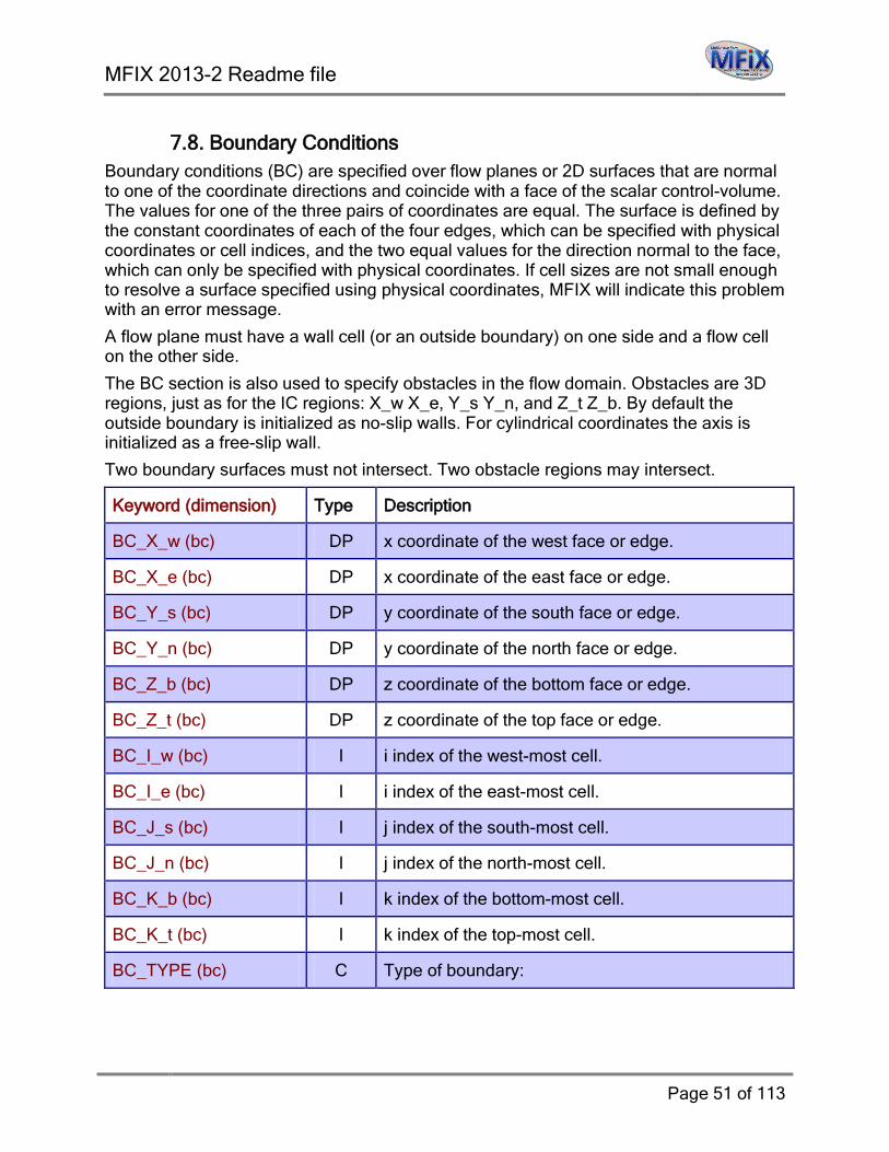
7.8. Boundary Conditions Boundary conditions (BC) are specified over flow planes or 2D surfaces that are normal to one of the coordinate directions and coincide with a face of the scalar control-volume. The values for one of the three pairs of coordinates are equal. The surface is defined by the constant coordinates of each of the four edges, which can be specified with physical coordinates or cell indices, and the two equal values for the direction normal to the face, which can only be specified with physical coordinates. If cell sizes are not small enough to resolve a surface specified using physical coordinates, MFIX will indicate this problem with an error message.
A flow plane must have a wall cell (or an outside boundary) on one side and a flow cell on the other side.
The BC section is also used to specify obstacles in the flow domain. Obstacles are 3D regions, just as for the IC regions: X_w X_e, Y_s Y_n, and Z_t Z_b. By default the outside boundary is initialized as no-slip walls. For cylindrical coordinates the axis is initialized as a free-slip wall.
Two boundary surfaces must not intersect. Two obstacle regions may intersect.
Keyword (dimension) Type Description
BC_X_w (bc) DP x coordinate of the west face or edge.
BC_X_e (bc) DP x coordinate of the east face or edge.
BC_Y_s (bc) DP y coordinate of the south face or edge.
BC_Y_n (bc) DP y coordinate of the north face or edge.
BC_Z_b (bc) DP z coordinate of the bottom face or edge.
BC_Z_t (bc) DP z coordinate of the top face or edge.
BC_I_w (bc) I i index of the west-most cell.
BC_I_e (bc) I i index of the east-most cell.
BC_J_s (bc) I j index of the south-most cell.
BC_J_n (bc) I j index of the north-most cell.
BC_K_b (bc) I k index of the bottom-most cell.
BC_K_t (bc) I k index of the top-most cell.
BC_TYPE (bc) C Type of boundary:

MFIX 2013-2 Readme file
Page 52 of 113
DUMMY The specified boundary condition is ignored. This is useful for turning off some boundary conditions without having to delete them from the file.
MASS_INFLOW or MI Mass inflow rates for gas and solids phases are specified at the boundary.
MASS_OUTFLOW or MO
The specified values of gas and solids mass outflow rates at the boundary are maintained, approximately. This condition should be used sparingly for minor outflows, when the bulk of the outflow is occurring through other constant pressure outflow boundaries.
P_INFLOW or PI Inflow from a boundary at a specified constant pressure. To specify as the west, south, or bottom end of the computational region, add a layer of wall cells to the west, south, or bottom of the PI cells. Users need to specify all scalar quantities and velocity components. The specified values of fluid and solids velocities are only used initially as MFIX computes these values at this inlet boundary.
P_OUTFLOW or PO Outflow to a boundary at a specified constant pressure. To specify as the west, south, or bottom end of the computational region, add a layer of wall cells to the west, south, or bottom of the PO cells.
FREE_SLIP_WALL or FSW
Velocity gradients at the wall vanish. If BC_JJ_PS is equal to 1, the Johnson-Jackson boundary condition is used for solids. A FSW is equivalent to using a PSW with hw=0.
NO_SLIP_WALL or NSW
All components of the velocity vanish at the wall. If BC_JJ_PS is equal to 1, the Johnson-Jackson boundary condition is used for solids. A NSW is equivalent to using a PSW with vw=0 and hw undefined.
MFIX 2013-2 Readme file
Page 53 of 113
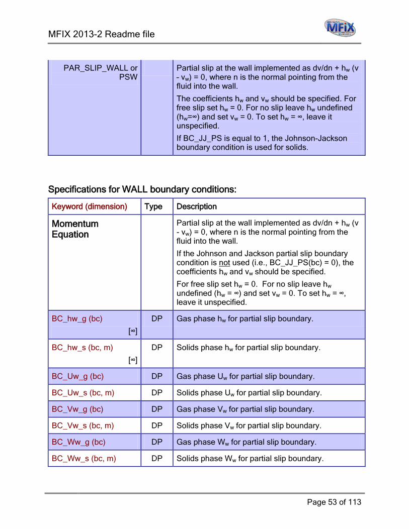
PAR_SLIP_WALL or PSW
Partial slip at the wall implemented as dv/dn + hw (v – vw) = 0, where n is the normal pointing from the fluid into the wall.
The coefficients hw and vw should be specified. For free slip set hw = 0. For no slip leave hw undefined (hw=∞) and set vw = 0. To set hw = ∞, leave it unspecified.
If BC_JJ_PS is equal to 1, the Johnson-Jackson boundary condition is used for solids.
Specifications for WALL boundary conditions:
Keyword (dimension) Type Description
Momentum Equation
Partial slip at the wall implemented as dv/dn + hw (v - vw) = 0, where n is the normal pointing from the fluid into the wall.
If the Johnson and Jackson partial slip boundary condition is not used (i.e., BC_JJ_PS(bc) = 0), the coefficients hw and vw should be specified.
For free slip set hw = 0. For no slip leave hw undefined (hw = ∞) and set vw = 0. To set hw = ∞, leave it unspecified.
BC_hw_g (bc)
[∞]
DP Gas phase hw for partial slip boundary.
BC_hw_s (bc, m)
[∞]
DP Solids phase hw for partial slip boundary.
BC_Uw_g (bc) DP Gas phase Uw for partial slip boundary.
BC_Uw_s (bc, m) DP Solids phase Uw for partial slip boundary.
BC_Vw_g (bc) DP Gas phase Vw for partial slip boundary.
BC_Vw_s (bc, m) DP Solids phase Vw for partial slip boundary.
BC_Ww_g (bc) DP Gas phase Ww for partial slip boundary.
BC_Ww_s (bc, m) DP Solids phase Ww for partial slip boundary.

MFIX 2013-2 Readme file
Page 54 of 113
BC_JJ_PS (bc) I 1: Use Johnson and Jackson partial slip bc. 0: Do not use Johnson and Jackson partial slip bc.
[0] If granular energy transport equation is not solved: (GRANULAR_ENERGY=.FALSE.).
[1] If granular energy transport equation is solved: (GRANULAR_ENERGY=.TRUE..
BC_JJ_M
[.FALSE.]
L Use the modified Johnson and Jackson partial slip BC with variable specularity coefficient. Must set e_w and phi_w with this BC.
Granular Energy Equation
The granular energy boundary condition is implemented as dT/dn + hw (T - Tw) = c, where n is the normal pointing from the fluid into the wall.
If the Johnson and Jackson partial slip boundary condition is not used (i.e., BC_JJ_PS(bc) = 0), the coefficients hw and c should be specified.
For specified heat flux set hw=0 and give a value for c. For specified temperature boundary condition leave hw unspecified (hw=∞ and give a value for Tw.
BC_Thetaw_m (bc, m) DP Tw for granular energy bc.
BC_hw_Theta_m (bc, m)
[∞]
DP Hw for granular energy bc.
BC_C_Theta_m (bc, m) DP c for granular energy bc.
Gas and Solids Energy Equations
The thermal boundary condition implemented as dT/dn + hw (T – Tw) = c, where n is the normal pointing from the fluid into the wall.
The coefficients hw, Tw, and c should be specified. Hw = 0 => specified heat flux; hw = ∞ => specified temperature boundary condition. To set hw = ∞ , leave it unspecified and give a value for Tw.
BC_hw_T_g (bc)
[ ]
DP Gas phase hw for heat transfer.
BC_hw_T_s (bc, m)
[∞]
DP Solids phase hw for heat transfer.

MFIX 2013-2 Readme file
Page 55 of 113
BC_Tw_g (bc) DP Gas phase Tw for heat transfer.
BC_Tw_s (bc, m) DP Solids phase Tw for heat transfer.
BC_C_T_g (bc) DP Gas phase C for heat transfer.
BC_C_T_s (bc, m) DP Solids phase C for heat transfer.
Gas and Solids Species Equations
The species diffusion boundary condition is implemented as dX/dn + hw (X - Xw) = c, where n is the normal pointing from the fluid into the wall.
The coefficients hw, Xw, and c should be specified. Hw = 0 => specified species diffusion flux; hw = ∞ => specified species concentration at the boundary. To set hw = ∞ , leave it unspecified and give a value for Xw.
BC_hw_X_g (bc, n)
[∞]
DP The species diffusion boundary condition is implemented as dX/dn + hw (X - Xw) = c, where n is the normal pointing from the fluid into the wall.
The coefficients hw, Xw, and c should be specified. Hw = 0 => specified species diffusion flux; hw = ∞ => specified species concentration at the boundary. To set hw = ∞ , leave it unspecified and give a value for Xw.
Gas phase hw for mass transfer.
BC_hw_X_s (bc, m, n)
[∞]
DP Solids phase hw for mass transfer.
BC_Xw_g (bc, n) DP Gas phase Xw for mass transfer.
BC_Xw_s (bc, m, n) DP Solids phase Xw for mass transfer.
BC_C_X_g (bc, n) DP Gas phase C for mass transfer.
BC_C_X_s (bc, m, n) DP Solids phase C for mass transfer.
Scalar Transport Equations
The scalar boundary condition is implemented as dS/dn + hw (S - Sw) = C, where n is the normal pointing from the fluid into the wall.
The coefficients hw, Sw, and c should be specified. Hw = 0 => specified species diffusion flux; hw = ∞ => specified species concentration at the boundary. To set hw = ∞ , leave it unspecified and give a value for Sw.
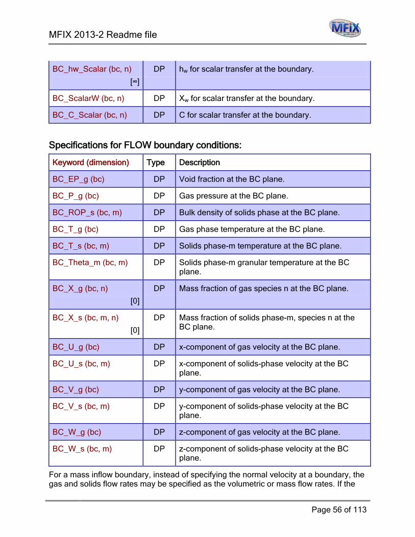
MFIX 2013-2 Readme file
Page 56 of 113
BC_hw_Scalar (bc, n)
[∞]
DP hw for scalar transfer at the boundary.
BC_ScalarW (bc, n) DP Xw for scalar transfer at the boundary.
BC_C_Scalar (bc, n) DP C for scalar transfer at the boundary.
Specifications for FLOW boundary conditions:
Keyword (dimension) Type Description
BC_EP_g (bc) DP Void fraction at the BC plane.
BC_P_g (bc) DP Gas pressure at the BC plane.
BC_ROP_s (bc, m) DP Bulk density of solids phase at the BC plane.
BC_T_g (bc) DP Gas phase temperature at the BC plane.
BC_T_s (bc, m) DP Solids phase-m temperature at the BC plane.
BC_Theta_m (bc, m) DP Solids phase-m granular temperature at the BC plane.
BC_X_g (bc, n)
[0]
DP Mass fraction of gas species n at the BC plane.
BC_X_s (bc, m, n)
[0]
DP Mass fraction of solids phase-m, species n at the BC plane.
BC_U_g (bc) DP x-component of gas velocity at the BC plane.
BC_U_s (bc, m) DP x-component of solids-phase velocity at the BC plane.
BC_V_g (bc) DP y-component of gas velocity at the BC plane.
BC_V_s (bc, m) DP y-component of solids-phase velocity at the BC plane.
BC_W_g (bc) DP z-component of gas velocity at the BC plane.
BC_W_s (bc, m) DP z-component of solids-phase velocity at the BC plane.
For a mass inflow boundary, instead of specifying the normal velocity at a boundary, the gas and solids flow rates may be specified as the volumetric or mass flow rates. If the

MFIX 2013-2 Readme file
Page 57 of 113
volumetric or mass flow rate is specified, MFIX will calculate the velocity normal to the boundary. The velocity calculated by MFIX, however, may differ from the velocity calculated based on the physical dimensions of the port because the simulated dimensions may not be exactly equal to the physical dimensions. Specify positive values for all the flow rates. MFIX will assign the correct sign to the computed velocity values.
If the mass or volumetric flow rate is specified for a mass outflow boundary condition, then at every interval BC_DT_0, MFIX will adjust the normal velocity so that the average computed-outflow rate is equal to the specified value. The user is cautioned, however, that if unrealistic mass flow rates are specified, the computations may become unstable. It is better to specify the velocity at the mass outflow boundary, if some amount of fluctuation in the mass outflow rate is tolerable.
Keyword (dimension) Type Description
BC_VOLFLOW_g (bc) DP Gas volumetric flow rate through the boundary.
BC_VOLFLOW_s (bc, m)
DP Solids volumetric flow rate through the boundary.
BC_MASSFLOW_g (bc)
DP Gas mass flow rate through the boundary.
BC_MASSFLOW_s (bc, m)
DP Solids mass flow rate through the boundary.
MFIX allows the specification of a transient jet with its velocity fluctuating between two values. The jet conditions will override the steady condition specified for the normal velocity. Therefore, if there is no transient jet, do not specify any of the following, except BC_DT_0, which may be required for mass outflow conditions.
Keyword (dimension) Type Description
BC_DT_0 (bc) DP The interval at the beginning when the normal velocity at the boundary is equal to BC_Jet_g0. When restarting, run this value and BC_Jet_g0 should be specified such that the transient jet continues correctly. MFIX does not store the jet conditions.
For MASS_OUTFLOW boundary conditions, BC_DT_0 is the time period to average and print the outflow rates. The adjustment of velocities to get a specified mass or volumetric flow rate is based on the average outflow rate.

MFIX 2013-2 Readme file
Page 58 of 113
BC_Jet_g0 DP Value of normal velocity during the initial interval BC_DT_0.
BC_DT_h (bc) DP The interval when normal velocity is equal to BC_Jet_gh.
BC_Jet_gh (bc) DP Value of normal velocity during the interval BC_DT_h.
BC_DT_1 (bc) DP The interval when normal velocity is equal to BC_Jet_g1.
BC_Jet_g1 (bc) DP Value of normal velocity during the interval BC_DT_1.

MFIX 2013-2 Readme file
Page 59 of 113
7.9. Internal Surfaces Internal surfaces (IS) are normal to one of the coordinate directions and coincide with one of the faces of the scalar control volume. One of the three pairs of coordinates is equal. The surface is defined by the constant coordinates of each of the four edges, which can be specified with physical coordinates or cell indices, and the two equal values for the direction normal to the face, which can only be specified with physical coordinates. If cell sizes are not small enough to resolve a surface specified using physical coordinates, MFIX will indicate this problem with an error message.
To specify a large number of internal surfaces in a region, a 3D region may be specified. When IS_Type is specified for such regions, add a prefix (X_, Y_, or Z_) to indicate the direction of the internal surfaces; e.g., X_IMPERMEABLE specifies impermeable internal surfaces parallel to the X coordinate.
Internal surfaces act as free-slip walls in stress computations. This default condition cannot be changed.
Keyword (dimension) Type Description
IS_X_w (is) DP x coordinate of the west face or edge.
IS_X_e (is) DP x coordinate of the east face or edge.
IS_Y_s (is) DP y coordinate of the south face or edge
IS_Y_n (is) DP y coordinate of the north face or edge
IS_Z_b (is) DP z coordinate of the bottom face or edge
IS_Z_t (is) DP z coordinate of the top face or edge
IS_I_w (is) I i index of the west-most cell.
IS_I_e (is) I i index of the east-most cell
IS_J_s (is) I j index of the south-most cell
IS_J_n (is) I j index of the north-most cell
IS_K_b (is) I k index of the bottom-most cell
IS_K_t (is) I k index of the top-most cell
IS_TYPE (is) C Type of internal surface:
IMPERMEABLE or IP No gas or solids flow through the surface.

MFIX 2013-2 Readme file
Page 60 of 113
SEMIPERMEABLE or SP
Gas flows through the surface with an additional resistance. Solids velocity through the surface is set to zero or to a user-specified fixed value (i.e., solids momentum equation for this direction is not solved)
IS_PC (is, 2)
(*, 1) = 1.E32
(*, 2) = 0.0
DP 1: permeability; 2: Inertial resistance coefficient. These values need to be specified for semipermeable surfaces only. The thickness used for pressure drop computation is that of the momentum cell (DX_e, DY_n, or DZ_t). To turn off the resistance, use a large value for permeability (1.E32) and a small value for the inertial resistance coefficient (0.0).
IS_VEL_S (is, m)
[0.0]
DP Value of fixed solids velocity through semipermeable surfaces.
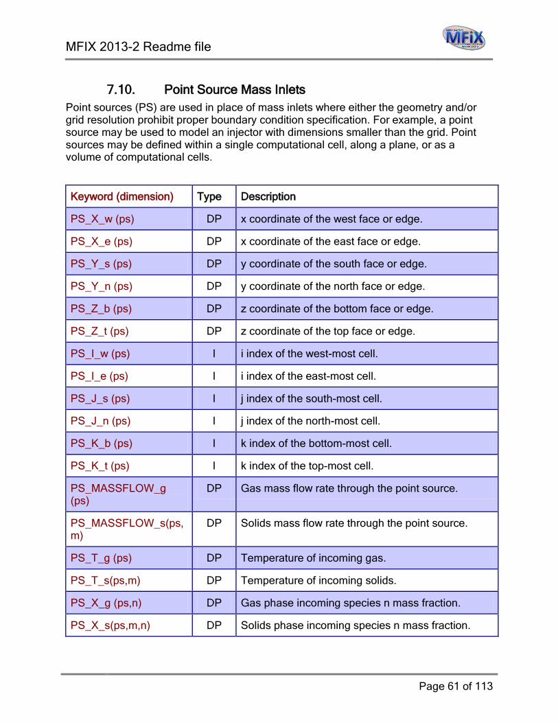
MFIX 2013-2 Readme file
Page 61 of 113
7.10. Point Source Mass Inlets Point sources (PS) are used in place of mass inlets where either the geometry and/or grid resolution prohibit proper boundary condition specification. For example, a point source may be used to model an injector with dimensions smaller than the grid. Point sources may be defined within a single computational cell, along a plane, or as a volume of computational cells.
Keyword (dimension) Type Description
PS_X_w (ps) DP x coordinate of the west face or edge.
PS_X_e (ps) DP x coordinate of the east face or edge.
PS_Y_s (ps) DP y coordinate of the south face or edge.
PS_Y_n (ps) DP y coordinate of the north face or edge.
PS_Z_b (ps) DP z coordinate of the bottom face or edge.
PS_Z_t (ps) DP z coordinate of the top face or edge.
PS_I_w (ps) I i index of the west-most cell.
PS_I_e (ps) I i index of the east-most cell.
PS_J_s (ps) I j index of the south-most cell.
PS_J_n (ps) I j index of the north-most cell.
PS_K_b (ps) I k index of the bottom-most cell.
PS_K_t (ps) I k index of the top-most cell.
PS_MASSFLOW_g (ps)
DP Gas mass flow rate through the point source.
PS_MASSFLOW_s(ps,m)
DP Solids mass flow rate through the point source.
PS_T_g (ps) DP Temperature of incoming gas.
PS_T_s(ps,m) DP Temperature of incoming solids.
PS_X_g (ps,n) DP Gas phase incoming species n mass fraction.
PS_X_s(ps,m,n) DP Solids phase incoming species n mass fraction.
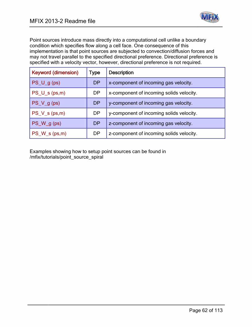
MFIX 2013-2 Readme file
Page 62 of 113
Point sources introduce mass directly into a computational cell unlike a boundary condition which specifies flow along a cell face. One consequence of this implementation is that point sources are subjected to convection/diffusion forces and may not travel parallel to the specified directional preference. Directional preference is specified with a velocity vector, however, directional preference is not required.
Keyword (dimension) Type Description
PS_U_g (ps) DP x-component of incoming gas velocity.
PS_U_s (ps,m) DP x-component of incoming solids velocity.
PS_V_g (ps) DP y-component of incoming gas velocity.
PS_V_s (ps,m) DP y-component of incoming solids velocity.
PS_W_g (ps) DP z-component of incoming gas velocity.
PS_W_s (ps,m) DP z-component of incoming solids velocity.
Examples showing how to setup point sources can be found in /mfix/tutorials/point_source_spiral

MFIX 2013-2 Readme file
Page 63 of 113
7.11. Output Control
Keyword (dimension) Type Description
RES_DT DP Interval at which restart (.RES) file is updated.
SPX_DT (11) DP Interval at which .SPX files are updated.
.SP1 Void fraction (EP_g).
.SP2 Gas pressure, solids pressure (P_g, P_star).
.SP3 Gas velocity (U_g, V_g, W_g).
.SP4 Solids velocity (U_s, V_s, W_s).
.SP5 Solids density (ROP_s).
.SP6 Gas and solids temperature (T_g, T_s1, T_s2).
.SP7 Gas and solids mass fractions (X_g, X-s).
.SP8 Granular temperature (G).
.SP9 User defined scalars.
.SPA Reaction Rates. (See section 4.11)
.SPB Turbulence quantities (k and ).
OUT_DT DP Interval at which standard output (.OUT) file is updated.
USR_DT (5) DP Interval at which user-defined outputs are written from the subroutine WRITE_USR1.
NLOG
[25]
I Interval in number of time steps at which .LOG file is written.
FULL_LOG
[.FALSE.]
L If true, display the residuals on the screen and messages about convergence on the screen and in the .LOG file.
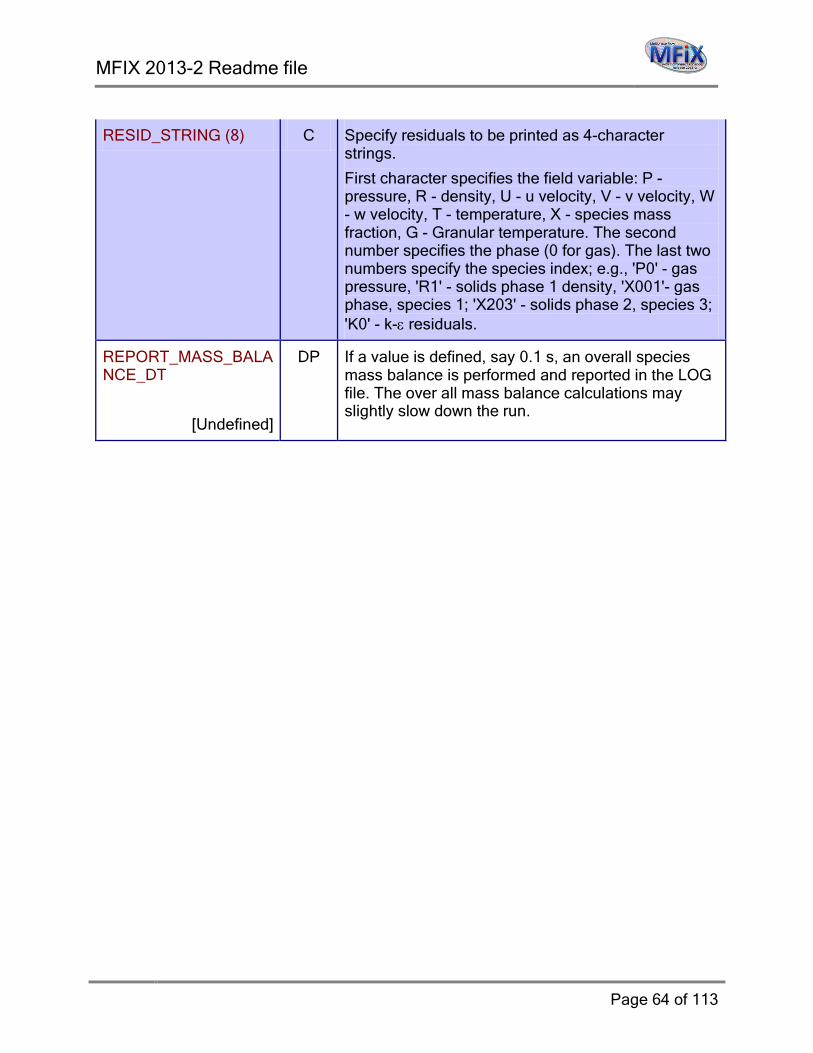
MFIX 2013-2 Readme file
Page 64 of 113
RESID_STRING (8) C Specify residuals to be printed as 4-character strings.
First character specifies the field variable: P - pressure, R - density, U - u velocity, V - v velocity, W - w velocity, T - temperature, X - species mass fraction, G - Granular temperature. The second number specifies the phase (0 for gas). The last two numbers specify the species index; e.g., 'P0' - gas pressure, 'R1' - solids phase 1 density, 'X001'- gas phase, species 1; 'X203' - solids phase 2, species 3; 'K0' - k-ε residuals.
REPORT_MASS_BALANCE_DT
[Undefined]
DP If a value is defined, say 0.1 s, an overall species mass balance is performed and reported in the LOG file. The over all mass balance calculations may slightly slow down the run.
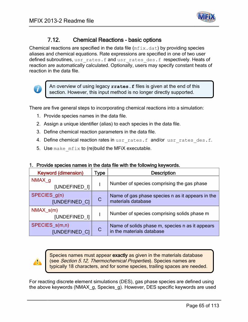
MFIX 2013-2 Readme file
Page 65 of 113
7.12. Chemical Reactions – basic options Chemical reactions are specified in the data file (mfix.dat) by providing species aliases and chemical equations. Rate expressions are specified in one of two user defined subroutines, usr_rates.f and usr_rates_des.f respectively. Heats of reaction are automatically calculated. Optionally, users may specify constant heats of reaction in the data file.
There are five general steps to incorporating chemical reactions into a simulation:
1. Provide species names in the data file.
2. Assign a unique identifier (alias) to each species in the data file.
3. Define chemical reaction parameters in the data file.
4. Define chemical reaction rates in usr_rates.f and/or usr_rates_des.f.
5. Use make_mfix to (re)build the MFiX executable. 1. Provide species names in the data file with the following keywords.
Keyword (dimension) Type Description
NMAX_g [UNDEFINED_I] I Number of species comprising the gas phase
SPECIES_g(n) [UNDEFINED_C] C
Name of gas phase species n as it appears in the materials database
NMAX_s(m) [UNDEFINED_I] I Number of species comprising solids phase m
SPECIES_s(m,n) [UNDEFINED_C] C
Name of solids phase m, species n as it appears in the materials database
For reacting discrete element simulations (DES), gas phase species are defined using the above keywords (NMAX_g, Species_g). However, DES specific keywords are used
Species names must appear exactly as given in the materials database (see Section 5.12, Thermochemical Properties). Species names are typically 18 characters, and for some species, trailing spaces are needed.
An overview of using legacy rrates.f files is given at the end of this section. However, this input method is no longer directly supported.

MFIX 2013-2 Readme file
Page 66 of 113
to identify the number of discrete solids phase species and material database names.
Keyword (dimension) Type Description
DES_NMAX_s(m) [UNDEFINED_I]
I Number of species comprising discrete solids phase m
DES_SPECIES_s(m,n) [UNDEFINED_C]
C Name of discrete solids phase m, species n as it appears in the materials database
2. Assign a unique identifier (alias) to each species with the following keyworks.
Keyword (dimension) Type Description
SPECIES_ALIAS_g(n) [UNDEFINED_C] C User defined name for gas phase species n
SPECIES_ALIAS_s(m,n) [UNDEFINED_C] C User defined name for solids phase m, species n
DES_SPECIES_ALIAS_s (m,n)
[UNDEFINED_C] C
User defined name for discrete solids phase m, species n
Alias formatting restrictions: • Aliases must be unique. • Aliases are limited to 32 characters and must follow FORTRAN variable naming
conventions (i.e., alphanumeric combinations with a letter as the first character). • Aliases are not case sensitive. • Aliases cannot conflict with existing MFiX variable names (e.g., a species alias of
MU_g will cause an error when compiling MFiX).
3. Define chemical reactions in the data file using species aliases.
Each reaction is identified by a reaction construct, and a reaction block is used to group reaction constructs in the data file. A reaction construct has the format, rxn_name{…}, where rxn_name is a unique identifier for the reaction. Reaction identifiers are limited to 32 characters and must follow FORTRAN variable naming convention.

MFIX 2013-2 Readme file
Page 67 of 113
There are two reaction block types:
@(RXNS)…@(END) – indicates continuum phase chemical reactions (all TFM gas and solids phase reactions and DES homogeneous gas phase reactions).
@(DES_RXNS)…@(DES_END) – indicates heterogeneous DES chemical reactions (particle/gas).
The following keywords are available within a reaction construct.
Keyword (dimension) Type Description
CHEM_EQ
[UNDEFINED_C]
C
Chemical equation for the reaction constructed from species aliases.
Ex: Char combustion
CHEM_EQ = “C + 0.5O2 --> CO”
DH (†Optional) [UNDEFINED] DP
User provided heat of reaction (cal/ mole for CGS and J/kmole for SI).
fracDH(m) (†Optional) [ZERO] DP The fractional amount of DH supplied to phase m.
* A chemical reaction equation of “NONE” deactivates the reaction during a simulation (e.g., CHEM_EQ = “NONE”).
† By default, heats of reaction are automatically calculated and assigned to the appropriate phase(s). However, users may specify a constant heat of reaction,
A data file can only contain one reaction block of each type, whereas a reaction block must contain one or more reaction constructs.
MFiX processes chemical reaction data differently than other input in the data file. A reaction block indicates the start and end of the reaction input. A reaction construct groups a single reaction’s input parameters.
@(RXNS) rxn1 { <input parameters> } rxn2 { <input parameters> } @(END)
reaction construct
reaction block
reaction construct
reaction identifiers
mfix.dat reaction input
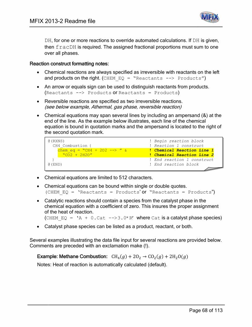
MFIX 2013-2 Readme file
Page 68 of 113
DH, for one or more reactions to override automated calculations. If DH is given, then fracDH is required. The assigned fractional proportions must sum to one over all phases.
Reaction construct formatting notes:
• Chemical reactions are always specified as irreversible with reactants on the left and products on the right. (CHEM_EQ = “Reactants --> Products”)
• An arrow or equals sign can be used to distinguish reactants from products. (Reactants --> Products or Reactants = Products)
• Reversible reactions are specified as two irreversible reactions. (see below example, Athermal, gas phase, reversible reaction)
• Chemical equations may span several lines by including an ampersand (&) at the end of the line. As the example below illustrates, each line of the chemical equation is bound in quotation marks and the ampersand is located to the right of the second quotation mark. hidden text
• Chemical equations are limited to 512 characters.
• Chemical equations can be bound within single or double quotes. (CHEM_EQ = ‘Reactants = Products’ or “Reactants = Products”)
• Catalytic reactions should contain a species from the catalyst phase in the chemical equation with a coefficient of zero. This insures the proper assignment of the heat of reaction. (CHEM_EQ = ‘A + 0.Cat -->3.0*R’ where Cat is a catalyst phase species)
• Catalyst phase species can be listed as a product, reactant, or both.
Several examples illustrating the data file input for several reactions are provided below. Comments are preceded with an exclamation make (!).
Example: Methane Combustion: CH4(𝑔) + 2O2 → CO2(𝑔) + 2H2O(𝑔)
Notes: Heat of reaction is automatically calculated (default).
@(RXNS) ! Begin reaction block CH4_Combustion { ! Reaction 1 construct chem_eq = “CH4 + 2O2 --> ” & ! Chemical Reaction Line 1 “CO2 + 2H2O” ! Chemical Reaction Line 2 } ! End reaction 1 construct @(END) ! End reaction block
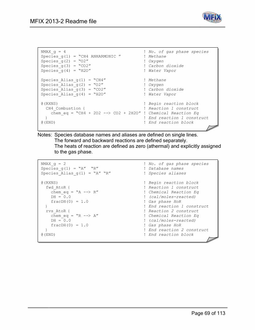
MFIX 2013-2 Readme file
Page 69 of 113
Example: Athermal, gas phase, reversible reaction: A(𝑔) ↔ R(𝑔)
Notes: Species database names and aliases are defined on single lines. The forward and backward reactions are defined separately. The heats of reaction are defined as zero (athermal) and explicitly assigned to the gas phase.
NMAX_g = 2 ! No. of gas phase species Species_g(1) = “A” “R” ! Database names Species_Alias_g(1) = “A” “R” ! Species aliases @(RXNS) ! Begin reaction block fwd_AtoR { ! Reaction 1 construct chem_eq = “A --> R” ! Chemical Reaction Eq DH = 0.0 ! (cal/moles-reacted) fracDH(0) = 1.0 ! Gas phase HoR } ! End reaction 1 construct rvs_AtoR { ! Reaction 2 construct chem_eq = “R --> A” ! Chemical Reaction Eq DH = 0.0 ! (cal/moles-reacted) fracDH(0) = 1.0 ! Gas phase HoR } ! End reaction 2 construct @(END) ! End reaction block
NMAX_g = 4 ! No. of gas phase species Species_g(1) = “CH4 ANHARMONIC ” ! Methane Species_g(2) = “O2” ! Oxygen Species_g(3) = “CO2” ! Carbon dioxide Species_g(4) = “H2O” ! Water Vapor Species_Alias_g(1) = “CH4” ! Methane Species_Alias_g(2) = “O2” ! Oxygen Species_Alias_g(3) = “CO2” ! Carbon dioxide Species_Alias_g(4) = “H2O” ! Water Vapor @(RXNS) ! Begin reaction block CH4_Combustion { ! Reaction 1 construct chem_eq = “CH4 + 2O2 --> CO2 + 2H2O” ! Chemical Reaction Eq } ! End reaction 1 construct @(END) ! End reaction block

MFIX 2013-2 Readme file
Page 70 of 113
Example - Char combustion: C(𝑠) + 0.5O2(𝑔) → CO(𝑔)
Notes: Species database names and aliases are defined on single lines. The heat of reaction is defined. The gas phase receives 20% of the heat of reaction. Solids phase 1 receives 80% of the heat of reaction.
NMAX_g = 2 ! No. gas phase species Species_g(1) = “O2” “CO” ! Database names Species_Alias_g(1) = “O2” “CO” ! Species aliases NMAX_s(1) = 2 ! No. solids phase species Species_s(1,1) = “C(GR) REF ELEMENT” ! Fixed Carbon (graphite) Species_s(1,2) = “Coal Ash” ! Coal Ash Species_Alias_s(1,1) = “C” “Ash” ! Fixed Carbon and Coal Ash @(RXNS) ! Begin reaction block Char_Combustion { ! Reaction 1 construct chem_eq = “C + 0.5O2 --> CO” ! Chemical Reaction Eq DH = -52834.0 ! (cal/moles-reacted) fracDH(0) = 0.2 ! HoR assigned to gas phase fracDH(1) = 0.8 ! HoR assigned to s. phase 1 } ! End reaction 1 construct @(END) ! End reaction block

MFIX 2013-2 Readme file
Page 71 of 113
Example – Compound DEM reaction:
CO combustion: CO(𝑔) + 0.5O2(𝑔) → CO2(𝑔)
CO2 gasification: C(𝑠) + CO2(𝑔) → 2CO(𝑔)
Char combustion: C(𝑠) + 0.5O2(𝑔) → CO(𝑔)
Notes: Gas phase species names and aliases are defined on the same line. DES specific keywords are used to defined DES species data. Heats of reaction for all reactions are calculated automatically. A TFM reaction block is used for the gas phase homogeneous reaction. A DEM reaction block is used for gas/solids reactions. Reaction constructs are given in one line.
Additional comments:
• Coal Ash is not a species included in the thermochemical database and would require that the properties be given in the data file (see Section 5.12 Thermochemical properties).
• One-line reaction constructs are only possible when the heat of reaction is automatically calculated (i.e., the chemical equation is the only input parameter).
! Gas phase species data NMAX_g = 3 Species_g(1) = “O2” Species_Alias_g(1) = “O2” Species_g(2) = “CO” Species_Alias_g(2) = “CO” Species_g(3) = “CO2” Species_Alias_g(3) = “CO2” ! DES solids phase species data DES_NMAX_s(1) = 2 DES_Species_s(1,1) = “C(GR) REF ELEMENT” DES_Species_s(1,2) = “Coal Ash” DES_Species_Alias_s(1,1) = “C” DES_Species_Alias_s(1,2) = “Ash” ! Homogeneous gas phase reactions @(RXNS) CO_Combustion { chem_eq = “CO + 0.5O2 --> CO2” } @(END) ! DES Reaction block @(DES_RXNS) CO2_Gasification { chem_eq = “2.0C + O2 --> 2CO” } Char_Combustion { chem_eq = “C + CO2 --> 2CO” } @(DES_END)
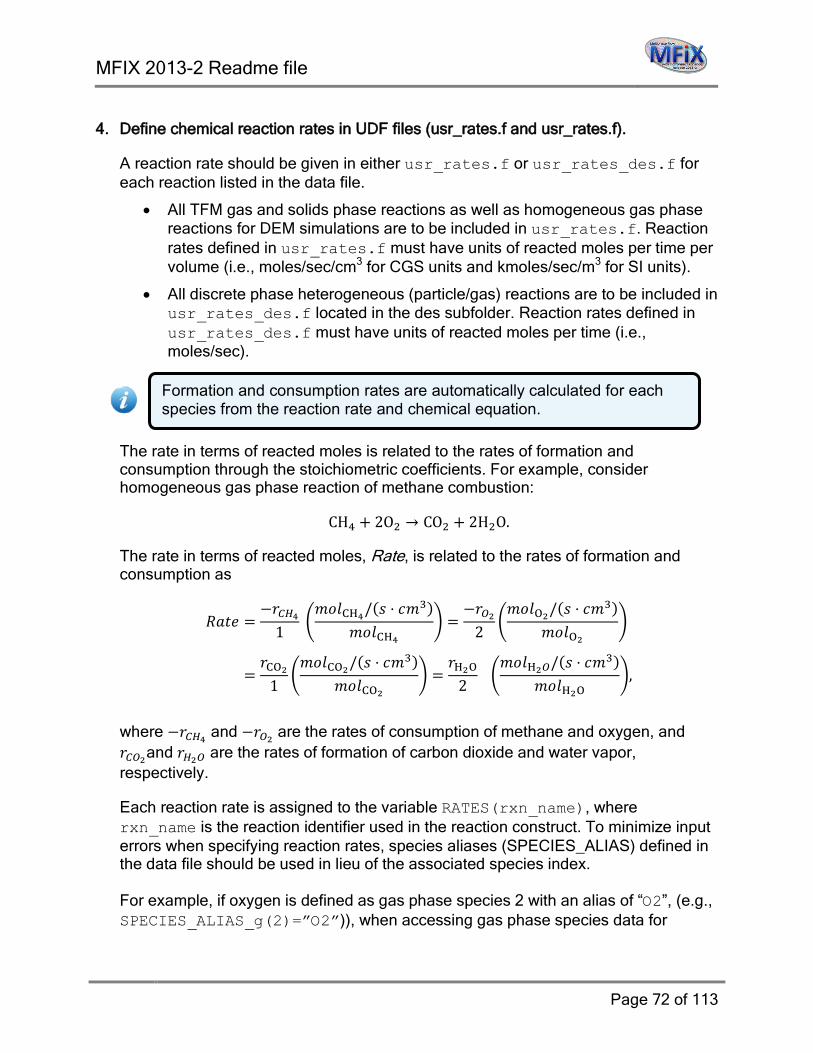
MFIX 2013-2 Readme file
Page 72 of 113
4. Define chemical reaction rates in UDF files (usr_rates.f and usr_rates.f).
A reaction rate should be given in either usr_rates.f or usr_rates_des.f for each reaction listed in the data file.
• All TFM gas and solids phase reactions as well as homogeneous gas phase reactions for DEM simulations are to be included in usr_rates.f. Reaction rates defined in usr_rates.f must have units of reacted moles per time per volume (i.e., moles/sec/cm3 for CGS units and kmoles/sec/m3 for SI units).
• All discrete phase heterogeneous (particle/gas) reactions are to be included in usr_rates_des.f located in the des subfolder. Reaction rates defined in usr_rates_des.f must have units of reacted moles per time (i.e., moles/sec).
The rate in terms of reacted moles is related to the rates of formation and consumption through the stoichiometric coefficients. For example, consider homogeneous gas phase reaction of methane combustion:
CH4 + 2O2 → CO2 + 2H2O.
The rate in terms of reacted moles, Rate, is related to the rates of formation and consumption as
𝑅𝑎𝑡𝑒 =−𝑟𝐶𝐻4
1 �𝑚𝑜𝑙CH4/(𝑠 ⋅ 𝑐𝑚3)
𝑚𝑜𝑙CH4� =
−𝑟𝑂22
�𝑚𝑜𝑙O2/(𝑠 ⋅ 𝑐𝑚3)
𝑚𝑜𝑙O2�
=𝑟CO2
1�𝑚𝑜𝑙CO2/(𝑠 ⋅ 𝑐𝑚3)
𝑚𝑜𝑙CO2� =
𝑟H2O2
�𝑚𝑜𝑙H2𝑂/(𝑠 ⋅ 𝑐𝑚3)
𝑚𝑜𝑙H2O�,
where −𝑟𝐶𝐻4 and −𝑟𝑂2 are the rates of consumption of methane and oxygen, and 𝑟𝐶𝑂2and 𝑟𝐻2𝑂 are the rates of formation of carbon dioxide and water vapor, respectively.
Each reaction rate is assigned to the variable RATES(rxn_name), where rxn_name is the reaction identifier used in the reaction construct. To minimize input errors when specifying reaction rates, species aliases (SPECIES_ALIAS) defined in the data file should be used in lieu of the associated species index. For example, if oxygen is defined as gas phase species 2 with an alias of “O2”, (e.g., SPECIES_ALIAS_g(2)=”O2”)), when accessing gas phase species data for
Formation and consumption rates are automatically calculated for each species from the reaction rate and chemical equation.
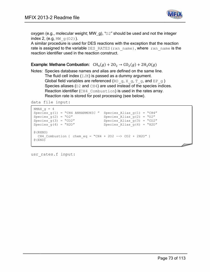
MFIX 2013-2 Readme file
Page 73 of 113
oxygen (e.g., molecular weight; MW_g), “O2” should be used and not the integer index 2, (e.g, MW_g(O2)). A similar procedure is used for DES reactions with the exception that the reaction rate is assigned to the variable DES_RATES(rxn_name), where rxn_name is the reaction identifier used in the reaction construct.
Example: Methane Combustion: CH4(𝑔) + 2O2 → CO2(𝑔) + 2H2O(𝑔)
Notes: Species database names and alias are defined on the same line. The fluid cell index (IJK) is passed as a dummy argument. Global field variables are referenced (RO_g, X_g, T_g, and EP_g ) Species aliases (O2 and CH4) are used instead of the species indices. Reaction identifier (CH4_Combustion) is used in the rates array. Reaction rate is stored for post processing (see below).
data file input:
usr_rates.f input:
NMAX_g = 4 Species_g(1) = “CH4 ANHARMONIC ” Species_Alias_g(1) = “CH4” Species_g(2) = “O2” Species_Alias_g(2) = “O2” Species_g(3) = “CO2” Species_Alias_g(3) = “CO2” Species_g(4) = “H2O” Species_Alias_g(4) = “H2O” @(RXNS) CH4_Combustion { chem_eq = “CH4 + 2O2 --> CO2 + 2H2O” } @(END)
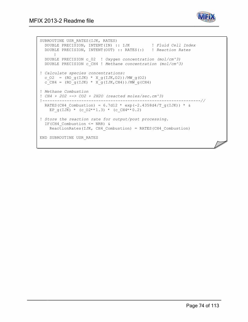
MFIX 2013-2 Readme file
Page 74 of 113
SUBROUTINE USR_RATES(IJK, RATES) DOUBLE PRECISION, INTENT(IN) :: IJK ! Fluid Cell Index DOUBLE PRECISION, INTENT(OUT) :: RATES(:) ! Reaction Rates ⋮ DOUBLE PRECISION c_02 ! Oxygen concentration (mol/cm^3) DOUBLE PRECISION c_CH4 ! Methane concentration (mol/cm^3) ! Calculate species concentrations: c_O2 = (RO_g(IJK) * X_g(IJK,O2))/MW_g(O2) c_CH4 = (RO_g(IJK) * X_g(IJK,CH4))/MW_g(CH4) ! Methane Combustion ! CH4 + 2O2 --> CO2 + 2H2O (reacted moles/sec.cm^3) !-----------------------------------------------------------------// RATES(CH4_Combustion) = 6.7d12 * exp(-2.4358d4/T_g(IJK)) * & EP_g(IJK) * (c_O2**1.3) * (c_CH4**0.2) ! Store the reaction rate for output/post processing. IF(CH4_Combustion <= NRR) & ReactionRates(IJK, CH4_Combustion) = RATES(CH4_Combustion) END SUBROUTINE USR_RATES
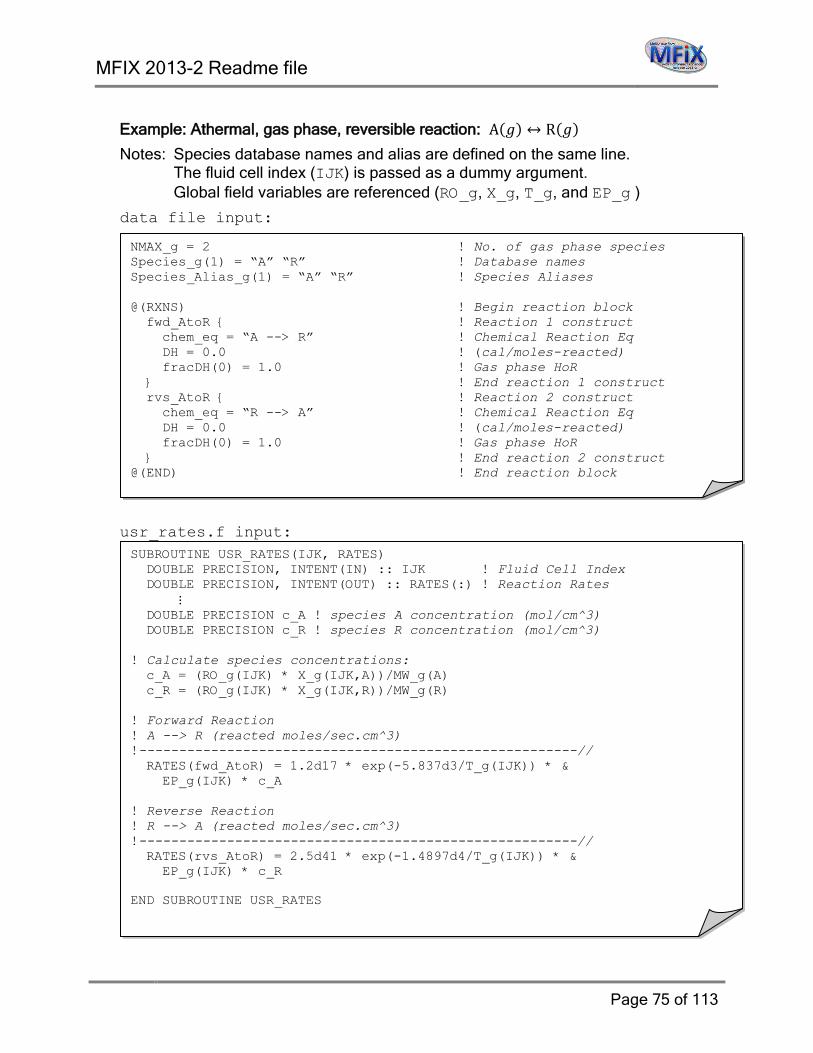
MFIX 2013-2 Readme file
Page 75 of 113
Example: Athermal, gas phase, reversible reaction: A(𝑔) ↔ R(𝑔)
Notes: Species database names and alias are defined on the same line. The fluid cell index (IJK) is passed as a dummy argument. Global field variables are referenced (RO_g, X_g, T_g, and EP_g )
data file input:
usr_rates.f input:
SUBROUTINE USR_RATES(IJK, RATES) DOUBLE PRECISION, INTENT(IN) :: IJK ! Fluid Cell Index DOUBLE PRECISION, INTENT(OUT) :: RATES(:) ! Reaction Rates ⋮ DOUBLE PRECISION c_A ! species A concentration (mol/cm^3) DOUBLE PRECISION c_R ! species R concentration (mol/cm^3) ! Calculate species concentrations: c_A = (RO_g(IJK) * X_g(IJK,A))/MW_g(A) c_R = (RO_g(IJK) * X_g(IJK,R))/MW_g(R) ! Forward Reaction ! A --> R (reacted moles/sec.cm^3) !-------------------------------------------------------// RATES(fwd_AtoR) = 1.2d17 * exp(-5.837d3/T_g(IJK)) * & EP_g(IJK) * c_A ! Reverse Reaction ! R --> A (reacted moles/sec.cm^3) !-------------------------------------------------------// RATES(rvs_AtoR) = 2.5d41 * exp(-1.4897d4/T_g(IJK)) * & EP_g(IJK) * c_R END SUBROUTINE USR_RATES
NMAX_g = 2 ! No. of gas phase species Species_g(1) = “A” “R” ! Database names Species_Alias_g(1) = “A” “R” ! Species Aliases @(RXNS) ! Begin reaction block fwd_AtoR { ! Reaction 1 construct chem_eq = “A --> R” ! Chemical Reaction Eq DH = 0.0 ! (cal/moles-reacted) fracDH(0) = 1.0 ! Gas phase HoR } ! End reaction 1 construct rvs_AtoR { ! Reaction 2 construct chem_eq = “R --> A” ! Chemical Reaction Eq DH = 0.0 ! (cal/moles-reacted) fracDH(0) = 1.0 ! Gas phase HoR } ! End reaction 2 construct @(END) ! End reaction block
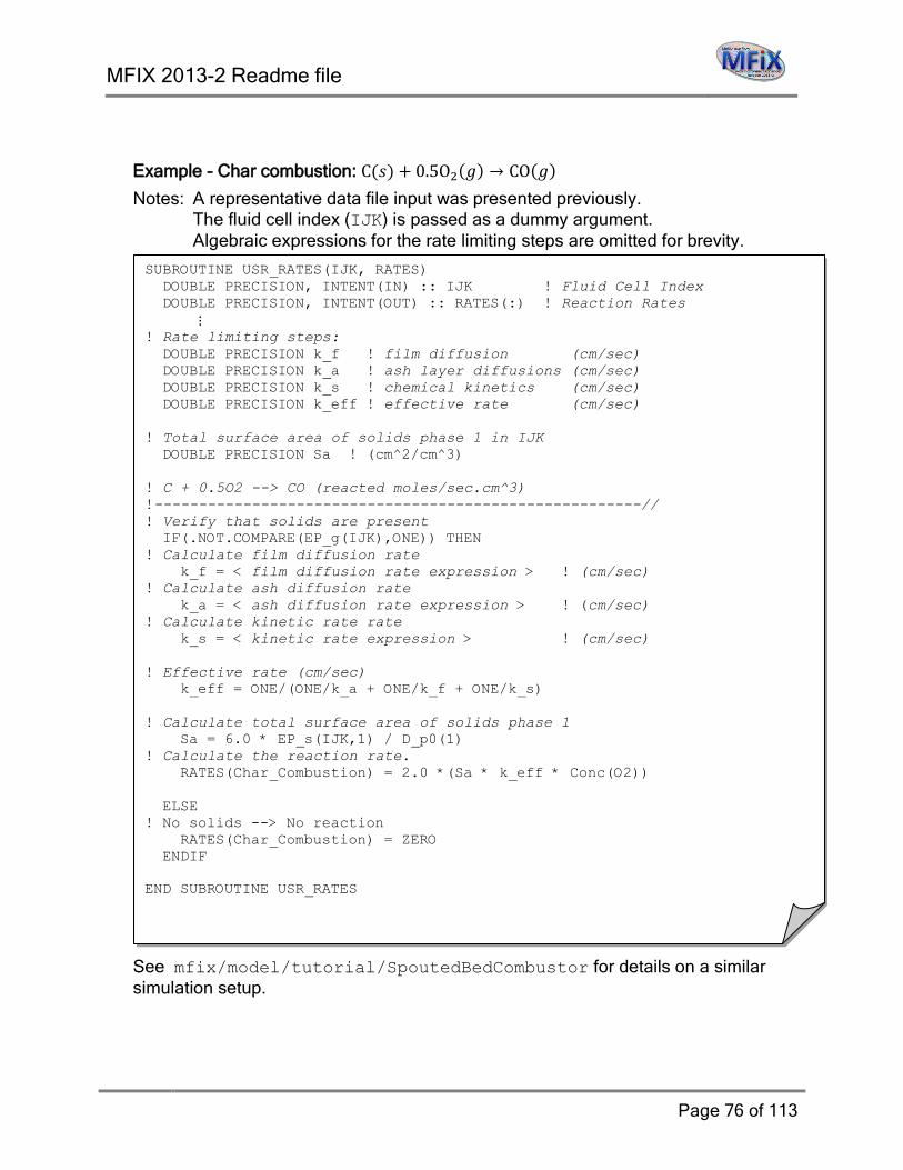
MFIX 2013-2 Readme file
Page 76 of 113
Example - Char combustion: C(𝑠) + 0.5O2(𝑔) → CO(𝑔)
Notes: A representative data file input was presented previously. The fluid cell index (IJK) is passed as a dummy argument. Algebraic expressions for the rate limiting steps are omitted for brevity.
See mfix/model/tutorial/SpoutedBedCombustor for details on a similar simulation setup.
SUBROUTINE USR_RATES(IJK, RATES) DOUBLE PRECISION, INTENT(IN) :: IJK ! Fluid Cell Index DOUBLE PRECISION, INTENT(OUT) :: RATES(:) ! Reaction Rates ⋮ ! Rate limiting steps: DOUBLE PRECISION k_f ! film diffusion (cm/sec) DOUBLE PRECISION k_a ! ash layer diffusions (cm/sec) DOUBLE PRECISION k_s ! chemical kinetics (cm/sec) DOUBLE PRECISION k_eff ! effective rate (cm/sec) ! Total surface area of solids phase 1 in IJK DOUBLE PRECISION Sa ! (cm^2/cm^3) ! C + 0.5O2 --> CO (reacted moles/sec.cm^3) !-------------------------------------------------------// ! Verify that solids are present IF(.NOT.COMPARE(EP_g(IJK),ONE)) THEN ! Calculate film diffusion rate k_f = < film diffusion rate expression > ! (cm/sec) ! Calculate ash diffusion rate k_a = < ash diffusion rate expression > ! (cm/sec) ! Calculate kinetic rate rate k_s = < kinetic rate expression > ! (cm/sec) ! Effective rate (cm/sec) k_eff = ONE/(ONE/k_a + ONE/k_f + ONE/k_s) ! Calculate total surface area of solids phase 1 Sa = 6.0 * EP_s(IJK,1) / D_p0(1) ! Calculate the reaction rate. RATES(Char_Combustion) = 2.0 *(Sa * k_eff * Conc(O2)) ELSE ! No solids --> No reaction RATES(Char_Combustion) = ZERO ENDIF END SUBROUTINE USR_RATES
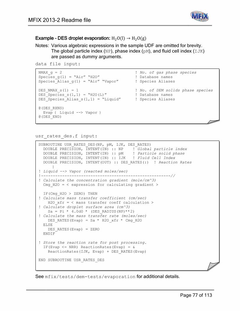
MFIX 2013-2 Readme file
Page 77 of 113
Example – DES droplet evaporation: H2O(l) → H2O(g)
Notes: Various algebraic expressions in the sample UDF are omitted for brevity. The global particle index (NP), phase index (pM), and fluid cell index (IJK) are passed as dummy arguments.
data file input:
usr_rates_des.f input:
See mfix/tests/dem-tests/evaporation for additional details.
SUBROUTINE USR_RATES_DES(NP, pM, IJK, DES_RATES) DOUBLE PRECISION, INTENT(IN) :: NP ! Global particle index DOUBLE PRECISION, INTENT(IN) :: pM ! Particle solid phase DOUBLE PRECISION, INTENT(IN) :: IJK ! Fluid Cell Index DOUBLE PRECISION, INTENT(OUT) :: DES_RATES(:) ! Reaction Rates ⋮ ! Liquid --> Vapor (reacted moles/sec) !-------------------------------------------------------// ! Calculate the concentration gradient (mole/cm^3) Cmg_H2O = < expression for calculating gradient > IF(Cmg_H2O > ZERO) THEN ! Calculate mass transfer coefficient (cm/sec) H2O_xfr = < mass transfer coeff calculation > ! Calculate droplet surface area (cm^3) Sa = Pi * 4.0d0 * (DES_RADIUS(NP)**2) ! Calculate the mass transfer rate (moles/sec) DES_RATES(Evap) = Sa * H2O_xfr * Cmg_H2O ELSE DES_RATES(Evap) = ZERO ENDIF ! Store the reaction rate for post processing. IF(Evap <= NRR) ReactionRates(Evap) = & ReactionRates(IJK, Evap) + DES_RATES(Evap) END SUBROUTINE USR_RATES_DES
NMAX_g = 2 ! No. of gas phase species Species_g(1) = “Air” “H2O” ! Database names Species_Alias_g(1) = “Air” “Vapor” ! Species Aliases DES_NMAX_s(1) = 1 ! No. of DEM solids phase species DES_Species_s(1,1) = “H2O(L)” ! Database names DES_Species_Alias_s(1,1) = “Liquid” ! Species Aliases @(DES_RXNS) Evap { Liquid --> Vapor } @(DES_END)

MFIX 2013-2 Readme file
Page 78 of 113
5. Use make_mfix to (re)build the MFiX executable.
Detailed instructions on building the MFiX executable are given in Section 2.3.1. make_mfix should be ran to update the mfix.exe executable if any one of the following modifications is made:
• the number, order, or alias of any species is changed in the data file.
• the number, order, or name of any chemical reaction is changed in the data file .
• any change is made to chemical reaction rates in either usr_rates.f or usr_rates_des.f.
Additional reaction information::
To write out reaction rates to SPx file:
1. In the data file, mfix.dat, set NRR to the desired number of reaction rates to be written out to the file *.SPA. This number is typically less than or equal to the total number of reactions.
2. In a reaction UDF (usr_rates.f or usr_rates_des.f) assign the desired reaction information to the variable ReactionRates. ReactionRates is a two-dimensional array. The first index references the fluid cell, IJK, while the second index ranges from 1 to NRR.
Two of the above examples illustrate using the ReactionRates variable:
1. Methane Combustion: The calculated reaction rate is directly stored, and logical check is used to prevent over indexing the ReactionRates array.
2. DES droplet evaporation: The calculated reaction rate is added to the storage array. Adding the calculated data to the storage variable is needed in DES since several discrete particles may exist in a single fluid cell. Again, a logical check is preformed to prevent over indexing the array.
If the second index exceeds NRR, a run time error can result from over indexing the array. Using logical checks can eliminate potential errors!
make_mfix preprocesses the data file to generated the species.inc file which is included within the user_rates.f and usr_rates_des.f files as code. Therefore changes in the data file may result in the executable being out of date.

MFIX 2013-2 Readme file
Page 79 of 113
Using an existing (legacy) rrates.f file:
The legacy rrates.f file should be copied to the run directory. Additionally, the following keywords should be specified in the data file:
Keyword (dimension) Type Description
USE_RRATES [.FALSE] L
Use the automated reaction rate UDFS; usr_rates.f and usr_rates_des.f.
.TRUE.
Access legacy rrates.f file for reaction rate information. Rates of formation/consumption as well as heats of reaction are provided by the user.
NMAX(m) [UNDEFINED_I] I
Number of species in phase m. Note that the gas phase is indicated as m=0.
SPECIES_NAME(n)
[UNDEFINED_C]
C
Names of gas and solids phase species as it appears in the materials database. The first NMAX(0) are the names of gas species. The next NMAX(1) are the names of solids phase-1 species, etc.
Additional remarks:
• make_mfix requires that the data file, mfix.dat, be present in the run directory as the species aliases and reaction identifiers are needed to construct a species.inc file.
• Species aliases and reaction identifiers must be unique. make_mfix performs a cursory check on the supplied data and exits if non unique entries are identified.
• If any species alias or reaction identifier conflicts with an existing global variable in MFiX, an error will be reported and the code will fail to compile.
The only modification needed for a legacy mfix.dat and rrates.f file combination is the inclusion of USE_RRATS=.TRUE. in the data file.
An example of legacy file usage: mfix/tutorials/reactor1b
Legacy species keywords , NMAX(m) and SPECIES_NAME(n), are required when using a legacy rrates.f file. Current species keywords NMAX_g, NMAX_s, SPECIES_g, and SPECIES_s cannot be used.
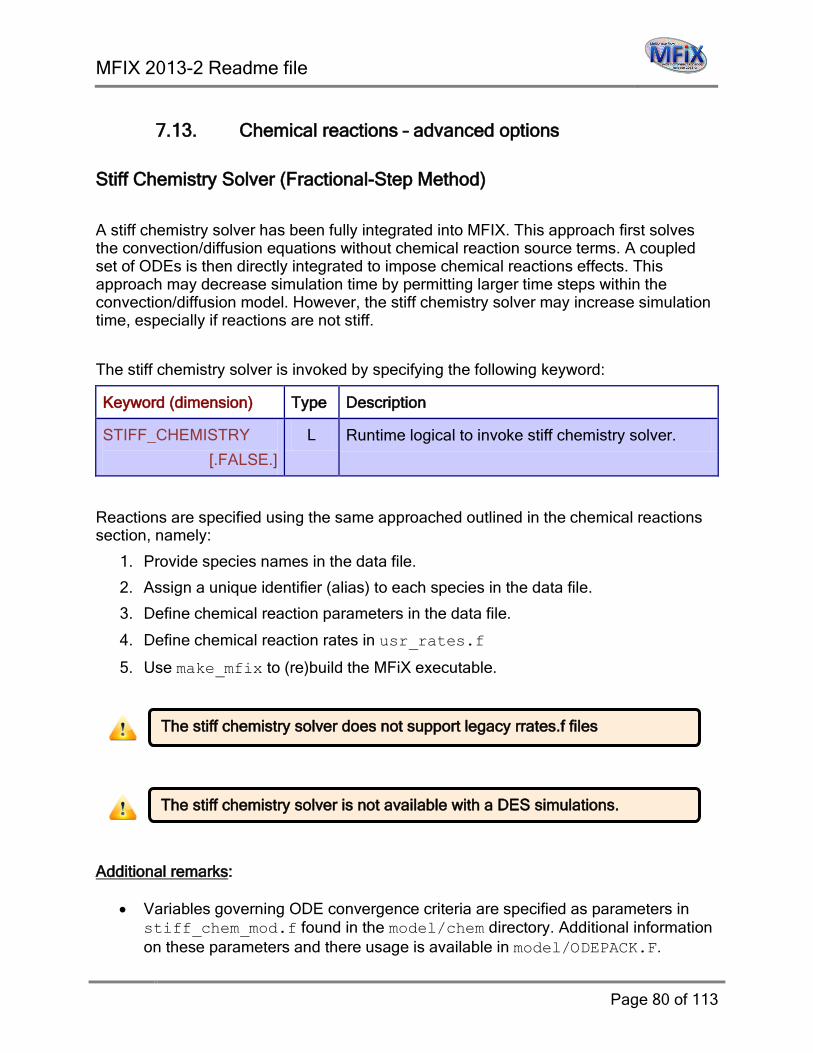
MFIX 2013-2 Readme file
Page 80 of 113
7.13. Chemical reactions – advanced options
Stiff Chemistry Solver (Fractional-Step Method)
A stiff chemistry solver has been fully integrated into MFIX. This approach first solves the convection/diffusion equations without chemical reaction source terms. A coupled set of ODEs is then directly integrated to impose chemical reactions effects. This approach may decrease simulation time by permitting larger time steps within the convection/diffusion model. However, the stiff chemistry solver may increase simulation time, especially if reactions are not stiff.
The stiff chemistry solver is invoked by specifying the following keyword:
Keyword (dimension) Type Description
STIFF_CHEMISTRY
[.FALSE.]
L Runtime logical to invoke stiff chemistry solver.
Reactions are specified using the same approached outlined in the chemical reactions section, namely:
1. Provide species names in the data file.
2. Assign a unique identifier (alias) to each species in the data file.
3. Define chemical reaction parameters in the data file.
4. Define chemical reaction rates in usr_rates.f
5. Use make_mfix to (re)build the MFiX executable.
Additional remarks:
• Variables governing ODE convergence criteria are specified as parameters in stiff_chem_mod.f found in the model/chem directory. Additional information on these parameters and there usage is available in model/ODEPACK.F.
The stiff chemistry solver is not available with a DES simulations.
The stiff chemistry solver does not support legacy rrates.f files

MFIX 2013-2 Readme file
Page 81 of 113
• It is recommend to first run your simulation in debug mode. This will catch some common programmatic errors in the usr_rates.f file. Additionally, the stiff chemistry solver checks for NaNs calculated in the usr_rates.f file.
• The tutorial located in mfix/tutorials/silane_pyrolysis shows how to use the stiff chemistry solver.
ISAT and Direct Integration for Chemical Reactions
MFIX no longer supports implementing reactive chemistry via ISAT (In Situ Adaptive Tabulation). The following keywords are disabled and result in runtime errors when included:
Keyword (dimension) Type Description
CALL_DI L DISABLED
Variable to decide if chemical reactions are time-split and solved using direct integration (DI) with ODE solver.
CALL_ISAT L DISABLED
Variable to decide if chemical reactions are time-split and solved using ISAT.
CALL_GROW L DISABLED
Variable to decide if particle growth due to chemical reactions is calculated.
ISATdt DP DISABLED
Time step for ISAT simulations.

MFIX 2013-2 Readme file
Page 82 of 113
7.14. Thermochemical Properties
The directory mfix/model/thermochemical contains the database of Burcat and Ruscic (2005) and routines for reading the database. With linkage to this database the users need not manually enter data for molecular weight, specific heat, and heats of reactions. Instead the users need to enter the names of the species (keyword SPECIES_g and SPECIES_s) in the data file. MFIX reads the necessary thermo-chemical data from files in the following order:
1. mfix.dat 2. BURCAT.THR file in the run directory 3. mfix/model/thermochemical/BURCAT.THR.
The species names are case sensitive and should match the names in BURCAT.THR exactly; alternatively aliases can be defined for common species, such as O2, in read_therm.f. See mfix/tests/thermo for a sample case that accesses the database. The format of BURCAT.THR file resembles CHEMKIN format, but with several notable differences. Thermochemical data must start below a line that starts with THERMO DATA.
Example dataset from BURCAT.THR with notations:
Each entry in the database starts with a unique CAS identifier (74-82-8) for the species, followed by several lines of comments highlighted in green. The data section starts with the species name in columns 1-18 (CH4 RRHO). Common species names may be followed by strings (RRHO) that identify the method used to determine the coefficients. Additional information follows the species name. The numbers toward the end of the line are the temperature limits (200.000 6000.000) in degrees Kelvin where the property calculation is valid and the molecular weight (16.04246). Unlike CHEMKIN the common temperature for the high and low temperature branches are not recorded; it is always 1000 K. The next three lines give the fourteen coefficients (seven
1.91178600E+00 9.60267960E-03 -3.38387841E-06 5.38797240E-10 -3.19306807E-14
-1.00992136E+04 8.48241861E+00 5.14825732E+00 -1.37002410E-02 4.93749414E-05 -4.91952339E-08 1.70097299E-11 -1.02453222E+04 -4.63322726E+00 -8.97226656E+03
CH4 RRHO g 8/99C 1.H 4. 0. 0.G 200.000 6000.000 B 16.04246 1
than the NRRAO2. Max Lst Sq Error Cp @ 6000. K 0.62%.
3
4
CH4 METHANE Same as the Anharmonic but calculated Using the RRHO method rather
74-82-8
2
CAS identifier
valid temperature
range
molecular weight
comments
formation enthalpy at
298K
species name
high temperature coefficients
low temperature coefficients
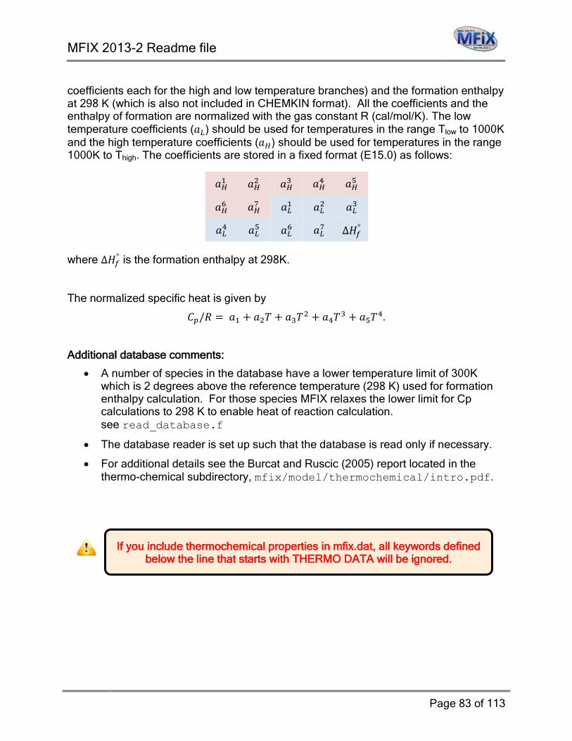
MFIX 2013-2 Readme file
Page 83 of 113
coefficients each for the high and low temperature branches) and the formation enthalpy at 298 K (which is also not included in CHEMKIN format). All the coefficients and the enthalpy of formation are normalized with the gas constant R (cal/mol/K). The low temperature coefficients (𝑎𝐿) should be used for temperatures in the range Tlow to 1000K and the high temperature coefficients (𝑎𝐻) should be used for temperatures in the range 1000K to Thigh. The coefficients are stored in a fixed format (E15.0) as follows:
where Δ𝐻𝑓° is the formation enthalpy at 298K.
The normalized specific heat is given by
𝐶𝑝/𝑅 = 𝑎1 + 𝑎2𝑇 + 𝑎3𝑇2 + 𝑎4𝑇3 + 𝑎5𝑇4.
Additional database comments:
• A number of species in the database have a lower temperature limit of 300K which is 2 degrees above the reference temperature (298 K) used for formation enthalpy calculation. For those species MFIX relaxes the lower limit for Cp calculations to 298 K to enable heat of reaction calculation. see read_database.f
• The database reader is set up such that the database is read only if necessary.
• For additional details see the Burcat and Ruscic (2005) report located in the thermo-chemical subdirectory, mfix/model/thermochemical/intro.pdf.
If you include thermochemical properties in mfix.dat, all keywords defined below the line that starts with THERMO DATA will be ignored.
𝑎𝐻1 𝑎𝐻2 𝑎𝐻3 𝑎𝐻4 𝑎𝐻5
𝑎𝐻6 𝑎𝐻7 𝑎𝐿1 𝑎𝐿2 𝑎𝐿3
Δ𝐻𝑓° 𝑎𝐿7 𝑎𝐿6 𝑎𝐿5 𝑎𝐿4
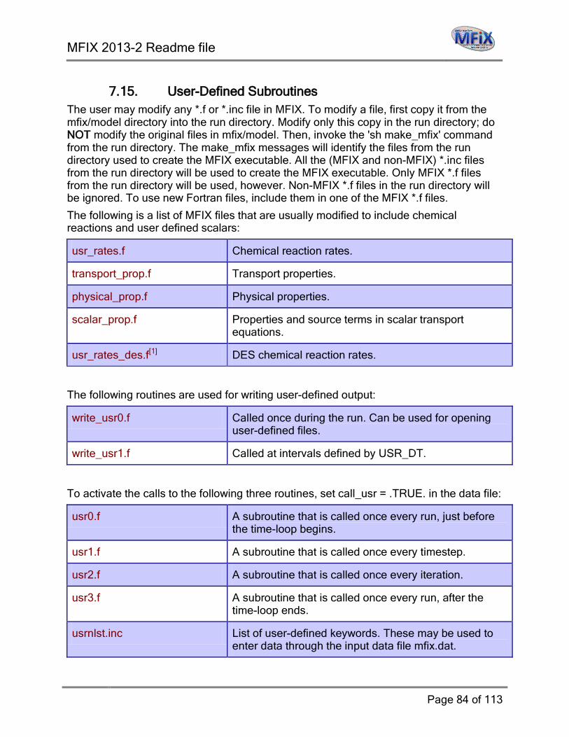
MFIX 2013-2 Readme file
Page 84 of 113
7.15. User-Defined Subroutines The user may modify any *.f or *.inc file in MFIX. To modify a file, first copy it from the mfix/model directory into the run directory. Modify only this copy in the run directory; do NOT modify the original files in mfix/model. Then, invoke the 'sh make_mfix' command from the run directory. The make_mfix messages will identify the files from the run directory used to create the MFIX executable. All the (MFIX and non-MFIX) *.inc files from the run directory will be used to create the MFIX executable. Only MFIX *.f files from the run directory will be used, however. Non-MFIX *.f files in the run directory will be ignored. To use new Fortran files, include them in one of the MFIX *.f files.
The following is a list of MFIX files that are usually modified to include chemical reactions and user defined scalars:
usr_rates.f Chemical reaction rates.
transport_prop.f Transport properties.
physical_prop.f Physical properties.
scalar_prop.f Properties and source terms in scalar transport equations.
usr_rates_des.f[1] DES chemical reaction rates.
The following routines are used for writing user-defined output:
write_usr0.f Called once during the run. Can be used for opening user-defined files.
write_usr1.f Called at intervals defined by USR_DT.
To activate the calls to the following three routines, set call_usr = .TRUE. in the data file:
usr0.f A subroutine that is called once every run, just before the time-loop begins.
usr1.f A subroutine that is called once every timestep.
usr2.f A subroutine that is called once every iteration.
usr3.f A subroutine that is called once every run, after the time-loop ends.
usrnlst.inc List of user-defined keywords. These may be used to enter data through the input data file mfix.dat.
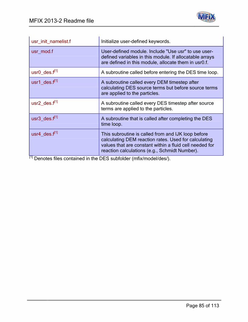
MFIX 2013-2 Readme file
Page 85 of 113
usr_init_namelist.f Initialize user-defined keywords.
usr_mod.f User-defined module. Include "Use usr" to use user-defined variables in this module. If allocatable arrays are defined in this module, allocate them in usr0.f.
usr0_des.f[1] A subroutine called before entering the DES time loop.
usr1_des.f[1] A subroutine called every DEM timestep after calculating DES source terms but before source terms are applied to the particles.
usr2_des.f[1] A subroutine called every DES timestep after source terms are applied to the particles.
usr3_des.f[1] A subroutine that is called after completing the DES time loop.
usr4_des.f[1] This subroutine is called from and IJK loop before calculating DEM reaction rates. Used for calculating values that are constant within a fluid cell needed for reaction calculations (e.g., Schmidt Number).
[1] Denotes files contained in the DES subfolder (mfix/model/des/).

MFIX 2013-2 Readme file
Page 86 of 113
DES User-defined subroutine call structure:
calculate DES hydrodynamic and
energy source terms
call to user1_des.f
update DES variables
call to user2_des.f
reacting flow
calculate DES reaction source terms
Loop over fluid cells (IJK)
call to user4_des.f
loop over particles in fluid cell IJK
call to user_rates_des.f
no
yes
DES Time Loop
Pass off from continuum phase
model
call to user0_des.f
Pass off to continuum phase
model
call to user3_des.f

MFIX 2013-2 Readme file
Page 87 of 113
7.16. Parallelization Controls
Keyword (dimension) Type Description
NODESI
[1]
I Number of grid blocks in x-direction.
NODESJ
[1]
I Number of grid blocks in y-direction.
NODESK
[1]
I Number of grid blocks in z-direction.
MINIMIZE_DOTPRODUCTS
[.FALSE.]
L The dot products calculations in BiCGStab are minimized and this should only have impact on parallel runs
SOLVER_STATISTICS
[.FALSE.]
L Print out additional statistics for parallel runs
DEBUG_RESID
[.TRUE.]
L If set to false, the residuals are grouped into far fewer global collectives and this should only have impact on parallel runs
NODESI * NODESJ * NODESK must be the same as the number of processors specified using the mpirun (or equivalent command). Otherwise the code will return with an error.
The parallel performance depends on several things and one has to evaluate different options before choosing the right strategy for the problem at hand. For e.g. if the J direction is the strongest coupled direction, the preconditioning for the linear solver will be poor if there is decomposition in that direction. However, since decomposing in all the directions reduces the processor grid surface area to the volume, the communication cost will be less for the same computational grid. The preconditioners are chosen with the keyword LEQ_PC. In addition to LINE relaxation, one can choose the “DIAG” or “NONE” preconditioners that reduces interprocessor communications but would increase the number of linear equation solver iterations. The DIAG and NONE choices for preconditioners may be appropriate for all equations except the continuity (or pressure and volume fraction correction) equations. The parallel performance is greatly dependent on the choices stated here, and some trial an error may be required to determine the right combination of decomposition direction and the choice of preconditioners to get the best performance in production runs.
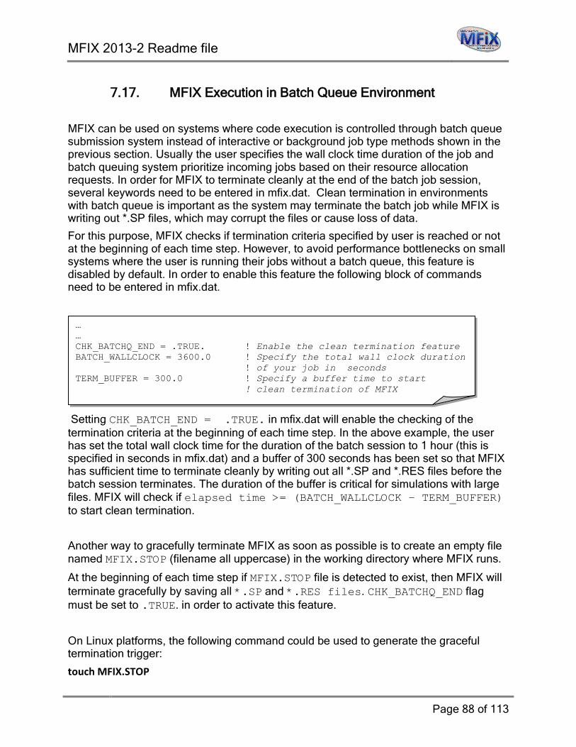
MFIX 2013-2 Readme file
Page 88 of 113
7.17. MFIX Execution in Batch Queue Environment
MFIX can be used on systems where code execution is controlled through batch queue submission system instead of interactive or background job type methods shown in the previous section. Usually the user specifies the wall clock time duration of the job and batch queuing system prioritize incoming jobs based on their resource allocation requests. In order for MFIX to terminate cleanly at the end of the batch job session, several keywords need to be entered in mfix.dat. Clean termination in environments with batch queue is important as the system may terminate the batch job while MFIX is writing out *.SP files, which may corrupt the files or cause loss of data.
For this purpose, MFIX checks if termination criteria specified by user is reached or not at the beginning of each time step. However, to avoid performance bottlenecks on small systems where the user is running their jobs without a batch queue, this feature is disabled by default. In order to enable this feature the following block of commands need to be entered in mfix.dat.
Setting CHK_BATCH_END = .TRUE. in mfix.dat will enable the checking of the termination criteria at the beginning of each time step. In the above example, the user has set the total wall clock time for the duration of the batch session to 1 hour (this is specified in seconds in mfix.dat) and a buffer of 300 seconds has been set so that MFIX has sufficient time to terminate cleanly by writing out all *.SP and *.RES files before the batch session terminates. The duration of the buffer is critical for simulations with large files. MFIX will check if elapsed time >= (BATCH_WALLCLOCK – TERM_BUFFER) to start clean termination.
Another way to gracefully terminate MFIX as soon as possible is to create an empty file named MFIX.STOP (filename all uppercase) in the working directory where MFIX runs.
At the beginning of each time step if MFIX.STOP file is detected to exist, then MFIX will terminate gracefully by saving all *.SP and *.RES files. CHK_BATCHQ_END flag must be set to .TRUE. in order to activate this feature.
On Linux platforms, the following command could be used to generate the graceful termination trigger:
touch MFIX.STOP
… … CHK_BATCHQ_END = .TRUE. ! Enable the clean termination feature BATCH_WALLCLOCK = 3600.0 ! Specify the total wall clock duration ! of your job in seconds TERM_BUFFER = 300.0 ! Specify a buffer time to start ! clean termination of MFIX

MFIX 2013-2 Readme file
Page 89 of 113
DO NOT forget to erase the file once MFIX terminates, otherwise next time you run MFIX in the same directory it will terminate immediately.
rm -f -r ./MFIX.STOP
Keyword (dimension) Type Description
CHK_BATCHQ_END
[.FALSE.]
L Enables clean termination feature.
BATCH_WALLCLOCK
[9000.0]
DP Total wall-clock duration of the job, in seconds.
TERM_BUFFER
[180.0]
DP Buffer time when initiating clean termination, in seconds.
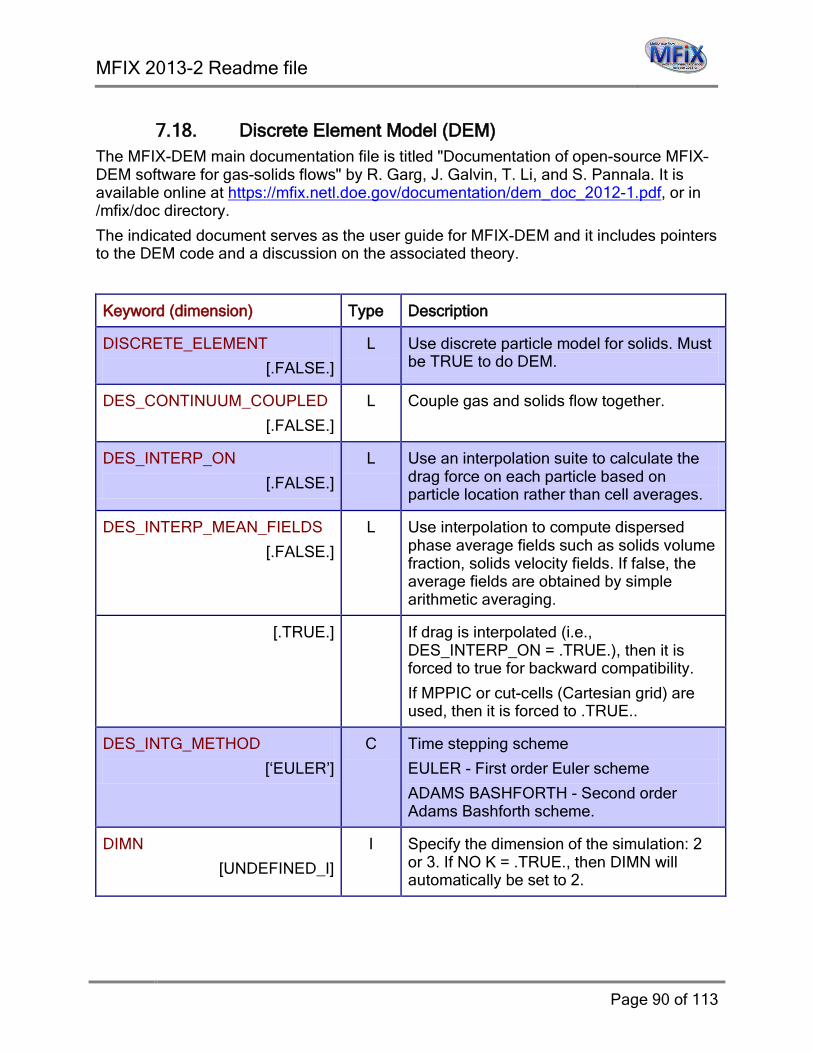
MFIX 2013-2 Readme file
Page 90 of 113
7.18. Discrete Element Model (DEM) The MFIX-DEM main documentation file is titled "Documentation of open-source MFIX–DEM software for gas-solids flows" by R. Garg, J. Galvin, T. Li, and S. Pannala. It is available online at https://mfix.netl.doe.gov/documentation/dem_doc_2012-1.pdf, or in /mfix/doc directory.
The indicated document serves as the user guide for MFIX-DEM and it includes pointers to the DEM code and a discussion on the associated theory.
Keyword (dimension) Type Description
DISCRETE_ELEMENT
[.FALSE.]
L Use discrete particle model for solids. Must be TRUE to do DEM.
DES_CONTINUUM_COUPLED
[.FALSE.]
L Couple gas and solids flow together.
DES_INTERP_ON
[.FALSE.]
L Use an interpolation suite to calculate the drag force on each particle based on particle location rather than cell averages.
DES_INTERP_MEAN_FIELDS
[.FALSE.]
L Use interpolation to compute dispersed phase average fields such as solids volume fraction, solids velocity fields. If false, the average fields are obtained by simple arithmetic averaging.
[.TRUE.] If drag is interpolated (i.e., DES_INTERP_ON = .TRUE.), then it is forced to true for backward compatibility.
If MPPIC or cut-cells (Cartesian grid) are used, then it is forced to .TRUE..
DES_INTG_METHOD
[‘EULER’]
C Time stepping scheme
EULER - First order Euler scheme
ADAMS BASHFORTH - Second order Adams Bashforth scheme.
DIMN
[UNDEFINED_I]
I Specify the dimension of the simulation: 2 or 3. If NO K = .TRUE., then DIMN will automatically be set to 2.

MFIX 2013-2 Readme file
Page 91 of 113
GENER_PART_CONFIG
[.FALSE.]
L Automatically generate an initial particle configuration (position) otherwise use particle input.dat. Also requires setting VOL_FRAC(M), D_P0(M), and DES_EPS_XSTART, DES_EPS_YSTART , and DES_EPS_ZSTART. Once defined this feature will determine the total number of particles in the system and their initial placement. The particle input.dat file is ignored.
VOL_FRAC(M)
[UNDEFINED]
DP Only relevant when GENER_PART_CONFIG is T. Volume fraction of the solid phase M for generating articles in the specified domain.
DES_EPS_XSTART
[UNDEFINED]
DP Only needed if GENER_PART_CONFIG. Length of the domain in the x direction wherein particles may be initially placed.
DES_EPS_YSTART
[UNDEFINED]
DP Only needed if GENER_PART_CONFIG. Length of the domain in the y direction wherein particles may be initially placed.
DES_EPS_ZSTART
[UNDEFINED]
DP Only needed if GENER_PART_CONFIG. Length of the domain in the z direction wherein particles may be initially placed.
NFACTOR
[10.0]
I Only needed if DES_CONTINUUM_COUPLED. Number of times a pure DEM simulation is run before the coupled DEM simulation is started (allows settling).
TSUJI_DRAG
[.FALSE.]
L Use Tsuji’s drag correlation. This correlation is only relevant when invoking Syamlal and O'Brien drag model.
PARTICLES
[UNDEFINED_I]
I Total number of particles.
PARTICLES_FACTOR
[1.2]
DP Expand the size of the particle arrays by an arbitrary factor (multiple of the number of particles).

MFIX 2013-2 Readme file
Page 92 of 113
PVEL_MEAN
[0.0]
DP Assign initial particle velocities from a Gaussian distribution with the specified mean. Only relevant if PVEL_STDEV is not zero. If used, the assigned velocities will override any other initial settings.
PVEL_STDEV
[0.0]
DP If not zero, then assign initial particle velocities from a Gaussian distribution with the specified standard deviation. Used with PVEL_MEAN. If used, the assigned velocities will override any other initial settings.
Boundary Conditions Related Keywords for DEM
Keyword (dimension) Type Description
WALLDTSPLIT
[.FALSE.]
L Treat wall interaction as a two-particle interaction but accounting for the wall properties. Must be TRUE for DEM.
DES_PERIODIC_WALLS
[.FALSE.]
L Periodic wall boundary condition is imposed on any pair of walls.
DES_PERIODIC_WALLS_X
[.FALSE.]
L Direction of periodicity: X.
DES_PERIODIC_WALLS_Y
[.FALSE.]
L Direction of periodicity: Y.
DES_PERIODIC_WALLS_Z
[.FALSE.]
L Direction of periodicity: Z.

MFIX 2013-2 Readme file
Page 93 of 113
DES Neighbor Search Related flags needed in DEM model
Keyword (dimension) Type Description
DES_NEIGHBOR_SEARCH
[1]
I Neighbor search algorithm. 1=N-square; 2=quadtree (for 2D only); 3=octree (for 3D only); 4=grid based. Options 2 and 3 have not been recently tested. Use them at your own risk.
NEIGHBOR_SEARCH_N
[25]
I Maximum number of steps through a DEM loop before a neighbor search will be performed. (Search may be called earlier).
MN
[10]
I Maximum number of neighbors per particle.
QLM
[1]
I Number of levels to traverse “up” to move a particle to its new quad. Only needed when using octree or quadtree based neighbor search.
QLN
[1]
I Number of levels to traverse “up” to perform particle neighbor search. Only needed when using octree or quadtree based neighbor search.
INIT_QUAD_COUNT
[UNDEFINED I]
I Count to initialize quadtree or octree. Only needed when using octree or quadtree based neighbor search.
MQUAD_FACTOR
[1.1]
DP Factor to create quadtree or octree arrays based on the number of particles. Only needed when using octree or quadtree based neighbor search.
NEIGHBOR_SEARCH_RAD_RATIO
[1.0]
DP Ratio of the distance (imaginary sphere radius) to particle radius that is allowed before a neighbor search is performed.
FACTOR_RLM
[1.2]
DP Effectively increase the radius of a particle (multiple of the sum of particle radii) for detecting neighbor contacts when using grid based neighbor search or n-square search methods.
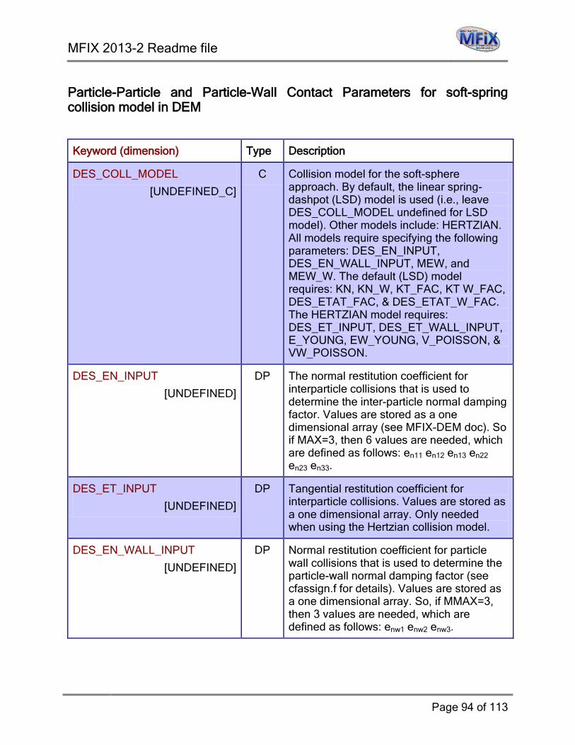
MFIX 2013-2 Readme file
Page 94 of 113
Particle-Particle and Particle-Wall Contact Parameters for soft-spring collision model in DEM
Keyword (dimension) Type Description
DES_COLL_MODEL
[UNDEFINED_C]
C Collision model for the soft-sphere approach. By default, the linear spring-dashpot (LSD) model is used (i.e., leave DES_COLL_MODEL undefined for LSD model). Other models include: HERTZIAN. All models require specifying the following parameters: DES_EN_INPUT, DES_EN_WALL_INPUT, MEW, and MEW_W. The default (LSD) model requires: KN, KN_W, KT_FAC, KT W_FAC, DES_ETAT_FAC, & DES_ETAT_W_FAC. The HERTZIAN model requires: DES_ET_INPUT, DES_ET_WALL_INPUT, E_YOUNG, EW_YOUNG, V_POISSON, & VW_POISSON.
DES_EN_INPUT
[UNDEFINED]
DP The normal restitution coefficient for interparticle collisions that is used to determine the inter-particle normal damping factor. Values are stored as a one dimensional array (see MFIX-DEM doc). So if MAX=3, then 6 values are needed, which are defined as follows: en11 en12 en13 en22 en23 en33.
DES_ET_INPUT
[UNDEFINED]
DP Tangential restitution coefficient for interparticle collisions. Values are stored as a one dimensional array. Only needed when using the Hertzian collision model.
DES_EN_WALL_INPUT
[UNDEFINED]
DP Normal restitution coefficient for particle wall collisions that is used to determine the particle-wall normal damping factor (see cfassign.f for details). Values are stored as a one dimensional array. So, if MMAX=3, then 3 values are needed, which are defined as follows: enw1 enw2 enw3.

MFIX 2013-2 Readme file
Page 95 of 113
DES_ET_WALL_INPUT
[UNDEFINED]
DP Tangential restitution coefficient for particle wall collisions. Values are stored as a one dimensional array. Only needed when using the Hertzian collision model.
KN
[UNDEFINED]
DP Normal spring constant for inter-particle collisions. Values are stored as a one dimensional array. Needed when using the default (LSD) collision model.
KT_FAC
[2/7]
DP Ratio of the tangential spring constant to normal spring constant for inter-particle collisions. Use it to specify the tangential spring constant for particle-particle collisions as KT_FAC*KN. Needed when using the default (LSD) collision model.
DES_ETAT_FAC
[0.5]
DP Ratio of the tangential damping factor to the normal damping factor for inter-particle collisions. Needed when using the default (LSD) collision model.
KN_W
[UNDEFINED]
DP Normal spring constant for particle-wall collisions. Needed when using the default (LSD) collision model.
KT_W_FAC
[2/7]
DP Ratio of the tangential spring constant to normal spring constant for particle-wall collisions. Use it to specify the tangential spring constant for particle-wall collisions as KT_W_FAC*KN_W. Needed when using the default (LSD) collision model.
DES_ETAT_W_FAC
[0.5]
DP Ratio of the tangential damping factor to the normal damping factor for particle wall collisions. Needed when using the default (LSD) collision model.
MEW
[UNDEFINED]
DP Particle friction coefficient.
MEW_W
[UNDEFINED]
DP Particle-wall friction coefficient.
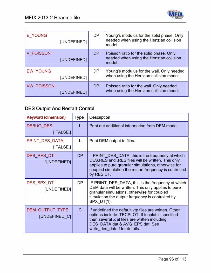
MFIX 2013-2 Readme file
Page 96 of 113
E_YOUNG
[UNDEFINED]
DP Young’s modulus for the solid phase. Only needed when using the Hertzian collision model.
V_POISSON
[UNDEFINED]
DP Poisson ratio for the solid phase. Only needed when using the Hertzian collision model.
EW_YOUNG
[UNDEFINED]
DP Young’s modulus for the wall. Only needed when using the Hertzian collision model.
VW_POISSON
[UNDEFINED]
DP Poisson ratio for the wall. Only needed when using the Hertzian collision model.
DES Output And Restart Control
Keyword (dimension) Type Description
DEBUG_DES
[.FALSE.]
L Print out additional information from DEM model.
PRINT_DES_DATA
[.FALSE.]
L Print DEM output to files.
DES_RES_DT
[UNDEFINED]
DP If PRINT_DES_DATA, this is the frequency at which DES.RES and .RES files will be written. This only applies to pure granular simulations, otherwise for coupled simulation the restart frequency is controlled by RES DT.
DES_SPX_DT
[UNDEFINED]
DP IF PRINT_DES_DATA, this is the frequency at which DEM data will be written. This only applies to pure granular simulations, otherwise for coupled simulation the output frequency is controlled by SPX_DT(1).
DEM_OUTPUT_TYPE
[UNDEFINED_C]
C If undefined the default vtp files are written. Other options include: TECPLOT. If tecplot is specified then several .dat files are written including DES_DATA.dat & AVG_EPS.dat. See write_des_data.f for details.

MFIX 2013-2 Readme file
Page 97 of 113
DEM Mass Inlet/Outlet Specifications: DEM mass inlet or outlet (bc) are specified over flow planes or 2D surfaces that are normal to one of the coordinate directions and coincide with a face of the scalar control-volume. The values for one of the three pairs of coordinates are equal. The surface is defined by the constant coordinates of each of the four edges and the two equal values for the direction normal to the face. These are specified with physical coordinates. A flow plane must have a wall cell (or an outside boundary) on one side and a flow cell on the other side
For a mass inflow boundary the discrete solids flow rates are specified as the volumetric or mass flow rates. The phase-M flow rates are converted to an equivalent number of phase-m discrete particles enter the system. A uniform inlet velocity is then selected that minimizes the error between the specified bulk density values and the calculated bulk density values. For details see Musser et al., “Development of a discrete mass inflow boundary condition for MFIX”, Journal of Systemics, Cybernetics and Informatics (JSCI), Volume 9, Number 1, 2011, pg 94-98. Keyword (dimension) Type Description
MAX_PIS
[UNDEFINED_I]
I Maximum number of particles that may exist within a simulation. This quantity is used for calculating the size of arrays for allocation.
DES_BC_X_w(bc)
[UNDEFINED]
DP x coordinate of the west face
DES_BC_X_e(bc)
[UNDEFINED]
DP x coordinate of the east face
DES_BC_Y_s(bc)
[UNDEFINED]
DP y coordinate of the south face
DES_BC_Y_n(bc)
[UNDEFINED]
DP y coordinate of the north face
DES_BC_Z_b(bc)
[UNDEFINED]
DP z coordinate of the bottom face
DES_BC_Z_t(bc)
[UNDEFINED]
DP z coordinate of the top face
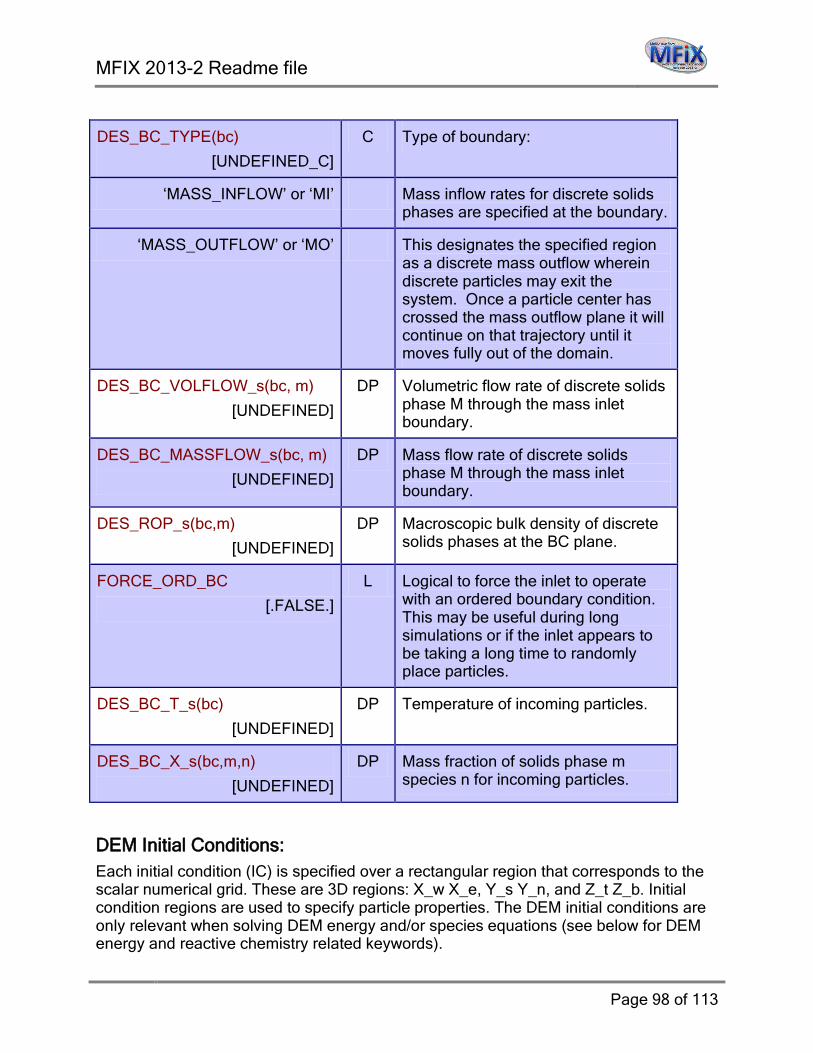
MFIX 2013-2 Readme file
Page 98 of 113
DES_BC_TYPE(bc)
[UNDEFINED_C]
C Type of boundary:
‘MASS_INFLOW’ or ‘MI’ Mass inflow rates for discrete solids phases are specified at the boundary.
‘MASS_OUTFLOW’ or ‘MO’ This designates the specified region as a discrete mass outflow wherein discrete particles may exit the system. Once a particle center has crossed the mass outflow plane it will continue on that trajectory until it moves fully out of the domain.
DES_BC_VOLFLOW_s(bc, m)
[UNDEFINED]
DP Volumetric flow rate of discrete solids phase M through the mass inlet boundary.
DES_BC_MASSFLOW_s(bc, m)
[UNDEFINED]
DP Mass flow rate of discrete solids phase M through the mass inlet boundary.
DES_ROP_s(bc,m)
[UNDEFINED]
DP Macroscopic bulk density of discrete solids phases at the BC plane.
FORCE_ORD_BC
[.FALSE.]
L Logical to force the inlet to operate with an ordered boundary condition. This may be useful during long simulations or if the inlet appears to be taking a long time to randomly place particles.
DES_BC_T_s(bc)
[UNDEFINED]
DP Temperature of incoming particles.
DES_BC_X_s(bc,m,n)
[UNDEFINED]
DP Mass fraction of solids phase m species n for incoming particles.
DEM Initial Conditions: Each initial condition (IC) is specified over a rectangular region that corresponds to the scalar numerical grid. These are 3D regions: X_w X_e, Y_s Y_n, and Z_t Z_b. Initial condition regions are used to specify particle properties. The DEM initial conditions are only relevant when solving DEM energy and/or species equations (see below for DEM energy and reactive chemistry related keywords).

MFIX 2013-2 Readme file
Page 99 of 113
Keyword (dimension) Type Description
DES_IC_X_w(ic)
[UNDEFINED]
DP x coordinate of the west face
DES_IC_X_e(ic)
[UNDEFINED]
DP x coordinate of the east face
DES_IC_Y_s(ic)
[UNDEFINED]
DP y coordinate of the south face
DES_IC_Y_n(ic)
[UNDEFINED]
DP y coordinate of the north face
DES_IC_Z_b(ic)
[UNDEFINED]
DP z coordinate of the bottom face
DES_IC_Z_t(ic)
[UNDEFINED]
DP z coordinate of the top face
DEM Energy Equations:
Keyword (dimension) Type Description
DES_ENERGY_EQ
[.FALSE.]
L Solve energy equations for DEM.
DES_CONV_EQ
[.TRUE.]
L Include particle-gas convection in DEM heat transfer model.
DES_COND_EQ
[.TRUE.]
L Include particle-particle conduction in DEM heat transfer model.
DES_COND_EQ_PP
[.TRUE.]
L Include particle-particle contact conduction in DEM heat transfer model. (Requires DES_COND_EQ set to true.)
DES_COND_EQ_PFP
[.TRUE.]
L Include particle-fluid-particle conduction in DEM heat transfer model. (Requires DES_COND_EQ set to true.)
DES_RADI_EQ L Include particle--particle radiation in DEM heat transfer model.
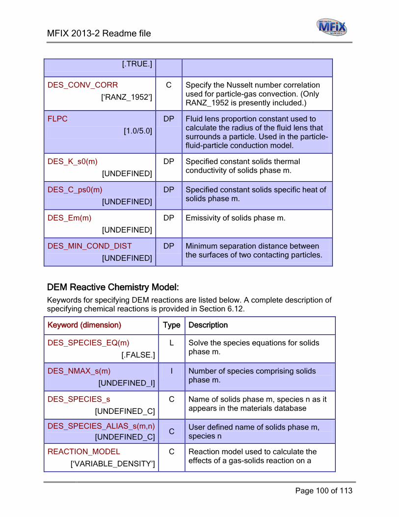
MFIX 2013-2 Readme file
Page 100 of 113
[.TRUE.]
DES_CONV_CORR
[‘RANZ_1952’]
C Specify the Nusselt number correlation used for particle-gas convection. (Only RANZ_1952 is presently included.)
FLPC
[1.0/5.0]
DP Fluid lens proportion constant used to calculate the radius of the fluid lens that surrounds a particle. Used in the particle-fluid-particle conduction model.
DES_K_s0(m)
[UNDEFINED]
DP Specified constant solids thermal conductivity of solids phase m.
DES_C_ps0(m)
[UNDEFINED]
DP Specified constant solids specific heat of solids phase m.
DES_Em(m)
[UNDEFINED]
DP Emissivity of solids phase m.
DES_MIN_COND_DIST
[UNDEFINED]
DP Minimum separation distance between the surfaces of two contacting particles.
DEM Reactive Chemistry Model: Keywords for specifying DEM reactions are listed below. A complete description of specifying chemical reactions is provided in Section 6.12.
Keyword (dimension) Type Description
DES_SPECIES_EQ(m)
[.FALSE.]
L Solve the species equations for solids phase m.
DES_NMAX_s(m)
[UNDEFINED_I]
I Number of species comprising solids phase m.
DES_SPECIES_s
[UNDEFINED_C]
C Name of solids phase m, species n as it appears in the materials database
DES_SPECIES_ALIAS_s(m,n) [UNDEFINED_C]
C User defined name of solids phase m, species n
REACTION_MODEL
[‘VARIABLE_DENSITY’]
C Reaction model used to calculate the effects of a gas-solids reaction on a
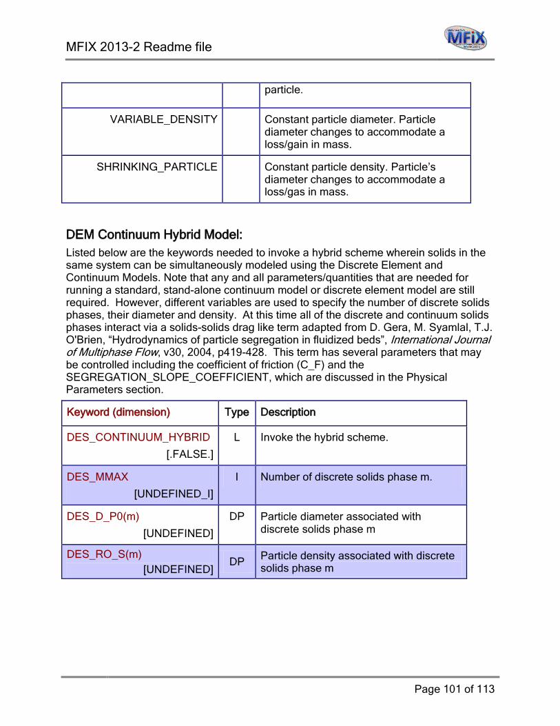
MFIX 2013-2 Readme file
Page 101 of 113
particle.
VARIABLE_DENSITY Constant particle diameter. Particle diameter changes to accommodate a loss/gain in mass.
SHRINKING_PARTICLE Constant particle density. Particle’s diameter changes to accommodate a loss/gas in mass.
DEM Continuum Hybrid Model: Listed below are the keywords needed to invoke a hybrid scheme wherein solids in the same system can be simultaneously modeled using the Discrete Element and Continuum Models. Note that any and all parameters/quantities that are needed for running a standard, stand-alone continuum model or discrete element model are still required. However, different variables are used to specify the number of discrete solids phases, their diameter and density. At this time all of the discrete and continuum solids phases interact via a solids-solids drag like term adapted from D. Gera, M. Syamlal, T.J. O'Brien, “Hydrodynamics of particle segregation in fluidized beds”, International Journal of Multiphase Flow, v30, 2004, p419-428. This term has several parameters that may be controlled including the coefficient of friction (C_F) and the SEGREGATION_SLOPE_COEFFICIENT, which are discussed in the Physical Parameters section.
Keyword (dimension) Type Description
DES_CONTINUUM_HYBRID
[.FALSE.]
L Invoke the hybrid scheme.
DES_MMAX
[UNDEFINED_I]
I Number of discrete solids phase m.
DES_D_P0(m)
[UNDEFINED]
DP Particle diameter associated with discrete solids phase m
DES_RO_S(m) [UNDEFINED]
DP Particle density associated with discrete solids phase m
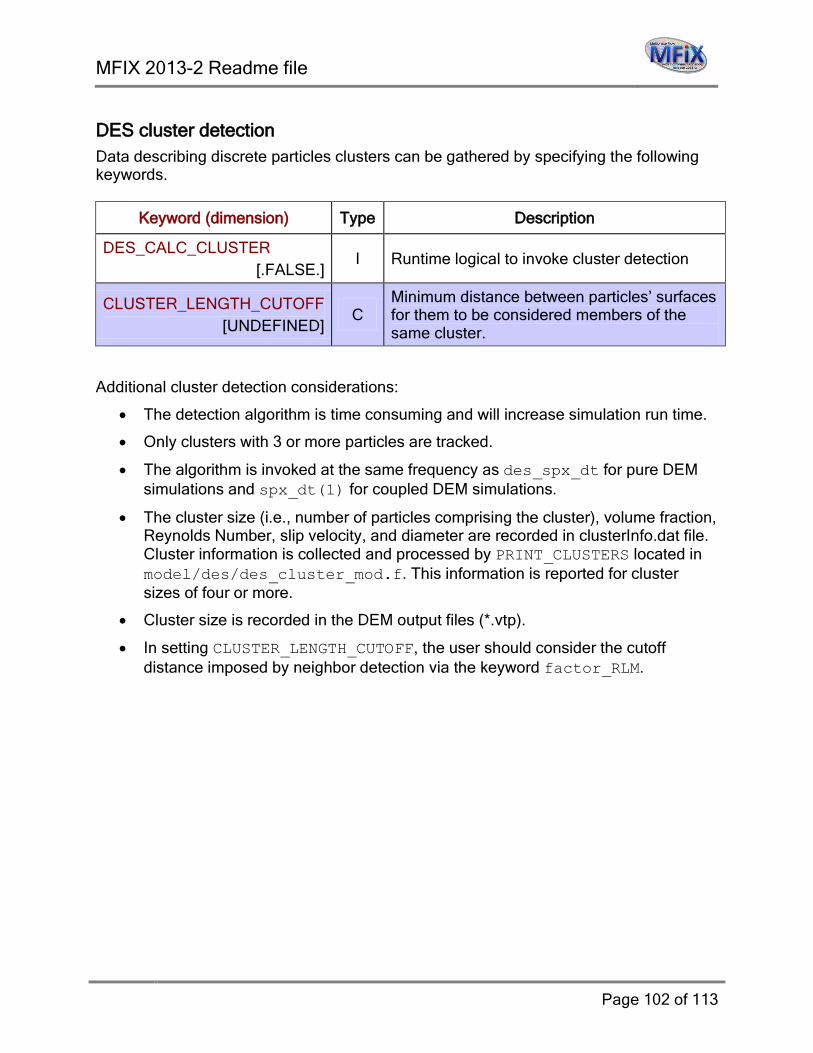
MFIX 2013-2 Readme file
Page 102 of 113
DES cluster detection Data describing discrete particles clusters can be gathered by specifying the following keywords.
Keyword (dimension) Type Description
DES_CALC_CLUSTER [.FALSE.]
I Runtime logical to invoke cluster detection
CLUSTER_LENGTH_CUTOFF [UNDEFINED]
C Minimum distance between particles’ surfaces for them to be considered members of the same cluster.
Additional cluster detection considerations:
• The detection algorithm is time consuming and will increase simulation run time.
• Only clusters with 3 or more particles are tracked.
• The algorithm is invoked at the same frequency as des_spx_dt for pure DEM simulations and spx_dt(1) for coupled DEM simulations.
• The cluster size (i.e., number of particles comprising the cluster), volume fraction, Reynolds Number, slip velocity, and diameter are recorded in clusterInfo.dat file. Cluster information is collected and processed by PRINT_CLUSTERS located in model/des/des_cluster_mod.f. This information is reported for cluster sizes of four or more.
• Cluster size is recorded in the DEM output files (*.vtp).
• In setting CLUSTER_LENGTH_CUTOFF, the user should consider the cutoff distance imposed by neighbor detection via the keyword factor_RLM.

MFIX 2013-2 Readme file
Page 103 of 113
7.19. MPPIC model: The MFIX-DEM main documentation file is titled "Documentation of open-source MFIX–PIC software for gas-solids flows" by R. Garg and J. F. Dietiker. It is available online at https://mfix.netl.doe.gov/documentation/mfix_pic_doc.pdf, or in /mfix/doc directory.
The indicated document serves as the theory guide for the MPPIC model implementation details in MFIX code. The MFIX code with MPPIC model is referred to as MFIX-PIC in the indicated document and hereinafter. A brief discussion on setting up of input file for MPPIC model assumes reader’s familiarity with the MPPIC documentation.
The MPPIC model is invoked by setting MPPIC flag to TRUE in conjunction with DISCRETE_ELEMENT set to TRUE. The initial conditions for the MPPIC model are specified in the same way as continuum model. It is noted that this is a departure from the DEM model in MFIX where the initial condition for solid phase was specified by special DEM related flags. Although the physical region where the parcels are seeded is specified by the same flags as those used in continuum model setup, there is still need to specify the number of parcels per cell and their statistical weights. There are two methods to specify the initial seeding of parcels. In both methods, the user first defines the physical region where the initial solids will be seeded. As discussed earlier, this is done by the same flags that are used in continuum representation of dispersed phase. In the first method, the user specifies the number of parcels per cell by the setting the flag “CONSTANTNPC” to TRUE and specifying number of parcels per cell for each phase by the array “NPC_PIC”. In this case, the user defined number of parcels per cell are randomly seeded in the initial physical region specified by user. The statistical weight is assigned to parcels such that the solid volume fraction implied by parcels equals the user defined solid volume fraction (see the MPPIC documentation).
In the second method, the statistical weight of parcels is fixed by setting the flag “CONSTANTWT” to TRUE along with specifying the statistical weight of parcels belonging to each phase by the array “STATWT_PIC”. The number of parcels per cell is computed by the code such that the solid volume fraction implied by parcels equals the user defined solid volume fraction.
The current implementation of MPPIC model also has the frictional stress model implementation outlined in Snider’s [1] paper. This is based on our best understanding of the model from the paper. This model does not simulate very stably.
The minimum gas voidage at maximum packing beyond which the MPPIC frictional stress model gets invoked is still defined by the flag EP_STAR that is generally used in continuum representation.
Note that MPPIC model has not been tested with MPI modules. It has only been tested in serial compilation mode. It will work with cut-cell modules in MFIX, but there needs to be work done to ensure conservative coupling between the two phases.
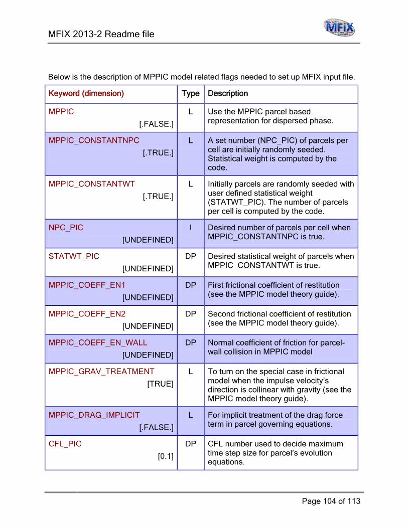
MFIX 2013-2 Readme file
Page 104 of 113
Below is the description of MPPIC model related flags needed to set up MFIX input file.
Keyword (dimension) Type Description
MPPIC
[.FALSE.]
L Use the MPPIC parcel based representation for dispersed phase.
MPPIC_CONSTANTNPC
[.TRUE.]
L A set number (NPC_PIC) of parcels per cell are initially randomly seeded. Statistical weight is computed by the code.
MPPIC_CONSTANTWT
[.TRUE.]
L Initially parcels are randomly seeded with user defined statistical weight (STATWT_PIC). The number of parcels per cell is computed by the code.
NPC_PIC
[UNDEFINED]
I Desired number of parcels per cell when MPPIC_CONSTANTNPC is true.
STATWT_PIC
[UNDEFINED]
DP Desired statistical weight of parcels when MPPIC_CONSTANTWT is true.
MPPIC_COEFF_EN1
[UNDEFINED]
DP First frictional coefficient of restitution (see the MPPIC model theory guide).
MPPIC_COEFF_EN2
[UNDEFINED]
DP Second frictional coefficient of restitution (see the MPPIC model theory guide).
MPPIC_COEFF_EN_WALL
[UNDEFINED]
DP Normal coefficient of friction for parcel-wall collision in MPPIC model
MPPIC_GRAV_TREATMENT
[TRUE]
L To turn on the special case in frictional model when the impulse velocity’s direction is collinear with gravity (see the MPPIC model theory guide).
MPPIC_DRAG_IMPLICIT
[.FALSE.]
L For implicit treatment of the drag force term in parcel governing equations.
CFL_PIC
[0.1]
DP CFL number used to decide maximum time step size for parcel’s evolution equations.
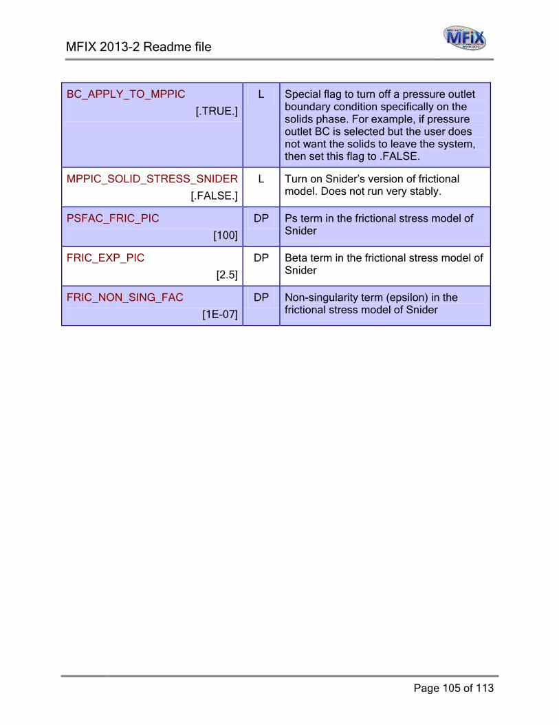
MFIX 2013-2 Readme file
Page 105 of 113
BC_APPLY_TO_MPPIC
[.TRUE.]
L Special flag to turn off a pressure outlet boundary condition specifically on the solids phase. For example, if pressure outlet BC is selected but the user does not want the solids to leave the system, then set this flag to .FALSE.
MPPIC_SOLID_STRESS_SNIDER
[.FALSE.]
L Turn on Snider’s version of frictional model. Does not run very stably.
PSFAC_FRIC_PIC
[100]
DP Ps term in the frictional stress model of Snider
FRIC_EXP_PIC
[2.5]
DP Beta term in the frictional stress model of Snider
FRIC_NON_SING_FAC
[1E-07]
DP Non-singularity term (epsilon) in the frictional stress model of Snider
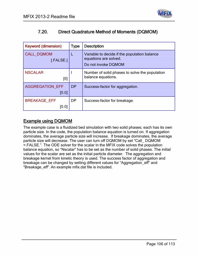
MFIX 2013-2 Readme file
Page 106 of 113
7.20. Direct Quadrature Method of Moments (DQMOM)
Keyword (dimension) Type Description
CALL_DQMOM
[.FALSE.]
L Variable to decide if the population balance equations are solved.
Do not invoke DQMOM
NSCALAR
[0]
I Number of solid phases to solve the population balance equations.
AGGREGATION_EFF
[0.0]
DP Success-factor for aggregation.
BREAKAGE_EFF
[0.0]
DP Success-factor for breakage.
Example using DQMOM The example case is a fluidized bed simulation with two solid phases; each has its own particle size. In the code, the population balance equation is turned on. If aggregation dominates, the average particle size will increase. If breakage dominates, the average particle size will decrease. The user can turn off DQMOM by set “Call_ DQMOM =.FALSE.”. The ODE solver for the scalar in the MFIX code solves the population balance equation, so “Nscalar” has to be set as the number of solid phases. The initial values for the scalar are set as the initial particle diameter. The aggregation and breakage kernel from kinetic theory is used. The success factor of aggregation and breakage can be changed by setting different values for “Aggregation_eff” and “Breakage_eff”. An example mfix.dat file is included.

MFIX 2013-2 Readme file
Page 107 of 113
7.21. Quadrature Method of Moments (QMOM) Please refer to the following document for a brief description of the implementation and utilization of the quadrature method of moments (QMOM): A. Passalacqua, and R. O. Fox, “Documentation of open-source MFIX-QMOM software for gas-solids flows”, available from https://mfix.netl.doe.gov/documentation/qmomk doc_2012-1.pdf
7.22. Cohesion Model in DEM Cohesive interparticle forces represent an addition to the discrete-particle simulation. The raw code for this addition was located in the mfix/model/cohesion directory. These forces can be implemented using both a square-well model and a Hamaker van der Waals model. Cohesive forces are turned-on by setting the logical variable “USE_COHESION” equal to true in the mfix.dat file.
Square-Well model
The nature of the square-well model is determined by the well width (router) and the well depth (D). Both of these parameters are specified in the mfix.dat file. Furthermore, the simulation is set up to use a separate set of square-well parameters with particle-particle interactions and particle-wall interactions. Generally, the well depth is set to be twice as large for particle-wall interactions to be consistent with the increased surface contact that would exist in such interactions.
Within the square well model, cohesive interactions are implemented as instantaneous momentum impulses (J*) resulting in a change in particle velocity as shown below:
,*ij*pre,ipost,i Jmm kvv
−= (1)
where m is the particle mass, pre,iv is the pre-interaction velocity, post,iv is the post-
interaction velocity and ,*ijk
is the unit vector connecting the particle centers. This
treatment leads to three types of cohesive interactions in the square-well model: approaching cohesive interactions, escaping cohesive interactions and capture cohesive interactions. The momentum impulse during each of these interactions can be calculated by solving the momentum balance along with the stipulation that the total kinetic energy of the two-particle system changes by the depth of the square well (D). This treatment leads to the following expressions for the momentum impulse in each type of interaction:
( )
⋅+−⋅=
2
114
2 a,ij,ija,ij,ijapp,coh vkmDvkmJ
(2)

MFIX 2013-2 Readme file
Page 108 of 113
( )
−⋅+⋅=
mDmJ c,ij,ijc,ij,ijesc,coh
42
2
33 vkvk (3)
( )c,ij,ijcap,coh vkmJ ⋅= 3 (4)
Because cohesive interactions are implemented only once on approach and once as the particles depart, the identification of a square-well interaction cannot be done simply using the separation distance. Special book-keeping is employed to ensure that square-well cohesive interactions are implemented only during the time step when the well-widths first become overlapped for approaching interactions and when they first become un-overlapped for departing interactions. This book-keeping involves recording a “list of links” for each particle. Two particles are considered “linked” is their separation distance is less than the width of their square-wells (the square-wells overlap). The list of links is updated at every cohesive interaction. Cohesive square-well interactions are recognized using both the list of links and the particle separation distance at each. For example, an approaching cohesive interaction is only implemented if two particles overlap their square-wells, yet they are not on their respective list of links. The particles will be added to each list during the interaction and at the next time step, they may still have overlapped square-wells, but an interaction will not be implemented because they particles are already on their respective list of links. A similar algorithm is used to identify departing interactions.
Hamaker model
The Hamaker model for van der Waals forces predicts the cohesive force between equal-sized, spherical particles according to the following equation [1]:
212HAr
F innervdW = (5)
where innerr is the particle radius; A is the Hamaker constant, which is specific to a given
material and has typical values on the order of 10-20 J; and H is the minimum surface-to-surface separation distance between two particles i and j:
( ) ( ) innerjiji ryyxxH 222 −−+−= (6)
The corresponding cohesive force between a spherical particle and a flat wall is [1]:
26HrA
F innerwallwall,vdW = (7)
For both of these expressions, the cohesive force approaches infinity as the separation distance approaches zero. This singularity incurred at particle contact is avoided by
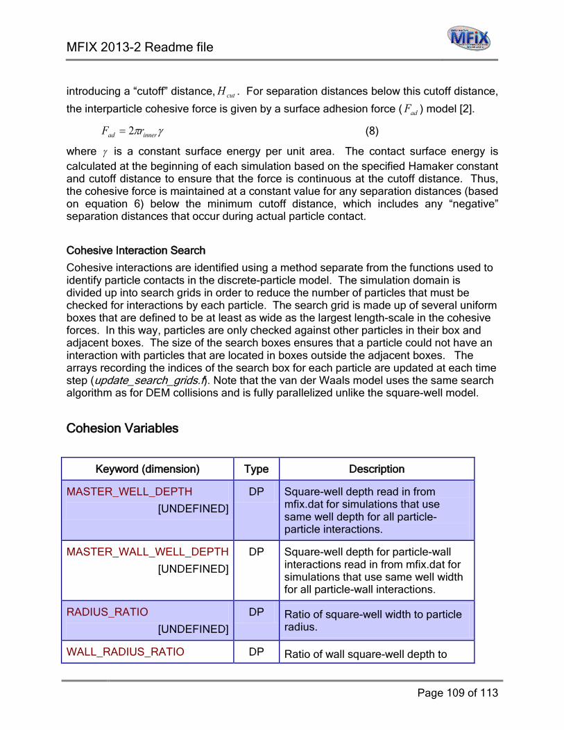
MFIX 2013-2 Readme file
Page 109 of 113
introducing a “cutoff” distance, cutH . For separation distances below this cutoff distance,
the interparticle cohesive force is given by a surface adhesion force ( adF ) model [2].
γπ innerad rF 2= (8)
where γ is a constant surface energy per unit area. The contact surface energy is calculated at the beginning of each simulation based on the specified Hamaker constant and cutoff distance to ensure that the force is continuous at the cutoff distance. Thus, the cohesive force is maintained at a constant value for any separation distances (based on equation 6) below the minimum cutoff distance, which includes any “negative” separation distances that occur during actual particle contact.
Cohesive Interaction Search
Cohesive interactions are identified using a method separate from the functions used to identify particle contacts in the discrete-particle model. The simulation domain is divided up into search grids in order to reduce the number of particles that must be checked for interactions by each particle. The search grid is made up of several uniform boxes that are defined to be at least as wide as the largest length-scale in the cohesive forces. In this way, particles are only checked against other particles in their box and adjacent boxes. The size of the search boxes ensures that a particle could not have an interaction with particles that are located in boxes outside the adjacent boxes. The arrays recording the indices of the search box for each particle are updated at each time step (update_search_grids.f). Note that the van der Waals model uses the same search algorithm as for DEM collisions and is fully parallelized unlike the square-well model.
Cohesion Variables
Keyword (dimension) Type Description
MASTER_WELL_DEPTH
[UNDEFINED]
DP Square-well depth read in from mfix.dat for simulations that use same well depth for all particle-particle interactions.
MASTER_WALL_WELL_DEPTH
[UNDEFINED]
DP Square-well depth for particle-wall interactions read in from mfix.dat for simulations that use same well width for all particle-wall interactions.
RADIUS_RATIO
[UNDEFINED]
DP Ratio of square-well width to particle radius.
WALL_RADIUS_RATIO DP Ratio of wall square-well depth to

MFIX 2013-2 Readme file
Page 110 of 113
[UNDEFINED] particle radius.
USE_COHESION
[.FALSE.]
L Switch to turn cohesion on and off.
SQUARE_WELL
[.FALSE.]
L Switch to turn square well on and off.
COHESION_DEBUG
[UNDEFINED_I]
I Flag to turn on output lines for debugging cohesive simulation.
VAN_DER_WAALS
[.FALSE.]
L Flag to turn on the use Hamaker van der Waals forces.
HAMAKER_CONSTANT
[UNDEFINED]
DP Hamaker constant used for particle-particle interactions
VDW_INNER_CUTOFF
[UNDEFINED]
DP Minimum separation distance below which van der Waals forces are calculated using a surface adhesion model.
VDW_OUTER_CUTOFF
[UNDEFINED]
DP Maximum separation distance above which van der Waals forces are not implemented.
WALL_HAMAKER_CONSTANT
[UNDEFINED]
DP Hamaker constant used in particle-wall interactions.
WALL_VDW_INNER_CUTOFF
[UNDEFINED]
DP Minimum separation distance below which van der Waals forces are calculated using a surface adhesion model (particle-wall interactions).
WALL_VDW_OUTER_CUTOFF
[UNDEFINED]
DP Maximum separation distance above which van der Waals forces are not implemented (particle-wall interactions).
ASPERITIES
[0.0]
DP Mean radius of surface asperities that influence the cohesive force following a model by Rumpf (1990).

MFIX 2013-2 Readme file
Page 111 of 113
7.23. Cartesian grid
A new capability, called Cartesian grid cut-cell technique has been implemented in MFIX, which allows the definition of curved or sloping boundaries, instead of the usual stair-step representation. Computational cells are truncated at the wall to conform to the shape of the boundaries. When a face is truncated, the velocity node is moved to the center of the face. The cell truncation introduces an additional face, called the cut face. Face surface areas and cell volumes are updated based on the shape of the cut cell. The contribution of the new cut face is added to the computation. The data can be saved in a vtk file for post-processing purpose.
A detailed user guide named Cartesian_grid_user_guide.pdf is located in mfix/doc directory. It should be read prior to utilizing the Cartesian grid option to get familiar with this technique, and associated keywords . This file is also available online at https://mfix.netl.doe.gov/documentation/Cartesian_grid_user_guide.pdf.

MFIX 2013-2 Readme file
Page 112 of 113
8. Mailing lists
Several mailing lists are available to communicate among MFIX users and developers. When your subscription to MFIX is accepted, you are automatically added to the mfix-news mailing list, where important announcements about MFIX are shared with the MFIX community.
The most widely used mailing list is mfix-help, which allows users to post questions and eventually help other users with similar issues.
The mailing list home page is located at https://mfix.netl.doe.gov/sympa. Click on the “List of lists” tab to view all available mailing lists. Most of them have a very low bandwidth, and most users only subscribe to the mfix-help list.
Once you subscribe to a list, you can send/receive messages to/from the MFIX community. You can also search archived messages to see if there is already a solution to a common problem.
There are many options to manage your subscription, including subscribing, unsubscribing, and choosing the delivery mode.
Please visit https://mfix.netl.doe.gov/sympa/help/user to view the mailing list user guide.
Mailing list etiquette:
1) Please allow sufficient time (say 2 to 3 business days) for MFIX developers and users to reply before posting unanswered questions again.
2) Unless prior arrangement has been made with a given MFIX developer, do not send requests directly to the developer, but send the request to the appropriate mailing list instead. This ensures proper archiving of the thread and provides better opportunity for everyone to reply. Follow-up questions should also be sent to the mailing list.
3) Do not ask for a copy of a reference, e.g., a journal article. 4) Prior to submitting help requests regarding MFIX installation or compilation
issues, please check the archives of mfix-help and if you are still having a problem, email [email protected] by providing the following important details in your message after the description of the problem encountered:
a. MFIX version you are trying to install or run

MFIX 2013-2 Readme file
Page 113 of 113
b. Some details on your operating system environment (for Linux: copy and paste the response of uname –a command, Linux distribution name and version also)
c. Your compiler name and version number (e.g. ifort –v will give the version number for Intel fortran compiler)
d. Output for your $PATH environment (in csh type echo $PATH) e. Your MPI library name and version number (if compilations problem with
DMP mode encountered but make sure you can compile and run a simple hello world type MPI program with your current installation) Also please provide hardware details such as number of cores per socket in your system (or send the output for “cat /proc/cpuinfo“ and how many cores you are trying to utilize.
9. User contribution If you wish to contribute to the development of MFIX, please contact the MFIX team at [email protected]. We are looking for simulation results (figures, animations, input files, user-defined subroutines), and new models that could benefit the entire MFIX community. If you have written or know any publication that uses MFIX, please let us know and we will post the citation on the website. Proper credit will be given to all contributors.
Common reasons you may not receive an answer to your request
1. You did not subscribe to the mailing list. 2. You sent the request to an individual and not to the mailing list. 3. Your question has already been answered and is available in the
archive. 4. You did not provide sufficient description of your problem (saying “It
doesn’t work” is not useful). 5. Your question is outside the scope of the mailing list.