Annals of Glaciology 16 1992 © International Glaciological Society

Reactions of a calving glacier to large changes in water

level

TRON LAUMANN AND BJ0RN WOLD Norwegian Water Resources and Energy Administration, P.O.Box 5091, Maj., N-0301 Oslo 3, Norway

ABSTRACT. Austdalsvatn in western Norway was regulated in 1988 as a reservoir for a hydropower development. From a pre-1988 water level of 1157 m a.s.!. the new water level will vary more or less annually from 1170 to 1200 m a.s.!. The outlet glacier Austdalsbreen calves into this reservoir. About 1600 m up-valley from its terminus the glacier flows over a bedrock riegel that is, at its lowest point, '" 15 m above the projected maximum lake level of 1200 m. As a result of the increase in water level, the surface velocity near the front has increased from about 0.07 to 0.13md-1

.

Calculations suggest that the glacier terminus will retreat about 750 m in 50 years. The measured response of the glacier terminus for the first three years is in good agreement with the simulations.

INTRODUCTION previous normal water level in the lake was 1157 m a.s.!. An outlet glacier, Austdalsbreen, which drains the northern part of J ostedalsbreen, terminates in the reservoir (Fig. I).

As part of the construction of the Jostedal hydropower station in western Norway, the water level in Austdals­vatn can vary between 1130 and 1200 m a.s .l. The

NORWAY

Radio-echo measurements (Sretrang, 1987) revealed

o 500 m ... ' --'_ -'---'---10._,

N

t

Fig. 1. Map of Austdalsbreen from 1988 showing positions of stakes with measured velocities, various front positions and the subglacial bed topography near the terminus.

158

·5

m a.s.1

--1989

·4 ·3 ·2 ·1 0 2

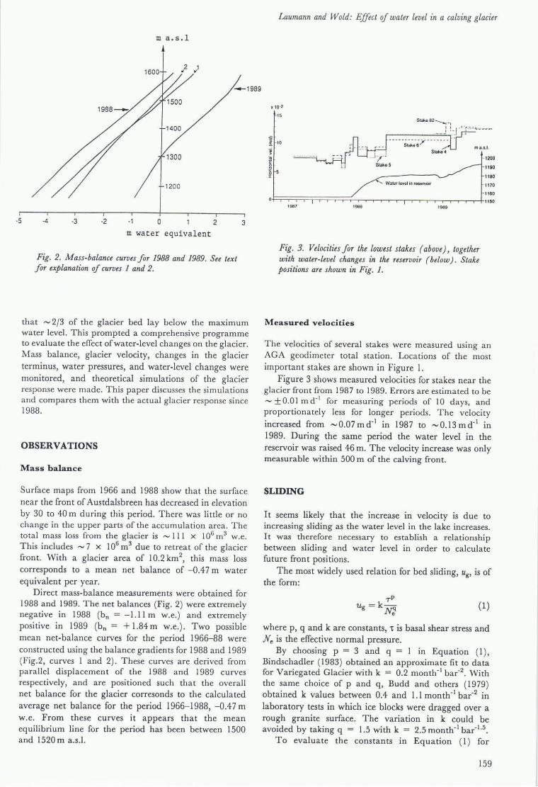
m water equivalent

Fig. 2. Mass-balance curves for 1988 and 1989. See text for explanation of curves 1 and 2.

3

that ~ 2/3 of the glacier bed lay below the maximum water level. This prompted a comprehensive programme to evaluate the effect of water-level changes on the glacier. Mass balance, glacier velocity, changes in the glacier terminus, water pressures, and water-level changes were monitored, and theoretical simulations of the glacier response were made. This paper discusses the simulations and compares them with the actual glacier response since 1988.

OBSERVATIONS

Mass balance

Surface maps from 1966 and 1988 show that the surface near the front of Austdalsbreen has decreased in elevation by 30 to 40 m during this period. There was little or no change in the upper parts of the accumulation area. The total mass loss from the glacier is ~ III X 106 m3 w.e. This includes ~ 7 x 106 m3 due to retreat of the glacier front. With a glacier area of 10.2 km2

, this mass loss corresponds to a mean net balance of -0.47 m water equivalent per year.

Direct mass-balance measurements were obtained for 1988 and 1989. The net balances (Fig. 2) were extremely negative in 1988 (bn = -1.11 m w.e.) and extremely positive in 1989 (bn = + 1.84 m w.e.). Two possible mean net-balance curves for the period 1966-88 were constructed using the balance gradien ts for 1988 and 1989 (Fig.2, curves 1 and 2). These curves are derived from parallel displacement of the 1988 and 1989 curves respectively, and are positioned such that the overall net balance for the glacier corresonds to the calculated average net balance for the period 1966-1988, -0.47 m w.e. From these curves it appears that the mean equilibrium line for the period has been between 1500 and 1520 m a.s.L

Laumann and Wold: Effect of water level in a calving glacier

x 10 .2

15

l ID

~ 5 !l 'g r

Slake 82 ---I _, t I • _, - r :: . ~ \. .. " ' ~ ' '''' •

. _._ .! '-:.i

Waler lovel in reservoir

ma.s.l.

1200

1190

1180

1170

1160

.j:::::;=;:::::;::::;=::;=;=;C=;:=;:=~.--.--'--.--'-'-'r-r--'.-'--r-r-r--r-.--l, 11 SO 1987 1988 1989

Fig. 3. Velocities for the lowest stakes (above), together with water-level changes in the reservoir (below). Stake positions are shown in Fig. 1.

Measured velocities

The velocities of several stakes were measured using an AGA geodimeter total station. Locations of the most important stakes are shown in Figure 1.

Figure 3 shows measured velocities for stakes near the glacier front from 1987 to 1989. Errors are estimated to be - ±0.01 md'l for measuring periods of 10 days, and proportionately less for longer periods. The velocity increased from ~0.07md·l in 1987 to ~O.l3md·l in 1989. During the same period the water level in the reservoir was raised 46 m. The velocity increase was only measurable within 500 m of the calving front.

SLIDING

It seems likely that the increase in velocity is due to increasing sliding as the water level in the lake increases. It was therefore necessary to establish a relationship between sliding and water level in order to calculate future front positions.

The most widely used relation for bed sliding, ug , is of the form:

r P ug=k m (1)

where p, q and k are constants, 't is basal shear stress and Ne is the effective normal pressure.

By choosing p = 3 and q = 1 in Equation (1), Bindschadler (1983) obtained an approximate fit to data for Variegated Glacier with k = 0.2 month,l bar'2. With the same choice of p and q, Budd and others (1979) obtained k values between 0.4 and 1.1 month'l bar·2 in laboratory tests in which ice blocks were dragged over a rough granite surface. The variation in k could be avoided by taking q = 1.5 with k = 2.5 month'l bar'1.5.

To evaluate the constants in Equation (I) for

159

Laumann and Wold: Effect of water level in a calving glacier

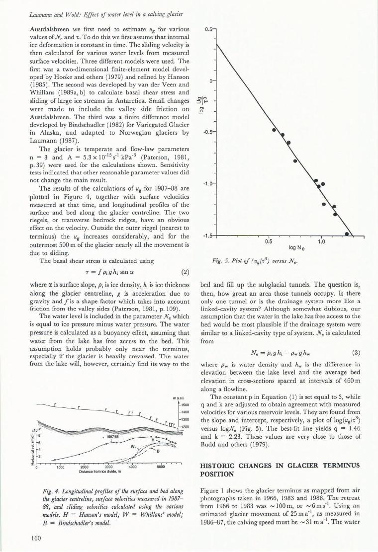
Austdalsbreen we first need to estimate ug for various 0.5

values of Ne and 'to To do this we first assume that internal ice deformation is constant in time. The sliding velocity is then calculated for various water levels from measured surface velocities. Three different models were used. The first was a two-dimensional finite-element model devel-oped by Hooke and others (1979) and refined by Hanson ( 1985). The second was developed by van der Veen and Whillans (1989a, b) to calculate basal shear stress and sliding of large ice streams in Antarctica. Small changes were made to include the valley side friction on Austdalsbreen. The third was a finite difference model developed by Bindschadler (1982) for Variegated Glacier in Alaska, and adapted to Norwegian glaciers by Laumann (1987).

The glacier is temperate and flow-law parameters n = 3 and A = 5.3 X 1O-15 s- 1 kPa-3 (Paterson, 1981, p.39) were used for the calculations shown. Sensitivity tests indicated that other reasonable parameter values did not change the main result.

The results of the calculations of ug for 1987-88 are plotted in Figure 4, together with surface velocities measured at that time, and longitudinal profiles of the surface and bed along the glacier centreline. The two riegels, or transverse bedrock ridges, have an obvious effect on the velocity. Outside the outer riegel (nearest to terminus) the ug increases considerably, and for the outermost 500 m of the glacier nearly all the movement is due to sliding.

The basal shear stress is calculated using

T = f Pighi sin a (2)

where r:x is surface slope, Pi is ice density, hi is ice thickness along the glacier centreline, g is acceleration due to gravity and f is a shape factor which takes into account friction from the valley sides (Paterson, 1981, p. 109).

The water level is included in the parameter Ne which is equal to ice pressure minus water pressure. The water pressure is calculated as a buoyancy effect, assuming that water from the lake has free access to the bed. This assumption holds probably only near the terminus, especially if the glacier is heavily crevassed. The water from the lake will, however, certainly find its way to the

I ~

6

g ~ 2

i~~~-.~~~~~~~~~~/,-~~~-.~~ o 1000 2000 3000 4000 SOOO

Distance lrom ice divide, m

160

Fig. 4. Longitudinal profiles of the surface and bed along the glacier centreline, surface velocities measured in 1987-88, and sliding velocities calculated using the various models. H = Hanson's model; W = Whillans' model; B = Bindschadler's model.

o

-0.5

-1.0

0.5 log Ne

Fig. 5. Plot of (ug /-r;3) versus Ne.

1.0

bed and fill up the subglacial tunnels. The question is, then, how great an area those tunnels occupy. Is there only one tunnel or is the drainage system more like a linked-cavity system? Although somewhat dubious, our assumption that the water in the lake has free access to the bed would be most plausible if the drainage system were similar to a linked-cavity type of system. Ne is calculated from

(3)

where Pw is water density and hw is the difference in elevation between the lake level and the average bed

elevation in cross-sections spaced at intervals of 460 m along a flowline.

The constant p in Equation (1) is set equal to 3, while q and k are adjusted to obtain agreement with measured velocities for various reservoir levels. They are found from the slope and intercept, respectively, a plot of log(ug/'t

3)

versus 10gNe (Fig. 5). The best-fit line yields q = 1.46 and k = 2.23. These values are very close to those of Budd and others (1979).

HISTORIC CHANGES IN GLACIER TERMINUS POSITION

Figure 1 shows the glacier terminus as mapped from air photographs taken in 1966, 1983 and 1988. The retreat from 1966 to 1983 was ",lOOm, or ",6ms-1

• Using an estimated glacier movement of 25 m a-I, as measured in 1986-87, the calving speed must be ",31 m a-I. The water

depth is 7 to 10 m. The empirical relation found by Funk and Rothlisberger (1989) gives a calving speed of 15 to 30 m a-I for these depths, which is in reasonable agreement with that inferred from the retreat rate.

From 1983 to 1988 several calving bays were created. Calving rates vary considerably along the glacier terminus during this period, which makes the use of empirical average equations difficult. Generally the calving rate for this period has been slightly higher than calculated before the increase in water level, probably due mainly to the influence of changing water depth and of the subglacial and proglacial rivers flowing approxi­mately parallel to the calving face.

SIMULATIONS

Models and scenarios

Calculations of possible changes in the terminus of Austdalsbreen have been made using a simple steady­state simulation and a dynamic model. The steady-state simulation is similar to the study made for a Swiss glacier

ma.s.1.

1600,..~~~

1500

1400

1300

1200

----

1100~-r'-~~-r'-ro-'-''-,,-'-',-,,-'-''-,,-', 1100 2000 4000 6000

Dislance from ice divide, m

Fig. 6. Longitudinal profiles along the centreline. From maps (1966 and 1988) and calculated with the dynamic model for the 1988 situation.

VELOC ln QI S TRIBU1ION F OR 19 9'

. 0

;/ v.-- I~ r'-

V :.---1--------

// / '

V /.

20

/'

° - o 1000 2000 . 000 5000 6000

0 15 t At ICE f"ROM t CE 0 I V I DE/BERGSC~RUNO HE 1 ER S

Fig. 7. Calculated (solid line) and measured (triangles) velocities along the centreline. Vertical lines are boundaries between the model sections.

Laumann and Wold: Effect of water level in a calving glacier

by Funk and Rothlisberger (1989), and results for Austdalsbreen have previously been published by Hooke and others (1989). The most important assumption in these calculations was that the surface profile is a steady­state profile, and that the mass balance will not change substantially. Other important factors not taken into account are calving, when the glacier terminus begins to

float, increasing glacier movement due to reduced friction, and large variations in calving rate due to large water-level variations.

The dynamic model is developed for Variegated Glacier by Bindschadler (1982) and adapted to Norwe­gian glaciers by Laumann (1987), Sliding is calculated using Equation (1), and calving is calculated using Funk and Rothlisberger's (1989) empirical relationship which, as noted gives reasonable agreement for calving from 1966 to 1988. The model is calibrated using surface profile changes between 1966 and 1988 (Fig. 6) and measured velocities from 1987 (Fig. 7).

Simulations are made for three climate scenarios: (1) Equilibrium net balance (bn = 0), (2) net balance equal to the 1966-88 mean (bn = -0.47), and (3) a climate influenced by increasing greenhouse gases up to a doubling of CO2 by 2030 AD. The third scenario is based on that reported by a Norwegian expert team in a report to an Interdepartmental Group for Assessing Conse­quences of Climate Changes (Eliassen and others, unpublished; Sa:lthun and others, 1990). Scenarios are given for temperature and precipitation . The one considered to be most likely predicts an increase in temperature of 1.5 to 3.5°, and an increase in precipita­tion of 7 to 8%.

For each scenario, simulations are made for two constant water levels (1157 and 1200 m a.s.l. ), and for the normal expected yearly water-level variation between 1170 and 1200 m a.s.!. The highest level is in the autumn and the lowest level in spring.

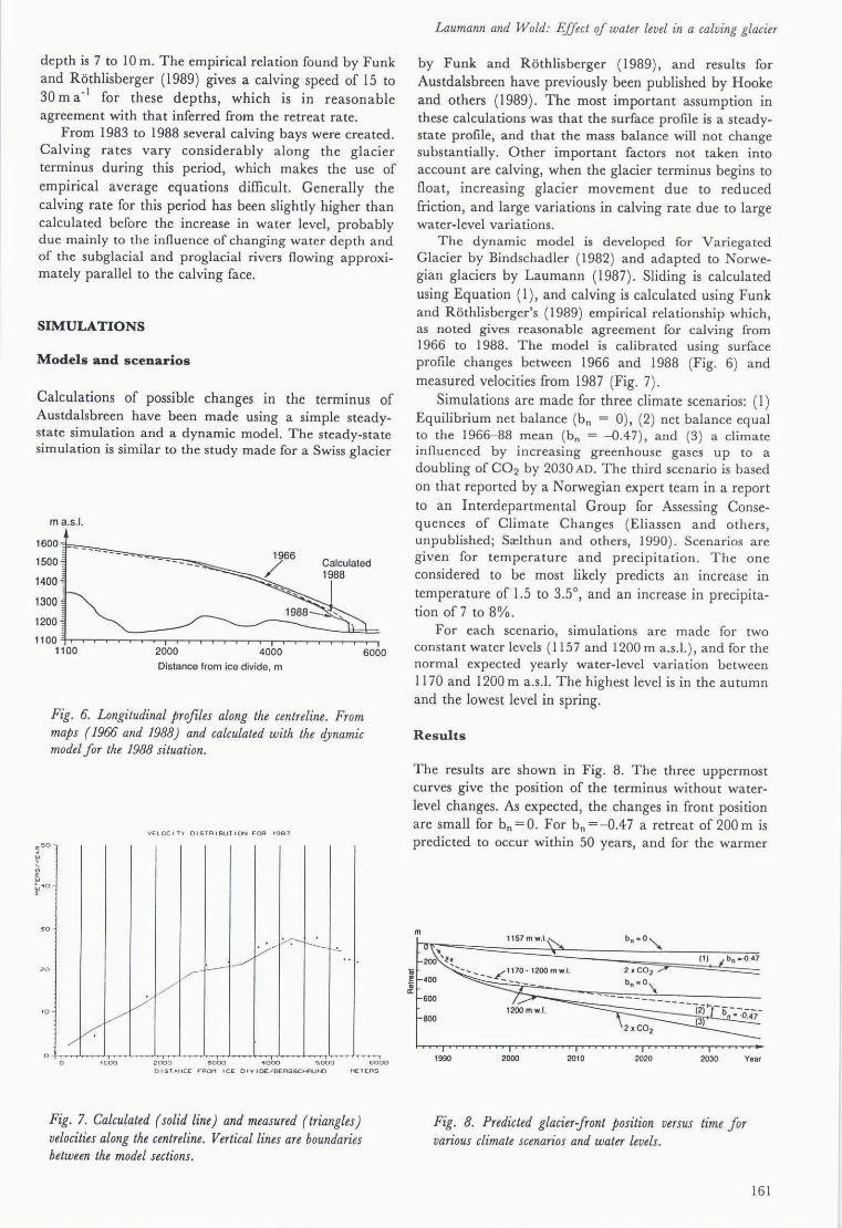
Results

The results are shown in Fig. 8. The three uppermost curves give the position of the terminus without water­level changes. As expected, the changes in front position are small for bn = O. For bn = -0.4 7 a retreat of 200 m is predicted to occur within 50 years, and for the warmer

m

10

~ a:

1157mw.I. b •• O"" .. (1) ,.: bn • .0.47 200 \~.

-'- ____ /1170, 12oomw.L 2ICC02 :> , =

400 ----- bn .0\

600 1200 mw.I.

800

1990 2000 2010 2020 2030 Year

Fig. 8. Predicted glacier-front position versus time for various climate scenarios and water levels.

161

Laumann and Wold: Effect of water level in a calving glacier

climate the retreat seems to be an additional 50 m. The increase in water level is of great importance. For

bn = 0 and 1200 m a.s.l. water level, the simulation gives 600 m retreat in 50 years, with 80% of this during the first ten years. This is in good agreement with the estimate of Hooke and others (1989) based on similar assumptions.

The influence of climate change on the front position is predicted to be less than the influence of increased calving. This is illustrated by the curves for 1200 m water level, which are identical during the first five years and then diverge. The retreat for bn = -0.47 is 900 m, and for 2 X CO2 it is 1000 m in 50 years.

The broken line in Fig. 8 gives the result of varying water level with bn = -0.47. In this case the glacier is predicted to retreat 750 m in 50 years. This is considered to be the most probable result of water-level regulation.

The water-level changes affect not only the outermost parts of the glacier, but also should be seen further up­glacier. The surface should be somewhat lowered due to the increased velocity, and the profile is expected to become steeper as the glacier tries to adapt to the increasing calving rate (Fig. 9).

COMPARISON WITH OBSERVATIONS

The water level started to rise inJune 1988 (Fig. 3). The retreat of the terminus from spring 1988 to spring 1989 averaged 75 m. The velocity near the front during during the same period increased from 25 to 36 m a-I, which gives a new calving rate of III m a-I.

The water-level rise continued during June and July 1989. This was expected to have a large influence on the calving activity. However, the calving activity during this period was very low. The position of the terminus did not change from spring to autumn 1989. Possibly the low calving rate was due to the cold summer, in which the lake-ice cover did not break up until the middle of August, or possibly the glacier was stuck in deep sediment layers. However, during the flooded conditions in autumn

some large pieces started to break off, the largest with an estimated volume of 30000 m3

. The total retreat of the terminus from spring 1989 to autumn 1990 was ~ 100 m.

The measured response of the glacier terminus for the first three years, plotted in Fig. 8 (crosses), is in good agreement with the simulations.

ma.s.I. '600

DiSlance trom ice divide. m

Fig. 9. Longitudinal profile measured in 1986, and simulated for 2030 A.D. with bn = -{}.47. (1 is water level 1157 m a.s.l, 2 is expected normal yearly water-level variations, 3 is water level 1200 m a.s.l.)

162

ACKNOWLEDGEMENTS

This work was financed by the Norwegian State Power Board and the Norwegian Water Resources and Energy Administration. Field work was carried out by several staff members of our department, who also helped by other ways. We thank them all, and in particular Mike Kennett and Roger LeB. Hooke for valuable discussions.

REFERENCES

Bindschadler, R. 1982. A numerical model of temperate glacier flow applied to the quiescent phase of a surge­type glacier. ]. Glaciol., 28 (99), 239- 265.

Bindschadler, R. 1983. The importance of pressurized subglacial water in separation and sliding at the glacier bed. J. Glaciol., 29(101), 3-19.

Budd, W. F., P. L. Keage and N. A. Blundy. 1979. Empirical studies of ice sliding. ]. Glaciol., 23 (89), 157-170.

Eliassen, A. and 6 others. Unpublished. Klimaendringer i Norge ved 0kt drivhuseffekt. Rapport til Milj0vernde­partementets klimautredningsgruppe.

Funk, M. and H. Rothlisberger. 1989. Forecasting the effects of a planned reservoir which will partially flood the tongue of Unteraargletscher in Switzerland. Ann. Glaciol., 13, 76-81.

Hanson, B. H . 1985. Climate sensitivity of a numerical model of ice-sheet dynamics. (Ph.D.thesis, University of Minnesota. National Center for Atmospheric Research. Cooperative Thesis 9l. )

Hooke, R. LeB., C. F. Raymond, R. L. Hotchkiss and R.J. Gustafson. 1979. Calculations of velocity and temperature in a polar glacier using the finite-element method. J. Glaciol., 24 (90), 131-146.

Hooke, R. LeB., T. Laumann and M. I. Kennett. 1989. Austdalsbreen, Norway: expected reaction to a 40 m increase in water level in the lake into which the glacier calves. Cold Reg. Sci. Technol., 17(2), 113-126.

Laumann, T. 1987. En dynamisk modell for isbreers bevegelse. Oslo, Norges Vassdrags- og Energiverk. Vassdragsdir­ektoratet. Hydrologisk avdeling. (V-publikasjon 8.)

Paterson, W. S. B. 1981. The physics of glaciers. Second edition. Oxford, etc., Pergamon Press.

Sa:lthun, N . R. and 6 others. 1990. Klimaendringer og vannressurser. Bidrag til den interdepartementale klimautred­ningen. Oslo, Norges Vassdrags- og Energiverk. Vassdragsdirektoratet. Hydrologisk avdeling. (V-pub­likasjon 30.)

Sa:trang, A. C. 1987. Kartlegging av istykkelse pd nordre Jostedalsbreen. Oslo, Norges Vassdrags- og Energiverk. (Oppdragsrapport 8-87 .)

Van der Veen, C.]. and I. M. WhiUans. 1989a. Force budget: I. Theory and numerical methods. ] . Glaciol., 35(119),53-60.

Van der Veen, G.]. and 1. M Whillans. 1989b. Force budget: 11. Application to two-dimensional flow along Byrd Station Strain Network, Antarctica. J. Glaciol., 35(119),61-67.

The accuracy of references in the text and in this list is the responsibility of the author/s, to whom queries should be addressed.