Reachability Analysis of Cyber-Physical Systems using

Symbolic-Numeric Techniques

by

Aditya Krishna Zutshi

B.E., Manipal University, 2007

M.S., University Colorado, 2011

A thesis submitted to the

Faculty of the Graduate School of the

University of Colorado in partial fulfillment

of the requirements for the degree of

Doctor of Philosophy

Department of Electrical, Computer, and Energy Engineering

2016

This thesis entitled:Reachability Analysis of Cyber-Physical Systems using Symbolic-Numeric Techniques

written by Aditya Krishna Zutshihas been approved for the Department of Electrical, Computer, and Energy Engineering

Prof. Sriram Sankaranarayanan

Prof. Fabio Somenzi

Prof. Bor-Yuh Evan Chang

Dr. Jyotirmoy V. Deshmukh

Dr. James Kapinski

Date

The final copy of this thesis has been examined by the signatories, and we find that both the content and theform meet acceptable presentation standards of scholarly work in the above mentioned discipline.

iii

Zutshi, Aditya Krishna (Ph.D., Electrical Engineering)

Reachability Analysis of Cyber-Physical Systems using Symbolic-Numeric Techniques

Thesis directed by Prof. Sriram Sankaranarayanan

In this thesis, we address the problem of reachability analysis in cyber-physical systems. These are

systems engineered by interfacing computational components with the physical world. They provide partially

or fully automated safety-critical services in the form of medical devices, autonomous vehicles, avionics and

power systems.

We propose techniques to reason about the reachability of such systems, and provide methods for

falsifying their safety properties. We model the cyber component as a software program and the physical

component as a hybrid dynamical system. Unlike model based analysis, which uses either a purely symbolic

or a numerical approach, we argue in favor of using a combination of the two. We justify this by noting that

the software program running on a computer is completely specified and has precise semantics. In contrast,

the model of the physical system is only an approximation. Hence, we treat the former as a white box, but

treat the latter as a black box.

Using symbolic methods for the cyber components and numerical methods for hybrid systems, we

carefully capture the complex behaviors of software programs and circumvent the difficulty in analyzing

complex models developed through first principles. To combine the two techniques, we use a Counterexample

Guided Abstraction Refinement (CEGAR) framework. Furthermore, we explore learning techniques like

regression and piecewise affine modeling to estimate and represent black box hybrid dynamical systems for

the purpose of falsification.

We use prototype implementations to demonstrate the effectiveness of presented ideas. Using non-

trivial benchmarks, we compare their performance against the state of the art. We also comment on their

applicability and discuss ideas for further improvement.

Dedication

To my parents, for their sacrifices, love and encouragement.

To the loving memory of my grandfather.

v

Acknowledgements

First and foremost, I would like to thank my advisor, Prof. Sriram Sankaranarayanan, without whose

encouragement, guidance and support, this thesis would have never taken shape and reached completion.

His broad knowledge and the ability to draw connections between seemingly unrelated concepts has been a

constant source of inspiration.

I would like to thank the committee members for their valuable feedback and their mentorship which

has helped shape not only this thesis, but me as a person. Thanks to Prof. Fabio Somenzi, for introducing me

to ‘formal methods’ through his teachings and for always being available for discussions. Thanks to Prof.

Evan Chang for making the CUPLV lab a fun place to work at. I am grateful to Dr. Jyotirmoy Deshmukh

for encouraging me to be creative, and Dr. James Kapinski for balancing it and keeping me grounded with

real-life examples.

During my first semester, Prof. Aaron Bradley agreed to mentor me and put me on a path to research.

I fondly remember his course ‘Thinking Concurrently’, which I enjoyed like none other. I am indebted to

him for his guidance. I am grateful to Dr. Ashish Tiwari for guiding my research career in the very beginning,

and for being unreasonably patient at answering my numerous questions.

I would like to thank all past and present members of the CUPLV lab for being amazing friends.

Especially, Dr. Aleksandar Chakarov, Dr. Amin Ben Sassi and Yi-Fan Tsai for long discussions and constant

support. Thanks to Prof. Ashutosh Trivedi for impromptu discussions and quick feedbacks on my research.

I would like to thank Dr. Xin Chen, Hadi Ravanbaksh, Dr. Sergio Mover, Dr. Vris Cheung for interesting

discussions over the years.

I am grateful to Prof. Indranil Saha, who has been like an elder brother, providing much needed advice.

vi

I also thank Dr. Nikos Arechiga, Dr. Xioaqing Jin for their friendship and valuable feedback.

Thanks to Dr. Vivek Tiwari, Dr. Rohan Singh and Aditya Bhave for making my years at Boulder

memorable.

Thanks to my wife Vidhya, for supporting me through toughest of the times, my parents for their

constant love and encouragement, and my brother for providing much needed humor in life.

I am indebted to the ECEE Graduate Program Advisor, Adam Sadoff for answering my countless

queries and guiding me effortlessly throughout the years.

I want to mention many others who have influenced this thesis. Discussions with Dr. Bertrand Jeannet,

Dr. Peter Schrammel, Prof. Stefan Ratschan, Jan Kurátko, Prof. Paulo Tabuada, Dr. Hisahiro Ito, Dr. Koichi

Ueda, Dr. Ken Butts and Dr. Tomoyuki Kaga have brought in varied perspectives to my research.

Finally, I gratefully acknowledge the support by the US National Science Foundation (NSF) under the

award numbers CNS-0953941, CNS-1016994, CPS-1035845 and CNS-1319457 and Toyota Engineering and

Manufacturing North America (TEMA).

vii

Contents

Chapter

1 Introduction 1

1.1 Motivation . . . . . . . . . . . . . . . . . . . . . . . . . . . . . . . . . . . . . . . . . . . . 2

1.2 Safety Properties . . . . . . . . . . . . . . . . . . . . . . . . . . . . . . . . . . . . . . . . 2

1.3 Current State of the Art . . . . . . . . . . . . . . . . . . . . . . . . . . . . . . . . . . . . . 3

1.4 System Models . . . . . . . . . . . . . . . . . . . . . . . . . . . . . . . . . . . . . . . . . 3

1.4.1 Sampled Data Control Systems (SDCS) . . . . . . . . . . . . . . . . . . . . . . . . 4

1.4.2 Plant as a Hybrid System . . . . . . . . . . . . . . . . . . . . . . . . . . . . . . . . 5

1.4.3 Controller as a Computer Program . . . . . . . . . . . . . . . . . . . . . . . . . . . 6

1.5 Contributions . . . . . . . . . . . . . . . . . . . . . . . . . . . . . . . . . . . . . . . . . . 6

1.6 Thesis Organization . . . . . . . . . . . . . . . . . . . . . . . . . . . . . . . . . . . . . . . 7

1.7 Publications . . . . . . . . . . . . . . . . . . . . . . . . . . . . . . . . . . . . . . . . . . . 8

2 Background: System Models and Safety 9

2.1 Notation . . . . . . . . . . . . . . . . . . . . . . . . . . . . . . . . . . . . . . . . . . . . . 9

2.2 Dynamical Systems . . . . . . . . . . . . . . . . . . . . . . . . . . . . . . . . . . . . . . . 9

2.2.1 Continuous-time Dynamical Systems . . . . . . . . . . . . . . . . . . . . . . . . . 10

2.2.2 Discrete Event Systems . . . . . . . . . . . . . . . . . . . . . . . . . . . . . . . . . 12

2.2.3 Hybrid Dynamical Systems . . . . . . . . . . . . . . . . . . . . . . . . . . . . . . 13

2.3 Sampled Data Control System (SDCS) . . . . . . . . . . . . . . . . . . . . . . . . . . . . . 16

viii

2.4 Black Box Models . . . . . . . . . . . . . . . . . . . . . . . . . . . . . . . . . . . . . . . 17

2.4.1 Plant Behavioral Model . . . . . . . . . . . . . . . . . . . . . . . . . . . . . . . . 17

2.4.2 Controller . . . . . . . . . . . . . . . . . . . . . . . . . . . . . . . . . . . . . . . . 19

2.5 Behavioral Model of SDCS . . . . . . . . . . . . . . . . . . . . . . . . . . . . . . . . . . . 19

2.6 Reachability Properties . . . . . . . . . . . . . . . . . . . . . . . . . . . . . . . . . . . . . 21

2.7 Related Work . . . . . . . . . . . . . . . . . . . . . . . . . . . . . . . . . . . . . . . . . . 21

2.7.1 Verification . . . . . . . . . . . . . . . . . . . . . . . . . . . . . . . . . . . . . . . 22

2.7.2 Falsification . . . . . . . . . . . . . . . . . . . . . . . . . . . . . . . . . . . . . . . 23

2.7.3 Closed Loop Analysis Techniques . . . . . . . . . . . . . . . . . . . . . . . . . . . 26

3 Segmented Trajectories - A Behavioral Perspective 27

3.1 Introduction . . . . . . . . . . . . . . . . . . . . . . . . . . . . . . . . . . . . . . . . . . . 27

3.2 Trajectory Segments . . . . . . . . . . . . . . . . . . . . . . . . . . . . . . . . . . . . . . 28

3.3 Trajectory Splicing using Optimization . . . . . . . . . . . . . . . . . . . . . . . . . . . . . 32

3.3.1 Problem Setup . . . . . . . . . . . . . . . . . . . . . . . . . . . . . . . . . . . . . 33

3.3.2 Splitting the Optimization Problem . . . . . . . . . . . . . . . . . . . . . . . . . . 34

3.3.3 Evaluation on Navigation Benchmark . . . . . . . . . . . . . . . . . . . . . . . . . 35

3.4 Related Work . . . . . . . . . . . . . . . . . . . . . . . . . . . . . . . . . . . . . . . . . . 37

3.4.1 Qualitative Exploration of Non-Linear Dynamical Systems . . . . . . . . . . . . . . 37

3.4.2 Reachability as a Boundary Value Problem . . . . . . . . . . . . . . . . . . . . . . 39

3.4.3 Trajectory optimization . . . . . . . . . . . . . . . . . . . . . . . . . . . . . . . . . 41

3.5 Summary . . . . . . . . . . . . . . . . . . . . . . . . . . . . . . . . . . . . . . . . . . . . 41

4 Implicit Discrete Abstraction of Black Box Dynamical Systems 43

4.1 Overview . . . . . . . . . . . . . . . . . . . . . . . . . . . . . . . . . . . . . . . . . . . . 43

4.2 Abstractions . . . . . . . . . . . . . . . . . . . . . . . . . . . . . . . . . . . . . . . . . . . 45

4.3 Abstraction as a Reachability Graph . . . . . . . . . . . . . . . . . . . . . . . . . . . . . . 50

4.4 Parameters of the Abstraction (∆ and ε) . . . . . . . . . . . . . . . . . . . . . . . . . . . . 53

ix

4.5 Search for Abstract Counter-examples . . . . . . . . . . . . . . . . . . . . . . . . . . . . . 53

4.5.1 Scatter and Simulate . . . . . . . . . . . . . . . . . . . . . . . . . . . . . . . . . . 55

4.5.2 Analysis of Scatter and Simulate . . . . . . . . . . . . . . . . . . . . . . . . . . . . 57

4.6 Counter-example guided Refinement . . . . . . . . . . . . . . . . . . . . . . . . . . . . . . 59

4.6.1 Asymptotic Analysis of Refinement . . . . . . . . . . . . . . . . . . . . . . . . . . 62

4.7 Summary . . . . . . . . . . . . . . . . . . . . . . . . . . . . . . . . . . . . . . . . . . . . 63

5 Analysis of Sampled Data Control Systems 64

5.1 Overview . . . . . . . . . . . . . . . . . . . . . . . . . . . . . . . . . . . . . . . . . . . . 64

5.2 Symbolic-Numeric Methods . . . . . . . . . . . . . . . . . . . . . . . . . . . . . . . . . . 65

5.3 Symbolic Execution of Programs . . . . . . . . . . . . . . . . . . . . . . . . . . . . . . . . 65

5.4 Example: Thermostat-Heater Temperature Controller . . . . . . . . . . . . . . . . . . . . . 66

5.5 SDCS Model . . . . . . . . . . . . . . . . . . . . . . . . . . . . . . . . . . . . . . . . . . 68

5.6 Software-Centric View of the Controller . . . . . . . . . . . . . . . . . . . . . . . . . . . . 69

5.7 Controller Abstraction . . . . . . . . . . . . . . . . . . . . . . . . . . . . . . . . . . . . . 71

5.8 Closed Loop Execution . . . . . . . . . . . . . . . . . . . . . . . . . . . . . . . . . . . . . 72

5.9 Summary . . . . . . . . . . . . . . . . . . . . . . . . . . . . . . . . . . . . . . . . . . . . 73

6 The Falsification Tool: S3CAM 76

6.1 S3CAM Architecture . . . . . . . . . . . . . . . . . . . . . . . . . . . . . . . . . . . . . . 76

6.2 Tool Implementation . . . . . . . . . . . . . . . . . . . . . . . . . . . . . . . . . . . . . . 78

6.3 Input Description . . . . . . . . . . . . . . . . . . . . . . . . . . . . . . . . . . . . . . . . 78

6.3.1 Plant Description . . . . . . . . . . . . . . . . . . . . . . . . . . . . . . . . . . . . 78

6.3.2 Controller Description . . . . . . . . . . . . . . . . . . . . . . . . . . . . . . . . . 79

6.4 Analysis Implementation . . . . . . . . . . . . . . . . . . . . . . . . . . . . . . . . . . . . 79

6.4.1 Scatter-and-Simulate . . . . . . . . . . . . . . . . . . . . . . . . . . . . . . . . . . 80

6.4.2 Symbolic Execution . . . . . . . . . . . . . . . . . . . . . . . . . . . . . . . . . . 80

6.5 Evaluation and Comparison . . . . . . . . . . . . . . . . . . . . . . . . . . . . . . . . . . . 83

x

6.5.1 Setup . . . . . . . . . . . . . . . . . . . . . . . . . . . . . . . . . . . . . . . . . . 83

6.6 Case Studies for S3CAM (Dynamical Systems) . . . . . . . . . . . . . . . . . . . . . . . . 84

6.6.1 Mathematical Dynamical Systems . . . . . . . . . . . . . . . . . . . . . . . . . . . 84

6.6.2 Hybrid Dynamical Systems . . . . . . . . . . . . . . . . . . . . . . . . . . . . . . 86

6.6.3 Physical Systems . . . . . . . . . . . . . . . . . . . . . . . . . . . . . . . . . . . . 88

6.7 Case Studies for S3CAM-X (SDCS) . . . . . . . . . . . . . . . . . . . . . . . . . . . . . . 89

6.8 Results . . . . . . . . . . . . . . . . . . . . . . . . . . . . . . . . . . . . . . . . . . . . . . 92

6.8.1 Black Box Testing (Dynamical Systems) . . . . . . . . . . . . . . . . . . . . . . . 95

6.8.2 Grey Box Testing (SDCS Systems) . . . . . . . . . . . . . . . . . . . . . . . . . . 95

6.9 Concluding Remarks and Future Extensions . . . . . . . . . . . . . . . . . . . . . . . . . . 97

7 Relational Modeling for Falsification 99

7.1 Overview . . . . . . . . . . . . . . . . . . . . . . . . . . . . . . . . . . . . . . . . . . . . 100

7.2 Background . . . . . . . . . . . . . . . . . . . . . . . . . . . . . . . . . . . . . . . . . . . 101

7.2.1 Relational Abstraction . . . . . . . . . . . . . . . . . . . . . . . . . . . . . . . . . 101

7.2.2 Learning Dynamics using Simple Linear Regression . . . . . . . . . . . . . . . . . 103

7.2.3 Piecewise Affine (PWA) Transition System . . . . . . . . . . . . . . . . . . . . . . 104

7.3 Relational Modeling . . . . . . . . . . . . . . . . . . . . . . . . . . . . . . . . . . . . . . 106

7.3.1 Abstract Enriched Graph . . . . . . . . . . . . . . . . . . . . . . . . . . . . . . . . 106

7.3.2 k - Relational Modeling . . . . . . . . . . . . . . . . . . . . . . . . . . . . . . . . 107

7.4 Bounded Model Checking Black Box Systems . . . . . . . . . . . . . . . . . . . . . . . . . 112

7.5 An Example: Van der Pol Oscillator . . . . . . . . . . . . . . . . . . . . . . . . . . . . . . 112

7.5.1 Search Parameters . . . . . . . . . . . . . . . . . . . . . . . . . . . . . . . . . . . 113

7.5.2 Reasons for Failure . . . . . . . . . . . . . . . . . . . . . . . . . . . . . . . . . . . 117

7.6 Implementation and Evaluation . . . . . . . . . . . . . . . . . . . . . . . . . . . . . . . . . 117

7.7 Conclusion and Future Work . . . . . . . . . . . . . . . . . . . . . . . . . . . . . . . . . . 119

7.7.1 Improvements . . . . . . . . . . . . . . . . . . . . . . . . . . . . . . . . . . . . . . 119

xi

7.7.2 Data Driven Analysis . . . . . . . . . . . . . . . . . . . . . . . . . . . . . . . . . . 120

8 Conclusions 121

Bibliography 123

xii

Tables

Table

3.1 Experimental Results: NAV - 30 . . . . . . . . . . . . . . . . . . . . . . . . . . . . . . . . 36

6.1 Summary of benchmarks. Each benchmark mentions the sampling period of the controller τs

and its description is split into constituent controller and plant. The controller is described by

number of States, exogenous inputs (Ex. Ip), lines of code (LOC), symbolic paths in the

(Paths) and time taken to generate them (SymEx Time) in minutes. The plant is described by

the language used to implement its model (Impl.), number of modes if its a hybrid automaton

in Python (Py) or the number of blocks if its a Simulink R©(SM) model (Modes/Blocks),

continuous states (C. States) . . . . . . . . . . . . . . . . . . . . . . . . . . . . . . . . . . 89

6.2 All times are in minutes. Mean falsification times (Tavg) were computed on only the suc-

cessful runs out of 10 total runs. Unsuccessful runs indicate a timeout (≥ 1hr). Columns at

the left summarize the benchmarks, with the number of continuous states(S), inputs(I), param-

eters(P) and discrete Modes (‘-’ implies a purely continuous system). Random simulations

(100,000) and scatter-and-simulate use 4 threads, while S-Taliro used a single thread. . . . . 94

6.3 Current tool S3CAMX, compared with S-Taliro and our previous tool S3CAM. All pro-

cesses were run as single threaded. All times are in minutes unless mentioned as seconds(s). 96

7.1 PWA model computed using OLS. The affine model for each edge (C,C ′) in the graph

Fig. 7.5 is given by x′ ∈ Ax+ b+ δ, where δ is a vector of intervals. . . . . . . . . . . . . . 116

xiii

7.2 Avg. timings for benchmarks. The BMC column lists time taken by the BMC engine. The

total time in seconds (rounded off to an integer) is noted under S3CAM-R and S3CAM. TO

signifies time > 5hr, after which the search was killed. . . . . . . . . . . . . . . . . . . . . 118

xiv

Figures

Figure

1.1 Sampled Data Control Systems . . . . . . . . . . . . . . . . . . . . . . . . . . . . . . . . . 4

2.1 Hybrid Automata . . . . . . . . . . . . . . . . . . . . . . . . . . . . . . . . . . . . . . . . 13

2.2 SDCS with sampling period τs. . . . . . . . . . . . . . . . . . . . . . . . . . . . . . . . . . 20

3.1 Hybrid automaton for a bouncing ball with initial set X0. . . . . . . . . . . . . . . . . . . . 28

3.2 Comparison of state-space exploration using flowpipes, simulations and trajectory segments. 29

3.3 The optimization problem. . . . . . . . . . . . . . . . . . . . . . . . . . . . . . . . . . . . 33

3.4 10,000 Simulations and the target cells P,Q,R and S. . . . . . . . . . . . . . . . . . . . . 36

3.5 Cell-to-Cell mapping (sourced from [87]). . . . . . . . . . . . . . . . . . . . . . . . . . . . 38

3.6 Comparison between single and multiple shooting methods. . . . . . . . . . . . . . . . . . 40

4.1 An illustration of our approach: (a) segmented trajectory reaching unsafe states (red) starting

from initial states (blue), (b) refining an abstract counterexample and narrowing the inter-

segment gap, (c) further narrowing the gap by refinement, and (d) a concrete trajectory with

no gaps. . . . . . . . . . . . . . . . . . . . . . . . . . . . . . . . . . . . . . . . . . . . . . 44

4.2 (a) A π provides witness to the forward relation between abstract states C and C ′ which is

(b) encoded as an edge between two nodes. . . . . . . . . . . . . . . . . . . . . . . . . . . 44

4.3 Segmented Trajectory. . . . . . . . . . . . . . . . . . . . . . . . . . . . . . . . . . . . . . 45

4.4 Grid abstraction . . . . . . . . . . . . . . . . . . . . . . . . . . . . . . . . . . . . . . . . . 45

4.5 A tiling with ε = 0.5 . . . . . . . . . . . . . . . . . . . . . . . . . . . . . . . . . . . . . . 47

xv

4.6 (a) Van der Pol ODE trajectories with initial set X0 : [−0.4, 0.4]× [−0.4, 0.4] are shown in

green and the unsafe set [−1.2,−0.8]× [−6.7,−5.7] in red. (b) single segmented trajectory.

(c) Randomly simulated segmented trajectories. Blue boxes highlight the gaps between

segments. . . . . . . . . . . . . . . . . . . . . . . . . . . . . . . . . . . . . . . . . . . . . 49

4.7 Visualization of a subset ofH(∆) showing cells reachable from the initial set of states for the

van der Pol system. Yellow cells are initial (but not unsafe), cells shaded brown are unsafe

and blue cells are neither initial nor known to be unsafe. The dotted trajectory segments

represent the edges. . . . . . . . . . . . . . . . . . . . . . . . . . . . . . . . . . . . . . . 52

4.8 A series of refinements for the van der Pol system with decreasing values of ε. A counter-

example path exists in each refinement step, yielding a concrete violation. . . . . . . . . . . 61

5.1 The hybrid automaton for the room-heater-thermostat sampled data system with initial set

X0 and unsafe set Xf . . . . . . . . . . . . . . . . . . . . . . . . . . . . . . . . . . . . . . 66

5.2 A plot showing around 100 biased random simulations with T = 10s. The unsafe regions is

below red line at (52◦F ). Biasing towards x ∈ [69.9, 70] helps magnify the unsafe behaviors. 67

5.3 C code for the Thermostat. All initial control states are 0. . . . . . . . . . . . . . . . . . . . 74

5.4 Closed loop composition of a plant and a controller model with controller sampling period τs. 75

5.5 Closed loop symbolic execution. . . . . . . . . . . . . . . . . . . . . . . . . . . . . . . . . 75

6.1 S3CAM: Architecture . . . . . . . . . . . . . . . . . . . . . . . . . . . . . . . . . . . . . . 77

6.2 Transforming controller code with persistent state variables. . . . . . . . . . . . . . . . . . 79

6.3 Algorithm . . . . . . . . . . . . . . . . . . . . . . . . . . . . . . . . . . . . . . . . . . . . 81

6.4 Unsafe states. . . . . . . . . . . . . . . . . . . . . . . . . . . . . . . . . . . . . . . . . . . 85

6.5 Lorenz System. . . . . . . . . . . . . . . . . . . . . . . . . . . . . . . . . . . . . . . . . . 85

6.6 Brusselator. . . . . . . . . . . . . . . . . . . . . . . . . . . . . . . . . . . . . . . . . . . . 86

6.7 The hybrid automaton for a bouncing ball with initial set X0 and unsafe set Xf . The goal is

to find whether a trajectory starting from the initial set X0 can reach the specified unsafe set

Xf within 40s. . . . . . . . . . . . . . . . . . . . . . . . . . . . . . . . . . . . . . . . . . 87

xvi

6.8 Constrained pendulum. . . . . . . . . . . . . . . . . . . . . . . . . . . . . . . . . . . . . . 87

6.9 Simulink diagram of the powertrain benchmark . . . . . . . . . . . . . . . . . . . . . . . . 93

7.1 (a) Trajectory segments πi are used to compute the relation R(C,C′) that annotates the edge

in (b). R(C,C′) : {x′ ∈ Ax + b + δ} is an interval affine relation defined by an affine map

(matrix A and vector b) and an error interval (vector of intervals δ). . . . . . . . . . . . . . 100

7.2 Using OLS, GR is computed by determining the appropriate R(C,C′) for each edge of G. . . 107

7.3 Nodes/Cells of G shown along with increasing values of k. . . . . . . . . . . . . . . . . . . 107

7.4 All the trajectory segments will be used to construct the model; D = {π1, π2, π3}. . . . . . . 109

7.5 The data gets split into two sets D1 = {π1, π2} and D2 = {π3} and two relations: R(C,C′1)

and R(C,C′2), each with one affine map, are constructed. . . . . . . . . . . . . . . . . . . . . 110

7.6 The k = 2 refinement further splits the data setD1 into two setsD11 = {π1} andD12 = {π2}

and R(C,C′1) now has two affine maps, non-deterministically defining the system behavior. . 111

7.7 Van der Pol: continuous trajectories. Red and green boxes indicate unsafe and initial sets. . . 114

7.8 The discovered abstractionH(0.1). Red cells are unsafe cells and green cells are initial cells. 114

7.9 Cells and trajectory segments used by 1-relational modeling. . . . . . . . . . . . . . . . . . 115

7.10 Enriched graph GR. The affine maps f for the transition relations are show in Table 7.1. . . 115

Chapter 1

Introduction

Digital computers are an essential part of complex engineered systems. In line with Moore’s law,

computing devices are becoming exponentially smaller, more powerful and cheaper. Their power requirement

has also been decreasing. This has not only enabled the design of highly complex digital systems which can

successfully carry out increasingly difficult tasks, but also has resulted in the devices pervading our daily

lives. Currently, these devices do not perform safety critical functions for the most part, but this is changing as

automation is becoming more common for our everyday activities, such as driving and performing complex

tasks, in general. As they get smaller they will become part of our daily lives; in the form of implantable

medical devices such as pacemakers, artificial pancreas, autonomous cars, smart devices and appliances.

The design of complex systems is prone to errors, and in the domain of safety critical devices,

automation surprises can lead to loss of life. The need for their correctness and safety analysis is paramount.

In the past, certification of safety was restricted to industrial systems such as large medical machines, cars

and infrastructure (railways, aircraft systems, power plants) for which there are established safety regulations

and rigorous test procedures. However, the increasing automation has revealed a pressing need for automated

analyses. Unfortunately, determining algorithmically all possible behaviors of even simple systems is a hard

problem. Manually proving their properties is very resource intensive, if at all feasible.

In this thesis we provide algorithmic techniques to automatically analyze the safety of critical devices

capable of making decisions. We define safety by partitioning the state-space of the system into safe and

unsafe states. A system is safe if at all times its operation parameters are within a safe (reasonable) range.

We propose automatic techniques to analyze the systems for undesirable behaviors. The approaches are more

2

scalable than the current state of the art and are aimed towards finding functional errors. We conclude by

presenting results on their effectiveness and future directions.

1.1 Motivation

In this thesis we are interested in continuous-time dynamical systems that interact with digital systems.

These commonly occur in the domain of embedded systems. A digital controller in the form of a software

program running on a micro-controller constantly monitors and manipulates a continuous system to ensure

stability and performance. Such systems with continuous-time and discrete-time interactions are classified

under the domain of hybrid systems. Certain phenomena in the physical world also have a similar flavor

when a dynamical system is governed by both continuous and discrete evolution rules. The former is usually

modeled by a set of differential equations and the latter using instantaneous actions often called ‘impulses’

or ‘resets’. A classic example is that of a ball thrown from a height which falls under the laws of gravity

but also bounces off the ground. The bounce can be modeled as a discrete jump where the velocity v of

the ball is instantaneously reset as v′ := −Cv. These simple systems can exhibit very complex behaviors.

Embedded control systems can be modeled similarly, but they have highly complex software representing a

‘reset’. These systems also come under the umbrella term of cyber-physical systems (CPS) 1 .

1.2 Safety Properties

The notion of safety properties for hybrid systems is defined over its states. Each state is either labeled

as safe or unsafe. The evolution begins with the initial states of the system which must be safe. The safety

property captures the following assertion: beginning from a safe state, the system can never reach the unsafe

set of states. Thus, the property is violated by an evolution of the system, which begins from an initial

state and reaches the unsafe states. A time bounded safety property requires the violation to happen within

a specified time bound. This is closely tied to the question of general reachability, which tries to find all

reachable behaviors of a system.1 CPS are not restricted to embedded control systems working in isolation, and a full fledged CPS can also involve a sensor

network, distributed computations, network models.

3

1.3 Current State of the Art

The research in formal methods has resulted in multiple techniques that can guarantee the safety of

systems by finding all system behaviors. As an exhaustive enumeration of exact behaviors is not possible, the

techniques are divided into two classes. The first, termed as verification techniques, assumes the absence

of unsafe behaviors and uses over-approximate relaxations to bound all possible behaviors. An exhaustive

list of verification techniques is hard to compile, but a few of them are surveyed in [4, 115]. However, there

are certain limitations that prevent their deployment and assimilation in industrial practices. They require

a precise model of the system, which is seldom available for complex systems. Moreover, the results are

valid only on the model and not easily transferable to the underlying system [145]. Apart from theoretical

limitations, the methods often suffer from practical limitations preventing them from scaling to large industrial

applications.

The other kind of formal approaches are called falsification approaches. They assume that a violation

of safety exists and try to find it. They often use under-approximations to guide their search [92]. There

also exists falsification techniques which do not provide soundness and completeness guarantees, and only

provide weak probabilistic completeness. This is the case with techniques based on random exploration; as

the exploration progresses, the probability of finding an existing falsification asymptotically converges to 1.

These include sampling based search using modified motion planning algorithms [23, 25, 41, 53, 94, 134].

Others, use global stochastic optimization methodologies to guide the search for violations using numerical

simulations. This is a very general approach which can accommodate black box systems and work with MTL

properties [1, 10]. A combination of such techniques with RRT style search has also been explored in [49].

We cover the related work more comprehensively in Chapter 2. We now describe the models for our

system under test.

1.4 System Models

We are primarily interested in analyzing embedded control systems modeled as Sampled Data Control

Systems (SDCS). An SDCS consists of a controller and a plant which interact at a fixed sampling rate. We

4

model the controller as a software program, so as to precisely reason about its behaviors. The plant however,

is an approximate model, and we use numerical methods for its exploration. We combine the symbolic and

the numerical approaches to reason about their composition, an SDCS.

Figure 1.1: Sampled Data Control Systems

1.4.1 Sampled Data Control Systems (SDCS)

An SDCS is a closed loop feedback configuration of a given controller and a plant. The discrete

controller periodically ‘senses’ and ‘actuates’ the plant in order to maintain certain objectives. Such systems

are quite common in the domain of embedded control. Relevant examples include airplane systems featuring

fly by wire technology, modern cars with a high degree of controls automation, power plants, intelligent

medical devices and of course, robots. Such systems can have additional complexity due to being networked,

which leads to the incorporation of highly sophisticated network communication algorithms.

An analysis of such a system must take into account both the controller and the plant together. An

isolated study of the controller and the plant, often, has limitations. However, several researchers have

explored compositional reasoning in the form of formal assumptions and guarantees [83, 84, 130].

Let us take an example of an SDCS, a digital thermostat controlling the room heater. To maintain the

room temperature, the thermostat periodically checks the room temperature and decides to turn on/off the

heater. To analyze the behavior of the system, one cannot look at the heater or the thermostat in isolation.

Furthermore, to understand the system’s non-trivial properties, their mutual interaction mandates their study

together, along with the sampling period. Moreover, the thermostat can be a complex piece of software,

5

connected to the Internet with a rich set of features.

The controllers are decision making logical systems. The plants usually represent physical systems, and

are modeled by differential equations. Such models use both abstractions and approximations. For example,

representing the thermostat with a finite automaton hides software specific errors, like buffer overflows, out

of bounds memory access, and floating point errors. Fortunately, the controller is often completely specified

in the form of its implementation (software code). Its semantics are well understood. On the other hand, the

plant model is often an approximation of the underlying physical phenomenon. Moreover, the plants modeled

from first principles are complex enough to make symbolic analysis prohibitively expensive. We address

these issues by (a) introducing numerical techniques for exploring plant behaviors, and (b) using symbolic

techniques to explore the controller’s behaviors. In the following sections we introduce the models of the

plant and the controller.

1.4.2 Plant as a Hybrid System

The class of hybrid systems includes systems that exhibit both continuous dynamics and discrete

switching events. Such systems are quite common in the physical world, ranging from the apparently simple

bouncing ball to the complex physical systems being controlled by sophisticated software systems. Discrete

behaviors in continuous systems can arise due to impacts (collisions) or switching (relays) and hysteresis

(memory). Traditionally the field of hybrid systems provides tools like hybrid automata [79] which can, in

theory, model embedded control systems. We however, make a distinction and only model the plants using

hybrid automata due to practical considerations.

Analysis of hybrid systems is difficult, primarily due to the complex behaviors resulting from the

interaction between the continuous and the discrete. Even though mature analysis techniques exist for

both discrete transition and continuous dynamical systems, hybrid systems resist a direct approach by such

techniques alone. Even low dimensional systems with a few discrete switches can prevent efficient analysis.

For example, let us take a simple system of a bouncing ball. The switching in the system arises from the

ball hitting the floor. To analyze the behavior of the system, one cannot isolate the continuous dynamics

from switchings. To explore the system’s non-trivial properties, both classes of behaviors need to be studied

6

together. This is similar to the case of SDCS as discussed above.

It is required that we highlight an often ignored fact; current formal methods work on mathematical

models, and their results are valid only on them. This inherently requires the models of the plants to be very

precise. This is problematic due to (a) the difficulty in completely specifying complex dynamical systems,

inadvertently leading to unmodeled dynamics and (b) the fact that formal analysis of complex dynamical

systems is as yet an unsolved problem.

To tackle both (a) and (b), verification techniques conservatively abstract away details (example,

non-determinism). This addresses (a) by capturing unmodeled/uncertain dynamics and (b) by simplifying

complex dynamics. As verification tries to certify properties against worst case scenarios, this can often be

too conservative. It can insert ‘bad behaviors’ in the system, thereby rendering it ‘unsafe’. In this thesis,

we take a different approach. We use numerical falsification techniques to efficiently explore the plant’s

behaviors with respect to the safety property.

1.4.3 Controller as a Computer Program

We assume the controller to be a program, with clearly defined semantics. With this assumption we

justify the usage of symbolic execution [96] to precisely reason about its possible behaviors. We model the

program as a control flow graph which is a structural representation of a program capturing all execution

paths. We explore its behaviors with respect to each possible execution or path in the graph. This is very

useful in practice as we can characterize the coverage quantitatively even when exhaustive coverage fails.

Although not the primary focus of the thesis, such a model also captures common software centric

errors such as buffer overflows, out of bound array access and division by zero. Hence, this provides a way to

combine our techniques with other software analyses.

1.5 Contributions

The main contributions of this thesis are summarized below.

Exploration techniques based on trajectory segments. We borrow the notion of multiple shooting from

7

the numerical analysis community and use it for falsification. This is similar to the idea of trajectory

optimization [24] used in applied optimal controls. We then extend it to implicit abstractions which can be

used to efficiently search the state-space of black box system for safety violations.

Symbolic Numerical techniques for falsification of SDCS. We note the distinction between the two

different components of SDCS in the form of controller and plant and propose separate analyses for them.

We then combine them into a monolithic falsification approach.

Implementation of the tool S3CAM-X. Finally, we implement the above techniques in the tool

S3CAM-X which takes in the controller code, the plant description in the form of a numerical simulator and

the safety property as a set of unsafe states and returns a trace that violates it. The tool is written in Python

and is a prototype demonstrating the effectiveness of the ideas.

Our contributed approaches are designed with scalability and applicability in mind. They use black

box plant descriptions and controller code, both readily available. They are light weight, best effort and try to

produce results when expensive guaranteed approaches fail.

1.6 Thesis Organization

Chapter 1: [Introduction] (this chapter) introduces and motivates the problem and summarizes the

contributions of the thesis.

Chapter 2: [Background: System Models and Safety] introduces the basic concepts needed to

understand this thesis. It also includes a section summarizing the current state of research into the problem of

formal verification and falsification of hybrid systems.

Chapter 3: [Segmented Trajectories - A Behavioral Perspective] presents the notion of trajectory

segments to search the state-space of a dynamical system specified as a black box.

Chapter 4: [Implicit Discrete Abstraction of Black Box Dynamical Systems] presents discrete

abstractions for black box systems appropriate for falsification.

Chapter 5: [Analysis of Sampled Data Control Systems] discusses the usage of symbolic execution

8

in finding behaviors of the control program. This chapter combines the plant analysis (using abstractions)

and the symbolic analysis of the controller order to provide a monolithic falsification approach.

Chapter 6: [The Falsification Tool: S3CAM] This chapter details the implementation and experimental

evaluation of the presented ideas.

Chapter 7: [Relational Modeling for Falsification] for black box systems and how it can improve the

falsification search.

Chapter 8: [Conclusions] Summary and concluding remarks.

1.7 Publications

We include our publications [164] in Chapter 3 and [165] in Chapter 4 and [163] in Chapter 5. The

last chapter Chapter 6 includes the results and case studies from the aforementioned publications. The

implementation and tools can be found online on GitHub 2 . A work which was referred but not discussed in

detail is [166].

2 https://github.com/zutshi/

Chapter 2

Background: System Models and Safety

In this chapter we include the background necessary to understand the rest of the thesis.

2.1 Notation

Let R denote the set of real numbers. We use a, . . . , z to denote column vectors and A, . . . , Z to

denote matrices. ||x||p denotes the p-norm of the vector x, and if specified without p, is the Euclidean norm

||x||2. We use norms to quantify the length of vectors, which signify distances in space. A p-norm is also a

metric.

Definition 2.1.1 (Metric) For x,y ∈ R, a function d(x,y) is a metric iff the below conditions are satisfied.

• d(x,y) ≥ 0 (non-negative)

• d(x,y) = 0 ⇐⇒ x = y (0 only when x and y are the same)

• d(x,y) = d(y,x) (symmetrical)

• d(x, z) ≤ d(x,y) + d(y, z) (triangle inequality)

2.2 Dynamical Systems

Dynamical systems are mathematical abstractions for capturing evolving phenomenon. They define

the rules for the evolution of states. The set of states the system can be in, describes the state-space, which is

typically a manifold in Rn. The state of the system is akin to ‘memory’ of the past inputs. A dynamical system

10

can have inputs and outputs, in which case it defines the dependence of its output on its states and inputs. The

input models the system’s interaction with its environment, and the output represents its observable behavior.

The systems evolving with respect to time are synchronous in nature. They are called continuous-time,

if the time varies continuously (and is defined over the reals) or, discrete-time dynamical systems if the time

can only take discrete values (and is defined over integers). If their evolution is triggered by events, they are

called discrete event dynamical systems. We are primarily interested in the combination of continuous-time

and discrete event systems: hybrid systems [114].

A gentle introduction to hybrid systems and their analysis can be found in the notes by Branicky [26]

and Lygeros [112]. The book by Van der Schaft and Schumacher [158], provides an excellent introduction

to hybrid dynamical systems with several academic examples and a detailed overview of early analysis

techniques for their verification and control. More recent books [5, 108, 111] discuss modern advances in the

control and verification of hybrid systems.

2.2.1 Continuous-time Dynamical Systems

Continuous-time dynamical systems are modeled using differential equations. When the time t can

take all values on the real line t ∈ R, the systems can be modeled using a set of ordinary differential equations

(ODEs).

Definition 2.2.1 (Ordinary Differential Equations) A system of ordinary differential equations (ODEs)

over states x ∈ X on the manifold X is denoted x = f(x, t), where f : X × R→ Rn is known as a vector

field over X . If f is a Lipschitz continuous function then for all x0 ∈ X and time t ≥ 0, there exists a unique

solution τ(t) such that τ(0) = x0 and for all time t ≥ 0, τ(t) = f(τ(t)).

The vector f(x, t) represents the velocity of x, in other words, the direction and the rate of change

of x. Vector fields can be used to visualize the behavior of the continuous systems defined by a set of

ordinary differential equations (ODEs). This is achieved by plotting the arrows representing the magnitude

and direction of f(x, t) on a grid of points in the phase space X .

11

In the rest of the presentation we only consider time invariant systems, where there is no explicit

dependence on time. f only depends on x, and will be denoted by f(x) in the rest of the thesis. However,

the discussion can be easily extended to time variant systems by introducing time as another state. We now

discuss the solution of ODEs.

2.2.1.1 Flows and Trajectories

The behavior of a continuous-time system can also be understood in terms of flows. A flow is a time

parameterized differential mapping from a state in the manifold to another state in the manifold, thus defining

the evolution rule.

Definition 2.2.2 (Flow) A complete flow ϕt(x) of a continuous system defined in X ⊆ R is a differentiable

mapping ϕ : R×X 7→ X such that

• ϕ0(x) = x

• ∀t,∀s ∈ R. ϕt ◦ ϕs = ϕt+s (Group Property)

The first property presents the identity function ϕ0; the case where no time elapses. The second

property is known as the group property which implies that under the operation of composition, ϕt is an

additive group. Moreover, by substituting s = −t, we get ϕ−t ◦ϕt = ϕ0. Hence, ϕt is always invertible with

its inverse (ϕt)−1 = ϕ−t.

From the above definition, we note that ϕt(x) can define the evolution of dynamical systems. As ϕt(x)

is a differentiable mapping, we can associate it to a time invariant vector field.

f(x) =d

dtϕt(x)

Then, the flow describes a family of solutions of the ODE x = f(x) as a function of x. If x is fixed to an

initial state x0, then ϕt(x0) defines a curve in X as a function of time t. This is also known as the trajectory

of the system. Such a solution of the ODEs from a fixed initial state x0 is often computed in practice to solve

the initial value problem (IVP). The group property also implies that two trajectories must not intersect.

12

Definition 2.2.3 (Time Trajectory) Given the flow of the system ϕt, we define the time trajectory of length

T ≥ 0 beginning from state x0 as the set {ϕt(x0) | 0 ≤ t < T}. We denote this by ϕ[0,T )(x0).

The ODEs are linear when f(x) is a linear map on x, expressed using a matrix A and a constant bias

vector b.

x = f(x) = Ax+ b

Their solution can be expressed using the matrix exponential etA as

ϕt(x) = etAx +A−1(I − etA)b

Linear ODEs have been studied extensively in the field of classical dynamical systems and there exist a

multitude of analytical methods for reasoning about their various properties. On the other hand, there do not

exist direct methods for analysis of general non-linear systems. Instead, the theory of linear systems can be

used to locally assess their behavior by the process of linearization.

Non-linear ODEs, in general, need not have a closed form solution. In most cases, a computer

algorithm can numerically solve (simulate) the system, thereby generating a finite number of trajectories.

These can be used to observe the approximation of its behavior. It must be noted that simulation algorithms

use some form of discretization, thus involving finite sampling and quantization of states and time. The

numerical solution includes the dynamics of the simulation algorithm which can non-trivially affect the

precision. In this thesis, we assume the availability

2.2.2 Discrete Event Systems

Discrete event systems are used to model discrete systems like decision making logical processes. We

model them using discrete transition systems, a popular model in computer science for modeling software

systems 1 . As an aside, they provide a behavioral modeling formalism, unlike finite automata, which are a

structural modeling formalism.

A transition system defines the transitions between states of the system. The states can either take

continuous or discrete values and evolve as specified by the transition rules. These rules can incorporate1 Another popular modeling formalism is petri nets [124, 133].

13

non-deterministic behavior in order to model uncertain systems. Transition systems are well studied [119]

and mature tools exist for their analysis of reachability and termination.

Definition 2.2.4 (Discrete Transition System) is a tuple 〈L,V, T , l0,Θ〉 wherein, L is a finite set of dis-

crete locations, V : (v1, . . . , vn) is a set of variables, T is a set of discrete transitions, l0 ∈ L is the initial

location, and Θ[V] is an assertion capturing the initial values for V . Each transition τ ∈ T is of the form

〈l, l′, ρτ 〉, wherein l is the pre-state of the transition and l′ is the post-state. The relation ρτ [v, v′] ⊆ v × v,

represents the transition relation over current state variables v and next state variables v′.

2.2.3 Hybrid Dynamical Systems

Essentially, we are interested in systems that evolve using a combination of continuous-time dynamics

and discrete transitions. We model them using Hybrid Automata which was proposed by Henzinger [79].

Several other models also exist in literature, namely, impulsive differential equations or inclusions, switching

systems and the set valued maps proposed in [73].

2.2.3.1 Hybrid Automata

Hybrid automata can be informally described as a finite state automata with each location augmented

with differential equations and invariants. We use an extended version with inputs and provide a brief

description of its syntax and semantics. More details on this model are available in [79].

Figure 2.1: Hybrid Automata

14

Definition 2.2.5 (Extended Hybrid Automata) An extended hybrid automata is completely specified by

the tuple A : 〈X,U ,Q,F , I,G,R, T , X0, q0〉, wherein,

• X ⊆ Rn is the n-dimensional continuous state-space, with X0 being the initial set of states.

• U ⊆ Rm denotes the m-dimensional input space.

• Q is a finite set of discrete modes and q0 ∈ Q is the initial mode.

• F maps each discrete mode q ∈ Q to an ODE x = Fq(x,u), where x ∈ X and u ∈ U .

• I maps each discrete mode q ∈ Q to a mode invariant I(q) ⊆ Rn.

• G is a set of predicates over X .

• R is a set of relations mapping X to X .

• T ⊆ Q × G × R × Q, is a finite set of transitions. A transition δ : (q, gδ, rδ, q′) ∈ T , takes the

system from mode q to q′, when the guard predicate gδ ∈ G is satisfied. Upon taking the jump, the

continuous variables are reset according to the reset map, rδ ∈ R. The transition relation for δ is

defined as ρδ(x,x′) : gδ(x) ∧ rδ(x,x′).

• The set of hybrid states is denoted by X ⊆ Q×X × U .

Linear/Affine Hybrid Automaton (LHA) LHA [79] are a subset of hybrid automata which have only

linear continuous dynamics, and all constraints and mappings are expressible as linear expressions.

Definition 2.2.6 (Affine Hybrid Automata) A hybrid automata is affine iff (a) for each discrete mode q,

the dynamics are of the form x = Aqx +Bqu + bq, (b) the predicate over the initial condition X0 and guard

predicates gδ for each transition δ ∈ T , are linear arithmetic formulae, and (c) the reset maps rδ are affine.

Understanding the semantics. A state of the hybrid automaton is a tuple (q,x,u) ∈ X wherein x ∈ I(q).

The input is set at the beginning of the sampling period τs and is held constant throughout the period. Between

two sampling instants, the state evolves over time by interleaving two actions: continuous flows and jumps.

15

• A continuous flow from (q,x,u) to (q,x′,u) in time t ≥ 0, denoted by ϕq[0,t) : (q,x,u) ;t

(q,x′,u), wherein ∀ s ∈ [0, t). ϕqs ∈ I(q).

• A jump from (q,x,u) to (q′,x′,u′) is due to a discrete transition δ : (q, gδ, rδ, q′) ∈ ∆, denoted

(q,x)δ−→ (q′,x′). The jump is taken when (a) x satisfies gδ, (b) x′ = rδ(x) and (c) x′ satisfies I(q′).

Jumps are considered instantaneous, i.e, no time is assumed to elapse during a jump.

For a given hybrid automata A, we can define a relationHAt , which is the counterpart of the flow ϕt

in the continuous domain. It is a relation that maps a hybrid state X to a set of X reachable in some time t

through a combination of continuous flows and jumps. Unlike ϕt, which gives a unique solution,HAt need

not be unique due to non-determinism in a hybrid automaton.

Definition 2.2.7 (Hybrid Trajectory) A trajectory of the hybrid automaton is an infinite sequence of con-

tinuous trajectories alternating with jumps

HAt : ϕq1[t0,t1)(x0)δ1−→ ϕq2[t1,t2)(x1)

δ2−→ . . .

such that the conditions for continuous flows and jumps are satisfied.

Time Bounded Trajectories . A trajectory of a hybrid automata beginning from an initial state (q0,x0,u) ∈

X0 can be expressed as {X ′|HAt (X0,X ′)}. A time bounded finite trajectory of time length T is the same but

with an added restriction on t, {X ′|t ∈ [0, T ] ∧HAt (X0,X ′)}.

Non-determinism. Apart from a mix of continuous and discrete dynamics, inputs, and time dependant

dynamics, hybrid automata inherently have non-deterministic switching. This is due to the ‘may’ semantics

of a transition. When a guard is satisfied, the system may take the transition, but it is not forced to do so. This

gives rise to multiple branching behaviors where one branch continues evolving according to the continuous

evolution while the other takes the enabled transition. It should be noted that non-deterministic switching

can also be modeled by a non-deterministic input signal. Additionally, non-determinism can be removed

by (a) designing all the invariants and guards to have zero measure intersections, or (b) by using urgent

transitions [80].

16

2.3 Sampled Data Control System (SDCS)

SDCS are feedback control systems, with a discrete controller that periodically senses the state of

a continuous physical plant, and actuates it by computing and setting its control inputs (commands). The

three important elements in this systems are the plant, the controller and the sampling period, and all three

equally affect the SDCS’ safety, stability and performance. The control design is classically done assuming

a continuous-time interaction with the plant, and the sampling period is heuristically decided a posteriori.

The choice of sampling period is as crucial as control design; a small sampling time can place infeasible

constraints on the scheduling policy, whereas large sampling times can cause instabilities or safety violations

and deteriorate performance.

The controller is usually implemented as a software program, and has known and precise semantics.

We model it as an infinite state transition system program for program analysis like symbolic execution. The

plant, being a physical dynamical system, can either be modeled as a white box using hybrid automata, or, as

a black box.

At each sampling period, the controller senses the state of the plant and performs controller actions

that may include (a) setting control input signals for the plant, and (b) ‘commanding’ the plant to execute a

controlled discrete transition, resulting in an instantaneous jump and a mode change in the plant. We group

both (a) and (b) as control inputs.

Definition 2.3.1 (Sampled Data Control System (SDCS)) An (SDCS) consists of two components, as il-

lustrated in Figure 5.4. (a) A plant model P described by two functions SIM and g as in Definition 5.5.1, and

(b) a controller implementation C described by a program whose semantics are described by a function ρ as

in Definition 5.5.2. Finally, the closed-loop parallel composition assumes that the function SIM is always

called with τ = τs, i.e., the controller sampling period.

In practice, sampled data control systems include A/D (analog-to-digital) and D/A converters for

interfacing between the analog plant and the digital controller. Errors are often introduced due to the presence

of measurement noise and the quantization of the A/D and D/A converters. Though we omit exogenous

17

disturbances for the sake of simplicity of presentation, our implementation allows for bounded controller

disturbances, and searches over the disturbance-space during the falsification process.

Throughout our work, we ignore the time taken by the controller to execute and assume its computation

to be instantaneous. This is justified as sampling periods are usually much larger than the execution time

of the controller. If necessary, the assumption can be done away with, by introducing a fixed time for the

controller’s execution. For symbolic approaches, this can usually be relaxed to a bounded interval.

2.4 Black Box Models

The last section described the models used for white box modeling of dynamical systems. In practice,

a completely specified and well defined model is often unavailable. Instead, black box behavioral models are

popularly used to numerically simulate the behaviors of the systems. We might also choose to ignore the

white box model when available, relying only on the simulator to avoid the complexity of the model.

2.4.1 Plant Behavioral Model

We now present the assumptions and restrictions when modeling black box dynamical system. We

assume the underlying system S to be a deterministic hybrid system driven by external inputs u. The system

definition is supplied as an opaque function which computes the state transformations under the interface

x′ = SIMS(x,u, t).

SIM takes in a system state x at time s and returns the system’s next state at time s + t, where t is

some selected time step. From the function signature, one can infer the implicit requirement of complete

state visibility. We drop the subscript S whenever the system under consideration is non-ambiguous. The

definition of SIM can be easily augmented to return outputs if necessary.

We now present our assumptions on the under lying system. As the case with ODEs, we assume

existence and uniqueness of trajectories over a finite time horizon [0, T ]. This can be guaranteed by Lipschitz

continuity of the vector field in each hybrid mode and ruling away issues such as finite escape times [120].

In practice, these assumptions do not pose significant restrictions for the type of problems that we wish to

18

address. We assume full observability of the system state and assume the simulator to be the ‘absolute truth’,

ignoring any numerical errors.

Let X ⊆ Q × Rn be the (infinite) set of hybrid states of given system S, and U be the set of input

signals to S of the form [0, T ]→ Rk for some given time horizon T . The behavior of the system can then

be summarized by a family of relationst,u ⊆ X × X , parameterized by time t ≥ 0 and input signal u ∈ U

defined over time [0, T ]. We use the notation xt,u x′ to denote (x,x′) ∈t,u . These relations can be computed

using the SIM function as x′ = SIMS(x, u, t) ⇐⇒ xt,u x′, and satisfy the following basic properties:

• Identity: Each state is reachable from itself in 0 time under any input, ∀u : x0,u x.

• Forward Determinism: For each x ∈ X , t ≥ 0, and input u ∈ U , there is a unique x′ ∈ X such

that xt,u x′.

• Causality: For each x ∈ X , time t ≥ 0, and for every inputs u1, u2 ∈ U , if u1(s) = u2(s) for

0 ≤ s ≤ t and xt,u1 x′ then x

t,u2 x′.

• Semi-group Property: For each x,x′,x′′ ∈ X and every t1, t2 ≥ 0 and signals u1, u2 ∈ U , if

xt1,u1 x′ and x′

t2,u2 x′′ then xt1+t2,u1;u2 x′′. Here we define u1;u2 as the composed signal u(t)

with u(t) = u1(t) for t ∈ [0, t1) and u(t) = u2(t− t1) for t ∈ [t1, t1 + t2)

The trajectory of such a black box model specified by its SIM function is the same as the trajectory of

the underlying system. A trajectory of time length [0, T ) from a given state xi under the input ui is defined

as {x′i|t ∈ [0, T ) ∧ xiti,ui x′i}. We now need a notion of distances to quantify the closeness of two states.

This notion can also be lifted to behaviors.

Distances Between States. Let d : X ×X → R≥0 ∪ {∞} be a metric over the state-space X of a system.

Common metrics over continuous state-spaces include the L1, L2, L∞ metrics. Usually metrics are available

for purely continuous state-spaces. However, for hybrid systems, the state-space requires us to define a metric

d that compares two hybrid states (q,x) and (q′,x′) belonging to different modes. The difficulties involved

in designing a hybrid metric are discussed by Nghiem et al. [128]. Our approach side-steps this difficulty. Let

19

d be a metric defined over Rn. Its lifting over a hybrid state-space X : Q× Rn is defined as:

d((`1,x1), (`2,x2)) =

d(x1,x2), if `1 = `2

∞, otherwise

It is easy to verify that d is a metric, provided d is a metric and d(x1,x2) is finite for all pairs of continuous

states x1,x2.

2.4.2 Controller

We only work with the white box model of the controller, but present a behavioral model for complete-

ness. It also aids in clarifying the overall model of the SDCS.

The controller is a full state feedback controller, and operates by being able to sense the complete plant

state. This eases up the presentation, but by no means is restrictive as we have assumed full state observability

for the plant. The controller samples the plant states x at the beginning of a sampling period, and updates its

internal states s and computes the control input u.

Definition 2.4.1 (Controller’s Behavioral Model) A controller is specified in terms of its input space X ,

its internal state-space S, and the controller sampling period τs. Its semantics are provided by a function

ρ : X × S 7→ U × S, where the function ρ(x, s) maps the controller input x (which is the plant’s state at

time t) and internal state s (at time t) to (s′,u), where s′ and u are the updated control state and the input to

the plant at time t+ τs, respectively.

In the above definition, the controller’s input space is in fact just the plant’s state-space. However, in

general the controller can also have disturbance inputs along with parameters. The techniques we introduce

can be extended to accommodate them.

2.5 Behavioral Model of SDCS

As stated earlier, the parallel composition of the plant and a controller constitutes an SDCS, as shown

in Fig. 5.4.

20Controller

ρ : (x, s) 7→ (s′,u)

Plantx′ = SIM(x,u, τs)

Figure 2.2: SDCS with sampling period τs.

Definition 2.5.1 (Sampled Data Control System: Behavioral Model) A behavioral model of an SDCS

consists of (a) a behavioral plant model P described by SIMP , (b) a controller described by a computer

program whose semantics are defined by a function ρ, and, (c) sampling time period τs.

SDCS Semantics. The state of the SDCS is given by (x, s,u) where x ∈ X , u ∈ U and s ∈ S, which

denotes the internal state of the controller. Let x0 be the initial plant state at t = 0, s0 be the initial

controller state and u0 be the initial plant input or controller output. Given a controller sampling period τs,

the operational semantics of the closed-loop SDCS model can be described as a countable sequence of plant

and controller moves as follows:

(x0, s0,u0) ;P (x1, s0,u0)→C (x1, s1,u1) ;P (x2, s1,u1)→C (x2, s2,u2) · · ·

In each of the above states, the index i denotes the real time iτs. The closed-loop model interleaves two types

of moves:

• Plant Moves: (xi, si,ui) ;P (xi+1, si,ui), where xiτ,ui xi+1 is the next state of the plant after

time τs has elapsed under input ui. The move has no effect on the controller state, or the control

input.

• Control Moves: (xi+1, si,ui) →C (xi+1, si+1,ui+1) describes a move by the controller that

denotes an instantaneous execution of the control program to yield (si+1,ui+1) = ρ(xi+1, si). As a

reminder, no time is assumed to elapse during this computation.

21

2.6 Reachability Properties

The reachability problem is a fundamental question relevant in different contexts and asks if a given

system can reach certain states from a set of given initial states. It is a common problem for discrete transition

systems, continuous and hybrid dynamical systems, and several different methodologies have been proposed

to address it. Solving this problem is equivalent to verifying or falsifying a safety property. We define a safety

property as an assertion, which states that a specified set of states: termed ‘unsafe’ states, are unreachable.

Definition 2.6.1 (Safety Property) Given a hybrid system S, its initial states X0, and an unsafe set of states

Xf , we want to solve the decision problem ∃t,X ,X ′.t ≥ 0 ∧ X ∈ X0 ∧ X ′ ∈ Xf ∧HAt (X ,X ′).

The reachability problem is undecidable for general systems [82], and decidable only for cases where

the system dynamics are trivial and of very little practical interest. However, the problem gets somewhat

tractable by viewing verification and falsification separately. In the past, many sound but incomplete

procedures including but not limited to [6, 9, 32, 64, 65, 81, 147, 148] have been put forth to tackle only the

verification problem, i.e., the decision procedure that answers either ‘verified’ or ‘don’t know’. There have also

been a few falsification procedures [10,23,42,49,55,91], but they usually do not rely on under-approximations

and are best effort approaches. Falsification procedures, when successful, provide a ‘counter-example’ as a

certificate. This is but a trajectory of the system beginning from the initial set and terminating in the unsafe

set.

Time-Bounded Safety Problem. In our work we reason about reachability in bounded time. We try to

answer if a set of states Xf is unreachable from the initial state X0 for the given time horizon T . In the rest of

this thesis, we put forth several time bounded falsification approaches.

2.7 Related Work

Verification and falsification have the common goal of ruling out errors in a system. The former is

focused on establishing an assertion, while the latter searches for counter-examples to the assertions. They are

similar, but the complexity of the problem divides the approaches into two separate camps. Most approaches

22

in both camps use relaxations, which makes them complementary in practice. They maintain soundness but

forgo completeness towards their respective problem. Hence, if a verification procedure fails, the system

could still be safe and if the falsification fails, the system could still be unsafe. When they succeed, we can be

assured of their results.

In contrast, there exist several falsification techniques which use numerical simulations. They trade off

both soundness and completeness for efficiency and scalability. The techniques proposed in this thesis are of

a similar nature.

2.7.1 Verification

The process of verification assumes the validity of the assertion and tries to ascertain it. We now

discuss several broad ideas which are commonly used for verification. An overview about verification is also

provided in [4].

Discrete Abstractions have been widely employed for verifying safety properties of hybrid systems [7,156].

As the name suggests, they discretize the continuous dynamics such that soundness against their temporal

properties is preserved. The abstractions must be tuned so that they are neither too coarse, nor too fine.

This can be automated using Counter-Example Guided Abstraction (CEGAR) refinement [7, 34]. Another

technique used in conjunction with discrete abstractions is hybridization. It simplifies the systems behavior

by splitting its domain into smaller regions and over-approximating the dynamics for each small region by

simpler expressions (like differential inclusions). Usually the hybridization is done over space [11, 40, 81].

Relational Abstractions Relational abstractions have been used to summarize behaviors of hybrid automa-

tons [123, 149] and SDCS [166]. They can be either constructed as time-less or timed depending upon the

properties of interest. The idea is to abstract away the dynamics of the system by reachability relations which

associate the system states to their reachable states. The abstraction results in a transition system, which can

be analyzed using the many available model checkers.

Reach-Set Computation: Flowpipe Construction Numerical simulations have been successfully used to

understand behaviors (testing) of the system, but, they alone can never exhaustively enumerate all behaviors.

23

In hybrid systems, numerical issues and non-robust semantics exacerbate this. Similarly, for complex models,

it is unclear when they have been sufficiently tested. Ideally, instead of testing by sampling the search

space, we would like to ‘simulate’ an entire set of conditions. Similar to numerical integration techniques,

reach-set computation does exactly this by over estimating the set of states reachable at every step through

time. Many techniques differing by their choice of set representations have been proposed in the past like

the ones based on ellipsoids [104], zonotopes [71], template polyhedra [147], support functions [74] and

Taylor models [19, 20, 31]. Another class of approaches are based on level set methods [121], solutions

of Hamilton Jacobi formulations [122] and viability theory [13]. Some tools implementing these ideas

include [15, 16, 32, 66, 105, 126, 157].

Logic and theorem Proving Approaches from automatic theorem proving have also had some success in

the verification of hybrid systems. Barrier Certificates [140], similar to level sets of Lyapunov functions were

proposed to establish a separation based on the continuous dynamics between the safe and the unsafe states of

the system. This has been extended in [135] and followed up by a theorem proving engine KeYmaera [137].

The publication [136] summarizes these approaches.

Constraint Solvers. Constraint solvers like Yices [52], Z3 [44], HySAT [63, 85] and its successor iSAT,

and dReal [68] are usually used by analysis procedures to check assertions. They cannot directly work with

hybrid systems because most do not have decision theories for ODEs. An exception is dReal which uses

interval constraint propagation to provide a δ-sat procedure for ODEs [69]. It has a bounded model checker

dReach that can check reachability properties for hybrid automata.

2.7.2 Falsification

Falsification is complementary to verification, and attempts to find a violation/witness/counter-

example/error trajectory to the safety property. Such a violation if found, is as a proof of an error in

the system. Such a trajectory defines the exact initial states, parameters, and inputs required to reach the bad

states from the initial states. If found, it can help in debugging the system under test. A process of falsification

is commonly carried out in practice, as testing. Specifically, random testing using numerical simulations,

where multiple runs of the system/model is observed until the testing budget is exhausted. Even though it is

24

often the best way to tackle highly complex systems, random exploration often performs poorly with respect

to coverage. The coverage of the state-space (and hence the behaviors) can be highly non-uniform, leaving

critical errors hidden.

Several approaches have been put forth to address these issues. Some strengthen the simulation

based testing (a) sample based incremental search. A few provide a more rigorous search using notions of

(b) bisimilarity and state-space coverage. The approaches grouped under (a) usually cannot conclude the

absence of errors, but some use a notion of coverage to quantitatively measure the exploration and provide

confidence. The group (b) approaches can rule out errors, but are usually harder to apply and not scalable.

Some approaches also use under-approximations 2 . We now describe them briefly.

2.7.2.1 Sampling Based Searches

These assume the presence of an error and use best effort global search mechanisms to iteratively

converge to an error trace. They are not complete, but in general, do offer the notion of probabilistic

completeness. Informally, this means that (under certain assumptions) if an error trace exists, then the

probability of finding it converges to 1 as the search progresses.

Motion Planning. Techniques from robotic motion planning have been used in the past to find falsifications

in hybrid systems [106, 107]. These methods rely on variations of Rapidly exploring Random Trees (RRTs)

to iteratively grow from the initial state set towards the final state set (or vice versa and some times employ

bi-directional trees). Using a suitable metric for distance and a sampling scheme, simulations are used to

find an error trajectory of the system. Recent advances in the context of falsification in hybrid systems

include using a combination of sophisticated heuristics to maximize the exploration of reachable state-

space (coverage), and biasing of the tree towards the goal using robust satisfaction measures over partial

traces [23, 39, 49, 94, 125, 134]. Even though RRTs have been widely successful in planning, they face

difficulties when searching for trajectories in the presence of differential constraints with a highly constrained

reachable space (as is the case with under-actuated systems).

Robustness-Guided Falsification. Several techniques have been proposed based on optimizing some2 Unlike over-approximate abstractions, under-approximations are harder to build, and very few techniques exist in literature [92].

25

metric on trajectories. [2, 56–60, 127]. Robustness metrics for trajectories have been defined for Metric

Temporal Logic (MTL [99]) by Fainekos et al. [58] and for Signal Temporal Logic (STL [116]) by Donze

et al [46]. The robustness-guided falsification proposed by Fainekos et al. associates each trajectory with

a robustness metric that measures how close a given trajectory is to a violation. Falsification is achieved

by using a global optimization techniques (such as simulated annealing and cross-entropy) to minimize the

robustness [1]. A value less than 0 signifies a violation. This approach is implemented in the tool S-Taliro

for falsifying MTL properties for Simulink/Stateflow diagrams [10]. Donze et al. have implemented Breach

to find violations of STL formulas [47]. Such techniques have an obvious advantage over the symbolic

techniques and can potentially deal with black box dynamics. However, they can be quite erratic due to

heavy dependence on the definition of cost and the optimization (global) technique used. Getting trapped in

local minima is very common in practice. Also, they often do not leverage the structural information of the

problems.

2.7.2.2 Systematic Testing

Test Generation Using Bisimulation Functions. Efficient test generation and coverage is very common

in the field of computer software. Hybrid systems resist such kind of an approach because of the potential

presence of infinite behaviors. Using a bisimulation metric ‘similar’ behaviors can be grouped together

potentially resulting in a finite number of them. Unfortunately, with sufficiently complex systems, one can

end up with infinite groups. The notion of δ-bisimulation functions [72], which are relaxations of classical

bisimulation functions, has been used in [90] to achieve the above. Also, it assumes a bisimulation function,

which is hard to find. Such techniques can also be used for verification as they eventually enumerate all

possible behaviors from the initial set.

Systematic Simulations. Systematic simulations [38, 48, 93] are quite similar to the above test generation

technique, but do not require bisimulation functions. They still are symbolic and use sensitivity information

and the notion of continuity of system behaviors. Hence, this can work well with continuous systems, but its

harder to extend to hybrid systems.

26

2.7.3 Closed Loop Analysis Techniques

Given the difficulty of analyzing the components of a SDCS independently, few techniques exist for

their closed loop analysis. The first one was proposed by Lerda et al. [109, 110], where model checking [35]

of the software was combined with simulation-based systematic exploration of the physical system. Later,

Majumdar et al. [113] proposed a verification mechanism by combining an over-approximating reach set

computation engine for the plant with the symbolic execution of the controller program. It restricted the plant

dynamics to be only linear. Moreover, the combined symbolic approaches are not as scalable as numerical

approaches.

Chapter 3

Segmented Trajectories - A Behavioral Perspective

3.1 Introduction

Trajectories of dynamical systems provide a natural way of thinking about their behaviors over time.

They can be used to define dynamical systems [160,161]. For complex systems, numerical methods can serve

as a tool for exploring behaviors. Plots of trajectories, called phase portraits are often used to study qualitative

behaviors and topological features. For arbitrary systems, they are constructed by plotting trajectories (using

numerical integration) in the state-space with different initial conditions. In theory, if we can generate

‘enough’ trajectories by uniform sampling, we can reveal ‘all’ behaviors of a continuous-time (and Lipschitz

continuous) dynamical system. In practice, such an approach suffers form the curse of dimensionality and

cannot scale with increasing number of dimensions. The number of samples and trajectories required can be

exponential in high dimensional spaces.

In this chapter, we introduce trajectory based notions trajectory segments and segmented trajec-

tories for efficient exploration of trajectory space. Trajectory segments are finite time trajectories of the

system which can begin from any state in the state-space. Segmented trajectories are a sequence of trajectory

segments. Clearly, the segmented trajectories are not real trajectories of the system as there exist gaps between

the end points of trajectory segments. To re-state the goal of this thesis, we are interested in searching for

trajectories violating safety properties of a hybrid system. We show how an off-the-shelf generic optimization

routine can be used to ‘splice’ together the individual trajectory segments of the segmented trajectory of a

hybrid automaton by minimizing the gaps between them. In the next few sections, we introduce trajectory

segments and present one approach which utilizes them to find falsifications in hybrid automata.

28

3.2 Trajectory Segments

Before we formalize trajectory segments for hybrid systems modeled as hybrid automaton and black

boxes, let us take the example of a bouncing ball.

Mode: `I : y ≥ 0

F :

[y = vv = −1

]

v < 0 ∧ y = 0 =⇒ v′ := −0.75v

X0 :

(y ∈ [3, 4]v ∈ [−5, 5]

)

Figure 3.1: Hybrid automaton for a bouncing ball with initial set X0.

Example 3.2.1 (Bouncing Ball) The model of a ball, bouncing vertically in a gravitational field is given

by a hybrid automaton in Fig. 3.2. The ball is thrown from vertical positions 3 ≤ y ≤ 4 with a velocity

−5 ≤ v ≤ 5. It rises/falls continuously in time and bounces at the instant y = 0, and reverses its velocity 1 .

We visualize the behaviors of the system in the phase space y vs v and against the time axis using

three different methods. The plots at the top (a) and (b) in Fig. 3.2 are the flowpipes over-approximating all

possible reachable set of states from the initial conditions. They were generated using the tool FLOW* [32].

The middle plots are the familiar (c) phase portrait and the (d) time trajectory plot, where the initial conditions

are sampled uniformly randomly from X0 and simulated numerically. Compare these with the last two plots

(e) and (f) where trajectory segments were used to discover the behaviors of the system all over the space.

They were created by sampling different pairs of values for (y, v) and (t, y) and simulating for 2s each. The

initial state conditions are not respected and the continuity of trajectories is ignored. This results in segmented

trajectories which are not part of the phase portrait. Intuitively, we explore ‘more’ of the state-space with the

same number of simulations.

1 The model has Zeno behaviors which we avoid by using a fixed time horizon. A detailed discussion is outside the scope of thisthesis.

29

(a) Flowpipe: y vs v (b) Flowpipe: y vs t

(c) Simulations: y vs v (d) Simulations: y vs t

(e) Trajectory segments: y vs v (f) Trajectory segments: y vs t

Figure 3.2: Comparison of state-space exploration using flowpipes, simulations and trajectory segments.

30

We now formalize segmented trajectories for hybrid systems modeled using hybrid automata and

discuss their applicability in the falsification problem. We show how an optimization tool can be used as a

falsification tool by reformulating the reachability problem into a minimization problem. Recall the definition

of a trajectory of a hybrid automata A.

HAt : ϕq1[t0,t1)(x0)δ1−→ ϕq2[t1,t2)(x1)

δ2−→ . . .

A finite time trajectory ofA can be expanded as follows 2 : A finite trajectory of a hybrid automaton beginning

from (q0,x0) and ending at (q0,x′N ) can be expanded as follows.

(q0,x0) ;τ0 (q0,x′0)

δ0−→ (q1,x1) ;τ1 (q1,x′1)

δ1−→ · · · δN−−→ (qN ,xN ) ;τN (qN ,x′N )

We now define a basic element of the above trajectory, a trajectory segment. A trajectory of the system

can be thought of as a composition of multiple trajectory segments. The segment is completely contained

inside the mode invariant 3 .

Definition 3.2.1 (Trajectory Segment) A trajectory segment in mode q of time length τ is a continuous

flow of the system denoted by πqτ : ϕq[0,τ). Its starting state is denoted as x = start(πqτ ) and the terminating

state as x′ = end(πqτ ).

Every state on the trajectory segment satisfies the differential constraints and the invariant constraints of its

mode. ∀ t ∈ [0, τ). πqτ ∈ I(q). A trajectory segment can be completely specified by its start state, mode, and

time length (xi, τi, qi). A sequence of trajectory segments: segmented trajectory is akin to a trajectory with

some caveats.

Definition 3.2.2 (Segmented Trajectories) A segmented trajectory Sπ is a sequence of N + 1 trajectory

segments Sπ = 〈πq0τ0 , πq1τ1 , · · · , π

qNτN 〉.

Clearly, due to the presence of gaps between consecutive pairs of trajectory segments (πqiτi , πqi+1τi+1 ),

Sπ is not necessarily a trajectory of the system. We now define a notion of distance between two trajectory2 To simplify the presentation, we drop the inputs.3 This can be relaxed, as discussed towards the end.

31

segments using the definitions of distance and metric from Chapter 2.

d(πq0τ0 , πq1τ1 ) =

d(end(πq0τ0 ), start(πq1τ1 )), if q0 = q1

d(rδ(end(πq0τ0 ), start(πq1τ1 )), otherwise

where rδ is a transition from mode q0 to q1. For the case when the two π are in different modes, the distance

is different along different transitions. Using the notion of distance, we can quantify the closeness of a

segmented trajectory to a system trajectory. We do this by associating a cost to it, which is the summation of

all the distances between consecutive trajectory segments.

Definition 3.2.3 (Cost of a Segmented Trajectory) The cost of a segmented trajectory Sπ is given by the

expression:

COST(Sπ) :N−1∑j=0

d(πqjτj , π

qj+1τj+1 )

where πqjτj and πqj+1τj+1 are consecutive trajectory segments.

A segmented trajectory is a system trajectory, if there are no gaps between the consecutive trajectory

segments.

Definition 3.2.4 (System Trajectory in Terms of a Segmented Trajectory) The segmented trajectory Sπ

is a system trajectory when

• Cost of the segmented trajectory is 0, i.e., COST(Sπ) = 0

• The transition guards are satisfied whenever a transition is taken, i.e., ∀(πq0τ0 , πq1τ1 ).q0 6= q1 =⇒

end(πq1τ1 ) ∈ gδ, where δ is a transition from q0 to q1.

Definition 3.2.5 (Abstract Segmented Counter-example) Given a safety property specifying unsafe set

(qf ,xf ) ∈ Xf , and the initial states of the system (q0,x0) ∈ X0, we can now define a time bounded T

abstract segmented counter-example of the system as

Sπ =⟨πq0τ0 , π

q1τ1 , · · · , π

qfτN

⟩where

∑Ni=0 τ = T , and (q0, start(π

q0τ0 )) ∈ X0, (qf , end(π

qfτN )) ∈ Xf .

32

Given a space of segmented trajectories, we want to search for a concrete counter-example of the

system. Such a counter-example satisfies two conditions (a) it is a trajectory of the system, and (b) is also an

abstract segmented counter-example. Using the above definitions, we reformulate the reachability problem

for finding a witness to a safety property as an optimization problem. The result is a non-linear, non-convex

optimization problem.

3.3 Trajectory Splicing using Optimization

We informally state the problem now. Given a hybrid automaton description of a system, and a time

bounded safety property, our procedure tries to produce a trace that violates the property. If such a trace does

not exist, our procedure might never terminate unless a budget is specified. Even if a violation exists, there is

no guarantee that we can find it. However, for the case of LHA we can even compute the gradients, which as

we show later using an off-the-shelf optimization routine, can result in a very efficient approach.

The search for a falsification is the search for a hybrid trajectory of the system starting from a given

initial state and terminating in the set of unsafe states. Due to the involvement of discrete switching, the

search has a combinatorial aspect, and falsification search can be viewed in two parts: (a) the search for a

discrete mode and transition sequence, (b) a continuous trace for every mode in the sequence satisfying the

mode dynamics and invariants, with the end points on the switching surfaces and obeying respective updates.

We relax this aspect for our first optimization based splicing by assuming a given transition sequence, and

search for the continuous states and dwell times 4 .

The input to our approach consists of a hybrid automaton along with a sequence of discrete modes and

transitions q0δ1−→ q1 . . .

δN−−→ qN , the first of which (q0) contains the initial region (set of initial conditions),

and the last of which (qN ) contains the unsafe region. Our approach attempts to find an actual system

trajectory satisfying this discrete mode sequence. This is achieved by viewing the gaps between the trajectory

segments as a cost function and attempting to find segments that minimize this function. As a result, standard

numerical optimization techniques are used to iteratively narrow these gaps using gradient information from

a sensitivity analysis of the system trajectories in each mode. If the optimal cost (sum of gaps between4 A discrete mode sequence can be obtained in several ways [164].

33

segments) is zero, our approach yields a concrete trajectory of the system exhibiting a violation. Often, in

practice, a very small gap ( 10−5 or less ) suffices to observe a falsification.

3.3.1 Problem Setup

Assume that A is a hybrid automaton with initial states (q0,x0) ∈ X and let (qf ,xf ) ∈ Xf represent

an unsafe set. We assume that we are given an abstract counter-example C that is simply a sequence of modes

and transitions:

C : 〈q0, δ0, q1, δ1, · · · , δN−1, qN 〉 (3.1)

wherein qN = qf . Our goal is to find a concrete counter-example to this property.

(q0,x0) ;τ0 (q0,y0)δ0−→ · · · δN−1−−−→ (qN ,xN ) ;τN (qN ,yN ) (3.2)

This paves the way to set up an optimization problem, where the cost of the segmented trajectory needs

to be minimized to 0. If successful, the minimizers define a segmented trajectory which is actually a concrete

violating trace of the system. Otherwise, the cost is strictly positive indicating that no such trajectory exists.

minx0,τ0,...,xN ,τN

COST(Sπ) = COST(⟨πq0τ0 , π

q1τ1 , · · · , π

qfτN

⟩) s.t. (3.3)

τmin ≤ τi ≤ τmax (3.4)Sπ ∈ {set of all system trajectories} (3.5)

Sπ ∈ {set of all abstract segmented counterexamples} (3.6)

Figure 3.3: The optimization problem.

Fig. 3.3 states the optimization problem of minimizing the cost function over a set of segmented

trajectories for a given C. The objective function represents the total cost of the segmented trajectory S by

summing the gaps between all consecutive trajectory segments πqiτi , πqi+1τi+1 . If the dwell times for each mode

τ0, . . . , τN are given, then they can be encoded as (3.4), where τmin ≥ 0. Sπ must be a system trajectory, and

should satisfy the guard constraints when a transition is involved (3.5). Also, it must satisfy the requirements

of a segmented counter-example, i.e., the initial state of the trajectory must be in the initial set, and the final

34

state must be in the unsafe set (3.6). Every point of the trajectory segment must satisfy the respective mode’s

invariant and differential constraints. We discuss several relaxations in [164].

This complex optimization problem, is in general non-linear and non-convex. However, if initialized

properly, it can be solved using numerical solvers such as the fmincon optimization function available in

Matlab R©. To do so, we may numerically approximate the FLOW function using standard ODE solvers. Also,

standard sensitivity analysis can be used to compute derivatives∇yi (w.r.t. xi) and ∂yi/∂τi. This enables

the use of gradient-descent and quasi-Newton methods to solve the problem. Furthermore, such a technique

places relatively few restrictions on the nature of the automaton A and the property.

3.3.2 Splitting the Optimization Problem

Let us now look at the practical feasibility of the problem. As noted earlier, it is non-linear and non-

convex in nature, and in general, not very amenable to efficient optimization. Using off-the-shelf optimization

routines is convenient, but does not remedy the inherent inefficiency. Specifically, the size of the optimization

problem in terms of the number of decision variables and constraints, depends linearly on the number of state

variables in A and the length of the counter-example sequence. The latter, can be problematic, if the specified

sequence is long. This is undesirable, because we are interested in finding ‘deep’ counter-examples, which

are hard to find using conventional testing. To remedy this, we exploit the structure of the problem to propose

a decomposition scheme.

The problem of trajectory optimization has a special constraint structure. A trajectory segment’s

constraint expression involves only its nearest neighbor and is independent of other segments. This can be

noticed as a block diagonal constraint matrix, and gives us a natural way of partitioning and parallelizing the

problem. Essentially, each sub-problem considers only one trajectory segment at a time, and fixes its two

neighboring segments. It now tries to satisfy the constraint of the segment while trying to extend both the

start and the end points towards the previous and the subsequent segment, respectively. This concludes an

iteration, with the next iteration beginning with the new segments. The procedure converges when the cost is

minimized to 0. It can be shown that if a local minima is reached, it corresponds to the local minima of the

original problem.

35

We partition the optimization problem into smaller sub-problems P0, . . . , PN corresponding to the

segments π0, . . . , πN . Specifically, problem Pj is allowed to modify the starting point xj and the dwell

time τj of segment πj , while fixing the decisions for every other segment to their current value. In effect,

we optimize the cost of each segment one at a time rather than all together. This reduces the size of each

sub-problem Pi to involve just (xi, τi), and is thus independent of the length of the counter-example N . The

decomposed problem when solved iteratively for its constituent sub-problems converges to a (local) minimum

of the original problem, if the optimization of each of its sub-problem converges. The details are discussed in

our presentation [164].

3.3.3 Evaluation on Navigation Benchmark

We implemented the splicing approach in Matlab R© using the fmincon optimization routine with

SQP. The abstract counter-example was obtained by intelligently enumerating all likely mode/transition

sequences up to a given length. For each mode sequence, an optimization problem was initialized by

using random simulations in each mode of the sequence; which may not be feasible to begin with. As the

optimization problems are independent, they can be run in parallel.

The gradients of the objective function and constraints were supplied to fmincon in order to improve

the speed of convergence. For all practical purposes, a violation is concluded within a small tolerance (10−3)

for the cost. The found counter-examples are confirmed by simulating from the initial condition.

Navigation Benchmark. The NAV benchmarks are commonly used to evaluate hybrid system verification

tools [61]. These benchmarks model a particle traveling on a 2 dimensional grid of cells. The continuous

dynamics of each cell are described by set of affine ODEs. A transition is taken when the particle crosses

over from one cell to its neighbor. All instances of the benchmark designate an initial set of states and an

error cell. To test our approach we focus on the ‘NAV-30’ instance which has 25× 25 = 625 cells or discrete

modes and roughly 2500 transitions. To make the falsification more challenging, we modify the initial set

of states to X0 : x ∈ [4, 5], y ∈ [21, 22], vx ∈ [−1, 1], vy ∈ [−1, 1]. We carefully choose safety properties

P , Q, R and S which are very hard to violate using only unguided uniform random testing, wherein each

safety property is simply a cell in the grid. The cells P , Q, R and S are detailed in Table 3.1. The properties

36

along with 10, 000 random simulations (assuming uniform distribution on the initial conditions) are shown in

Fig. 3.4. The cells P , Q, R were not reachable, although S was reached 10 times. Our optimization scheme

could discover the violations within seconds.

Figure 3.4: 10,000 Simulations and the target cells P,Q,R and S.

Table 3.1: Experimental Results: NAV - 30

Property Direct Decomp.(Iters.)

P : x∈ [6, 7], y∈ [7, 8] 0.3 290 (848)Q: x∈ [7, 8], y∈ [9, 10] 0.5 113 (341)R: x∈ [1, 2], y∈ [6, 7] 3 285 (704)S: x∈ [22, 23], y∈ [11, 12] 8 1721 (2680)

37

Table 3.1 summarizes the benchmarking of two optimization schemes on the NAV-30 benchmark.

The direct formulation is noted as Direct, and the decomposed per mode formulation as Decomp.. The

timings and costs are averaged over 5 runs with different random seeds. Each falsification instance considers

multiple mode sequences, but the table reports only the results over sequences that led to error trajectories.

Unsuccessful mode sequences could be readily differentiated as they yielded final costs orders of magnitudes

(104x) greater than successful ones.

The results also suggest that the direct optimization outperforms the decomposed method. This is

mainly due to the large number of iterations required by the decomposed method to achieve convergence. A

small number of gradient descent iterations sufficed to distinguish a plausible mode sequence from a spurious

one, suggesting a fast heuristic for detecting such sequences. We posit that the efficacy of the decomposed

scheme can be improved by reducing iterations and may perform better on counter-examples with long mode

sequences (this merits further investigation).

Further results can be found in our publication [164] wherein we compare our approach with unguided

testing using uniform random sampling and the robustness guided stochastic optimization (implemented by

S-Taliro).

3.4 Related Work

One of the benefits of splitting a trajectory into smaller ones lies in better numerical performance of a

search method. Another one comes in the form of a performance speedup by employing parallel algorithms

to generate trajectory segments simultaneously. Depending upon the problem, the improvement can be

superlinear. We briefly mention some of the problems where a trajectory segment like notion has been used

both qualitatively and quantitatively. These include the qualitative analysis of dynamical systems, solving

boundary value problems, searching for the optimal control strategy and fast motion planning.

3.4.1 Qualitative Exploration of Non-Linear Dynamical Systems

Global behaviors of non-linear dynamical systems are hard to characterize. To study them, cell-to-cell

mapping was introduced by Hsu [86] for discrete-time dynamical systems and then extended to continuous-

38

Figure 3.5: Cell-to-Cell mapping (sourced from [87]).

39

time. Their methodology involves discretizing the state-space uniformly into cells (hyper-cubes) and using

its center as the representative discrete state. For every cell, its center is used as the initial state to carry out a

single step simulation and compute the next state or the reachable cell. This process highlights the phase

portrait with topological features like equilibria, their domain of attraction and periodicity in the system.

Algorithms were also introduced to find attractors and limit sets by using an iterative process. The Fig. 3.4.1

taken from [87] illustrates the approach by revealing the domain of attraction for the spiral point (0, 0) for the

2-dim discrete system x1(n+ 1) = (1− σ)x2(n) + (2− 2σ + σ2)x21(n) and x2(n+ 1) = (σ − 1)x1(n).

3.4.2 Reachability as a Boundary Value Problem

Initial value problems (IVPs) for differential equations have been widely studied. Given a set of ODEs,

and initial conditions, one needs to find the solution, either analytically or numerically. As closed form

solutions are not commonly available in analytical form, numerical integration is often the preferred solution.

A boundary value problem (BVP) is similar, but instead of specifying the complete set of initial

conditions, it partially specifies both initial and final conditions. The general form of a BVP for first order

ODEs is shown below.

x = f(x)

g(x(a),x(b)) = 0

The function g = (g1, . . . , gn) is a vector of n non-linear functions specifying n boundary conditions. This

is similar to the problem of falsification, however, the systems have hybrid dynamics and the boundary

conditions are specified by set valued functions. Detailed discussions and solutions for BVPs can be found in

the classical text [12].

We are primarily interested in two numerical methods for solving BVPs: Single shooting and Multiple

40

Shooting. We describe them briefly in the context of falsification (Fig. 3.6).

x = f(x)

x(0) ∈ X0 (initial conditions) (3.7)

x(τ) ∈ Xf (boundary conditions)

X0

Xf

τ1

τ2

τ3

(a) Single shooting

X0

Xfτ1

τ2

τ3

τ4

(b) Multiple shooting

Figure 3.6: Comparison between single and multiple shooting methods.

Single Shooting. One of the simplest methods to solve BVPs, single shooting searches for the set of initial

condition which when integrated, will satisfy the boundary conditions. For (3.7), it needs to find x0 ∈ X0

such that x(τ) ∈ Xf . Finding x(τ) involves the solution of an IVP. One way to attack this problem is by

changing the constraints to cost and formulating the below optimization problem using a notion of a set based

distance d(.).

minx0,τ

d(x0, X0) + d(xf , Xf ) (3.8)

s.t. xf = ϕτ (x0)

For a choice of x0, the system can be numerically integrated to find xf , thus satisfying the flow constraint. In

general, this can be a poorly conditioned optimization problem.

41

Multiple Shooting Multiple shooting splits the trajectory into several small trajectories (trajectory segments),

splitting the interval of integration into small chunks. It then searches for segments which can be spliced up

to form a solution. A formulation similar to (3.8) can be used with the additional constraint: the ends of the

segments must be continuous.

3.4.3 Trajectory optimization

The problem of finding falsifying trajectories is closely related to optimal control. The distinction

lies in the cost functions that are traditionally studied in optimal control problems. Often, the cost functions

used exhibits the Bellman optimality principle that allows for a dynamic programming solution. However,

work on optimal control has also considered more general trajectory optimization problems [76] that define

cost functions over the trajectories of a continuous system subject to constraints. A standard approach to

trajectory optimization reformulates the problem as a non-linear optimization, and uses numerical optimization

techniques [21, 22]. One commonly used technique, ‘direct multiple shooting’, divides the time domain

into segments and solves the control problem for each segment [24]. The key differences arise from the

actual application domains: optimal control problems typically consider non autonomous continuous systems,

whereas our work addresses falsification of hybrid systems.

3.5 Summary

From the results, we can see that searching over multiple trajectory segments is advantageous for

hybrid trajectories. Using gradient information, we can exploit the continuous sensitivity to initial conditions

for each mode. Likewise, the use of trajectory segments separated by different discrete modes allows us to

naturally handle the discontinuities that arise through discrete transitions.

This is in contrast to single shooting approaches (like S-Taliro), which use global optimizers, often

without any gradient information. They have to rely on heuristics to escape regions of state-space with

discontinuities. In the case of controllers with complex Boolean conditions over the continuous state variables,

or discrete states (representing operating modes), optimizers can often get trapped in regions lacking any

gradient information to suggest a search-direction. Another weakness of the existing falsification tools, is the

42

reliance on a ‘good’ distance metric quantifying the ‘nearness’ to the unsafe states. This is challenging to

define in the presence of discrete states and requires a deep understanding of the model structure [127].

However, for the case of non-linear hybrid systems, our proposed approach is sensitive to the underlying

dynamics and its performance is not consistent. Moreover, it can also be very sensitive to the initial conditions

used by the optimization and can give inconsistent results for the same benchmark. This is expected, as

the solvers can get trapped in local minima for non-convex problems. The convergence is also slow due to

missing gradient information. Secondly our approach relies on a known mode sequence. There has been work

to address these deficiencies by combining the splicing approach with global optimization [102], and also

on building a custom optimization engine by leveraging the amenable properties of multiple shooting using

SQP [103]. Unfortunately, global optimization is often inconsistent (with hard to tune system dependant

parameters). Moreover, hybrid automaton models are often unavailable in practice. Hence, we need a

procedure which can reliably work with complex, partially/completely unknown dynamics. The next chapter,

presents one such approach.

Chapter 4

Implicit Discrete Abstraction of Black Box Dynamical Systems

CEGAR based verification of hybrid systems usually involves symbolic techniques to build abstractions.

These can be explored using model checking tools [8]. In this chapter, we propose grid based abstractions

for falsifying safety properties. Previous approaches like that of Ratschan and She, have used similar

abstractions, constructed using a rectangular tiling of the state-space [141] (also made available as the tool

HSOLVER [142]). Their work combines symbolic search over a grid-based state-space abstraction, and

refines using constraint propagation, to prune away unreachable states. We explore a similar abstraction to

falsify rather than prove properties. This enables us to make some key relaxations.

4.1 Overview

In the previous chapter we used optimization to search for a violation in the trajectory space using

trajectory segments. We now discuss an alternative approach which still uses trajectory segments, but under

the framework of discrete abstractions 1 . We show how trajectory segments are paths in an abstraction. They

can be discovered on demand to find abstract counter-examples, and on refinement can yield violations of

safety properties.

Discrete abstractions [8] are often used to analyze the reachability and even stability [50, 138, 139]

of hybrid dynamical systems. When used for verification of properties, the abstractions must be sound

and capture all behaviors. This requires exhaustiveness for which over-approximation is used. It is also

computationally expensive. For the purpose of falsification however, such requirements can be relaxed. We1 Chapter 2 provides an introduction of discrete abstractions necessary to understand the presented approach.

44

τ1τ2

τ3

τ ′1τ ′2

τ ′3

τ ′′1 τ ′′2

τ ′′3

(a) (b) (c) (d)

Figure 4.1: An illustration of our approach: (a) segmented trajectory reaching unsafe states (red) startingfrom initial states (blue), (b) refining an abstract counterexample and narrowing the inter-segment gap, (c)further narrowing the gap by refinement, and (d) a concrete trajectory with no gaps.

use sound but implicit abstractions, and explore them on the fly to find abstract counter-examples. However,

knowing such an abstraction is equivalent to solving the reachability problem in the first place. Therefore, we

use heuristics to guide us.

C

C ′

x

x′

π

(a)

C C ′

(b)

Figure 4.2: (a) A π provides witness to the forward relation between abstract states C and C ′ which is (b)encoded as an edge between two nodes.

We use a grid-based abstraction to discretize the phase space into cells. Each cell abstracts away the

underlying continuous states, and this mapping can be viewed as a quantization function. The relations

between cells can be found using trajectory segments which can be generated on demand using the SIM

function. This is illustrated by the trajectory segment π with end points x ∈ C and x′ ∈ C ′ in Fig. 4.2. The

relations, like the underlying trajectory segments are time parameterized.

Definition 4.1.1 (Segmented Trajectories) A segmented trajectory Sπ is a finite sequence 〈π1, . . . , πk〉 of

trajectory segments, wherein each trajectory segment πi is a system trajectory xiti,ui−−−→ x′i.

We represent the abstraction as a directed graph. Each cell corresponds to a node and a discovered

relation is an edge between the two cells with the direction of the edge indicating the direction of the trajectory.

45

xi−1

x′i−1

xi

x′i

xi+1

x′i+1

Figure 4.3: Segmented Trajectory.

Using these ideas we capture finite behaviors of a black box system and interpret them as abstract paths.

In the rest of the chapter, we show how an abstract path can (potentially) be refined to find a concrete

counter-example. Informally, the abstraction is refined by reducing the grid size, narrowing the maximum

possible gaps between the trajectory segment at every step (to 0 in the limit).

Note that, for an arbitrary black box dynamical system, an infinite number of simulations are needed

to completely build the abstraction. This is not possible in practice, and hence, our approach can only be

best effort in nature. It does however, provide weak probabilistic completeness. It can discover any robust

trajectory of the system given enough budget. As we do not assume to know the closed form dynamics of the

system, our results are only true against the given SIM function. This is often acceptable in practice.

4.2 Abstractions

x1

x2

Figure 4.4: Grid abstraction

46

We now define the quantization function and show how it realizes an implicit tiling based abstraction.

Definition 4.2.1 (Quantization) An ε-precise quantization function Qε(x) truncates the least significant

bits of its arguments such that

Qε(x) = (ε)

⌊1

εx

⌋.

Looking closely, we can see that the quantization function results in a partition of the argument space.

For example, given a scalar x ∈ R, the output of the 1-precise quantization function is always an integer

Q1(x) ∈ Z. We now illustrate this using an example.

Example 4.2.1 Let us take 0.1-precise quantization given by Q0.1(x). It maps all x into cells of size 0.1

units, evenly distributing the R2 space. For instance, ∀x ∈ [3.5, 3.6). Q0.1(x) = 3.5. This is visualized in

Fig. 4.4.

From the above, we can infer that the quantization function Qε with ε > 0, grids a continuous

state-space into discrete states of size ε units. We now define this grid as an ε-tiling on the state-space.

Definition 4.2.2 (ε-tilings) Formally, a tiling C : {C1, . . . , Cj , . . .} is a finite or countably infinite family of

closed and bounded subsets Cj of X called cells. A quantization function can be used to define such a tiling

implicitly with the below properties.

(1) The tiling covers the entire state-space, i.e.,⋃

Ci∈ CCi = X .

(2) Two cells are non-overlapping, i.e., Ci ∩ Cj = ∅, for i 6= j.

(3) For every cell Ci ∈ C, the (L∞) distance between two states is upper bounded by ε, i.e., ∀ Ci ∈

C. ∀ xi ∈ Ci. ∃ yi ∈ Ci. d(xi,yi) ≤ ε.

In other words, the cells are abstract states, and the quantization function Qε : x 7→ C maps the

system’s concrete continuous state x to its abstract state: its containing cell, such that Q(x) = C iff x ∈ C.

This mapping is non-ambiguous and always exists.

47

−2 −1 0 1 2

−6

−3

0

3

Figure 4.5: A tiling with ε = 0.5

48

Fig. 4.2 shows a tiling of a subset of the state-space for the van der Pol system from Example 4.2.2,

with ε = 0.5. The meaning of the different colors assigned to the tiles will be explained subsequently.

Tiling as an Equivalence Class. The quantization function induces an equivalence relation, partitioning

the state-space into cells, with each cell being a hypercube. This aggregates the states based on the ||x||∞

norm. Let ε = 10−k for some k > 0, then the distance ||x− y||∞ between two states x ∈ C and y ∈ C is

upper bounded by ε. Let us denote this equivalence relation as ∼k over Rn, then x ∼k y iff the decimal

representation of xi,yi agree to first k decimal places. We extended it to hybrid state-spaces (with discrete

states q) by relating two states (q1,x1) ∼k (q2,x2) iff they have the same discrete states q1 = q2 and

x1 ∼k x2. We note that the ∼k satisfies the requirements of an equivalence relation, i.e., it is reflexive,

symmetric and transitive.

As noted earlier, explicitly constructing this tiling is impractical for most systems. The number of

cells is infinite if X is unbounded. Even when X is bounded, the number of cells is exponential in the

dimensionality of X . We reiterate that our technique does not seek to fully construct the tiling, or the

abstraction resulting from it.

Abstraction. Given a quantization function Qε (which induces an ε-tiling), we define an existential

abstraction using a family of abstract timed parameterized reachability relations t .

An abstract state (or cell) C ′ is reachable from C, if and only if, there is a witness trajectory segment

of time length t beginning from x and ending at x′ such that x ∈ C and x′ ∈ C ′. Formally,

Ct C ′ ⇐⇒ ∃x ∈ C. ∃x′ ∈ C ′. x t

x′.

This lifting of the reachability relation can be easily extended to systems with inputs.

Ct C ′ ⇐⇒ ∃x ∈ C. ∃x′ ∈ C ′. ∃u ∈ U . x t,u

x′

For a fixed time step t, we represent the relation t by .

Example 4.2.2 Fig. 4.6 shows the trajectories of a van der Pol oscillator whose dynamics are defined by

a system of ODEs over (x1, x2) ∈ R2: x1 = x2, x2 = −5(x21 − 1)x2 − x1. Attempting 1000 random

simulations on the initial set Fig. 4.6(a) yields precisely one trajectory that witnesses the violation. Fig. 4.6(b)

49

−2 −1 0 1 2−9

−6

−3

0

3

6

9

(a)(b) (c)

Figure 4.6: (a) Van der Pol ODE trajectories with initial set X0 : [−0.4, 0.4] × [−0.4, 0.4] are shown ingreen and the unsafe set [−1.2,−0.8]× [−6.7,−5.7] in red. (b) single segmented trajectory. (c) Randomlysimulated segmented trajectories. Blue boxes highlight the gaps between segments.

50

shows an example of a segmented trajectory, while Fig. 4.6(c) shows a collection of 100 segmented trajectories.

Each segmented trajectory in this collection has two segments; the source of the first segment is picked from

a random sampling of the initial state set, while the source of the second segment is chosen by adding a

random vector to the destination of the first segment.

4.3 Abstraction as a Reachability Graph

The discussed abstraction can be defined as a reachability graph. In this graph, each node represents

a cell and two nodes have an edge iff a reachability relation exists between them. A cell is reachable from

another cell, if there exists a path in this graph between the nodes representing them. Hence, an abstract

violation or counter-example can be found by searching for a path between the initial and unsafe nodes.

Definition 4.3.1 (Abstract State Graph) Let ∆ > 0 be a fixed time step. The abstract state graph H(∆)

for time step ∆ is defined by the set of vertices C, and edges (C,C ′) whenever C ∆ C ′. Let C0 denote the

collection of initial cells in C, i.e., cells C such that C ∩X0 6= ∅. Further, let Cu denote the set of unsafe cells,

or cells C ′ such that there is a state xj ∈ C ′ that reaches an unsafe state y ∈ Xf within time 0 ≤ tj < ∆.

The abstractionH(∆) is given by⟨C, ∆ , C0, Cu

⟩.

To make this problem tractable in practice, we explore this graph on-the-fly and define budgets as

additional stopping criteria. Finding a violation involves labeling the initial cells as source nodes and the

unsafe cells as sink nodes. The violation is a path in the graph from the source nodes to the sink nodes. A

graph search is then conducted to find a path between any of the source and any of the sink nodes. It proceeds

by selecting a node and exploring its outgoing edges (relations). Once discovered, they are added to the

graph. This continues until the exploration budget is exhausted.

The graph search affects the efficiency of the approach. It can either proceed form the initial states by

using a basic breadth-first (BFS) or depth-first (DFS) exploration, or it can use an A∗ like algorithm combined

with admissible heuristics. However, the search need not be ‘sequential’ and can be directed by a random

procedure which selects cells by sampling them uniformly from the state-space. We use an approach termed

scatter-and-simulate to accomplish this. It is defined and analyzed later in this section.

51

Besides the lack of scalability, there are other computational barriers to constructing such an abstract

state graph. For instance, we would need a formal procedure to (a) determine if two cells C,C ′ are connected,

and (b) decide if a cell Ck is unsafe in the abstraction. Such tasks require us to perform symbolic reasoning

about dynamics of black box (or a complex non-linear) systems, which is assumed infeasible. Therefore, we

resort to a simulation-based approach to explore the abstract graphH(∆).

Given a node C, we sample its concrete states {x|x ∈ C} uniformly at random. Using numerical

simulations SIM, we can then generate trajectory segments beginning from each of these samples and find

witnesses to relations C ∆ C ′ in the form of x ∆

x′, where x ∈ C and x′ ∈ C ′. If the system has inputs,

the input space U can also be sampled to obtain finite samples u ∈ U and combination pairs of (x,u) can be

used to generate relations of the form x∆,u x′.

We now formally show that segmented trajectories are paths through an abstraction of the underlying

system. A path in the graph involving more than two nodes represents a segmented trajectory. Hence, once

an abstract counter-example is found, we try to concretize it by iteratively refining the abstraction. This

refinement entails decreasing the cell sizes by increasing the value of ε in order to decrease the gaps between

segments. As we show later, this might not always converge to a violation.

Example 4.3.1 Fig. 4.7 is a partial depiction ofH(∆) for the system from Example 4.2.2. The figure shows

C0, Cu, and a subset of cells reachable from the initial cells. Edges between cells are shown by showing a

trajectory between states that belong to the cells.

Abstract Paths Consider a path Pπ : C0 → C1 → · · · → CN through the abstract graph H(∆). Corre-

sponding to this path, we define a witness segmented trajectory Sπ withN segments⟨πτ0 , πτ1 , . . . , πτN−1

⟩,

where start(πτi) ∈ Ci, end(πτi) ∈ Ci+1 and start(πτi)∆,u end(πτi). The existence of this witness

Sπ follows immediately from the construction of H(∆). Furthermore, since the tiling C is an ε-tiling,

we have that each inter-segment gap d(dest(τi), src(τi+1)) is at most ε. Therefore, the overall cost is

COST(Sπ) ≤ (N − 1)ε. Substituting N =⌈T∆

⌉, we get the below lemma.

Lemma 4.3.1 For every path π through the abstract graphH(∆), there exists a witness segmented trajectory

Sπ, such that COST(Sπ) ≤(⌈

T∆

⌉− 1)ε.

52

−2 −1 0 1 2

−10

−5

0

5

10

−2 −1 0 1 2−8

−6

−4

−2

0

2

4

6

8

−2 −1 0 1 2−8

−6

−4

−2

0

2

4

6

8

Figure 4.7: Visualization of a subset ofH(∆) showing cells reachable from the initial set of states for the vander Pol system. Yellow cells are initial (but not unsafe), cells shaded brown are unsafe and blue cells areneither initial nor known to be unsafe. The dotted trajectory segments represent the edges.

53

4.4 Parameters of the Abstraction (∆ and ε)

The abstraction is clearly parameterized by the ε through the quantization function Qε which decides

the size of the tiling, and the time length of the trajectory segments ∆. The effect of ε can be mitigated, as it

only affects the first abstraction in the complete refinement process. However, it still plays an important role

in practice. This is discussed in greater detail in the next section.

Initial Abstraction Size (ε). The effect of the size of tiling can be understood as the coarseness or fineness

of the resulting abstraction. When only a finite number of cells are to be explored, small size of cells imply

more number of cells and consequently, more relations. On the other hand, large cell sizes imply fewer

relations and a very coarse picture of the dynamics can be revealed. In the limit, as ε→ 0, the abstract states

reduce to concrete states, requiring the search to find reachability for points. On the other extreme, with

ε→∞, the abstraction will be described by only one cell. Such a cell will encompass all of the state-space,

and will contain both the initial and unsafe states in its interior. This trivially declares the existence of a

violation and is of no use in practice.

We now look at ∆ which can also be thought of as the time step of the resulting discrete abstraction.

Time Step (∆). The time step decides the length of the trajectory segments. With a large ∆, the relation ∆

can include complex dynamics, involving multiple mode switches and effects of non-linear dynamics. At the

limit ∆ = T , constructing the abstraction reduces to the (undecidable) reachability problem: determining if

an abstract state is reachable. At the other extreme, as ∆→ 0, every existing cell relation is revealed. As a

result, the abstraction becomes too conservative, capturing all the relations present in the original system.

We do not consider the case of ∆ = 0, where the relation reduces to the identity function and a cell is only

connected to itself. We can see the effect of varying ∆ for the van der Pol system in Fig. 4.7.

4.5 Search for Abstract Counter-examples

Our search for falsification is based on discovering just enough relations to help us find the violating

trajectory. As we cannot find this out a priori, we rely on heuristics. In this section we elaborate on the

sampling based search methodology which uses the heuristic: scatter-and-simulate.

54

A sampling based search proceeds by sampling a subset of the state space and simulating the samples

using the SIM function for a finite duration in time ∆. We now discuss the various parts of such an approach,

namely the sampling process, the simulation and the overall search.

Sampling. To find relations between cells, we need to select K samples from them. A sampling function

will assume a particular distribution on the states; a good choice of the distribution will bias the search

procedure to quickly discover the relations required to find a violation. A ‘perfect’ distribution will sample

the exact states which lie on the violating trajectory. Clearly, selecting the perfect distribution would require

the knowledge of the violation. More practical solutions [54, 95] guess a distribution and then tune it

according to some heuristics as the search proceeds. The selection of heuristics is often not clear and instead,

most approaches restrict themselves to a uniform random distribution. Similar ideas are applicable to the

sampling of inputs when present. The sampling process takes in a cell C and computes a sampled set

sample(C) = {x|x ∈ C}. The other aspect of sampling, is the number of samples K. Clearly, the more the

number of samples, the more thorough the search, but also, the more expensive.

Simulations. This step is straightforward and requires computing the end points x′ of the trajectory segments

beginning from the sample set sample(C). For every cell, it computes the set {SIM(x,∆)|x ∈ sample(C)}.

Qε is then used to determine the corresponding reached cell C ′.

The search procedure now involves selecting a cellC and calling the sampling and simulation functions

to discover reach relations. This is illustrated in Algorithm 1. We now present the complete search procedure.

Algorithm 1: Establish a time parameterized reachability relation.Input: Qε, ∆, Cs, KOutput: Set of reach relations RR = {C ∆

C ′|C = Cs}{x1, . . . ,xK} = sample(Cs)1

foreach x in {x1, . . . ,xK} do2

x′ = SIM(x, τ)3

C ′s = Qε(x′)4

RR = RR ∪ {C ∆ C ′s}5

55

4.5.1 Scatter and Simulate

In this section, we explore the abstract graphH(∆) by sampling a finite subgraph G(V,E). We call the

approach scatter-and-simulate to reflect its two main steps: (1) uniformly sample a reachable cell and the

input space 2 to obtain pairs of initial states and inputs (2) perform repeated simulations from the obtained

states for a fixed time step ∆.

The basic algorithm is shown in Algorithm 2. The two main parameters for the algorithm are the fixed

time step ∆ and the number of samples to select in each cell K > 0. The search is initialized by sampling

the initial region X0, and adding the sampled cells into a work-list (Line 1). For each cell Cj in the work-list,

we (uniformly) sample K concrete states in the cell and K inputs from signals U (Lines 5,6). We then use a

numerical simulator to obtain trajectories for ∆ seconds (Line 8). We identify the cells corresponding to the

end states of the trajectories and add them to workList and V, if previously unseen (Lines 11,12). We also

add appropriate edges to E (Line 13). If the simulation starting from xi,j ∈ Cj intersects the unsafe set Xf ,

then we mark the entire cell Cj as unsafe in the abstraction (Line 14). We bound the size of the subgraph G

that we wish to explore with the parameter L. We note that the size of the graph G thus obtained is restricted

to L vertices and O(L×K) edges.

The data structure used to implement the workList affects the nature of the search. A guided state-space

search A∗ using an admissible (under-approximating) heuristic [101] is implemented by using a priority

queue for workList. Alternatively, our approach can be modified using motion planning techniques such as

RRTs to explore the discrete abstraction in a probabilistically complete fashion.

Maintaining the Time Horizon. Since we are interested in exploring S up to the time horizon

T , Algorithm 2 should be restricted to nodes that are reachable within N =⌈T∆

⌉steps from an initial cell.

Therefore, Algorithm 2 is modified to ensure that every node that is popped out of the workList has a shortest

path length of at most N .

Identifying Likeliest Abstract Counter-examples. We now explain how we can use the graph G to

help search for abstract counter-examples. These are paths in G of length at most N =⌈T∆

⌉from initial cells

2 We assume the input space U to be compact.

56Algorithm 2: Scatter-and-Simulate search for exploringH(∆).

Input: Time-bounded Reachability problem 〈S,X0,Xf , T 〉, Scatter amount K, Simulator functionSIMS , size limit L

Output: Subgraph G(V,E), initial cells V0 and unsafe cells Vu.workList := sampleInitialSetAndCollectCells(X0) ;1

V0 := workList,Vu := {},E := {},V := V0 ;2

while workList 6= ∅ and |V| < L do3

Ci := pop(workList) ;4

(x1,i, . . . ,xK,i) := sampleUniformly(Ci) ;5

(u1, . . . , uK) := sampleInputSignals(U) ;6

for k ∈ [1,K] do7

x′k,i = SIMS(xk,i, uk,∆) ;8

C ′k,i := identifyCellFromConcreteState(x′k,i) ;9

if C ′k,i 6∈ V then10

workList := push(C ′k,i,workList) ;11

V := V ∪ {C ′k,i} ;12

E := E ∪ {(Ci, C ′k,i)} ;13

if x′k,i ∈ Xf then Vu := Vu ∪ {C ′k,i} ;14

V0 to cells labelled unsafe Vu. In order to prioritize the likeliest counter-examples, we need a notion that

associates costs with paths. As each path π is associated with at least one witnessing segmented trajectory σ,

we equate the cost of a path with the cost of the minimal cost witnessing segmented trajectory for π.

For a given edge e in G, let TS(e) be a set of trajectory segments defined as the set {τ | src(τ) ∈

src(e) ∧ dest(τ) ∈ dest(e)}, i.e., the collection of all trajectory segments beginning and ending in the source

and destination cells of e respectively. Two edges e1, e2 ∈ E are said to be adjacent iff dest(e1) = src(e2).

Let τi ∈ TS(e1) and τj ∈ TS(e2), we then define a weight W (e1, e2) for edges e1, e2 as follows:

W (e1, e2) =

min d(dest(τi), src(τj)) if e1, e2 are adjacent

∞ otherwise.(4.1)

The cost of path π : e1e2 . . . em in G is then defined as COST(π) =∑m−1

j=1 W (ej , ej+1); this quantity

is finite as each edge ei in π is adjacent to ei+1.

Even though the cost is defined over pairs of edges rather than edge weights, a simple modification of

Dijkstra’s shortest path algorithm can be used to compute shortest paths from an initial node to an unsafe

node. If no such path exists, our approach re-executes the scatter-and-simulate step (Algorithm 2) with

57

increased values for the size of the graph L and the scatter amount K.

Fig. 4.7 depicts the scatter-and-simulate algorithm for the van der Pol system in Example 4.2.2, by

limiting the number of vertices (L) to 200 and the scatter per cell ( K ) to 60.

Remarks. We can compute all paths from the initial node to the unsafe node, or have a budget and prioritize

the search using the cost function over segmented trajectories. If no such path exists, our approach re-executes

the scatter-and-simulate step (Algorithm 2) with increased values for the size of the graph L and the scatter

amount K. If a robust path exists from an initial to an unsafe cell inH(∆), then Algorithm 2 will discover it

in the limit with probability 1.

4.5.2 Analysis of Scatter and Simulate

Scatter-and-simulate (Algorithm 2) explores the abstract state graphH(∆) in a randomized fashion.

In doing so, it suffers from two drawbacks w.r.t. discovering violations: (a) it may miss an edge and (b) it

may fail to label a node as unsafe.

For a cell Cj in the ε-tiling, let N(Cj) represent its neighbors inH(∆). Algorithm 2 samples a subset

of the neighbors from H(∆). Unfortunately, not every neighbor in N(Cj) will be explored by scatter and

simulate, even when system has simple constant dynamics as in Example 4.5.1.

Example 4.5.1 Consider a one dimensional autonomous system with dynamics x = 1 and a cell C defined

by the interval x ∈ [0, 1]. Let us fix ∆ = 1. Consider the cell D defined by the interval [2, 3]. We note that

C1 D, since (x = 1)

1 (x = 2).

0 1 2 3

C D

If we sampled the cell C uniformly at random in Algorithm 2, the probability of a single trajectory

segment reaching D is zero. This is because, x = 1 is the single state in C that can reach D in one time step.

Sampling this single state has probability 0.

Consider the function defined by SIMS(x0, u,∆) for a fixed ∆; let us denote it by Φ. Consider the

probability that the edge e : C∆ D inH(∆) can be discovered by sampling C, and denote it by P(C,D).

58

The probability is well-defined if we assume that Φ is measurable when restricted to cell C. The value

of P(C,D) is a function of the distributions chosen to sample states and inputs. For the purpose of this

discussion, let us fix a uniform distribution for sampling the “scatter” states, and also fix the set of inputs to a

finite set, and consider a uniform distribution over this set.

Definition 4.5.1 (Robust Edges) An edge e : (C,D) ∈ H(∆) is robust iff its probability P(C,D) > 0. A

path π is robust if each of the edges in the path is robust.

The following shows that if a robust path exists from an initial to an unsafe cell inH(∆), then Algo-

rithm 2 will discover it in the limit with probability 1. As a technicality, we assume that the workList data

structure is fair (example, a FIFO queue), i.e., every cell placed in it is eventually processed. The result that

follows directly from the definition of robust edges, and from the fundamental laws of probability:

Lemma 4.5.1 Let C be a cell reachable from some initial cell C0 through a robust path π of length at most⌈T∆

⌉. As L→∞,K →∞, the cell C will belong to the graph G explored by Algorithm 2 with probability

1.

Proof 4.5.1 Algorithm 2 will explore each node along π starting with C0 with some probability p > 0.

Therefore, as K →∞, for each node C ′ in the graph G, every robust edge outgoing from C ′ is discovered

with probability 1. Since L → ∞ and the workList data structure is “fair”, we note that every discovered

node is eventually processed and therefore every node along π is eventually discovered.

A limitation of our approach is the lack of probabilistic guarantees on its ability to discover non-robust

edges inH(∆). However, even for a fixed scatter amount K for each cell, we are not guaranteed to discover

all the robust outgoing edges in N(Cj), for a given cell Cj . The choice of value K is thus a crucial tradeoff

between scalability and effectiveness. A simple technique is to fix two thresholds p and c to find a value

K that guarantees that edges e : C∆ D with P(C,D) ≥ p are discovered with a probability of at least c.

Assume that Algorithm 2 draws K independent and identically distributed samples for the states and inputs.

Lemma 4.5.2 If K ≥ log(1−c)log(1−p) then an edge e : C

∆ D with Pr(C,D) ≥ p is discovered with probability

at least c.

59

Proof 4.5.2 Consider a sequence ofK simulations and let us assume that none of them allowed us to discover

the edge e. The probability of this happening is at most (1− p)K . We therefore wish to ensure that this event

happens with probability at most (1− c).

(1− p)K ≤ (1− c)

Therefore, we obtain K ≥ log(1−c)log(1−p) .

For instance, drawing K = 59 or more samples per cell will guarantee that any single outgoing edge

with probability 0.05 or more is found more than 95% of the time by our sampling process.

In summary, Algorithm 2 finds robust edges inH(∆), while non-robust edges are discovered almost

never (with probability 0). Lemma 4.5.1 guarantees if the workList in Algorithm 2 is fair, as K,L→∞,

all robust edges inH(∆) are discovered almost surely (with probability 1). As a result, all robust paths are

also discovered almost surely. Next, Lemma 4.5.2 provides bounds on the number of samples per cell K to

achieve guarantees on the probabilities of missing an edge.

4.6 Counter-example guided Refinement

Once an abstract counter-example has been obtained, we need to ascertain if it can be concretized as a

counter-example of the concrete system. This can be done by refining the abstract states along the abstract

counter-example and hence, refining the relations.

We now present a way to refine the abstraction induced by an ε-tiling C by defining the notion of

a refined tiling. The basic idea of refinement is to construct a δ-tiling D where δ < ε, and the cells in D

subdivide those in C. We then wish to check if the abstract counter-examples corresponding to the ε-tiling

continue to be counter-examples in the δ-tiling. We first formalize the notion of a refined tiling.

Definition 4.6.1 (Refined Tiling) Let C be an ε-tiling of X . A refinementD of C is a tiling of X that satisfies

the following:

(1) D is a δ-tiling for some δ < ε.

60

(2) For every Dj ∈ D, there is a unique cell Cj ∈ C such that Dj ⊆ Cj . Dj is called a sub-cell of Cj .

(3) For every Dj ∈ D and Ck ∈ C if interior(Dj) ∩ interior(Ck) 6= ∅ then Dj ⊆ Ck.

For an ε-tiling, and its corresponding refined δ-tiling, let us denote their respective abstract state graphs

(as defined in Def. 4.3.1) byHε(∆) andHδ(∆) .

Our approach performs up to P refinement steps. At each step, a slight modification of scatter-and-

simulate algorithm is applied. The resulting graph G is then analyzed to find all abstract counter-examples .

The cost of the counter-examples can be used to select the most promising ones. If no counter-examples exist,

we declare failure (and possibly restart). Otherwise, we check if any of the abstract paths are concretizable.

This step samples initial states from the initial cells for the abstract counter-examples. For each sample,

it performs a complete simulation and checks if the concrete simulation results in a violation. If so, the

algorithm terminates with a real violation witnessed by a concrete trajectory. Next, we compute a set of

abstract counter-example paths (PATHS) to guide the exploration of the refinement in the next step. Finally,

the value of ε is scaled down for the refinement. We note that the scatter-and-simulate algorithm is modified

by providing it a set of PATHS. The set of abstract paths serves to restrict the search for counter-examples in

the refinement. We consider two strategies for this restriction.

Likely Initial Cells: In this strategy, we use the initial cells of counter-example paths in PATHS. Here, we

replace the RHS of Line 1 of Algorithm 2 by a random sampling of such initial cells.

Refining Abstract Counter-example Paths: In this strategy, we use all cells that belong to some path

in PATHS. We explore Hδ(∆) using Algorithm 2, while restricting our attention to the cells in PATHS.

Therefore, Algorithm 2 is modified at line 9 and line 11 to ensure that a cell is added only if it is a sub-cell of

a cell in the set PATHS.

Example 4.6.1 Fig. 4.8 shows a series of refinements for the van der Pol system from Example 4.2.2 with

decreasing values of ε. In each step, we obtain paths in the resulting abstract state graphs, leading from some

initial to an unsafe cell. The corresponding segmented trajectories also have costs that decrease in direct

proportion to ε.

61

For general hybrid systems, our refinement operation might not converge to a violation. In fact in

the complete presentation [165], we provide an example where our refinement procedure can decrease the

cost arbitrarily close to zero, without ever converging to a trajectory of the system. The example relies on

‘non-robust’ behaviors and a careful selection of the initial segmented trajectory which can never be spliced

together. This is constructed by letting the trajectory segments lie on either side of a guard surface of measure

zero, preventing the splicing. In practice, such a pathological behavior will be hard to observe, and we can

exclude them using minimal assumptions to guarantee robust behaviors in the system.

−2 −1 0 1 2−8

−6

−4

−2

0

2

4

6

8

(a) ε = 14

−1 0 1 2

−6

−4

−2

0

2

(b) ε = 18

−1 −0.5 0 0.5 1 1.5

−6

−4

−2

0

2

(c) ε = 116

−2 −1.5 −1 −0.5 0 0.5−7

−6

−5

−4

−3

−2

−1

0

1

(d) Error Trajectory

Figure 4.8: A series of refinements for the van der Pol system with decreasing values of ε. A counter-examplepath exists in each refinement step, yielding a concrete violation.

62

4.6.1 Asymptotic Analysis of Refinement

Using the above mentioned strategies to explore the state graph based on a δ-tiling restricts the

exploration to regions associated with previously explored abstract states in the ε-tiling. As a result, each

concrete state obtained by sampling is now clustered within a smaller cell. Let the tiling granularity in the

ith refinement step be εi, and let a witnessing segmented trajectory corresponding to an abstract counter-

example path π in Hεj (∆) (if one exists) be denoted σj . Then, recalling the result from Lemma 4.3.1,

COST(σj) ≤(⌈

T∆

⌉− 1)εj .

Consider a series of refinement steps, wherein the ith step involves an εi-tiling Di, such that ε1 > ε2 >

· · · is a strictly decreasing sequence converging to 0 in the limit. Assume that at each refinement step, we

obtain an abstract counter-example πi from an initial cell ofHεi(∆), the graph at the ith step to an unsafe

cell. The costs of the witnessing segmented trajectories converge to zero as well. This could lead us to believe

that, in the limit, our approach is guaranteed to find a violation. We show that this is not true.

There can be an infinite sequence of ε1, ε2, · · · , -tilings of a hybrid system and a sequence σε1 , σε2 ,

· · · of witnessing segmented trajectories from an initial set to an unsafe set in the corresponding abstract state

graphs of the tilings such that, COST(σε1) > COST(σε2) > . . ., and limk→∞

COST(σεk) = 0, but no concrete

trajectory of 0 cost exists in the actual hybrid system. We illustrate this with an example below.

Example 4.6.2 In this example, we show that convergent limits of segmented trajectory may not be a

trajectory. For simplicity, we consider a system S with no inputs and two discrete modes q0 and q1. Let

the dynamics in mode q0 be the ODEs dxdt = 1, dy

dt = 2, and in q1 be the ODEs dxdt = dy

dt = 0. The

system transitions from mode q0 to q1 upon hitting the guard set x + y = 4. The initial set is taken to be

X0 : {q0} × [0, 0.5]× [0, 0.5] and the unsafe set is taken to be Xf : {q0} × [2, 3]× [4, 5]. We note that no

behavior can reach Xf , as any trajectory in mode q0 will hit the switching surface x + y = 4, and remain

there in mode q1. Now consider a sequence of segmented trajectories σ2ε, each with two segments of the

form:

(0.5− ε, 0.5− ε) 1−→ (1.5− ε, 2.5− ε), (1.5 + ε, 2.5 + ε)1−→ (2.5 + ε, 4.5 + ε)

COST(σ2ε) is 2ε with the L∞ norm. However, as ε→ 0, we expect the segments to converge onto the zero

63

cost “trajectory” (0.5, 0.5)1−→ (1.5, 2.5)

1−→ (2.5, 4.5). But the limit is not a valid trajectory as the system

switches to the mode q1 at (q0, 1.5, 2.5) and never changes state again.

The counter-example above illustrates ‘non-robust’ behavior that hybrid systems can exhibit. The

example relies on the system switching at a precisely defined surface that our segmented trajectories happen

to converge to asymptotically. While certainly possible, this behavior is pathological; real-life hybrid systems

often exhibit robust behavior such as continuous dependence on initial condition over a small neighborhood.

Under the following conditions that guarantee robust counter-examples, a zero cost segmented trajectory in

the limit is, in fact, an actual system trajectory:

• Each cell in a counter-example π′ in the jth refinement is a sub-cell of a cell in a counter-example π

in the ith step for i ≤ j.

• There is an i such that for all cells in counter-example paths at refinement steps j > i, the flow map

defined by Φ(x0, u) (i.e., SIMS(x0, u,∆) for a fixed ∆) is continuous over x0 for each u ∈ U .

Lemma 4.6.1 A zero cost trajectory segment σ is an actual trajectory of the system.

Proof 4.6.1 As d(x,y) ≥ 0 for all x,y, COST(σ) = 0 implies that for each pair dest(τi), src(τi+1), the

distance is 0. Further, d(dest(τi), src(τi+1)) = 0 iff dest(τi) = src(τi+1). Thus, σ is an actual system

trajectory.

4.7 Summary

In this chapter, we combined the ideas from multiple shooting and CEGAR, to engineer a best effort,

sampling based falsification procedure for systems with black box specifications. As we will show in

Chapter 6, this approach outperforms the current state-of-the-art and is scalable.

Chapter 5

Analysis of Sampled Data Control Systems

Finally, in this chapter we introduce a methodology to analyze embedded control systems. We combine

the analysis of the plant from Chapter 4 with the analysis of the controller. Although, the numerical search is

applicable to black boxes and hence, can be directly used for embedded control systems. It is however, more

suited towards finding violations in hybrid dynamical systems.

5.1 Overview

As mentioned in Chapter 1, there are several reasons why we would like to treat a software controller

separately from a plant (hybrid dynamical systems). Plant models are often created for the purpose of evalua-

tion and testing of specific aspects of the closed-loop system. They are typically unsound approximations of

the actual physical environment, which is hard to characterize completely. Therefore, a precise treatment of

the controller semantics is a desirable goal in control verification, while a similar precise approach to the

plant semantics might not be as useful. Also, it is often prohibitively expensive.

Another reason concerns the analysis itself. Lumping the software controller and the plant (hybrid

dynamical systems) as a dynamical system for analysis is not amenable to numerical analysis. A numerical

analysis (like the one introduced in Chapter 4) assumes robust behaviors. Moreover, to some extent it relies

on the continuous dependence on the initial conditions. Although hybrid dynamical systems in general can

exhibit behaviors which violate these assumptions, they are usually rare for physical systems. Software

programs (even simple ones) on the other hand, by their very nature, have non-robust and discontinuous

behaviors.

65

5.2 Symbolic-Numeric Methods

We now present how symbolic techniques can be used to capture the behaviors of the software program

in conjunction with the plant’s analysis. To do this, we extend the CEGAR framework introduced in Chapter 4

to accommodate the symbolic exploration of the controller and enable falsification for a closed loop SDCS.

Before formalizing our approach, we give a brief overview of the closed loop abstraction, symbolic analysis

and recall the numerical analysis.

Symbolic Analysis for Controller. For finding functional bugs like violations to safety, modeling the

software program by its implementation is better than using abstract models commonly accepted by formal

reachability analysis tools. Using a dedicated software centric analysis helps us achieve this. We can then

model software centric issues such as fixed point arithmetic, overflows, division by zero and buffer overflows.

We use symbolic execution to provide a path based coverage on the controller code but the ideas can be

extended easily to less precise but efficient methods like interval and affine arithmetic analysis.

Numerical Analysis of Plant. Introduced in the previous chapter, the weak black box assumptions on the

plant makes our approach highly applicable to plant models in practice. Also, the analysis uses a CEGAR

procedure which can be coupled with most single step controller analysis to provide an analysis for the SDCS.

Closed Loop Exploration of SDCS. Analyzing the controller and the plant together by using a model of

the plant dynamics along with precisely handling the controller using symbolic executions, we can assure

that bugs found in this process are potentially realizable when deploying the control system. This is often not

the case with current approaches (refer Chapter 2) which simplify plant models resulting in false positives.

5.3 Symbolic Execution of Programs

Symbolic execution was first formally proposed in [96]. Since then, with increasingly powerful

constraint solvers, it has evolved into an efficient code analysis technique, forming the basis for tools such as

CUTE [152], KLEE [27], and Pathcrawler [162]. These tools are usually employed to generate inputs that

maximize the coverage of control-flow paths in the program. For large programs, a purely symbolic approach

can be quite inefficient, and a modified version of symbolic execution, where concrete states are maintained

66

alongside symbolic states is usually preferred. This enables program analysis in the presence of complex

constraints that the constraint solvers cannot handle, and efficient generation of test cases for path coverage,

when 100% coverage is infeasible. Due to their symbolic nature, such techniques can be fused easily with

CEGAR-like techniques [33], which we propose in this chapter. Recent surveys on symbolic execution can

be found at [28, 29].

5.4 Example: Thermostat-Heater Temperature Controller

Before continuing, we demonstrate the applicability and usefulness of our approach on a simple

thermostat-heater SDCS.

I : t ≤ 0.2

F :x = 0.5 ∗ (u− x)t = 1

t ≥ 0.2 =⇒ u′ := controller(x)t′ := 0

X0 : x ∈ [55, 75]

Xf : x ≤ 52

Figure 5.1: The hybrid automaton for the room-heater-thermostat sampled data system with initial set X0

and unsafe set Xf .

Consider a room heating system regulated by a thermostat that controls the operating mode of the

heater. The plant dynamics are modeled as a single-mode hybrid automaton with linear dynamics as shown in

Fig. 5.1. The controller action encapsulated inside the reset map of this automaton can be one of three kinds:

OFF, REGULAR HEATING, or FAST HEATING. The control software is a C program shown in Figure 5.3. This

code incorporates extra control logic to prevent the heater from being switched between different modes

frequently. The controller is run at 5 Hz (i.e, a controller time-step of 0.2 seconds). Assuming the initial

temperature of the room to be x ∈ [55, 75]◦ F, we try to find a scenario where the temperature dips too low

(x < 52◦ F) within 10s of system operation.

Using our described approach we can find the violation in a few seconds. We can narrow down the

search to initial room temperatures in a small range around 69.9◦F . The cause is determined to be the poorly

coded chatter protection, which hinders the functionality of the thermostat. In the case of the uncovered

67

Figure 5.2: A plot showing around 100 biased random simulations with T = 10s. The unsafe regions isbelow red line at (52◦F ). Biasing towards x ∈ [69.9, 70] helps magnify the unsafe behaviors.

68

violation, the system chatters, and the thermostat forces the heater to be non-responsive for too long, causing

the room temperature to dip too low. Using 100,000 random simulations running for 20 minutes (about 130x

longer than our approach), we find 45 violations, where the temperature dips below 52◦F. This corresponds

to roughly a 1 in 2000 chance of discovering this violation by Monte Carlo simulations with uniform random

sampling of the initial state.

5.5 SDCS Model

We are interested in analyzing closed-loop systems consisting of a plant and a controller, wherein

the plant is a physical process modeled as a dynamical system and the controller is implemented as a set of

software tasks that execute repeatedly with a fixed period known as the sampling period. We now briefly

recap the model definitions.

Definition 5.5.1 (Plant Model) The plant model is described by a set of plant states X , plant inputs U and

plant outputs Y along with two functions:

• A simulation function SIM : X × U × R≥0 7→ X , where SIM(x,u, τ) maps the current state x at

time t to the next state x′ at time t+ τ (where τ ≥ 0) with the assumption that the input signal u(t)

is a constant u ∈ U for t ∈ [0, τ).

• An observation function g : X 7→ Y that maps the current state x to the observable output y = g(x).

The controller samples the output y of the plant at regular time instants, and updates the control input

u before the next time instant. Controllers are assumed to have an internal state s that is updated by the

execution of the controller.

Definition 5.5.2 (Controller Model) A controller is specified in terms of its input space Y , its internal state-

space S , and the controller sampling period τs. Its semantics are provided by a function ρ : Y × S 7→ U × S ,

where the function ρ(y, s) maps the controller input y (which is the plant output at time t) and internal state

s (at time t) to (s′,u), where s′ and u are the updated controller state and the input to the plant at time t+ τs,

respectively.

69

5.6 Software-Centric View of the Controller

So far, we have used a map ρ to describe the controller. In most industrial embedded systems,

implementations of controllers use imperative programming languages such as C. For the purpose of our

analysis, we present the controller software as a control-flow graph (CFG), a structure that focusses on the

organization of the execution paths in the controller software.

In the following presentation, we omit any discussion on features such as function calls, arrays, and

pointers, but remark that as our technique uses off-the-shelf analysis tools, such features can be handled by

our implementation. On the other hand, a programming language like C, allows dynamic memory allocation,

recursive execution without known termination bounds, pointer arithmetic, and complex data structures. Such

features are rarely found in real-time embedded control software, and we can safely assume that we do not

encounter these in the controllers to be analyzed. We now formalize the control software as a CFG.

Definition 5.6.1 (Control-Flow Graph) A control-flow graph is defined as a tuple 〈V,Vi,Vo, L,E,Φ, l0, lf 〉,

where V is a set of variables, Vi ∈ V and Vo ∈ V are the input and output subset1 . L is a set of nodes (control

locations), l0, lf are unique start and end locations, representing entry and exit points of the given program

respectively. E ⊆ l × l is a finite set of directed edges, Φ is a function labeling each edge(l, l′) ∈ E with

two kinds of constraints:

• An assignment constraint has the following form:

(vl′ = e(Vl)) ∧∧

wl∈Vl\{vl}

(wl′ = wl).

It arises from an assignment statement v := e in the program, where e is the symbolic expression

signifying a function over some subset of variables in V . The constraint itself relates the value of the

modified variable v at location l′ to the values of the variables at location l through the function e,

and asserts that all other variables remain unchanged.

• A conditional constraint has one of the following forms:

1.assume(b(Vl)) 2.assume(¬b(Vl)).1 Note that some of these variables represent the internal state of the controller.

70

It arises from a conditional statement of the form if(b) then l′ else l′′. Here b is a Boolean-valued

symbolic expression2 over the variables. For the edge(l, l′), the first label is used, whereas for the

edge(l, l′′), the second label is used.

Definition 5.6.2 (Control-flow Path) An entry-exit control-flow path p is a sequence of nodes, l0, . . . , li, . . . , lf ,

beginning with l0 and ending in lf , such that each location pair (li, li+1) ∈ E.

During program execution an edge(l, l′) is taken if its label evaluates to true. The conditional label is

assigned the valuation of its expression b or ¬b. The sequence of edges naturally partitions a program into a

set of paths {p1, . . . , pN}. Let each path pi be described by a path constraint ρi(Vi,Vo) which sequentially

composes the constraints along pi. The path constraint ρi can be understood intuitively as a combination of

(a) a path condition ξ(Vi) on the program inputs which decides if the path is feasible and (b) a path function

fi(Vi) that describes the updates through the assignment statements along the path.

We can now summarize the program as the union of all possible control-flow paths ρ =⋃Ni=1 ρi. It

can be easily shown that this union of path constraints exhaustively covers the entire set of values for Vi,

and thus, ρ(Vi,Vo) can be written as a function on program inputs Vi := ρi(Vi). In the present context, we

can formulate the piecewise function which computes the controller move for a controller with N paths as

follows:

ρ(y, s) =

f1(y, s) if ξ1(y, s)

. . .

fN (y, s) if ξN (y, s)

(5.1)

This is accomplished by using symbolic execution to find the path condition ξi and path function

fi for every path p. In general, a software program might not terminate due to the presence of an infinite

path. Additionally, the number of paths in a program can be infinite. It is also non-trivial to determine such

cases. Fortunately, best practices in embedded control software discourage the use of jump statements and

unbounded loops. Most loops have specified, fixed bounds, and we assume that the same rule is true for the

controllers that we encounter. Under this assumption, there is a finite number of finite length control paths in

the controller software.2 It is assumed that b is side-effect free, i.e., it does not modify the values of the program variables.

71

We now consider the abstraction of the closed loop system by defining abstractions of the plant and

the controller state-spaces.

5.7 Controller Abstraction

Given a CFG with N control-flow paths p1, . . . , pN , recall that we have a set of concrete partial path

functions ρ1, . . . , ρN whose union yields the overall semantics ρ of the program as in Eq. (5.1).

Most real-world controllers use nonlinear expressions and conditions in assignment and conditional

statements respectively. Performing analysis over such controller software (e.g. to perform symbolic

execution), requires solvers capable of reasoning over such theories. Unfortunately, reasoning about non-

polynomial arithmetic (such as transcendentals) is undecidable [144], while reasoning about polynomial

arithmetic, while decidable, is computationally expensive. A common approach taken in traditional software

verification (such as in abstract interpretation [37]) is to have conservative over-approximation of such

operations using efficient logical theories (such as linear arithmetic). In this context, we need to over-

approximate each path constraint ρi to obtain path constraint ρi that is expressible using the theory of linear

arithmetic.

This is typically formalized using an abstraction function α that maps path constraints ρj into abstrac-

tion path constraints ρj : α(ρj) that satisfy the following property: ρj(y, s) ⊆ ρj(y, s). The overall abstract

controller relation ρ is simply the union of ρj for each path pj in the control code. We abuse the notation and

use ρ(Cy, ϕ) to denote the action of the (abstract) controller on a given cell Cy from the tiling-based plant

abstraction, and an abstract set of controller states ϕ. The result yields a set of control inputs U and updated

controller states ψ; we formalize the soundness of the abstraction in the following assumption:

Assumption 5.7.1 (Soundness) Suppose in the abstract semantics, we have (U,ψ) = ρ(Cy, ϕ), then for all

plant outputs y ∈ Cy and all controller states s ∈ ϕ, the concrete values (u′, s′) = ρ(y, s) are contained in

their respective abstract states: u′ ∈ U and s′ ∈ ψ.

Having defined an abstraction of the controller semantics, the goal is to compute (U,ψ) = ρ(Cy, ϕ).

This is achieved through an abstract symbolic execution of the program. One way to achieve this is by

72

precomputing each relation ρj for path pj as a tuple of assertions (ξj , Rj , Tj), where ξj encodes the abstract

path condition on Cy and ϕ, and Rj and Tj are projections of ρ(Cy, ϕ) on the controller states and controller

outputs (i.e. plant inputs) respectively.

Having defined the plant and controller abstractions, we now explore a series of abstract states to

analyze the safety of plant and controller state combinations. The approach presented here can extend to

more complex bounded-time temporal logic properties by instrumenting the system with a temporal logic

monitor [70, 77, 78], and searching for the reachability of a target state in the monitor.

5.8 Closed Loop Execution

Definition 5.8.1 (Closed Loop Abstract State) The abstract state of the overall closed-loop system is a

combination (C,ϕ), where C is an abstract plant cell and ϕ is an abstract controller state, i.e., a logical

predicate specifying a set of controller states.

The closed-loop system abstraction is explored in two phases:

• We consider an abstract plant move (C,ϕ) ;A (C ′, ϕ) wherein (C,C ′) ∈ EA belongs to the

abstract edge relation between cells. The new cell C ′ = Qε(x′,u), is generated using the scatter-

and-simulate procedure that samples cell C and performs a concrete simulation using the plant’s

SIM function.

• Next, we consider a controller move (C ′, ϕ)→A (C ′′, ψ) wherein we compute (U,ψ) = ρ(Cy, ϕ)

and obtain a new cell C ′′ = Qε(x′,u′) for some x′ ∈ C ′, and some u′ ∈ U by quantizing the new

control inputs with the plant states. The updated controller states are now represented by ψ. Also,

Cy = Qε(g(x′)).

The two moves combine to give a closed loop move of the system: (C,ϕ)τs−→A (C ′′, ϕ′). This can

now be used for computing the set of reachable abstract states: Rτs : {(C ′′, ϕ′) | (C,ϕ)τs−→A (C ′′, ϕ′)} in

one time step (τ = τs). We now present this combined closed loop step as an algorithm.

To compute the plant step, first sample is used to obtain N state-input pairs which are then supplied to

SIM to compute a representative set of next plant states X ′u . The corresponding set of representative plant

73Algorithm 3: Closed Loop Execution on Abstract States

Input: Abstract states (C,ϕ), plant input u, abstract plant output Cy, plant simulator SIM, controllersummary ρ

Output: Reachable abstract states RτsXu := {(x1,u1), . . . , (xN ,uN )} = sample(C,N )1

X ′u := {x′ | x′ = SIM(x,u, τs) ∧ (x,u) ∈ Xu}2

Y := {Cy | Cy = Qε(g(x′)) ∧ x′ ∈ X ′u}3

SϕY := {(U,ψ) | (U,ψ) = ρ(Cy, ϕ) ∧ Cy ∈ Y }4

Rτs := {(C ′′, ψ) | C ′′ = Qε(x′,u′) ∧ u′ = sample(U) ∧ (U,ψ) ∈ SϕY ∧ x′ ∈ X ′u}5

outputs are also computed using g() and are then quantized to get Y . Using this set of abstract plant outputs,

and controller function ρ new abstract controller states and outputs are computed. The controller inputs u are

then sampled (using a constraint solver, as discussed in Chapter 6). Finally, Rτs is built by quantizing plant

state-input (x′,u′) pair. This is illustrated in Fig. 5.5.

5.9 Summary

We presented a solution for finding violations of safety properties in SDCS. Unlike the current

approaches, which are unable to directly analyze the combination of a hybrid system and control code, we

proposed an algorithm to explore the combined set of reachable states. We used a combination of plant

abstraction search through a numerical simulation procedure and symbolic execution of the controller code. In

doing so, we were able to capture robust plant behaviors along with covering all paths through the controller

code. The experimental evaluation discussed in Chapter 6 demonstrates its usefulness and performance.

74

# d e f i n e MAX_TEMP ( 7 0 . 0 )# d e f i n e MIN_TEMP ( 6 6 . 0 )# d e f i n e CHATTER_LIMIT ( 2 )

i n t c o n t r o l l e r ( dou b l e room_temp ) {/ / ∗∗∗∗∗∗∗∗∗∗∗∗∗∗∗∗∗∗∗∗∗∗∗∗∗∗∗∗∗∗∗∗∗∗∗∗∗∗∗∗∗∗∗∗∗∗∗∗∗∗∗∗/ / o n _ c t r , o f f _ c t r : c o u n t e r s t o t r a c k on / o f f c y c l e s/ / c h a t t e r _ d e t e c t _ c t r : c o u n t e r t o t r a c k c h a t t e r i n g/ / previous_command : p r e v i o u s command/ / command : c u r r e n t command/ / u : c o n t r o l i n p u t t o t h e h e a t e r/ / ∗∗∗∗∗∗∗∗∗∗∗∗∗∗∗∗∗∗∗∗∗∗∗∗∗∗∗∗∗∗∗∗∗∗∗∗∗∗∗∗∗∗∗∗∗∗∗∗∗∗∗∗s t a t i c i n t o n _ c t r , o f f _ c t r , c h a t t e r _ d e t e c t _ c t r ;s t a t i c i n t previous_command , command , u ;

/ / Compute command t o h e a t e r based on room t e m p e r a t u r ei f ( room_temp >= MIN_TEMP && room_temp < MAX_TEMP)

command = NORMAL_HEAT;e l s e i f ( room_temp >= MAX_TEMP)

command = NO_HEAT;e l s e i f ( room_temp < MIN_TEMP)

command = FAST_HEAT ;e l s e

command = previous_command ;

/ / C h a t t e r i n g a b s e n t , r e s e t t h e c o u n t e ri f ( o f f _ c t r >= 5 | | o n _ c t r >= 5)

c h a t t e r _ d e t e c t _ c t r = 0 ;

/ / New command != p r e v i o u s command . P o s s i b l e c h a t t e r i n gi f ( command != previous_command )

c h a t t e r _ d e t e c t _ c t r ++;

/ / C h a t t e r i n g d e t e c t e d , ho ld p r e v i o u s commandi f ( c h a t t e r _ d e t e c t _ c t r > CHATTER_LIMIT )

command = previous_command ;

/ / I n c r e m e n t c o u n t e r si f ( command == NO_HEAT) {

o n _ c t r = 0 ;o f f _ c t r ++;

} e l s e {o n _ c t r ++;o f f _ c t r = 0 ;

}

/ / T r a n s l a t e command t o c o n t r o l i n p u ti f ( command == NO_HEAT) u = 2 0 ;i f ( command == FAST_HEAT) u = 100 ;i f ( command == NORMAL_HEAT) u = 7 0 ;

r e t u r n u ;}

Figure 5.3: C code for the Thermostat. All initial control states are 0.

75

Controllerρ : (y, s) 7→ (s′,u)

Plantx′ = SIM(x,u, τs)y = g(x)

Figure 5.4: Closed loop composition of a plant and a controller model with controller sampling period τs.

Controllerρ : (Cy, ϕ) 7→ (ψ,U)

Plantx′ = SIM(x,u, τs)y = g(x)

CySAMPLE

CxSAMPLE

ϕ

uCx′

Q

CyQ

ψ

U

SAMPLE_SMT

Figure 5.5: Closed loop symbolic execution.

Chapter 6

The Falsification Tool: S3CAM

The ideas presented in the earlier chapters have been implemented as a prototype tool: S3CAM. We

have evaluated it on several benchmarks and compared it with other tools: S-TaLiRo [10] and dReach [97].

In this chapter we discuss the details of the implementation, the tool, the benchmarks, and elaborate on the

results.

The prototypes were implemented in three stages. S3CAM was the first, wherein we prototyped the

numerical search based on trajectory segments and used implicit abstractions. It was extended and released

as S3CAM-X by adding symbolic execution (SymEx) of controller code. In the rest of the presentation, we

use S3CAM to refer to the presented tool and use S3CAM-X to explicitly refer to the symbolic execution

functionality.

6.1 S3CAM Architecture

Fig. 6.1 provides a structural overview of S3CAM. It takes in the test description and the system

description and outputs the CEx (counter-example). The individual components are briefly explained below.

Build Graph explores the abstraction and builds the graph on-the-fly using heuristics. It calls Rch States to

get the states reachable from the current states. It then adds the state pairs as nodes in the graph, and connects

them with edges.

Rch States uses the concrete simulator to get concrete reachable plant states and then abstracts them using a

quantization function. It also calls the SymEx engine to get the reachable states for the controller.

77

Concrete Simulator generates concrete states using the plant’s simulator through the SIM interface. It also

executes the controller to get its concrete output.

SymEx is the symbolic execution procedure which takes in the controller paths and uses a constraint solver

to determine the reachable states (in constraints form) of the controller.

Constraint Solver is usually an SMT solver, or a similar procedure which can decide the feasibility of the

path constraints of programs with floating point arithmetic.

Search Graph. Once the graph is built, it is searched for paths between the initial nodes and the unsafe

nodes. Such paths represent the abstract counter-examples.

Concretize tries to find concrete CEx given an abstract counter-example. It outputs CEx when it succeeds,

otherwise it calls Refine.

Refine. If Concretize fails, Refine reduces the abstraction’s grid size and the process is repeated again.

Pluggable Search Heuristics. The Build Graph routine uses the scatter-and-simulate algorithm

(which uses BFS) to select states for exploration. These selected states are passed down to Rch States which

computes the new states. These states are added to the graph as nodes along with the edges. To search the

abstraction differently, we just need to replace Build Graph with a new graph building heuristic.

Figure 6.1: S3CAM: Architecture

78

6.2 Tool Implementation

S3CAM is implemented in Python 2.7, which is an excellent glue language and provides for rapid

prototyping 1 . The implementation is self contained, but does use a few open sourced modules obtainable

from the Python Package Index (PyPI: https://pypi.python.org/pypi).

6.3 Input Description

As mentioned below, S3CAM takes as input the description of the system and the safety property and

search parameters. In the next section, we discuss them in detail.

• the description of the black box system: SIM function,

• the controller’s description (symbolic and concrete)

• the safety property: initial set, unsafe set, time horizon,

• the abstraction parameters: N , ε and ∆ (∆ = τs for SDCS), and

• the various search budgets.

6.3.1 Plant Description

The requirement on the plant’s description are in the form of an interface. This provides for easy

interfacing of simulators written not only in Python, but also for C /C++, for which multiple interface solutions

are available (including the native solution, CFFI, ctypes and Cython). Simulators in other languages can

also be accommodated by wrapping them within a layer of Python. In the current version of the prototype,

we provide an interface to Matlab R© (using its API for Python).

Simulator Interface. The signature of the SIM function is of the form x′ = SIM(x,u, t), with t,x,u,x′ as

defined. The description can also be provided as a class in both Python and Matlab R©.

79i n t c o n t r o l l e r ( ) {

s t a t i c i n t v a r ;v a r += 1 ;u = 2∗ v a r ;r e t u r n u ;

}

Listing 6.1: Persistent statevar present.

i n t c o n t r o l l e r ( i n t ∗v ) { / / modify a r g si n t v a r = ∗v ; / / i n i t i a l i z e d e c l a r a t i o nv a r += 1 ;u = 2∗ ( v a r ) ;∗v = v a r ; / / r e t u r n s t a t er e t u r n u ;

}

Listing 6.2: Persistent state variables changed to local

Figure 6.2: Transforming controller code with persistent state variables.

6.3.2 Controller Description

Control software is usually architected such that there is an entry point function with the signature

controller_step(input, output), corresponding to the controller’s execution. In our implementation we

require that the input encapsulates the (a) plant output y, (b) previous controller state s and (c) exogenous

controller input w (disturbances/exogenous inputs). The controller returns a structured output consisting of

(a) controller’s next state and (b) control input (to the plant). This setup is quite generic, and follows a similar

format used by Embedded Coder R©, Matlab R©’s automatic code generation toolbox to generate C code.

We make a special distinction between the persistent (‘global’) state variables of the controller and

‘local’ variables that are reinitialized each time the controller is invoked. In typical C software, persistent

variables are usually easy to identify as their declaration is qualified by global or static. In a Simulink R©

model, persistent variables are associated with data-store blocks with dedicated read and write blocks to

access their values. Given a control software with persistent states, it can be transformed to one without them

by converting the persistent variables into function parameters. The C code snippets in Fig. 6.2 illustrate the

transformation of a function with persistent variables to an equivalent function with only local variables.

6.4 Analysis Implementation

We now discuss the implementation of algorithms and the analysis.1 Unfortunately, Python programs run slower than the ones written in a high performance general purpose language like C /C++.

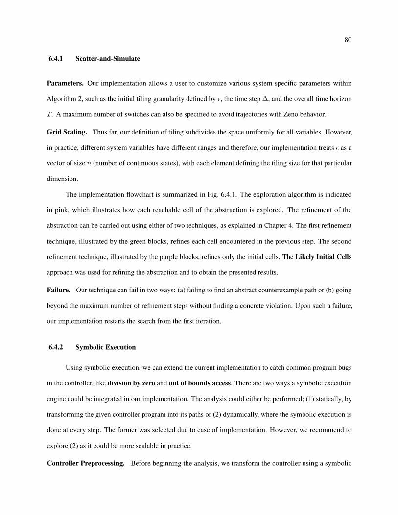
80

6.4.1 Scatter-and-Simulate

Parameters. Our implementation allows a user to customize various system specific parameters within

Algorithm 2, such as the initial tiling granularity defined by ε, the time step ∆, and the overall time horizon

T . A maximum number of switches can also be specified to avoid trajectories with Zeno behavior.

Grid Scaling. Thus far, our definition of tiling subdivides the space uniformly for all variables. However,

in practice, different system variables have different ranges and therefore, our implementation treats ε as a

vector of size n (number of continuous states), with each element defining the tiling size for that particular

dimension.

The implementation flowchart is summarized in Fig. 6.4.1. The exploration algorithm is indicated

in pink, which illustrates how each reachable cell of the abstraction is explored. The refinement of the

abstraction can be carried out using either of two techniques, as explained in Chapter 4. The first refinement

technique, illustrated by the green blocks, refines each cell encountered in the previous step. The second

refinement technique, illustrated by the purple blocks, refines only the initial cells. The Likely Initial Cells

approach was used for refining the abstraction and to obtain the presented results.

Failure. Our technique can fail in two ways: (a) failing to find an abstract counterexample path or (b) going

beyond the maximum number of refinement steps without finding a concrete violation. Upon such a failure,

our implementation restarts the search from the first iteration.

6.4.2 Symbolic Execution

Using symbolic execution, we can extend the current implementation to catch common program bugs

in the controller, like division by zero and out of bounds access. There are two ways a symbolic execution

engine could be integrated in our implementation. The analysis could either be performed; (1) statically, by

transforming the given controller program into its paths or (2) dynamically, where the symbolic execution is

done at every step. The former was selected due to ease of implementation. However, we recommend to

explore (2) as it could be more scalable in practice.

Controller Preprocessing. Before beginning the analysis, we transform the controller using a symbolic

81

Figure 6.3: Algorithm

82

execution engine to a set of all possible control-flow paths in the controller. The paths are represented by

their associated path constraints and update functions. This enumeration is expensive and carried only once

for a given controller. Once pre-processed, a controller move involves checking the feasibility of each path

constraint and if feasible, computing the valuations of updated state and output. We use Z3 [44], an SMT

solver to check feasibility and compute a concrete satisfying assignment on the controller’s input (y, s). The

update function is then used to compute (s′,u). Multiple satisfying assignments can be obtained by adding

blocking constraints.

SymEx Tools. Several tools for symbolic execution of code exist, but most are research projects. We tried

two mature tools, KLEE [27] and Pathcrawler [162]. We preferred the latter, as KLEE uses bitvector theories

to model floating point numbers which endures a performance penalty when reasoning about floating point

numerical code. Pathcrawler uses ECLiPSe [151] as its constraint solver. During the time of experiments,

both Pathcrawler and Z3 did not support the floating points. Instead, theory of reals was used. Presently, both

support floating point arithmetic. Although Pathcrawler and Z3 provide for efficient linear constraint solving,

they limit the kind of non-linear constraints that can be handled (in the controller).

Constraint Blowup. The symbolic treatment of the controller code has benefits of being precise. But,

as in the case with similar methodologies, like bounded model checking, automatic test generation, and

more, it suffers from ‘constraint blowup’. Each controller move requires an ‘unrolling’ of the controller

in time, tracking the associated constraints. The constraints accumulate with each time step and become

very inefficient to solve. Even though SMT solvers are quite efficient, large constraints can make the entire

analysis unusable. We address this by providing an option of selecting the ‘history depth’. Once the given

depth is exceeded, the symbolic controller states are concretized, and the accumulated symbolic constraints

(history) are purged. This is done by selecting some representative concrete controller states instead of

maintaining complex symbolic representation of all reachable controller states. To clarify, it does not limit

the length of the abstract trajectories that can be discovered. For all the presented benchmarks, a depth of 1

was used.

Parallelization. In its current form, S3CAM is not parallelized, but it can be parallelized owing to the

83

independent nature of plant simulations. In fact, the earlier prototype presented in [165] was parallelized.

The reason can be partially attributed to the difficulty of threading in Python. In the future, we plan to explore

fine grained lazy approaches to make parallelization more efficient.

6.5 Evaluation and Comparison

We evaluated S3CAM on multiple benchmarks ranging from mathematical systems to representative

systems from industry. This included both dynamical systems and SDCS. As S3CAM can accept a black

box description of a system, for the case of SDCS we compared the results both with and without symbolic

execution.

There are not many falsification tools which can be directly compared to S3CAM/X. Most tools do not

accept black box descriptions or SDCS. We compare against uniform random testing and S-TaLiRo. We also

compared with dReal/dReach in our publication [165]. The tested version of dReach could not falsify most

of the benchmarks.

6.5.1 Setup

S-TaLiRo and S3CAM/X use randomized algorithms. To get consistent results, we run them 10 times

on each benchmark, and note down the number of times they can find a violating trajectory. As the tools are

best effort and use restarts, we use a 1hr timeout to indicate a failed run. For a quantitative comparison, we

also collect the avg. time taken. However, because the tools are prototypes and not optimized, the timings

should only be qualitatively assessed. Also, S3CAM can execute simulations in parallel while S-TaLiRo can

not 2 .

Random Testing. While comparing the tools, the performance of random testing is also noted. Using

a uniform random distribution on the search space, we collect 105 samples and use them to numerically

simulate the benchmark. The generated traces are then examined for being violations. The number of

violations found are tabulated alongside the tools’ performances. Note that, for some benchmarks, we used

random testing to find properties that ‘appeared’ hard to falsify. This can bias some benchmarks towards2 The recent versions of S-TaLiRo can compute in parallel.

84

properties which are hard to falsify using uniform random sampling. In the future, having a set of curated

benchmarks from industry can help alleviate this.

Note: Though S3CAM-X also implements S3CAM’s functionality, the results use two different

versions of S3CAM’s implementation. Hence, the two tables should not be compared directly for timing

performances.

Hardware Setup. All the computations were carried out on a machine with a 4 core Intel i7-2820QM

2.30GHz CPU (up to 3.40GHz) and 8GB RAM, running Ubuntu 12.04

6.6 Case Studies for S3CAM (Dynamical Systems)

We evaluated our method on a number of examples, ranging from academic models of nonlinear and

hybrid dynamical systems, to models representative of industrial control systems.

6.6.1 Mathematical Dynamical Systems

The first set of benchmarks includes well known examples of complex nonlinear systems such as the

Van der Pol oscillator [154], the Brusselator, and the Lorenz reactor [154].

Van der Pol Oscillator

The Van der Pol Oscillator is tested with µ = 5, with both the initial states ranging between x ∈

[−0.4, 0.4].

x1 = x2

x2 = µ(1− x21)x2 − x1

The safety properties are selected based on the difficulty to falsify them using random simulations. The

properties P1, P2, P3 have a time horizon = 1s and their unsafe set of states XP1f , XP2

f , XP3f are shown in

Fig. 6.4.

The last property P4 explicitly specifies the time bound, between which, the unsafe states must be

85

XP1f =

{x1 ∈ [−1,−0.7]x2 ∈ [−6.5− 5.8]

XP2f =

{x1 ∈ [−1,−0.7]x2 ∈ [−6.5− 5.5]

XP3f =

{x1 ∈ [−1,−0.7]x2 ∈ [−6.5− 5.6]

Figure 6.4: Unsafe states.

reached. To check this, we add time as another state with its evolution given by t = 1.

P4 =

x1 ∈ [−1,−0.7]

x2 ∈ [−6.5− 5.8]

t ∈ [2.5, 4.5]

Lorenz System

The Lorenz system σ = 10, ρ = 28, β = 2.6667 is described in Fig. 6.5. The time horizon of the

property was 10s.

x = σ(y − x)

y = x(ρ− z)− y

z = xy − βz

x ∈ [−2, 2]

y ∈ [−2, 2]

z ∈ [−2, 2]

Initial states.

x ∈ [2.5, 3]

y ∈ [0, 4]

z ∈ [−∞∞]

Unsafe states.

Figure 6.5: Lorenz System.

Brusselator

The Brusselator [14] models a type of autocatalytic reaction. We have used it with the parameters

a = 1 and b = 2.5 and checked the safety property for a time horizon of 10s.

86

x1 = 1 + ax21x2 − (b+ 1)x1

x2 = bx1 − ax21x2

x1 ∈ [0, 1]

x2 ∈ [1, 2]

Initial states.

x1 ∈ [2.3, 2.4]

x2 ∈ [1.2, 1.3]

Unsafe states.

Figure 6.6: Brusselator.

6.6.2 Hybrid Dynamical Systems

The second set of benchmarks contain hybrid dynamical systems: a 4 state model of a bouncing ball,

a variation (B.Ball+S.H.M.) with the ball bouncing on a simple harmonically oscillating platform, and a

constrained pendulum [158]. Again, these systems have no formal specification of an unsafe region. We use

random testing to synthesize challenging falsification goals by identifying ‘hard-to-reach’ regions.

The third set of benchmarks consists of a modified instance of navigation benchmark (NAV-30) [164],

derived from [61]. These benchmarks describe a particle moving through a 2D grid, with different affine

motion dynamics for each cell. The falsification problem is to determine if certain cells are reachable, given

the initial position and velocities of the particle.

Bouncing Ball

The bouncing ball hybrid automaton with the safety property is illustrated in Fig. 6.7.

Constrained Pendulum

The benchmark from [158] describes a simple pendulum, constrained using a pin with a parameterized

location xp ∈ [1, 1.5]. The presence of the pin results in hybrid dynamics. It introduces two dynamical

modes, one in which the pendulum is swinging unconstrained from the point of suspension and another in

which the pin becomes the point of suspension (Fig. 6.8).

87

Mode: `I : y ≥ 0

F :

x = vxy = vyvx = 0vy = −1

vy < 0 ∧ y ≤ 0→

v′y := −0.75vy

X0 :

x ∈ [−.1, .1]y ∈ [3, 4]vx ∈ [4, 10]vy ∈ [−5, 5]

Xf :

(x ∈ [330, 330.1]y ∈ [1, 1.1]

)

Figure 6.7: The hybrid automaton for a bouncing ball with initial set X0 and unsafe set Xf . The goal is tofind whether a trajectory starting from the initial set X0 can reach the specified unsafe set Xf within 40s.

Mode: ConstrainedI : θ ≤ π/18

F :

[θ = ω/(L− xp)ω = −g sin(θ)− 0.5ω

]

Mode: UnconstrainedI : θ ≥ π/18

F :

[θ = ω/Lω = −g sin(θ)− 0.5ω

]

θ ≤ π/18θ ≥ π/18

X0 :

θ ∈ [ 4π18, 5π18

]ω ∈ [−1, 1]xp ∈ [1, 1.5]

Xf :

(θ ∈ [0.0, 0.12]ω ∈ [1.2, 1.5]

)

Figure 6.8: Constrained pendulum.

88

Navigation Benchmarks

NAV benchmarks are state partitioned hybrid systems commonly used to evaluate verification/falsifica-

tion tools [61]. These benchmarks model a particle traveling on a 2 dimensional grid of cells, each dictating

a differing affine continuous dynamics. A transition is taken when the particle crosses over from one cell

to its neighbor. All instances of the benchmark designate an initial set of states and an error cell. To test

our approach we focus on the largest instance “NAV-30”, which has 625 discrete modes and about 2500

possible transitions between them. To make the falsification more challenging, the initial sets modified to

X0 : x ∈ [4, 5], y ∈ [21, 22], vx ∈ [−1, 1], vy ∈ [−1, 1]. We pick safety properties PP , PQ, PR, PS , as

described in Chapter 3.

6.6.3 Physical Systems

Glucose-Insulin Control with Artificial Pancreas(G-I)

This benchmark is based on work by Fisher [62] and describes an artificial pancreas controller to

maintain safe levels of plasma blood glucose (pbg) in type I diabetes patients. The insulin-glucose dynamics

are modeled using the Bergman minimal model [17]. The plant model uses an exponential glucose absorption

sub-model. Using data of 18 different subjects [18] we search for the scenario of hypoglycemia (i.e.,

pbg < 3.6 mmol/L). We incorporate an uncertainty interval for each of the patient parameters in our model.

We only report the result for the case (patient ID:1) where we found a violation.

Idle Speed Controller

When a car is stationary, but the engine is running, it is required for the engine speed to be maintained

at a certain reference value in the presence of external disturbances such as torque demand (τ`) (example,

due to the A/C system) and the clutch being operated. We use a simplified affine hybrid automaton model of

a closed-loop system containing a model of the engine and the powertrain, with a single control input: the

throttle plate angle. The controller uses Proportional + Integral (PI) control to maintain the engine speed to

800± 35rpm. The aim of the falsifier is to find a simulation trace in the closed-loop model which exceeds

this range for time-varying values of τ` ∈ [0, 5]Nm.

89

6.7 Case Studies for S3CAM-X (SDCS)

Table 6.1: Summary of benchmarks. Each benchmark mentions the sampling period of the controller τs andits description is split into constituent controller and plant. The controller is described by number of States,exogenous inputs (Ex. Ip), lines of code (LOC), symbolic paths in the (Paths) and time taken to generatethem (SymEx Time) in minutes. The plant is described by the language used to implement its model (Impl.),number of modes if its a hybrid automaton in Python (Py) or the number of blocks if its a Simulink R©(SM)model (Modes/Blocks), continuous states (C. States)

Benchmark τs(s) Controller Plant

States Ex. Ip LOC Paths SymEx Time Impl. Modes/Blocks C. States

SPI 1 0 1 13 3 0 Py 1 1Heater 0.2 4 0 59 26 0 Py 3 1Heat 0.5 3 0 37 312 1 Py 6 3DC Motor 0.02 1 1 29 3 0 Py 0 2FuzzyC 0.01 0 0 218 208 236 Py 0 3MRS 1 0 8 29 9 0 Py 0 4AFC 0.01 7 0 243 120 40 SM 170 12

The benchmarks used for grey box testing are summarized in Table 6.1. Against each system tested,

we mention its sampling period τs and the controller and plant characteristics. For the former, this includes

the number of states, exogenous inputs, lines of code, symbolic controller paths statically discovered by

Pathcrawler and the time taken to do so. The plant is characterized by the implementation language for the

simulator (Python or Simulink R©), the number of discrete modes if the plant is a hybrid system, otherwise the

number of Simulink R© blocks, and lastly, the number of continuous states. A detailed description for each of

the benchmark follows.

Heat Benchmarks

The heat benchmarks proposed in [61], describe a scenario where a limited number of heaters h are

being used to heat r rooms, where h < r. The control system can shuffle the heaters or turn them on/off in

order to maintain a comfortable temperature in all rooms. We are interested in finding scenarios where the

controller fails and the temperature of any room dips below a certain threshold. We choose the first instance

in the suite of heat benchmarks for case study; this instance has 3 rooms and 1 heater. The controller software

has 312 control-flow paths and 3 states tracking each room’s temperature. Correspondingly, the plant has 3

continuous states and 6 modes. Each mode is characterized by the heater’s location and it’s discrete state

90

(on/off). We try to falsify the property that temperature of the first room does not drop below 17.23◦C.

Interestingly, S3CAM-X performs comparably to S3CAM even though the control software has 312 paths.

Both tools are faster than S-TaLiRo and finish in a few seconds, where as S-TaLiRo requires a few minutes

for falsification.

Sampled Polarity Integrator System (SPI)

The SPI benchmark was used in [49] to highlight the difficulty faced by Markov-chain Monte-Carlo

based random testing techniques, and optimization-guided techniques such as RRT-REX and S-TaLiRo.

The system has an exogenous input w, and a single continuous state x which after every τs = 1 seconds

gets reset to either -1, 0, or 1 if the input w < 0, w = 0 or w > 0 respectively. We split this system into

a plant and a controller, where the controller computes u = −1, 0, 1 based upon its exogenous input w as

u = sign(w). The continuous state of the plant evolves as x = u. We then check the three properties

P1 : x < 20, P2 : x < 50 and P3 : x < 150 for time horizons 50, 200, and 500 respectively. For all

properties S3CAM takes only a few seconds. S3CAM-X takes a bit longer due to constraint solving, but,

S-TaLiRo takes significantly longer and times out for P3. Similar difficulty is faced by RRT-Rex [49]. This

example brings out the difference in our iterative approach when compared to directed random search.

Heater

The heater system introduced in Chapter 5 consists of a room, and a heater controlled by a thermostat.

The heater has 3 operating modes; off, regular heating, and fast heating. It can be switched between modes

by the thermostat in order to reach and maintain a comfortable temperature in the room. Specifically, the

thermostat is designed to sense the room temperature after every τs = 0.2s and maintain a temperature of

around 70◦F . It also has built-in logic to prevent chattering, i.e., avoiding rapid switching of the heater

between modes. The heater is modeled as a hybrid system with linear dynamics, with 1 continuous state and

three modes. The thermostat’s software controller has 26 control-flow paths with 4 states which keep track of

recent mode switchings. The property we seek to falsify is that the room-temperature TF is always greater

than 52◦F . We are able to find the falsification trace, which upon investigation indicates the failure of the

chatter-prevention logic in a very narrow range of possible initial settings for the ambient room temperature

91

(approx.) TF0 ∈ [69.9, 70.0]. Though all tools find the falsification in less than half a minute, S3CAM-X is

an order of magnitude faster than both S3CAM and S-TaLiRo (for this benchmark).

DC Motor

This example illustrates the search for errors in the presence of controller disturbance. The DC motor

is a linear continuous system with armature current i and angular velocity θ. It is controlled by a PI controller

with saturation which results in 3 control-flow paths. The bounded additive disturbance in the controller

induces error in the sensed plant outputs. We parameterize the disturbance as a piecewise constant signal. We

wish the system to never enter the following region of the state-space: i ∈ [1, 1.2], θ ∈ [10, 11]. We choose

this set by design; it is designed to be very hard to reach using random simulations. S3CAM-X can, however,

find a falsification, demonstrating the effectiveness of symbolic execution in finding a sequence of inputs that

lead to a violation. In comparison, S-TaLiRo and our previous technique S3CAM fail to find a violation.

Fuzzy Control of Inverted Pendulum (FuzzyC)

Rule based controllers, such as ones implemented using fuzzy logic, are an interesting challenge for

symbolic execution based analyses as they typically have a large number of control-flow paths. We consider

an example from [131], where the controller tries to stabilize a nonlinear inverted pendulum balanced on a

cart using a 5× 5 rule matrix. The C code 3 has 218 lines describing 208 control-flow paths. The controller

is stateless and computes the actuation force by classifying the current plant state (θ and θ) and selecting

a corresponding control output from a lookup table. The safety property defines bounds on states, which

when exceeded, indicate undesirable transients or possible unstable behaviors. S-TaLiRo finds a falsifying

trajectory faster than S3CAM-X, but not as fast as S3CAM. This result is nevertheless encouraging as it

shows the ability of S3CAM-X to analyze a large number of control-flow paths and yet be successful at

finding a falsifying trajectory.

Mode-Specific Reference Selection (MRS)

These are a set of 3 benchmarks from [45, 49]. The benchmarks represent distinctive features from

proprietary models of automotive controllers, and they highlight issues faced by optimization-guided methods.3 http://www2.ece.ohio-state.edu/~passino/fuzzycontrol.html

92

The systems have simple nonlinear dynamics but complex combinatorial Boolean logic over 8 exogenous

inputs. To make the system amenable to S3CAM-X, we split the discrete nonlinear dynamics into a plant,

and the rest (linear combinatorial logic) becomes the controller. The controller remains the same across the

3 benchmarks, but the plant varies. The mode selection logic is now part of the controller which takes in

8 inputs w1, . . . , w8, where each wi ∈ [0, 100] and computes u. The 3 plants have discrete-time nonlinear

dynamics where the evolution is governed by x+ = f(x, u), where fi(x, u) comprises of polynomials of

up to degree 3 and trigonometric functions in x. The falsification can only be found in the mode which

is triggered when∧i∈[1..4]w2i(t) > 90 ∧ w2i−1(t) < 10. The probability of triggering the mode is thus a

meager 10−8. Such a combinatorial search is not amenable to sampling-based searches, and both S-TaLiRo

and S3CAM fail. On the other hand, S3CAM-X can falsify the property in under a minute.

Powertrain Control Benchmark (AFC)

We use the most complex version of the abstract fuel control system benchmark (AFC) presented

in [89]. It represents a complex closed loop control system modeling a plant with hybrid dynamics controlled

by a PI controller. The original benchmark has both the plant and the controller implemented in Simulink R©

(Fig. 6.7). To test it using our approach, we use Embedded Coder R© to generate C code for the controller block,

which is then hand-tuned to satisfy controller interface requirements. Due to the observability requirement,

the plant model is modified by simplifying the variable transport delay block to a first order filter. The

property checked is a modified form of the ‘Worst-case excursions in the normal mode’ property in [89], i.e.,

we try to falsify µ >= 0.02 while t ∈ [0, 1.0]. The search is over the original parameters: pedal frequency,

pedal amplitude and engine speed. Both S3CAM-X and S3CAM take longer than S-TaLiRo to find the

falsification due to the inefficient Matlab R© interface, as explained below.

6.8 Results

We split the discussion of the results into two sections: black box testing and grey box testing.

93

Figure 6.9: Simulink diagram of the powertrain benchmark

94

Table 6.2: All times are in minutes. Mean falsification times (Tavg) were computed on only the successfulruns out of 10 total runs. Unsuccessful runs indicate a timeout (≥ 1hr). Columns at the left summarizethe benchmarks, with the number of continuous states(S), inputs(I), parameters(P) and discrete Modes (‘-’implies a purely continuous system). Random simulations (100,000) and scatter-and-simulate use 4 threads,while S-Taliro used a single thread.

Benchmark S I P Modes Prop. Random Testing S-Taliro Scatter-SimNum. T Succ. Tavg Succ. TavgVio. (mins.) Runs (mins.) Runs (mins.)

P1 0 10.2 10 0.9 10 0.4Van der 2 0 0 - P2 21 41.9 10 11.8 10 2.9Pol [154] P3 19 26.4 10 2.5 10 1.6

P4 11 42.5 8 18.4 10 6.6Lorenz [154] 4 0 0 - P 36 132 3 20.6 10 3.1Brusselator 2 0 0 - P 429 22 10 1.1 10 0.2B.Ball [164] 4 0 0 1 P1 3 20 1 11.0 10 6.5B.Ball P1 13k 202 10 0.5 10 0.4+ 5 0 0 1 P2 3k 202 10 1.4 10 0.4S.H.M. P3 378 202 10 6.3 10 0.4Pendulum [158] 3 0 1 2 P1 0 6.6 10 4.7 10 4.7

P2 0 25 10 5.2 10 1.2PP 1 200 3 24.9 10 5.0

Nav.30 4 0 0 625 PQ 7 200 1 48.1 10 5.5[61, 164] PR 1 200 10 23.2 10 17.5

PS 108 495 3 33.2 10 20.1Idle Speed [30] 9 2 0 4 P 70 262 2 7.3 10 7.6MPC [88] 3 0 0 69 P 1 5.6 10 0.5 10 0.6G-I [17, 18, 62, 164] 4 0 2 2 P 1 30 10 5.0 10 4.0

95

6.8.1 Black Box Testing (Dynamical Systems)

The performance comparison of the tools is tabulated in Table 6.2. S3CAM was able to find a

falsification in every run, whereas S-TaLiRo failed in some instances. As stated earlier, the times taken

should not be directly compared. The S3CAM version (implemented in Matlab R©) was parallelized and used

4 threads, which gave it a substantial performance boost (verified by a 2X speedup for the bouncing ball

benchmark). This was in contrast with S-TaLiRo’s single threaded implementation. Qualitatively, S3CAM’s

performance is comparable, if not superior to S-TaLiRo. This may be attributed to S-TaLiRo’s use of global

search on robustness functions, which can be overly dependant on a good distance metric. In comparison,

S3CAM is relatively insensitive to distance metrics.

Comparing to random testing, we note that S3CAM can successfully find falsifications where 105

random simulations are unable to find any.

Scalability. Our approach scales successfully to some systems with as many as 14 state variables and in

some cases systems with hundreds of modes. In general, S3CAM succeeds because of

• relatively inexpensive simulations which can be easily computed in parallel, and

• multiple shooting, which is an efficient way to break down the complexity of the problem, specially

in the presence of highly non-linear trajectories.

6.8.2 Grey Box Testing (SDCS Systems)

As before, we compare S3CAM-X (S3CAM + SymEx) in Table 6.3 against S-TaLiRo. We also

compare its performance with black box testing without using SymEx, noted as S3CAM in the table. The

black box testing accesses the entire composed SDCS as a SIM function. We also provide the performance of

random testing using 100, 000 simulations (on most benchmarks except for AFC). Additionally S3CAM-X,

S-TaLiRo and random testing were executed using a single thread. If all 10 runs time out, we mention TO as

the time taken and 0 as the number of successful runs.

In summary, symbolic execution being an expensive operation, increases the overall time taken for the

search. This is evident when comparing the performance of S3CAM and S3CAM-X. At the same time, it

96

Table 6.3: Current tool S3CAMX, compared with S-Taliro and our previous tool S3CAM. All processeswere run as single threaded. All times are in minutes unless mentioned as seconds(s).

Benchmark Time Horizon Random Testing S-Taliro S3CAM S3CAMX

T (s) Num. Vio T Num. Succ Tavg Num. Succ Tavg Num. Succ Tavg

SPI(P1) 50 348/100k 17.5 10 0.36 10 0.01 10 0.22SPI(P2) 200 33 /100k 60.9 10 19.59 10 0.03 10 1.31SPI(P3) 500 0 /100k 154.4 0 TO 10 0.08 10 8.39Heater 2 47 /100k 3.9 10 0.48 10 0.22 10 0.06Heat 10 156/100k 39.0 10 11.78 10 0.06 10 0.16DC Motor 1 0 /100k 45.0 0 TO 0 TO 10 0.63FuzzyC 0.1 6 /100k 10.1 10 0.27 10 0.03 10 1.59MRS 1 2 0 /100k 0.6 0 TO 0 TO 10 0.18MRS 2 2 0 /100k 0.4 0 TO 0 TO 10 0.11MRS 3 2 0 /100k 0.4 0 TO 0 TO 10 0.43AFC 12 1 /100 238.7 10 0.25 10 16.15 10 13.45

97

also finds a falsification where S3CAM without SymEx completely fails. As noted from the benchmarks, this

happens in cases where the control program has non-robust or marginally robust paths (corner cases, which

are hard-to-cover behaviors using a uniform random distribution) leading to the violation. This is overcome

by SymEx as it does an exhaustive coverage of all possible control paths for a given set of plant states. It is

also not dependant on a distribution for sampling, unlike S3CAM. These cases are found in the DC Motor

and MRS benchmarks. When this is not the case, and the controller paths leading to the violation can be

covered using uniform random sampling alone, SymEx adds a performance penalty. This is evident by the

benchmarks: SPI, Heat and FuzzyC.

6.9 Concluding Remarks and Future Extensions

To conclude, we presented the tool S3CAM, which implements the approaches in the thesis. It also

provides a test bed to experiment with additional ideas. We now discuss a few extensions which can improve

the tool’s performance.

• Optimizations: The present implementation of S3CAM is in Python. A re-implementation in C /C++

can provide an immediate performance boost.

• Compositional Testing: S3CAM can be easily extended to compositionally reason over systems

composed of multiple copies of the plants. For example, systems with non-communicating multiple

agents, like satellites. Furthermore, we need to explore compositional reasoning when the plants are

different and communicate with each other.

• Incorporating Heuristics from AI: The numerical exploration of the plant can be improved by

using more sophisticated searches like A∗. Additionally, pattern databases can provide clever ways

to build the abstraction.

• Resource Bounded Exploration: In practice, it is critical that a tool works with the given set of

resources. Instead of terminating unexpectedly, it should be able to work with bounded memory. In

the future, we would like to modify the abstraction search to respect resource constraints by using

98

bounded memory algorithms.

• Integration of Symbolic Execution: We would like to integrate symbolic execution in a dynamical

fashion. To explain, the present implementation statically computes the symbolic paths of the

controller. A dynamic approach, which computes the symbolic states in every iteration can be more

scalable.

Chapter 7

Relational Modeling for Falsification

In Chapter 4, we analyzed systems by restricting ourselves to their black box semantics. This enabled

us to reason about the state-space reachability of the system without a direct analysis of its structure. Using a

coarse abstraction which we searched on-the-fly, we could observe the local dynamics as required. This gave

us an efficient procedure to find abstract counter-examples. However, to concretize the counter-examples, a

‘closer look’ or refinement of the abstraction is required. The grid based state-space abstraction was refined

by splitting the relevant cells (abstract states) into smaller ones. As noted previously, due to the curse of

dimensionality, such a uniform splitting is an expensive operation, and can not scale to higher dimensions.

In this chapter, we further our exploration of trajectory segment based methods; and explore an

alternative approach to overcome the explosion in abstract states. Instead of selectively refining the abstraction,

we compute a model of the black box system and use bounded model checking to find a concrete counter-

example in the model 1 . We then use this counter-example to guide the search towards a counter-example in

the original system.

More specifically, we use regression to quantitatively estimate the discovered relations, which were

witnessed by trajectory segments, by affine maps. These maps approximate locally observed behaviors,

which are incorporated into the sampled reachability graph as edge annotations. The resulting graph or the

Piece-Wise Affine (PWA) relational model can be interpreted as an infinite state discrete transition system

and model checked for time bounded safety properties. A counter-example if found, can indicate the presence

of a violation in the system.1 Due to modeling errors, this might not be reproducible in the original black-box system.

100

Towards the end of the chapter, we discuss extensions to data driven approaches (instead of simulator

driven), where instead of a simulator, a fixed set of data is provided as the behavioral description of the

system. Using a combination of relational modeling, and program analysis we outline the future work for

falsifying properties of SDCS.

7.1 Overview

We now briefly describe the approach. Given a numerical simulator SIM and an initial abstraction

defined by a quantization function Qε and a time step ∆, we use scatter-and-simulate (parameterized by

number of samples n as described in Chapter 4) to explore the abstract graphH(∆). The result is a graph G,

which has a finite number of abstract states C (or cells) and edges (C,C ′) iff C ∆ C ′.

Instead of using a CEGAR like loop (as in Chapter 4), we use the generated trajectory segments to

learn quantitative models describing the local behavior of the system. These models are defined by a set of

relations R ⊆ X × X for each edge of the reachability graph.

C

C ′

xi

x′i

πi

(a)

C C ′

R(C,C′) : {x′ ∈ Ax + b + δ}

(b)

Figure 7.1: (a) Trajectory segments πi are used to compute the relation R(C,C′) that annotates the edge in (b).R(C,C′) : {x′ ∈ Ax + b + δ} is an interval affine relation defined by an affine map (matrix A and vector b)and an error interval (vector of intervals δ).

Recall that each edge (C,C ′) of the graph G denotes an observed trajectory segment between the

respective cells. The graph abstraction G only states that there exists a state x ∈ C from which the system

can evolve to a future state x′ ∈ C ′. To increase the precision we iteratively refined the abstraction by

state splitting. Instead, we now propose an ‘enrichment’ GR of G by computing a set of local relations

R(C,C′)(x,x′) for every edge (C,C ′), which non-deterministically describe relations between x ∈ C and

x′ ∈ C ′. This is illustrated in Fig. 7.1 (compare with Fig. 4.3).

101

The enriched graph GR captures the underlying local forward dynamics describing the evolution of the

system in each abstract state. We represent the dynamics using an affine model with an interval error. Such

a model can either be approximated using learning methods or computed as a sound (over) approximation

using reachability set computation methods. Because we assume black box semantics, we only present the

former. Using regression analysis on the start and end states of the witnessed trajectory segments between

two cells, we compute an approximate discrete map along with an error estimate. Moreover, using the

simulation function SIM, additional trajectory segments (or data) can be generated if required. The data can

be separated into a training set and testing set to compute the map and the error respectively. The latter case

can be explored if the symbolic dynamics of the system are known. A tool like FLOW* [32] can be used to

find the reachable set map.

Observe that GR, a directed reachability graph, is rich enough to search for concrete behaviors in the

system. We call it a time parameterized PWA relational abstraction. It can be interpreted as an infinite state

discrete transition system, and we can use off-the-shelf bounded model checkers to find concrete violations

of a given safety property, and even other temporal properties. We now discuss the background required to

present our ideas.

7.2 Background

In this section, we present the basics of relational abstractions and fundamentals of regression analysis.

7.2.1 Relational Abstraction

For general hybrid dynamical systems, algorithmic ways for computing analytical solutions do not

exist. Discretization (along with suitable abstractions) is often employed to transform the systems into a

discrete transition system. Relational abstractions is one such idea, which abstracts continuous dynamics

by discrete relations using appropriate reachability invariants. Both time independent and time dependent

relations have been proposed; the former captures all reachable states over all time, whereas, the latter

explicitly includes time by relating reachable states to time. Thus it can prove timing properties whereas,

time independent relational abstractions can not. In both cases, the resulting abstractions can be interpreted

102

as discrete transition systems and can be analyzed using model checkers. We briefly discuss these two types

of abstractions.

Timeless Relational Abstraction

Relational abstractions for hybrid systems were proposed in [149]. For a hybrid automaton model,

they can summarize the continuous dynamics of each mode using a binary relation over continuous states.

The resulting relations are timeless (independent) and hence valid for all time as long as the mode invariant

is satisfied. The relations take the general form of R(x,x′) ./ 0, where ./ represents one of the relational

operators =,≥,≤, <,>. For example, an abstraction that captures the monotonicity with respect to time for

the differential equation x = 2 is x′ > x. The abstraction capturing the relation between the set of ODEs:

x = 2, y = 5, is 5(x′ − x) = 2(y′ − y).

Such relation summaries, discretize the continuous evolution of a given system into an infinite state

transition system, in which safety properties can be verified using k-induction, or falsified using bounded

model checkers. The relationalization procedure involves finding suitable invariants in a chosen abstract

domain, such as affine abstractions, eigen abstractions or box abstractions [149]. For this, different techniques

like template based invariant generation [36, 75] can be used.

Timed and Time-Aware Relational Abstractions

As the above discussed relations are timeless, we cannot reason over the timing properties of the original

system. Moreover, they are not suitable for time-triggered systems. Timed relational abstractions [166]

and time-aware relational abstractions [123] were proposed to overcome these shortcomings by explicitly

including time in the relations. In addition, both can be more precise than their timeless counterpart, but

unlike it, assume continuous affine dynamics.

To analyze time-triggered systems like an SDCS modeled by an affine hybrid automata 2 , timed

relational abstractions can be computed directly from the solutions of the underlying affine ODEs. Recall that

the solution of an affine ODE x = Ax can be represented using the matrix exponential as x(t) = etAx(0).

This gives us the timed relation x′ = etAx. Clearly, the relation is non-linear with respect to time. However,2 An affine hybrid automata is restricted to the ODEs, resets and guards being affine.

103

for the case of SDCS with a fixed sampling time period, we obtain linear relations in x. We demonstrated the

usefulness of timed relational abstractions for the case of linear systems in [166], and now incorporate the

idea to discretize black box dynamical systems.

Similar to timeless relational abstractions, time-aware relational abstractions [123] construct binary

relations between the current state x of the system and any future reachable state x′. The difference lies with

the latter also constructing relations between the current time t and any future time t′. This is achieved by a

case by case analysis of the eigen structure of the matrix A (of an affine ODE). Separate abstractions are used

for the case of linear systems with constant rate, real eigen values and complex eigenvalues.

7.2.2 Learning Dynamics using Simple Linear Regression

Regression Analysis

In statistics, regression is the problem of finding a predictor, which can suitably predict the relationship

between the given set of observed input x and output y vectors. In other words, assuming that y depends

on x, regression strategies find either a parameterized or a non-parameterized prediction function to explain

the dependence. We now discuss simple linear regression, which is parametric in nature and searches for an

affine predictor. It is also called ordinary least squares.

Ordinary Least Squares (OLS)

Let the data set be comprised of N input and output pairs (x, y), where x ∈ Rn and y ∈ R. If N > n,

which is the case in the current context of finding the best fit, the problem is over-determined; there are

more equations than unknowns. Hence, a single affine function cannot be found which satisfies the equation

∀i ∈ {1 . . . N}.yi = aTxi+ b. Instead, we need to find the ‘best’ choice for a and b. This is formally defined

using a loss function. For the case of simple linear regression or OLS, the loss function is the sum of squares

of the errors in prediction. The task is then to determine the vector of coefficients a and an offset constant b,

such that the least square error of the affine predictor is minimized for the given data set.

argmina,b

N∑i=1

(yi − (aTxi + b)

)2(7.1)

104

To ease the presentation, we can rewrite the above as a homogeneous expression by augmenting x by

x =

x1

and replacing a and b by the vector ab =

ab

. The equation 7.1 now becomes

argminab

N∑i=1

(yi − abT xi)2

The solution of OLS can be analytically computed as

Ab = (XTX)−1XTy

where X is the matrix representing the horizontal stacking of all x. The details can be found in several texts

on learning and statistics [67].

Given a time invariant dynamical system x′ = SIM(x,∆), where x ∈ Rn we can use OLS to

approximate its trajectories at fixed time step ∆ by a discrete map x′ = Ax + b, where A =

aT1...

aTn

and

b =

b1

...

bn

. This map is a global relational model for the system. The data set for the regression is a set of

pairs {(x,x′)|x′ = SIM(x,∆)} and can be generated on demand. Another set can be generated to compute

the error δ as an interval of vectors, where each element is an interval δi ∈ [δmin, δmax].

Affine maps are poor approximations for arbitrary non-linear functions. Hence, we use a collection of

affine maps to approximate the local behaviors (in state-space) of the system SIM. This results in a piece wise

approximation, as described in the next section.

7.2.3 Piecewise Affine (PWA) Transition System

We define the PWA transition system as a transition system (ref. Sec. 2.2.2) ρ : 〈L,V, T , l0,Θ〉 where

each transition τ ∈ T , is associated with a transition relation of the form

ρτ (v, v′) ⊆ {(v, fτ (v)) | gτ (v) ∧ g′τ (fτ (v))}

105

where fτ is an affine map relating the states and gτ , g′τ are affine guards (pre and post conditions) on the

states. The assertion on the initial states Θ is also affine.

We can now use a PWA transition system ρ to approximate the behavior of a hybrid dynamical system

S defined by a simulator SIMS3 . Each transition of ρ represents a discrete time step ∆. Let the state-space

of S be given by x ∈ X n, then the states of ρ are also given by x ∈ X n. The affine guard predicates gτ are

given by a conjunction of hyper-planes and hence can be represented in matrix form as a polyhedron (defined

by m constraints) in the state-space

g : Cx− d ≤ 0

where C is an m× n matrix and d is a vector of length m. The affine maps fτ can be represented in matrix

form as f : x 7→ Ax + b. To make fτ ‘richer’, we incorporate an error term δ which is defined by a vector

of intervals [δmin, δmax]. Hence,

f : x 7→ Ax + b + δ

defines a set valued relation of the form R : {(x,x′) | x′ ∈ fτ (x)}.

We now formalize the PWA affine transition system for a dynamical system.

Definition 7.2.1 (PWA Transition System) Given a hybrid dynamical system over a state-spaceX n, a PWA

transition system ρ is given by the tuple 〈L,x, T , l0,Θ〉, where τ ∈ T are affine transition relations and

Θ is an affine predicate over x and the states x ∈ X n. The transition relation is then defined by T with n

transition relations as follows

T =

g1(x) ∧ g′1(x′) =⇒ x′ ∈ f1(x)

. . .

gn(x) ∧ g′n(x′) =⇒ x′ ∈ fn(x)

(7.2)

where fi : x 7→ Aix + bi + δi, gi(x) : Cix− di ≤ 0, g′i(x′) : C ′ix

′ − d′i ≤ 0 and x′ denotes the next

state of the system.

A PWA model is deterministic, iff for every state x ∈ X n, a unique guarded affine map is satisfied

and all errors δ are singletons. However, in practice such a case rarely exists. A PWA model will be usually3 Due to fτ being restricted to an affine form, we can only approximate general hybrid systems.

106

non-deterministic, both due to multiple choice of transition relations and the reachable states at the kth time

step (or after k∆ units of time) being a set. Abusing the notation, we denote the set of states reachable in a

single step in ρ by x′ = ρ(x).

A PWA transition system is complete, iff for every state x ∈ X n, there exists at least one satisfied

transition relation T . If this is not the case, the system can deadlock, with no further executions. This usually

results from incorrect modeling of SDCS, and from here on, we do not consider such cases.

7.3 Relational Modeling

We now describe how relational models can be computed for a given black box system by enriching

the abstract reachability graph obtained by scatter-and-simulate. We first formalize the notion of an enriched

graph, and then show how they can be interpreted as a PWA transition system using k-relational modeling.

7.3.1 Abstract Enriched Graph

The existential abstraction relation in Chapter 4 was defined as follows:

Ct C ′ ⇐⇒ ∃x ∈ C. ∃x′ ∈ C ′. x t

x′

The abstract relation t can be enriched by incorporating the affine relation between x and x′. For an arbitrary

dynamical system, such a relation can be rarely represented using an exact affine map. This is due to the

presence of non-linear and hybrid behaviors. But, an affine map can always be estimated with an error.

If the system dynamics are completely specified in the form of a white box model, we can use first

order approximations to find the affine expressions for the relations. Using a tool like FLOW*, we can obtain

sound over-approximate affine maps of the form Ax+ [bl,bh], where [bl,bh] denotes the interval of vectors,

such that, every element bi of the vector b is contained in the respective scalar interval bi ∈ [bli, bhi ].

For the case of black box systems, such a sound approximation is not possible. Instead, we rely on a

statistical method like simple linear regression to estimate the affine map f : Ax + b. We then estimate the

error δ and generalize f to an interval affine map as before f : Ax + b + δ. Finally, we get an abstraction

107

with the below relation

Cf C ′ ⇐⇒ ∃x ∈ C. ∃x′ ∈ C ′. x′ ∈ Ax + b± δ.

However, in the presence of complex non-linear behavior, using a single affine map can lead to a poor

approximation. To increase the precision, one can use more than one affine map. Let us denote this set as

R(C,C′) (ref. Sec. 7.1).

R(C,C′)(x,x′) : {fi | ∃x ∈ C. ∃x′ ∈ C ′. x′ ∈ fi(x)}

G GREnrich using

Regression

(OLS)

Figure 7.2: Using OLS, GR is computed by determining the appropriate R(C,C′) for each edge of G.

As shown in Fig. 7.2, we use OLS to compute an enrichment of the abstraction graph G. For every

edge (C,C ′) ∈ edges(G), the set of relations R(C,C′)(x,x′) is computed. The semantics of the enriched

edge are clearly non-deterministic. Form a state x ∈ C, any fi ∈ R(C,C′) can be taken as long as x′ ∈ C’ is

satisfied. This interpretation results in an infinite state transition system. We now detail the construction of

the set R(C,C′) using k-relational modeling.

7.3.2 k - Relational Modeling

C C ′

C ′′1

C ′′2

k = 0 k = 1 k = 2

Figure 7.3: Nodes/Cells of G shown along with increasing values of k.

108

Given a G, when computing the set of relations for an edge R, we consider only the set of abstract

states reachable at a specific time step. Intuitively, one might consider the states reachable in one time step ∆.

However, such a process can be generalized by looking at the states reachable at 0∆, 1∆, . . . , k∆ time steps.

Using Fig. 7.3, we illustrate this notion. To compute R(C,C′), we split the data set D(C,C ′) consisting

of trajectory segments (of time lengths k∆) as follows. We observe the local behavior of the system by noting

the evolution of the system S from a state x(t) ∈ C for a time length dependant on k. For

• k = 0: we observe all trajectory segments of length ∆.

• k = 1: we observe trajectory segments of length ∆, which satisfy x(t+ ∆) ∈ C ′.

• k = 2: we observe trajectory segments of length 2∆, and split them in two sets (a) and (b) on the

basis of the cells reached at time (t+ ∆) and (t+ 2∆).

(a) x(t+ ∆) ∈ C ′ ∧ x(t+ 2∆) ∈ C ′′1

(b) x(t+ ∆) ∈ C ′ ∧ x(t+ 2∆) ∈ C ′′2

• k = n: we observe trajectory segments of length n∆, and split them in to multiple sets on the basis

of the cells reached at time (t+ ∆), (t+ 2∆), . . . , (t+ n∆).

k-relational modeling can be understood as a heuristic, which uses the underlying abstraction to

differentiate behaviors of the system which ‘diverge’ (or are revealed to be ‘distinct’ at a future time). Such a

heuristic can be useful in increasing the precision of the learnt affine maps. We now formalize this notion for

k = 0, 1, and n and illustrate using examples.

0-Relational Model

When k = 0, the 0-relational model is a PWA transition system which only defines the evolution of

states x, and does not specify the reachable cell. The guard predicates of the relations are defined over cells:

gi(x) : x ∈ Ci while g′i(x′) : True.

We use regression to estimate the dynamics for the outgoing trajectory segments form a cell C. Hence,

the data set D for the regression includes all trajectory segments beginning from the same cell

D = {πt|start(πt) ∈ C}.

109

C

x0

x′0

x1

x′1

x2

x′2

π1

π2

π3

t = 0 t = ∆

T ≡ g1(x) : x ∈ C =⇒ A1x+ b1 + δ1

Figure 7.4: All the trajectory segments will be used to construct the model; D = {π1, π2, π3}.

110

This includes trajectory segments ending in different cells, as shown in Fig. 7.4. For N cells, this results in a

ρ with N transition relations.

T =

g1(x) : x ∈ C1 =⇒ A1x + b1 + δ1

. . .

gn(x) : x ∈ Cn =⇒ Anx + bn + δn

Note that this can be quite imprecise when the cells are big, containing regions of state-space with

complex dynamics. This is true for both non-linear systems and hybrid dynamical system, where a cell can

contain two or more modes with differing continuous dynamics.

1-Relational Model

C

C ′1

C ′2

x0

x1

x2

x′0

x′1

x′2

π1

π2

π3

t = 0 t = ∆

T =

{g1(x) : x ∈ C ∧ g′1(x) : x ∈ C′1 =⇒ A1x+ b1 + δ1g2(x) : x ∈ C ∧ g′2(x) : x ∈ C′2 =⇒ A2x+ b2 + δ2

Figure 7.5: The data gets split into two sets D1 = {π1, π2} and D2 = {π3} and two relations: R(C,C′1) andR(C,C′2), each with one affine map, are constructed.

To improve the preciseness of learnt dynamics, we include the reachability relation in the regression.

For every relation C t C ′, the data set D is comprised only of trajectory segments πt which start and end in

the same set of cells.

D = {πt|start(πt) ∈ C ∧ end(πt) ∈ C ′}.

111

For N edges in G, 1-relationalization results in a ρ with N transition relations.

Fig. 7.5 illustrates the k = 1 refinement of the case shown in Fig. 7.4. The data set D is split into

two data sets D1 = {π1, π2} and D2 = {π3}, using which, two relations are constructed. The resulting

1-relational model is at least as precise as the corresponding 0-relational model.

k-Relational Model

C

C ′1 C ′′1

C ′′2

x0

x1

x′0

x′1x′′0

x′′1

π1

π2

t = 0 t = ∆ t = 2∆

T =

{g1(x) : x ∈ C ∧ g′1(x) : x ∈ C′1 =⇒ A1x+ b1 + δ1g1(x) : x ∈ C ∧ g′1(x) : x ∈ C′1 =⇒ A2x+ b2 + δ2

Figure 7.6: The k = 2 refinement further splits the data set D1 into two sets D11 = {π1} and D12 = {π2}and R(C,C′1) now has two affine maps, non-deterministically defining the system behavior.

Finally, we generalize the relational models to k-relational PWA models. A k-relational model is

constructed by using k length connected segmented trajectories. A segmented trajectory Sπ is connected iff

its cost COST(Sπ) = 0.

Two Sπ : 〈πt1 , . . . , πtk〉 and S′π :⟨π′t1 , . . . , π

′tk

⟩are similar if their trajectory segments have the same

sequence of cell traversals 〈C1, C2, . . . , Ck〉, i.e.

∀i ∈ {1 . . . k}.start(πti) ∈ Ci ∧ start(π′ti) ∈ Ci ∧ end(πti) ∈ Ci+1 ∧ end(π′ti) ∈ Ci+1

For every cell C in the reachability graph, we construct a data set D by collecting πti , such that they

are the first segment of k length connected and similar segmented trajectories.

112

Fig. 7.6 illustrates the k = 2 refinement on Fig. 7.5.

7.4 Bounded Model Checking Black Box Systems

We now describe the entire procedure in three steps.

(1) Given a black box system S specified by SIMS , we use scatter-and-simulate with (∆-length) trajectory

segments to sample a finite reachability graphH(∆).

(2) Using regression, we enrich the graph relations and annotate the edges with the estimated affine

maps.

(3) Interpreting the directed reachability graph as a transition system, we use a bounded model checker

to find fixed length violations to safety properties.

7.5 An Example: Van der Pol Oscillator

We now describe the above using the Van der Pol oscillator benchmark presented in Sec. 6.6.1.

Simulations generated using uniformly random samples are shown in Fig. 7.5. We want to check the property

P3, indicated by the red box, given the initial set indicated by the green box. The abstraction is defined by

Q0.2(x), which results in an evenly gridded state-space, where each cell is of size 0.2×0.2 units. Scatter-and-

simulate is then used to construct the abstract graph G, using 2 samples per cell and the time step ∆ = 0.1s.

The complete process follows.

(1) Abstract Consider an implicit abstraction induced by the quantization function Qε(x). The corre-

sponding reachability graphH(∆) (with time step ∆) is given by⟨C, ∆ , C0, Cu

⟩.

(2) Discover: Using scatter-and-simulate, enumerate a finite number of cells (vertices) and the relations

(edges) of the graphH(∆). Associate the set of generated trajectory segments with their respective

originating cells using a map D : C 7→ {π|start(π) ∈ C}. The discovered abstraction is show in

Fig. 7.5. As mentioned, red cells are unsafe and green cells are initial cells.

113

(3) Relationalize For each cell C, perform regression analysis on the respective set of trajectory

segments D(C), and compute a set of affine relations RC,C′(x,x′) between x ∈ C and x′ ∈ C ′ s.t.,

edge(C,C ′) ∈ H(∆). Annotate each edge in the graphH(∆) with the respective relation.

Fig. 7.5 shows the cells and the trajectory segments which are part of the data sets constructed using

the 1-relational modeling. Against each cell, its unique identifier (integer co-ordinate) is mentioned.

Finally, Fig. 7.5 and Table 7.1 show the enriched graph GR with its transition relations. Note that

self loops result when an observed trajectory segment has its start and end states in the same cell.

(4) Model Check The graphH(∆) can now be viewed as a transition system 〈C,x, T , C0,X0〉, where

C ∈ vertices(H(∆)) and x ∈ X . A transition τ ∈ T is of the form 〈C,C ′, ρτ 〉, where ρτ (x,x′) ⊆

{R(C,C′)(x,x′)|(C,C ′) ∈ edge(H(∆))}.

(5) Check Counter-example The infinite state (but finite location) transition system can be model

checked to find a concrete counter-example, which if exists, can indicate the existence of a similar

trace in the original black-box system S. The latter check is carried out as before, using the

numerical simulation function SIM. For the given example, the model checker is unable to find a

counter-example.

7.5.1 Search Parameters

The search parameters for S3CAM-R include the parameters of S3CAM: N , ε and ∆. Additionally,

they also include the maximum error budget δmax for OLS and the maximum length of segmented trajectory

for building k-relational models.

We have already discussed the effects of N , ε and ∆ on S3CAM’s performance. However, they also

have an effect on relational modeling. A finer grid with small cells produces more accurate models than

a coarser grid with large cells. Similarly, small time length trajectory segments result in more accurate

modeling.

Maximum Model Error (δmax) . Given a δmax, we keep increasing k during the k-relational modeling

114

Figure 7.7: Van der Pol: continuous trajectories. Red and green boxes indicate unsafe and initial sets.

Figure 7.8: The discovered abstractionH(0.1). Red cells are unsafe cells and green cells are initial cells.

115

Figure 7.9: Cells and trajectory segments used by 1-relational modeling.

Figure 7.10: Enriched graph GR. The affine maps f for the transition relations are show in Table 7.1.

116

Table 7.1: PWA model computed using OLS. The affine model for each edge (C,C ′) in the graph Fig. 7.5 isgiven by x′ ∈ Ax+ b+ δ, where δ is a vector of intervals.

C C ′ A b δ

(0, -1) (0, -1)[

0.99 0.12−0.12 1.63

] [00

] [[0, 0][0, 0]

](0, -1) (0, -2)

[0.99 0.12−0.10 1.63

] [00

] [[0, 0][0, 0]

](0, -2) (0, -2)

[0.99 0.12−0.09 1.63

] [00

] [[0, 0][0, 0]

](0, -2) (0, -4)

[0.99 0.12−0.07 1.62

] [00

] [[0, 0][0, 0]

](0, -9) (-1, -15)

[0.99 0.12−0.09 1.61

] [0

−0.04

] [[0, 0]

[0, 0.01]

](-1, -15) (-3, -24)

[0.95 0.12−1.29 1.47

] [−0.01−0.41

] [[0, 0]

[0, 0.01]

](-3, -24) (-4, -29)

[1.11 −0.17−1.71 0.66

] [−1.07−3.31

] [[−0.04, 0.04][−0.07, 0.09]

](-4, -29) (-4, -29)

[0.99 0.01−0.41 1.02

] [0

−0.28

] [[0, 0][0, 0]

](-1, -10) (-2, -16)

[0.97 0.12−0.71 1.56

] [0

−0.11

] [[0, 0]

[0, 0.01]

](-1, -10) (-2, -15)

[0.97 0.12−0.70 1.58

] [0

−0.08

] [[0, 0]

[0, 0.01]

](-2, -16) (-3, -23)

[0.92 0.12−1.84 1.39

] [−0.02−0.73

] [[0, 0][0, 0]

](-3, -23) (-5, -29)

[3.14 −0.81−0.96 0.23

] [−3.13−4.99

] [[−0.04, 0.03][−0.03, 0.04]

](-2, -15) (-3, -22)

[0.93 0.12−1.75 1.40

] [−0.02−0.68

] [[0, 0][0, 0]

](-3, -22) (-5, -29)

[3.08 −0.72−1.69 0.40

] [−2.77−4.57

] [[−0.02, 0.02][−0.01, 0.02]

]

117

process till δi ≤ δmax is satisfied. A kmax is introduced to bound the longest segmented trajectory which can

be considered.

7.5.2 Reasons for Failure

The approach can fail to find a counter-example, even when it exists, in one of three ways.

• S3CAM Fails No abstract counter-example is found by S3CAM. We can remedy it by increasing

search budgets and/or restarting.

• BMC Fails An abstract counter-example is found, but the BMC fails to find a concrete counter-

example in the PWA relational model. The failure can be attributed to either (a) a spurious abstract

counter-examples or (b) a poorly estimated model. The former can be addressed by restarting but

the latter requires that the maximum model error δmax be decreased.

• Inaccurate PWA Modeling An abstract counter-example is found, and it is successfully concretized

in the PWA relational model by the BMC. However, it is not reproducible in the black box system.

This happens when the PWA relational model is not precise enough.

7.6 Implementation and Evaluation

The implementation was prototyped as S3CAM-R, an extension to our previously mentioned tool

S3CAM (Chapter 6). OLS regression routines were used from Scikit-learn [132], a Python module for

machine learning. SAL [146] with Yices2 [51] was the model checker and the SMT solver.

We used S3CAM to discover the abstraction graph G, which was then trimmed of the nodes which did

not contribute to the error search (nodes from which error nodes were not reachable). In our experiments we

used 1-relational modeling to create the transition system fromG. Using SAL, we checked for the given safety

property. If a concrete trace was obtained from the BMC, it was further checked for validity by simulating

using SIM to see if it was indeed an error trace. If not, 100 samples from its associated abstract state was

sampled to check the presence of a counter-example in it neighborhood. This can be further extended by

obtaining different discrete sequences or discrete trace sequences from the model checker.

118

We tabulate our preliminary evaluation in Table 7.2. We used few of the benchmarks described in

Chapter 6, including the Van der Pol oscillator, Brusselator, Lorenz attractor and the Navigation benchmark.

As before, we ran S3CAM-R 10 times with different seeds and averaged the results. We tabulate both the

total time taken and the time taken by SAL to compute the counter-example and compare against a newer

implementation of S3CAM. Note that different abstraction parameters are used for S3CAM and S3CAM-R,

due to the differences in which they operate.

Table 7.2: Avg. timings for benchmarks. The BMC column lists time taken by the BMC engine. The totaltime in seconds (rounded off to an integer) is noted under S3CAM-R and S3CAM. TO signifies time > 5hr,after which the search was killed.

Benchmark BMC S3CAM-R S3CAM

Van der Pol (P3) <1 130 24Brusselator <1 4 2Lorenz <1 122 35Nav (PP ) 5862 11520 603Nav (PQ) 2216 6847 546Nav (PR) - TO 2003Nav (PS) - TO 2100Bouncing Ball - TO 450

The results show promise, but clearly S3CAM performs better. Also, S3CAM-R timed out on some

benchmarks like Nav PR, Nav PS and the bouncing ball. However, we need to explore more benchmarks to

be conclusive. S3CAM-R’s performance can be explained by the difficulty in finding a good abstraction Qε,

which needs to be fine enough, to obtain good prediction models but coarse enough, to be manageable by the

current SMT solvers. Specifically, to obtain a good quality counter-example from the model checker (and

avoid false positives), the transition system should be created from models with high accuracy, for which a

finer abstraction is required. However, the exploration of a finer abstraction is exponentially more complex

and results in a much bigger transition system, which the current state of the art bounded model checkers

(which use SMT solvers) can not handle under reasonable resources.

119

7.7 Conclusion and Future Work

We have presented another methodology to find falsifications in black box dynamical systems. Com-

bining the ideas from abstraction based search (Chapter 4), with our previous relational abstractions [166],

we proposed k-relational modeling to compute richer abstractions. Simple linear regression can be used to

estimate the local dynamics of the trajectory segments and compute PWA relational models which can be

interpreted as a transition system. These can then be checked for safety violations using an off-the-shelf

bounded model checker. Finally, we implemented the ideas as a tool S3CAM-R and demonstrated its

performance on a few examples.

7.7.1 Improvements

The approach seems promising as it avoids an expensive refinement step. But, before it can be applied

to more complex systems, we need to overcome its shortcomings. As a future extension, we are investigating

ideas to improve the performance of the underlying three main sub-processes, namely, abstraction, modeling,

and BMC. We detail these below.

(1) Abstraction The abstract domain we have used, has been confined to the interval or rectangular

domain. Such a domain is very coarse when compared to more general polyhedral domains, using

which, we can gain better precision. Due to polyhedral domains being computational expensive,

their integration in S3CAM needs to be explored thoroughly.

(2) Modeling We have used k-relational modeling to increase the precision of the enriched abstractions,

however, there are several other refinement strategies that remain to be explored. This includes

refining the abstract states by using guard predicates (similar to predicate abstraction), using non-

linear templates in parametric regression to compute more precise quadratic relations, and using an

adaptive time step instead of a fixed one to address the non-linearities due to a long time horizon.

(3) Model Checking As of now, we use SMT solvers to search for concrete counter-examples. Although

they are very efficient, owing to extensive engineering effort, reachability of transition systems result-

120

ing from dynamical systems remains a difficult problem. As the time horizon of the safety property

increases, the possible combinations of discrete transitions increase exponentially. Hence, to find a

counterexample which is a sequence of discrete transitions over a ‘long’ time horizon is not tractable

for most, but the simplest of dynamical systems. Instead, we can use linear programming solvers,

by enumerating each path in the graph GR. Note that the constraints are all linear (conjunctions)

along an abstract path. However, in the worst case, the number of paths in a graph can be of the

order n! where n is the number of vertices of a graph. Hence, this will not be feasible, unless, we

can prioritize paths by using a triage process similar to one used by S3CAM and using a budget on

the maximum number of paths.

Another approach to address the issue would be to use an adaptive time discretization technique,

where relations over both shorter and longer time steps are computed, and the SMT solver can

‘select’ the time step precise enough to find a counter-example.

(4) SMT Solvers One major impediment to our approach is the fact that SMT solvers use the theory

of reals with exact precision. This is important for verification approaches, but can be relaxed for

the problem of falsification. An SMT solver which uses approximate reasoning but returns robust

counter-examples will be as useful, and perhaps more efficient.

7.7.2 Data Driven Analysis

Finally, we would like to mention that our approach is ‘simulation’ driven. It can be easily modified to

be ‘data driven’, by working with a fixed set of data. Given a data set, we then need to automatically find a

good abstraction and a high fidelity PWA transition system using which, we can summarize the black box

hybrid dynamical system. Apart from model checking the transition system, one can extend it to the analysis

of SDCS. More specifically, by combining the transition system model of a plant with the control software, a

model checker like CBMC [100] can be used to do a closed loop symbolic analysis of the SDCS. This can be

an alternative to S3CAM-X.

Chapter 8

Conclusions

In conclusion, we presented techniques for finding safety violations in cyber-physical systems (CPS).

We put forth a combination of symbolic and numerical analysis to automatically analyze sampled-data control

systems. The numerical analysis is specialized for the exploration of behaviors of a dynamical system.

Moreover, it requires only the numerical simulation function as the definition for the system and makes

minimal assumptions. On the other hand, the symbolic analysis is software specific and rigorously explores

all paths of the software. Using the two together results in a highly applicable and scalable approach.

We demonstrated the approach by implementing it as a tool: S3CAM, which we tested on several

benchmarks. S3CAM’s performance is shown to be as good, if not better, than the currently available tools.

It is able to find falsifications even when the other tools fail.

There are several aspects of our approach which can be improved upon; and there are many more

unexplored avenues which can enable the widespread acceptance of automatic falsification methods. We

discuss them below.

MTL Properties

We have focused on falsifying simple safety properties. Many important properties of systems are

temporal in nature, and expressible in temporal logics like LTL/MTL/STL. We can extend our techniques to

handle temporal properties by using monitors [116–118]. However, done naively, it might not yield acceptable

performance in practice. Hence, efficient methods must be explored.

Compositional Analysis

122

In practice, systems are often specified as compositions of sub-systems. Engineering and development

tools like Simulink R©, encourage ‘block’ based compositional methodologies. A complex system block is

created by specifying simpler sub-system blocks and defining their interactions. A similar notion is true

for software, where natural slices or partitions in the program can exist. Program slicing has been explored

in [3, 43, 98, 153, 155, 159]. Exploring compositional analyses can increase our applicability; and also give us

efficient procedures to analyze large systems by decomposing them into smaller ones.

Input Output Relationalization

A limitation of the current numerical exploration of the plant is the requirement of state observability.

This is often restrictive in practice. An exploration into the space of input output relational abstractions seems

natural. We would like to explore reduced order modeling techniques [143,150] and relational abstractions of

the plants in order to obtain simpler models. This can tremendously improve the scalability of our current

approaches by reducing the state-space dimensionality. PWA relational abstractions constructed through

machine learning techniques (Chapter 7), highlight our first steps in this direction.

Specialization to Control Software

Using an off-the-shelf symbolic executor for analyzing the control software has its limitations. The

symbolic executor is engineered for general purpose software and misses out on the optimizations which

are specific to the domain of control software. Also, it does not provide domain specific functionality, like

dimensional analysis [129], which can be very useful. Another extension would be to introduce relaxations,

like concolic executions, which can improve the scalability of the overall analysis.

Tool Improvements

Finally, we would like to improve our tool S3CAM. We would like to address implementation aspects

like, memory and run time optimizations, extension to various input formats used in the industry and automatic

parameter selection.

Bibliography

[1] Houssam Abbas, Georgios Fainekos, Sriram Sankaranarayanan, Franjo Ivancic, and Aarti Gupta.Probabilistic temporal logic falsification of cyber-physical systems. Trans. on Embedded ComputingSystems (TECS), 12(2s):95, 2012.

[2] Houssam Abbas, Andrew Winn, Georgios Fainekos, and A Agung Julius. Functional gradient descentmethod for metric temporal logic specifications. In 2014 American Control Conference, pages 2312–2317. IEEE, 2014.

[3] Hiralal Agrawal and Joseph R Horgan. Dynamic program slicing. In ACM SIGPLAN Notices,volume 25, pages 246–256. ACM, 1990.

[4] Rajeev Alur. Formal verification of hybrid systems. In Embedded Software (EMSOFT), 2011Proceedings of the International Conference on, pages 273–278. IEEE, 2011.

[5] Rajeev Alur. Principles of cyber-physical systems. MIT Press, 2015.

[6] Rajeev Alur, Costas Courcoubetis, Nicolas Halbwachs, P.-H. Ho Thomas A. Henzinger, XavierNicollin, Alfredo Olivero, Joseph Sifakis, and Sergio Yovine. The algorithmic analysis of hybridsystems. Theoretical computer science, 138(1):3–34, 1995.

[7] Rajeev Alur, Thao Dang, and Franjo Ivancic. Counter-example guided predicate abstraction of hybridsystems. In TACAS, volume 2619 of LNCS, pages 208–223. Springer, 2003.

[8] Rajeev Alur, Thomas A. Henzinger, G. Lafferriere, and George Pappas. Discrete abstractions of hybridsystems. Proc. of IEEE, 88(7):971–984, 2000.

[9] Rajeev Alur, Thomas A Henzinger, Gerardo Lafferriere, and George J Pappas. Discrete abstractions ofhybrid systems. Proceedings of the IEEE, 88(7):971–984, 2000.

[10] Yashwanth Annpureddy, Che Liu, Georgios Fainekos, and Sriram Sankaranarayanan. S-taliro: A toolfor temporal logic falsification for hybrid systems. Springer, 2011.

[11] Eugene Asarin, Thao Dang, and Antoine Girard. Hybridization methods for the analysis of nonlinearsystems. Acta Informatica, 43:451—476, 2007.

[12] Uri M Ascher, Robert MM Mattheij, and Robert D Russell. Numerical solution of boundary valueproblems for ordinary differential equations, volume 13. Siam, 1994.

[13] J-P Aubin, John Lygeros, Marc Quincampoix, Shankar Sastry, and Nicolas Seube. Impulse differentialinclusions: a viability approach to hybrid systems. Automatic Control, IEEE Transactions on, 47(1):2–20, 2002.

124

[14] Shaun Ault and Erik Holmgreen. Dynamics of the brusselator. Math 715 Projects (Autumn 2002),page 2, 2003.

[15] Gerd Behrmann, Alexandre David, and Kim G. Larsen. A tutorial on UPPAAL. In SFM-RT 200 (Revised Lectures), volume 3185 of LNCS, pages 200–237. Springer Verlag, 2004.

[16] Luca Benvenuti, Davide Bresolin, Alberto Casagrande, Pieter Collins, Alberto Ferrari, EmanueleMazzi, Alberto Sangiovanni-Vincentelli, and Riziano Villa. Reachability computation for hybridsystems with Ariadne. In Proc. the 17th IFAC World Congress, 2008.

[17] Richard N Bergman. Toward physiological understanding of glucose tolerance: minimal-modelapproach. Diabetes, 38(12):1512–1527, 1989.

[18] Richard N Bergman, Lawrence S Phillips, and Claudio Cobelli. Physiologic evaluation of factors con-trolling glucose tolerance in man: measurement of insulin sensitivity and beta-cell glucose sensitivityfrom the response to intravenous glucose. Journal of Clinical Investigation, 68(6):1456, 1981.

[19] Martin Berz and Kyoko Makino. Verified integration of odes and flows using differential algebraicmethods on high-order taylor models. Reliable Computing, 4(4):361–369, 1998.

[20] Martin Berz and Kyoko Makino. Performance of Taylor model methods for validated integration ofODEs. LNCS, 3732:65–74, 2005.

[21] John T Betts. Survey of numerical methods for trajectory optimization. Journal of guidance, control,and dynamics, 21(2):193–207, 1998.

[22] John T Betts. Practical methods for optimal control and estimation using nonlinear programming,volume 19. Siam, 2010.

[23] Amit Bhatia and Emilio Frazzoli. Incremental search methods for reachability analysis of continuousand hybrid systems. Proc. of HSCC, page 451–471, 2004.

[24] Hans Georg Bock and Karl-Josef Plitt. A multiple shooting algorithm for direct solution of optimalcontrol problems. 1983.

[25] M. Branicky, M. Curtiss, J. Levine, and S. Morgan. Sampling-based planning, control and verificationof hybrid systems. IEE Proc.-Control Theory Appl., 153(5):575–590, 2006.

[26] Michael S Branicky. Introduction to hybrid systems. In Handbook of Networked and EmbeddedControl Systems, pages 91–116. Springer, 2005.

[27] Cristian Cadar, Daniel Dunbar, and Dawson R Engler. Klee: Unassisted and automatic generation ofhigh-coverage tests for complex systems programs. In OSDI, volume 8, pages 209–224, 2008.

[28] Cristian Cadar, Patrice Godefroid, Sarfraz Khurshid, Corina S Pasareanu, Koushik Sen, NikolaiTillmann, and Willem Visser. Symbolic execution for software testing in practice: preliminaryassessment. In Proceedings of the 33rd International Conference on Software Engineering, pages1066–1071. ACM, 2011.

[29] Cristian Cadar and Koushik Sen. Symbolic execution for software testing: three decades later.Communications of the ACM, 56(2):82–90, 2013.

125

[30] Alberto Casagrande, Andrea Balluchi, Luca Benvenuti, Alberto Policriti, Tiziano Villa, andAL Sangiovanni-Vincentelli. A new algorithm for reachability analysis of hybrid automata. Technicalreport, Citeseer.

[31] Xin Chen, Erika Abrahám, and Sriram Sankaranarayanan. Taylor model flowpipe construction fornon-linear hybrid systems. In Real-Time Systems Symposium (RTSS), pages 183–192. IEEE, 2012.

[32] Xin Chen, Erika Ábrahám, and Sriram Sankaranarayanan. Flow*: An analyzer for non-linear hybridsystems. In Computer Aided Verification, pages 258–263. Springer, 2013.

[33] Edmund Clarke, Ansgar Fehnker, Zhi Han, Bruce Krogh, Joël Ouaknine, Olaf Stursberg, and MichaelTheobald. Abstraction and counterexample-guided refinement in model checking of hybrid systems.International Journal of Foundations of Computer Science, 14(04):583–604, 2003.

[34] Edmund M. Clarke, Orna Grumberg, Somesh Jha, Yuan Lu, and Helmut Veith. Counterexample-guidedabstraction refinement for symbolic model checking. J. ACM, 50(5):752–794, 2003.

[35] Edmund M. Clarke, Orna Grumberg, and Doron A. Peled. Model Checking. MIT Press, 1999.

[36] Michael Colón, Sriram Sankaranarayanan, and Henny Sipma. Linear invariant generation usingnon-linear constraint solving. In CAV, volume 2725 of LNCS, pages 420–433. Springer, July 2003.

[37] P. Cousot and R. Cousot. Abstract interpretation: a unified lattice model for static analysis ofprograms by construction or approximation of fixpoints. In Conference Record of the Fourth AnnualACM SIGPLAN-SIGACT Symposium on Principles of Programming Languages, pages 238–252,Los Angeles, California, 1977. ACM Press, New York, NY.

[38] T. Dang, A. Donze, O. Maler, and N. Shalev. Sensitive state-space exploration. In Proc. of the 47thIEEE CDC, pages 4049–4054, Dec. 2008.

[39] Thao Dang, Alexandre Donzé, Oded Maler, and Noa Shalev. Sensitive state-space exploration. InDecision and Control, 2008. CDC 2008. 47th IEEE Conference on, pages 4049–4054. IEEE, 2008.

[40] Thao Dang, Oded Maler, and Romain Testylier. Accurate hybridization of nonlinear systems. InHSCC ’10, pages 11–20. ACM, 2010.

[41] Thao Dang and Tarik Nahhal. Coverage-guided test generation for continuous and hybrid systems.Formal Methods in System Design, 34(2):183–213, 2009.

[42] Thao Dang and Tarik Nahhal. Coverage-guided test generation for continuous and hybrid systems.Formal Methods in System Design, 34(2):183–213, 2009.

[43] Andrea De Lucia et al. Program slicing: Methods and applications. In scam, pages 144–151, 2001.

[44] Leonardo De Moura and Nikolaj Bjørner. Z3: An efficient smt solver. In Tools and Algorithms forthe Construction and Analysis of Systems, pages 337–340. Springer, 2008.

[45] Jyotirmoy Deshmukh, Xiaoqing Jin, James Kapinski, and Oded Maler. Stochastic local searchfor falsification of hybrid systems. In Automated Technology for Verification and Analysis, pages500–517. Springer, 2015.

[46] A. Donzé and O. Maler. Robust satisfaction of temporal logic over real-valued signals. In Proc.FORMATS, pages 92–106, 2010.

126

[47] Alexandre Donzé. Breach, a toolbox for verification and parameter synthesis of hybrid systems. InProc. CAV, pages 167–170, 2010.

[48] Alexandre Donzé and Oded Maler. Systematic simulation using sensitivity analysis. In HybridSystems: Computation and Control, pages 174–189. Springer, 2007.

[49] Tommaso Dreossi, Thao Dang, Alexandre Donzé, James Kapinski, Xiaoqing Jin, and Jyotirmoy VDeshmukh. Efficient guiding strategies for testing of temporal properties of hybrid systems. In NASAFormal Methods, pages 127–142. Springer, 2015.

[50] Parasara Sridhar Duggirala and Sayan Mitra. Abstraction refinement for stability. In Cyber-PhysicalSystems (ICCPS), 2011 IEEE/ACM International Conference on, pages 22–31. IEEE, 2011.

[51] Bruno Dutertre. Yices 2.2. In International Conference on Computer Aided Verification, pages737–744. Springer, 2014.

[52] Bruno Dutertre and Leonardo De Moura. The yices smt solver. Tool paper at http://yices. csl. sri.com/tool-paper. pdf, 2:2, 2006.

[53] Joel M. Esposito, Jongwoo Kim, and Vijay Kumar. Adaptive rrts for validating hybrid robotic controlsystems. In Workshop on Algorithmic Foundations of Robotics, pages 107–132, 2004.

[54] Joel M. Esposito, Jongwoo Kim, and Vijay Kumar. Adaptive RRTs for validating hybrid roboticcontrol systems. In Proceedings of the International Workshop on the Algorithmic Foundations ofRobotics, 2004.

[55] Joel M Esposito, Jongwoo Kim, and Vijay Kumar. Adaptive rrts for validating hybrid robotic controlsystems. In Algorithmic Foundations of Robotics VI, pages 107–121. Springer, 2005.

[56] Georgios Fainekos and George J. Pappas. Robustness of temporal logic specifications for continuous-time signals. Theoretical Computer Science, 410:4262–4291, 2009.

[57] Georgios E. Fainekos. Robustness of Temporal Logic Specifications. PhD thesis, Department ofComputer and Information Science, University of Pennsylvania, 2008.

[58] Georgios E. Fainekos, Antoine Girard, and George J. Pappas. Temporal logic verification usingsimulation. In FORMATS, volume 4202 of LNCS, pages 171–186. Springer, 2006.

[59] Georgios E Fainekos and George J Pappas. Robustness of temporal logic specifications for finite statesequences in metric spaces. Technical report, Technical Report MS-CIS-06-05, Dept. of CIS, Univ. ofPennsylvania, 2006.

[60] Georgios E Fainekos and George J Pappas. Robust sampling for mitl specifications. In FormalModeling and Analysis of Timed Systems, pages 147–162. Springer, 2007.

[61] Ansgar Fehnker and Franjo Ivancic. Benchmarks for hybrid systems verification. In HSCC, volume2993 of LNCS, pages 326–341. Springer, 2004.

[62] Michael E Fisher. A semiclosed-loop algorithm for the control of blood glucose levels in diabetics.Biomedical Engineering, IEEE Transactions on, 38(1):57–61, 1991.

[63] Martin Fränzle and Christian Herde. Hysat: An efficient proof engine for bounded model checking ofhybrid systems. Formal Methods in System Design, 30(3):179–198, 2007.

127

[64] Goran Frehse. PHAVer: Algorithmic Verification of Hybrid Systems Past HyTech. STTT, 10(3), June2008.

[65] Goran Frehse, Colas Le Guernic, Alexandre Donzé, Scott Cotton, Rajarshi Ray, Olivier Lebeltel,Rodolfo Ripado, Antoine Girard, Thao Dang, and Oded Maler. Spaceex: Scalable verification ofhybrid systems. In Computer Aided Verification, pages 379–395. Springer, 2011.

[66] Goran Frehse, Colas Le Guernic, Alexandre Donzé, Scott Cotton, Rajarshi Ray, Olivier Lebeltel,Rodolfo Ripado, Antoine Girard, Thao Dang, and Oded Maler. Spaceex: Scalable verification ofhybrid systems. In Proc. CAV, LNCS. Springer, 2011.

[67] Jerome Friedman, Trevor Hastie, and Robert Tibshirani. The elements of statistical learning, volume 1.Springer series in statistics Springer, Berlin, 2001.

[68] Sicun Gao, Soonho Kong, and Edmund M Clarke. dreal: An smt solver for nonlinear theories over thereals. In Automated Deduction–CADE-24, pages 208–214. Springer, 2013.

[69] Sicun Gao, Soonho Kong, and Edmund M Clarke. Satisfiability modulo odes. In Formal Methods inComputer-Aided Design (FMCAD), 2013, pages 105–112, 2013.

[70] Dimitra Giannakopoulou and Klaus Havelund. Automata-based verification of temporal properties onrunning programs. In Automated Software Engineering, 2001.(ASE 2001). Proceedings. 16th AnnualInternational Conference on, pages 412–416. IEEE, 2001.

[71] Antoine Girard. Reachability of uncertain linear systems using zonotopes. In HSCC, volume 3414 ofLNCS, pages 291–305. Springer, 2005.

[72] Antoine Girard and George J Pappas. Approximation metrics for discrete and continuous systems.2005.

[73] Rafal Goebel, Ricardo G Sanfelice, and Andrew R Teel. Hybrid Dynamical Systems: modeling,stability, and robustness. Princeton University Press, 2012.

[74] Colas Le Guernic and Antoine Girard. Reachability analysis of linear systems using support functions.Nonlinear Analysis: Hybrid Systems, 4(2):250 – 262, 2010.

[75] Sumit Gulwani and Ashish Tiwari. Constraint-based approach for hybrid systems. In CAV, volume5123 of LNCS, pages 190–203, 2008.

[76] Charles R Hargraves and SW Paris. Direct trajectory optimization using nonlinear programming andcollocation. Journal of Guidance, Control, and Dynamics, 10(4):338–342, 1987.

[77] Klaus Havelund and Grigore Rosu. Monitoring programs using rewriting. In Automated SoftwareEngineering, 2001.(ASE 2001). Proceedings. 16th Annual International Conference on, pages 135–143. IEEE, 2001.

[78] Klaus Havelund and Grigore Rosu. Synthesizing monitors for safety properties. In Tools andAlgorithms for the Construction and Analysis of Systems, pages 342–356. Springer, 2002.

[79] Thomas A. Henzinger. The theory of hybrid automata. In LICS’96, pages 278–292. IEEE, 1996.

[80] Thomas A Henzinger, Pei-Hsin Ho, and Howard Wong-Toi. Hytech: the next generation. In Real-TimeSystems Symposium, 1995. Proceedings., 16th IEEE, pages 56–65. IEEE, 1995.

128

[81] Thomas A. Henzinger, Pei-Hsin Ho, and Howard Wong-Toi. Algorithmic analysis of nonlinear hybridsystems. IEEE Transactions on Automatic Control, 43:540–554, 1998.

[82] Thomas A Henzinger, Peter W Kopke, Anuj Puri, and Pravin Varaiya. What’s decidable about hybridautomata? In Proceedings of the twenty-seventh annual ACM symposium on Theory of computing,pages 373–382. ACM, 1995.

[83] Thomas A Henzinger, Marius Minea, and Vinayak Prabhu. Assume-guarantee reasoning for hierarchi-cal hybrid systems. In International Workshop on Hybrid Systems: Computation and Control, pages275–290. Springer, 2001.

[84] Thomas A Henzinger, Shaz Qadeer, and Sriram K Rajamani. You assume, we guarantee: Methodol-ogy and case studies. In International Conference on Computer Aided Verification, pages 440–451.Springer, 1998.

[85] C. Herde, A. Eggers, and T. Franzle, M. Teige. Analysis of hybrid systems using HySAT. In ThirdInternational Conference on Systems, 2008. ICONS 08., pages 13–18. IEEE, 2008.

[86] Chieh Su Hsu. Cell-to-cell mapping: a method of global analysis for nonlinear systems, volume 64.Springer Science & Business Media, 2013.

[87] CS Hsu and RS Guttalu. An unravelling algorithm for global analysis of dynamical systems: anapplication of cell-to-cell mappings. Journal of Applied Mechanics, 47(4):940–948, 1980.

[88] Mike Huang, Hayato Nakada, Srinivas Polavarapu, Richard Choroszucha, Ken Butts, and Ilya Kol-manovsky. Towards combining nonlinear and predictive control of diesel engines. In AmericanControl Conference, 2013. Proceedings of the 2004, pages 2852–2859. IEEE, 2013.

[89] Xiaoqing Jin, Jyotirmoy V Deshmukh, James Kapinski, Koichi Ueda, and Ken Butts. Powertrain con-trol verification benchmark. In Proceedings of the 17th international conference on Hybrid systems:computation and control, pages 253–262. ACM, 2014.

[90] A Agung Julius, Georgios E Fainekos, Madhukar Anand, Insup Lee, and George J Pappas. Robusttest generation and coverage for hybrid systems. In Hybrid Systems: Computation and Control, pages329–342. Springer, 2007.

[91] Aditya Kanade, Rajeev Alur, Franjo Ivancic, S. Ramesh, Sriram Sankaranarayanan, and K.C. Sashid-har. Generating and analyzing symbolic traces of Simulink/Stateflow models. In Computer-aidedVerification (CAV), volume 5643 of LNCS, pages 430–445, 2009.

[92] Aditya Kanade, Rajeev Alur, Franjo Ivancic, S Ramesh, Sriram Sankaranarayanan, and KC Shashid-har. Generating and analyzing symbolic traces of simulink/stateflow models. In Computer AidedVerification, pages 430–445. Springer, 2009.

[93] Jim Kapinski, Bruce H. Krogh, Oded Maler, and Olaf Stursberg. On systematic simulation of opencontinuous systems. In HSCC, volume 2623 of LNCS, pages 283–297. Springer, 2003.

[94] Jongwoo Kim, Joel M. Esposito, and Vijay Kumar. An RRT-based algorithm for testing and validatingmulti-robot controllers. Technical report, DTIC Document, 2005.

[95] Jongwoo Kim, Joel M Esposito, and Vijay Kumar. An rrt-based algorithm for testing and validatingmulti-robot controllers. Technical report, DTIC Document, 2005.

129

[96] James C King. Symbolic execution and program testing. Communications of the ACM, 19(7):385–394,1976.

[97] Soonho Kong, Sicun Gao, Wei Chen, and Edmund Clarke. dreach: Delta-reachability analysis forhybrid systems. In Tools and Algorithms for the Construction and Analysis of Systems, 2015.

[98] Bogdan Korel and Janusz Laski. Dynamic program slicing. Information Processing Letters, 29(3):155–163, 1988.

[99] Ron Koymans. Specifying real-time properties with metric temporal logic. Real-time systems,2(4):255–299, 1990.

[100] Daniel Kroening and Michael Tautschnig. Cbmc–c bounded model checker. In InternationalConference on Tools and Algorithms for the Construction and Analysis of Systems, pages 389–391.Springer, 2014.

[101] Sebastian Kupferschmid, Jörg Hoffmann, Henning Dierks, and Gerd Behrmann. Adapting an AIplanning heuristic for directed model checking. In Proc. of SPIN, pages 35–52, 2006.

[102] Jan Kurátko and Stefan Ratschan. Combined global and local search for the falsification of hybridsystems. In International Conference on Formal Modeling and Analysis of Timed Systems, pages146–160. Springer, 2014.

[103] Jan Kuratko and Stefan Ratschan. Solving underdetermined boundary value problems by sequentialquadratic programming. arXiv preprint arXiv:1512.09078, 2015.

[104] Alexander B. Kurzhanski and Pravin Varaiya. Ellipsoidal techniques for reachability analysis. InHSCC, volume 1790 of LNCS, pages 202–214. Springer, 2000.

[105] A. A. Kurzhanskiy and P. Varaiya. Ellipsoidal toolbox. Technical Report UCB/EECS-2006-46, EECSDepartment, University of California, Berkeley, May 2006.

[106] Steven M LaValle. Rapidly-exploring random trees a new tool for path planning. 1998.

[107] Steven M LaValle and James J Kuffner Jr. Randomized kinodynamic planning. In Proc. ICRA,volume 1, pages 473–479. IEEE, 1999.

[108] Edward Ashford Lee and Sanjit Arunkumar Seshia. Introduction to embedded systems: Acyber-physical systems approach. Lee & Seshia, 2011.

[109] Flavio Lerda, James Kapinski, Edmund Clarke, and Bruce Krogh. Verification of supervisory controlsoftware using state proximity and merging. Hybrid Systems: Computation and Control, pages344–357, 2008.

[110] Flavio Lerda, James Kapinski, Hitashyam Maka, Edmund M Clarke, and Bruce H Krogh. Modelchecking in-the-loop: Finding counterexamples by systematic simulation. In American ControlConference, 2008, pages 2734–2740. IEEE, 2008.

[111] Jan Lunze and Françoise Lamnabhi-Lagarrigue. Handbook of hybrid systems control: theory, tools,applications. Cambridge University Press, 2009.

[112] John Lygeros. Lecture notes on hybrid systems. In Notes for an ENSIETA workshop, 2004.

130

[113] Rupak Majumdar, Indranil Saha, KC Shashidhar, and Zilong Wang. Clse: Closed-loop symbolicexecution. In NASA Formal Methods, pages 356–370. Springer, 2012.

[114] Oded Maler. A unified approach for studying discrete and continuous dynamical systems. In Decisionand Control, 1998. Proceedings of the 37th IEEE Conference on, volume 2, pages 2083–2088. IEEE,1998.

[115] Oded Maler. Algorithmic verification of continuous and hybrid systems. arXiv preprintarXiv:1403.0952, 2014.

[116] Oded Maler and Dejan Nickovic. Monitoring temporal properties of continuous signals. In FormalTechniques, Modelling and Analysis of Timed and Fault-Tolerant Systems, pages 152–166. Springer,2004.

[117] Oded Maler, Dejan Nickovic, and Amir Pnueli. From mitl to timed automata. In InternationalConference on Formal Modeling and Analysis of Timed Systems, pages 274–289. Springer, 2006.

[118] Oded Maler, Dejan Nickovic, and Amir Pnueli. Checking temporal properties of discrete, timed andcontinuous behaviors. In Pillars of computer science, pages 475–505. Springer, 2008.

[119] Zohar Manna and Amir Pnueli. Temporal Verification of Reactive Systems: Safety. Springer, NewYork, 1995.

[120] James D. Meiss. Differential Dynamical Systems. SIAM publishers, 2007.

[121] Ian Mitchell and Claire J Tomlin. Level set methods for computation in hybrid systems. In HybridSystems: Computation and Control, pages 310–323. Springer, 2000.

[122] Ian M Mitchell, Alexandre M Bayen, and Claire J Tomlin. A time-dependent hamilton-jacobiformulation of reachable sets for continuous dynamic games. Automatic Control, IEEE Transactionson, 50(7):947–957, 2005.

[123] Sergio Mover, Alessandro Cimatti, Ashish Tiwari, and Stefano Tonetta. Time-aware relational abstrac-tions for hybrid systems. In Embedded Software (EMSOFT), 2013 Proceedings of the InternationalConference on, pages 1–10. IEEE, 2013.

[124] Tadao Murata. Petri nets: Properties, analysis and applications. Proceedings of the IEEE, 77(4):541–580, 1989.

[125] Tarik Nahhal and Thao Dang. Test coverage for continuous and hybrid systems. In Computer AidedVerification, page 449–462, 2007.

[126] N. S. Nedialkov and M. von Mohrenschildt. Rigorous simulation of hybrid dynamic systems withsymbolic and interval methods. In Proc. of ACC, pages 140–146. IEEE, 2002.

[127] Truong Nghiem, Sriram Sankaranarayanan, Georgios Fainekos, Franjo Ivancic, Aarti Gupta, andGeorge J Pappas. Monte-carlo techniques for falsification of temporal properties of non-linear hybridsystems. In Proceedings of the 13th ACM international conference on Hybrid systems: computationand control, pages 211–220. ACM, 2010.

[128] Truong Nghiem, Sriram Sankaranarayanan, Georgios E. Fainekos, Franjo Ivancic, Aarti Gupta, andGeorge J. Pappas. Monte-carlo techniques for falsification of temporal properties of non-linear hybridsystems. In Hybrid Systems: Computation and Control, pages 211–220. ACM Press, 2010.

131

[129] Sam Owre, Indranil Saha, and Natarajan Shankar. Automatic dimensional analysis of cyber-physicalsystems. In International Symposium on Formal Methods, pages 356–371. Springer, 2012.

[130] Corina S Pasareanu, Matthew B Dwyer, and Michael Huth. Assume-guarantee model checking ofsoftware: A comparative case study. In International SPIN Workshop on Model Checking of Software,pages 168–183. Springer, 1999.

[131] Kevin M Passino, Stephen Yurkovich, and Michael Reinfrank. Fuzzy control, volume 42. Citeseer,1998.

[132] Fabian Pedregosa, Gaël Varoquaux, Alexandre Gramfort, Vincent Michel, Bertrand Thirion, OlivierGrisel, Mathieu Blondel, Peter Prettenhofer, Ron Weiss, Vincent Dubourg, et al. Scikit-learn: Machinelearning in python. Journal of Machine Learning Research, 12(Oct):2825–2830, 2011.

[133] James Lyle Peterson. Petri Net Theory and the Modeling of Systems. Prentice Hall, 1981.

[134] Erion Plaku, Lydia Kavraki, and Moshe Vardi. Falsification of LTL safety properties in hybrid systems.Proc. TACAS, page 368–382, 2009.

[135] André Platzer. Differential dynamic logic for hybrid systems. Journal of Automated Reasoning,41(2):143–189, 2008.

[136] André Platzer. Logical analysis of hybrid systems: proving theorems for complex dynamics. Springer,2010.

[137] André Platzer and Jan-David Quesel. Keymaera: A hybrid theorem prover for hybrid systems (systemdescription). In Automated Reasoning, pages 171–178. Springer, 2008.

[138] Pavithra Prabhakar and Miriam Garcia Soto. Abstraction based model-checking of stability of hybridsystems. In International Conference on Computer Aided Verification, pages 280–295. Springer,2013.

[139] Pavithra Prabhakar and Miriam García Soto. Counterexample guided abstraction refinement for stabilityanalysis. In International Conference on Computer Aided Verification, pages 495–512. Springer, 2016.

[140] Stephen Prajna and Ali Jadbabaie. Safety verification of hybrid systems using barrier certificates. InHybrid Systems: Computation and Control, pages 477–492. Springer, 2004.

[141] Stefan Ratschan and Zhikun She. Safety verification of hybrid systems by constraint propagationbased abstraction refinement. In HSCC, volume 3414 of LNCS, pages 573–589. Springer, 2005.

[142] Stefan Ratschan and Zhikun She. Safety verification of hybrid systems by constraint propagationbased abstraction refinement. In Hybrid Systems: Computation and Control, pages 573–589. Springer,2005.

[143] Michal Rewienski and Jacob White. A trajectory piecewise-linear approach to model order reduc-tion and fast simulation of nonlinear circuits and micromachined devices. IEEE Transactions oncomputer-aided design of integrated circuits and systems, 22(2):155–170, 2003.

[144] Julia Robinson. The collected works of Julia Robinson, volume 6. American Mathematical Soc.,1996.

132

[145] Hendrik Roehm, Jens Oehlerking, Matthias Woehrle, and Matthias Althoff. Reachset conformancetesting of hybrid automata. In Proceedings of the 19th International Conference on Hybrid Systems:Computation and Control, pages 277–286. ACM, 2016.

[146] John Rushby, Patrick Lincoln, Sam Owre, Natrajan Shankar, and Ashish Tiwari. Symbolic analysislaboratory (sal). Cf. http://www.csl.sri.com/projects/sal/.

[147] Sriram Sankaranarayanan, Thao Dang, and Franjo Ivancic. Symbolic model checking of hybridsystems using template polyhedra. In TACAS, volume 4963 of LNCS, pages 188–202. Springer, 2008.

[148] Sriram Sankaranarayanan, Henny Sipma, and Zohar Manna. Constructing invariants for hybrid systems.Formal Methods in System Design, 32(1):25–55, 2008.

[149] Sriram Sankaranarayanan and Ashish Tiwari. Relational abstractions for continuous and hybridsystems. In CAV, volume 6806 of LNCS, pages 686–702. Springer, 2011.

[150] Wilhelmus HA Schilders, Henk A Van der Vorst, and Joost Rommes. Model order reduction: theory,research aspects and applications, volume 13. Springer, 2008.

[151] Joachim Schimpf and Kish Shen. Ecl i ps e–from lp to clp. Theory and Practice of Logic Programming,12(1-2):127–156, 2012.

[152] Koushik Sen, Darko Marinov, and Gul Agha. CUTE: a concolic unit testing engine for C, volume 30.ACM, 2005.

[153] Josep Silva. A vocabulary of program slicing-based techniques. ACM computing surveys (CSUR),44(3):12, 2012.

[154] Steven H. Strogatz. Nonlinear Dynamics And Chaos. Perseus Books Group, 1 edition, 1994.

[155] Frank Tip. A survey of program slicing techniques. Journal of programming languages, 3(3):121–189,1995.

[156] Ashish Tiwari. Abstractions for hybrid systems. Formal Methods in Systems Design, 32:57–83, 2008.

[157] Ashish Tiwari. Hybridsal relational abstracter. In Computer Aided Verification, CAV’12, pages725–731. Springer-Verlag, 2012.

[158] Arjan J Van Der Schaft and Johannes Maria Schumacher. An introduction to hybrid dynamicalsystems, volume 251. Springer London, 2000.

[159] Mark Weiser. Program slicing. In Proceedings of the 5th international conference on Softwareengineering, pages 439–449. IEEE Press, 1981.

[160] Jan C Willems. The behavioral approach to modeling and control of dynamical systems. In AICHESYMPOSIUM SERIES, pages 97–108. New York; American Institute of Chemical Engineers; 1998,2002.

[161] Jan C Willems and Jan W Polderman. Introduction to mathematical systems theory: a behavioralapproach, volume 26. Springer Science & Business Media, 2013.

[162] Nicky Williams, Bruno Marre, Patricia Mouy, and Muriel Roger. Pathcrawler: Automatic generationof path tests by combining static and dynamic analysis. In Dependable Computing-EDCC 5, pages281–292. Springer, 2005.

133

[163] Aditya Zutshi, Sriram Sankaranarayanan, Jyotirmoy V Deshmukh, and Xiaoqing Jin. Symbolic-numeric reachability analysis of closed-loop control software. In Proceedings of the 19th InternationalConference on Hybrid Systems: Computation and Control, pages 135–144. ACM, 2016.

[164] Aditya Zutshi, Sriram Sankaranarayanan, Jyotirmoy V Deshmukh, and James Kapinski. A trajectorysplicing approach to concretizing counterexamples for hybrid systems. In IEEE Conf. on Decisionand Control (CDC). IEEE Press, 2013.

[165] Aditya Zutshi, Sriram Sankaranarayanan, Jyotirmoy V Deshmukh, and James Kapinski. Multipleshooting, cegar-based falsification for hybrid systems. In Proceedings of the 14th InternationalConference on Embedded Software, page 5. ACM, 2014.

[166] Aditya Zutshi, Sriram Sankaranarayanan, and Ashish Tiwari. Timed relational abstractions for sampleddata control systems. In Computer Aided Verification, pages 343–361. Springer, 2012.