Embed Size (px)
Citation preview

eeh power systemslaboratory
Nikolaos-Iason Avramiotis-Falireas
Re-Design of Automatically Activated
Control Reserves in the Swiss Power
System
Master ThesisPSL 1323
Department:EEH – Power Systems Laboratory, ETH Zurich
Examiner:Prof. Dr. Goran Andersson, ETH Zurich
Supervisors:Tobias Haring, ETH ZurichDr. Marek Zima, Swissgrid
Zurich, October 2013


ABSTRACT i
Abstract
This master thesis deals with the subject of re-designing the secondary fre-quency control reserves in the Swiss power system. The aim is to provide in-centives and to remove uneccessary barriers for additional market providersthat want to deliver secondary control. Aggregated devices are allowed toparticipate in the secondary control market in Switzerland, therefore thetarget is to design a new secondary control setup that takes into accountspecific properties of these potential providers, namely their fast rampingcapability, their energy limitations and their limitation in switching on/off,in order to respect duty-cycles.
Two issues that may give greater flexibility to providers and can enhancethe control performance were investigated in this thesis. First, the provisionof asymmetric secondary frequency control, and second the splitting of thecurrent secondary contol signal into a slow-changing and a volatile one. Forthe latter methodology, historical data of area control error and activatedsecondary control signal, provided by the Swiss Transmission System Op-erator, are analyzed and specific frequency components are identified. Thesecondary frequency control signal is splitted into a slow-changing compo-nent with a high energy content, and a volatile component that is consistedof the high frequencies, using filtering techniques. Several types of filters,as well as cutoff frequencies are compared in terms of energy, ramping andchanges in direction, using historical data. Then a second approach basedon an optimization setup is proposed, which effectively splits the secondarysignal by penalizing the energy requested from the volatile signal and theramping required by the slow-changing one. In this setup constraints for themaximum ramping deviation of the slow-changing signal and the maximumenergy deviation of the volatile signal are also formulated.
In order to evaluate the impact on the control performance of the pro-posed schemes time-domain simulations are performed. The probabilitydensity functions of the area control error are constructed, from which it isproven that the control performance of the proposed schemes is equal to thecurrent performance level, in almost all cases.
Finally, economic issues are taken into consideration and proposals forthe procurement and compensation methods for the adjusted control setupare formulated.
Key Words: Automatic Generation Control (AGC), fast AGC signal,slow-changing AGC signal, fast response resources.

ACKNOWLEDGEMENT ii
Acknowledgement
This master thesis was conducted in the ancillary services developmentgroup at Swissgrid ltd. and in the Power System Laboratory (PSL) atETH Zurich. I would like to thank all the people that contributed to thefulfillment of this thesis and especially:
• Dr. Marek Zima who gave me the opportunity to deal with this in-teresting area and for his valuable inputs and support throughout thisproject.
• Professor Dr. Goran Andersson for his support througout this masterprogram and for allowing me to deal with this interesting topic.
• Tobias Haring, PhD student at PSL, for our good collaboration andour fruitful discussions during the whole period of this thesis.
I would also like to thank all my friends in Switzerland and in Greecefor their continuous support and fun all over the years of my studies andespecially Eirini Andritsaki for her patience, support and encouragementduring the whole master programme and especially these last demandingmonths.
Finally I would like to express my graditude to my brother Odysseas andmy parents, Spyros and Angeliki, which without their total support and en-couragement nothing of all this would be possible.
Zurich, October 2013Nikolaos Iason Avramiotis Falireas

CONTENTS iii
Contents
1 Introduction 11.1 Motivation and Related Literature . . . . . . . . . . . . . . . 2
2 General Aspects of Secondary Frequency Control 52.1 Tasks and General Setup of Frequency Control . . . . . . . . 52.2 Primary Frequency Control . . . . . . . . . . . . . . . . . . . 62.3 Secondary Frequency Control . . . . . . . . . . . . . . . . . . 6
2.3.1 Current Status in Switzerland . . . . . . . . . . . . . . 72.4 Tertiary Frequency Control . . . . . . . . . . . . . . . . . . . 9
3 Analysis of Secondary Contol Historical Data 103.1 Construction and Observation of Power Imbalances . . . . . . 103.2 Discrete fourier Transform on the Power Imbalance Signal . . 12
3.2.1 Mathematical Formulation of DFT . . . . . . . . . . . 123.2.2 Application on Historical Data . . . . . . . . . . . . . 13
4 Asymmetric Secondary Control 164.1 Implications for the Providers . . . . . . . . . . . . . . . . . . 164.2 Implications for the TSO . . . . . . . . . . . . . . . . . . . . 17
4.2.1 Impact on Reserve Dimensioning . . . . . . . . . . . . 184.2.2 Adjustment of Participation factors . . . . . . . . . . 18
5 Adjustments of Control Concept 215.1 Filtering . . . . . . . . . . . . . . . . . . . . . . . . . . . . . . 21
5.1.1 Lowpass Filter Setup . . . . . . . . . . . . . . . . . . . 225.1.2 Highpass Filter Setup . . . . . . . . . . . . . . . . . . 305.1.3 Comparison of Filters . . . . . . . . . . . . . . . . . . 32
5.2 Optimizer . . . . . . . . . . . . . . . . . . . . . . . . . . . . . 38
6 Time Domain Simulations 486.1 Power System Modeling . . . . . . . . . . . . . . . . . . . . . 486.2 Time-Domain Simulations . . . . . . . . . . . . . . . . . . . . 53
6.2.1 First Scenario . . . . . . . . . . . . . . . . . . . . . . . 566.2.2 Second scenario . . . . . . . . . . . . . . . . . . . . . . 606.2.3 Discussion on Results . . . . . . . . . . . . . . . . . . 63
7 Adjustments of Procurement and Compensation 657.1 Current Practices for Procurement and Settlement . . . . . . 65
7.1.1 Procurement . . . . . . . . . . . . . . . . . . . . . . . 657.1.2 Compensation . . . . . . . . . . . . . . . . . . . . . . 667.1.3 Performance-Based Compensation . . . . . . . . . . . 67
7.2 Proposed Approach . . . . . . . . . . . . . . . . . . . . . . . . 717.2.1 Procurement . . . . . . . . . . . . . . . . . . . . . . . 71
LIST OF FIGURES iv
7.2.2 Settlement . . . . . . . . . . . . . . . . . . . . . . . . 73
8 Conclusions 76
A PDFs of ACE from Time-Domain Simulations 78A.1 Scenario 1 . . . . . . . . . . . . . . . . . . . . . . . . . . . . . 78A.2 Scenario 2 . . . . . . . . . . . . . . . . . . . . . . . . . . . . . 79
Literature 81
List of Figures
1 Frequency control concept [27] . . . . . . . . . . . . . . . . . 52 Control structure for AGC (∆ei = Error = ACEi = Area
Control Error for area i) [1] . . . . . . . . . . . . . . . . . . . 73 Test signal for LFC for Switzerland [37] . . . . . . . . . . . . 94 Secondary frequency control demand curve . . . . . . . . . . 115 Average secondary control curve for July 2012 . . . . . . . . . 116 Average secondary control curve for August 2012 . . . . . . . 117 Average secondary control curve for November 2012 . . . . . 128 Average secondary control curve for January 2013 . . . . . . 129 Frequency spectrum . . . . . . . . . . . . . . . . . . . . . . . 1410 Frequency spectrum over 3 month signal . . . . . . . . . . . . 1511 The original signal, the terms till 15 min and the dominant
frequency of 1-h . . . . . . . . . . . . . . . . . . . . . . . . . . 1512 Capacity allocation of generating unit and associated costs . 1713 Dimensioning of symmetric secondary: deficit rate 0.1% . . . 1914 Dimensioning of asymmetric secondary: deficit rate 0.05% for
positve and the same for negative . . . . . . . . . . . . . . . . 1915 Filtering of the output of PI controler and creating two con-
trol signals . . . . . . . . . . . . . . . . . . . . . . . . . . . . 2116 Filtering of the output of PI controler with a lowpass filter . 2217 Frequency response and taps’ weights of 201 order FIR filter . 2418 FIlter output, complement and intial signal . . . . . . . . . . 2519 Frequency response and taps’ weights of an 11-order FIR filter 2620 Filter output, complement and initial signal . . . . . . . . . . 2721 Frequency response and fIlter output 3rd order low-pass But-
terworth, complement and intial signal . . . . . . . . . . . . . 2822 Frequency response and filter output 3rd order low-pass Cheby-
shev type I, complement and intial signal . . . . . . . . . . . 2923 Frequency response and filter output Exponential Weighted
Moving Average filter, complement and intial signal . . . . . 3024 Filtering of the output of PI controler with a high-pass filter . 31

LIST OF FIGURES v
25 Frequency response and fIlter output 3rd order highpass Cheby-shev type I, complement and intial signal . . . . . . . . . . . 32
26 Mean absolute ramping rate vs Maximum energy for fourfilter types. The cutoff frequencies are the same for everyfilter and their values are marked in the diagrams for 15 min,10 min, 5 min, 1 min, from left to right respectively . . . . . 33
27 Ramping-rate duration curves of slow changing signal for dif-ferent cutoff frequencies, lowpass Chebyshev filter . . . . . . . 34
28 Energy duration curves of the volatile signal for different cut-off frequencies . . . . . . . . . . . . . . . . . . . . . . . . . . . 35
29 Mean absolute ramping rate vs Maximum energy for lowpassChebyshev filter . . . . . . . . . . . . . . . . . . . . . . . . . 35
32 Cumulative distribution of number of changes in directionwithin 1 hour for lowpass, highpass and EWMA filter . . . . 37
33 Optimal splitting of the PI output with respect to rampingand energy limits . . . . . . . . . . . . . . . . . . . . . . . . . 39
34 Cost functions for ramping quadratic term and energy quadraticterm . . . . . . . . . . . . . . . . . . . . . . . . . . . . . . . . 43
37 Ramping-rate duration curve of slow changing signal for dif-ferent weighting . . . . . . . . . . . . . . . . . . . . . . . . . . 44
35 AGC seperation with cs = 10, 50, 100 . . . . . . . . . . . . . . 4536 AGC seperation with cs = 200, 300, 1000 . . . . . . . . . . . . 4638 Energy duration curves of the volatile signal for different
weighting . . . . . . . . . . . . . . . . . . . . . . . . . . . . . 4739 CDF of number of changes in direction of slow-changing signal 4740 Five area interconnected power system . . . . . . . . . . . . . 5141 An area modeled with thermal power plant . . . . . . . . . . 5242 An area modeled with hydro power plant . . . . . . . . . . . 5243 An area modeled with hydro power plants and controllable
devices . . . . . . . . . . . . . . . . . . . . . . . . . . . . . . . 5544 Df resulting fro step increase in load 300 MW . . . . . . . . 5645 Scenario 1: Chebyshev Lowpass and non splitted AGC . . . . 5746 Scenario 1: Chebyshev Highpass and non splitted AGC . . . 5747 Scenario 1: EWMA and non splitted AGC . . . . . . . . . . . 5748 Scenario 1: Optimizer and non splitted AGC . . . . . . . . . 5749 Scenario 1: Df with Chebyshev Lowpass and with non splitted
AGC . . . . . . . . . . . . . . . . . . . . . . . . . . . . . . . . 5850 Scenario 1: Df with Chebyshev Highpass and with non split-
ted AGC . . . . . . . . . . . . . . . . . . . . . . . . . . . . . . 5851 Scenario 1: Df with EWMA and with non splitted AGC . . . 5852 Scenario 1: Df with Optimizer and with non splitted AGC . . 5853 Scenario 1: PDFs of ACE . . . . . . . . . . . . . . . . . . . . 5954 Scenario 1: PDF of |ACENon split| − |ACECheb LP| . . . . . . 5955 Scenario 1: PDF of |ACENon split| − |ACECheb HP| . . . . . . 59
LIST OF TABLES vi
56 Scenario 1: PDF of |ACENon split| − |ACEEWMA| . . . . . . . 6057 Scenario 1: PDF of |ACENon split| − |ACEOptim| . . . . . . . 6058 Scenario 2: Chebyshev Lowpass and non splitted AGC . . . . 6059 Scenario 2: Chebyshev Highpass and non splitted AGC . . . 6060 Scenario 2: EWMA and non splitted AGC . . . . . . . . . . . 6161 Scenario 2: Optimizer and non splitted AGC . . . . . . . . . 6162 Scenario 2: Df with Chebyshev Lowpass and with non splitted
AGC . . . . . . . . . . . . . . . . . . . . . . . . . . . . . . . . 6163 Scenario 2: Df with Chebyshev Highpass and with non split-
ted AGC . . . . . . . . . . . . . . . . . . . . . . . . . . . . . . 6164 Scenario 2: Df with EWMA and with non splitted AGC . . . 6165 Scenario 2: Df with Optimizer and with non splitted AGC . . 6166 Scenario 2: PDFs of ACE . . . . . . . . . . . . . . . . . . . . 6267 Scenario 2: PDF of |ACENon split| − |ACECheb LP| . . . . . . 6368 Scenario 2: PDF of |ACENon split| − |ACECheb HP| . . . . . . 6369 Scenario 2: PDF of |ACENon split| − |ACEEWMA| . . . . . . . 6370 Scenario 2: PDF of |ACENon split| − |ACEOptim| . . . . . . . 6371 Scenario 1: PDF of ACE - Non splitted signal . . . . . . . . . 7872 Scenario 1: PDF of ACE - Chebyshev Lowpass . . . . . . . . 7873 Scenario 1: PDF of ACE - Chebyshev Highpass . . . . . . . . 7874 Scenario 1: PDF of ACE - EWMA . . . . . . . . . . . . . . . 7875 Scenario 1: PDF of ACE - Optimizer . . . . . . . . . . . . . . 7976 Scenario 2: PDF of ACE - Non splitted signal . . . . . . . . . 7977 Scenario 2: PDF of ACE - Chebyshev Lowpass . . . . . . . . 7978 Scenario 2: PDF of ACE - Chebyshev Highpass . . . . . . . . 7979 Scenario 2: PDF of ACE - EWMA . . . . . . . . . . . . . . . 7980 Scenario 2: PDF of ACE - Optimizer . . . . . . . . . . . . . . 80
List of Tables
1 Frequency components . . . . . . . . . . . . . . . . . . . . . . 142 Upper limit of changes in direction with 95% probability . . . 383 Parameters of simulation . . . . . . . . . . . . . . . . . . . . . 544 Net energy in MWh over 15-min intervals for one month . . . 745 Mileage in ×108 MW for one month . . . . . . . . . . . . . . 75

1 INTRODUCTION 1
1 Introduction
The Transmission System Operator (TSO) of a control area is responsiblefor the safe operation of the transmission network. This is achieved by theTSO through the procurement of ancillary services [42]. In Switzerland, theSwiss TSO, Swissgrid is responsible for procurement and provision of thefollowing sevices [40]:
• Frequency control
• Voltage support
• Compensation for active power losses
• Black start and island operation capability
The focus of this thesis is on frequency control. Frequency control is thetask of keeping the frequency at its target nominal value, and this is done bymaintaining the balance between production and consumption. Followingthe terminology used by the European Network of Transmission System Op-erators (ENTSO-E), there are three levels of frequency control: primary orfrequency containment reserves, secondary or frequency restoration reservesand tertiary or replacement reserves [5], [35].
Today’s energy policy towards a less fossil fuel based electric power sys-tem is leading to a continuous increase in installed capacity of renewable en-ergy resources. This is resulting in a growing amount of fluctuating infeedsinto the transmission and distribution grids, that, despite the improvementof the forecasting techniques, are difficult to predict, and infeed predictionerrors cannot be completely avoided. This increases the active power imbal-ances and therefore, a larger amount of ancillary services are needed in orderto ensure the power system reliability. Hence, more control reserves have tobe procured by the TSO to balance the supply and demand in order to main-tain the frequency at its target value [20]. At the same time, the advancedmetering infrastructure offers the opportunity to manage large aggregatedloads and storage devices with precision comparable to that of the supplyside. Aggregated demand response and energy storage offer some advantagesover other resources used for ancillary services including relatively fast re-sponse times and high ramp rates. On the other hand, demand response andenergy storage are small and distributed and have energy constraints thathave to be managed to ensure that loads are able to provide their primaryservice in parallel to ancillary services, and similarly, that storage devicesare not entirely charged or discharged when they are needed to provide an-cillary services [25]. Additionally some type of aggregated demand devices,such as household appliances and heat pumps, need to operate with a dutycycle and therefore are not able to follow signals that switching them off/ontoo quickly [12].

1 INTRODUCTION 2
The TSOs, in response to the above challenges and needs have the man-date to enlarge the pool of providers that are able and willing to provideancillary services. In order to do that, while at the same time keeping orimproving the system security and performance as well as the efficiency indelivering the services, a TSO should adopt an active approach. Within thisapproach, the TSO acknowledges the specific properties of demand side, re-newables or other type of technologies that can potentially provide ancillaryservices and take actions in order to incorporate those properties in its pro-cesses.
1.1 Motivation and Related Literature
A number of benefits can be identified from the incorporation of demandside, storage devices or other technologies in the secondary frequency controlof Switzerland. First the diversification of the secondary frequency controlproviders’ pool, which is currently comprised only by hydro power plants.Therefore, the provision of secondary control is overdependant on the waterinflows and their seasonality. This is also reflected in the market price ofthe service. Furthermore, Swissgrid has the mandate to provide incentivesto demand side to participate in the market [42]. Finally, the increase ofmarket participants will lead to higher market liquidity. Aggregated loadsor other devices are already allowed to participate in the secondary control(”Regelpooling concept”), and therefore it is of interest to attract as manyas possible potential providers by removing unecessary entrance barriers.
There are several proposed and implemented schemes of secondary fre-quency control reserves in countries worldwide, differentiated by provisionrules (e.g. compulsory or market-based), activation rules (pro-rata vs. meritorder), market time-lines and market-clearing procedures. An overview ofthe availbale variations can be found in Rebours et al. [35], [36]. Pan-durangan et al. [33] compare selected reserves markets in Europe and NorthAmerica. A recent survey from ENTSO-E [8] gives an overview of the activa-tion, procurement and compensation methods currently applied in Europe.
Several proposals have been made for changing the type of control usedin secondary control, namely instead of using the classic PI controller, touse more sophisticated approaches. For example Venkat et al [44] proposethe use of Model Predictive Control (MPC) in secondary control schemein power system. Several schemes proposing optimal control schemes, orArtificial Inteligence algorithms have also been proposed. A review wasdone by Ibraheem et al. [14].
In order to redesign the frequency control, one should first identifywhether there exist a specific behavior in historical data, and utilize thisinformation. To that end, a present issue that has been identified recentlyin two ENTSO-E reports, [6] and [7], is that of deterministic frequency de-viations. A frequency deviation is classified as deterministic if it belongs to

1 INTRODUCTION 3
a regularly repeating pattern within normal system operation. Accordingto the reports, these deviations mainly occur at the change of the hour asa result of the hourly step generation scheduling of the European energymarkets. In Makarov et al. [22] a method is proposed using digital sig-nal processing to analyse power imbalance signals, and subsequently this isused to size devices that want to offer services which are differentiated bythe frequency dynamics.
Regarding the integration of new type of resources in providing frequencycontrol, one can find several proposed approaches in papers, reports andsome business practices. These can be seperated into two groups. In thefirst one, control algorithms, processes and contractual issues that should bedeveloped by the providers are investigated. These approaches assume thatthe TSO does not change the products but the providers have to modify theiralgorithms in order to provide the service. Makarov et al. [21]investigate therelative value of fast storage resources in comparison to conventional onesfor providing regulation services. Leitermann et al. [17] investigated theprovision of LFC from storage devices, where a part of the power imbalancewas directed to the fast storage devices and the rest to thermal power plant.The authors in [4] investigate the technical, regulatory and economic aspectsfor participation of large wind power plants in the asymmetric frequencycontrol. A framework that assesses the different types of demand responsesand energy storage resources in providing system services in presented byOldewurtel et al. [25].
In the second group of studies and practices, changes in TSO side areproposed. One approach here is to change the settlement and the procure-ment and hence give incentives and remunerate fairly the resources thatare participating into secondary frequency control. This is the case for theFederal Energy Regulatory Comission’s order for performance-based regula-tion [9] and resulted in changes in procurement and compensation methodsfor several Independent System Operators in US [3], [23], [24]. Movement(”Mileage”) price offers are now required for the procurement, where forthe settlement, the actual mileage in relation to the instructed movementfrom the operation point is taken into account. Regarding procurement andcompensation methods, a more detailed review is performed in chapter 7.1.Another approach is consisted of changes in the technical side like what thePJM RTO has currently implemented [31]. In PJM two regulation signalsare transmitted into two different groups of resources. The first is a slow-changing signal that is suitable to be followed by traditional units with slowramping times and the second one is a fast (dynamic) signal that can befollowed by fast response resources like storage or demand response devices.For the procurement, the PJM procures one secondary frequency control(regulation) product, using a methodology that converts the bidded volumeof resources following the fast signal to effective volume of slow resources,and also adjusts the bidded prices.

1 INTRODUCTION 4
This thesis is targeting on redesigning the secondary frequency controlservice in Swiss power system, with the aim to give incentives and flexibil-ity to various devices to participate despite their limitations in ramping, inenergy and in capability to switch in/off. The main focus is on the techni-cal perspective, where two approaches are followed, one is the asymmetricsecondary frequency control and the second is the splitting of the currentsecondary control signal to a slow-changing one and to a volatile one. Ad-justments of current secondary controller setup are proposed and evaluatedbased on historical data provided by the Swiss TSO and on time-domain sim-ulations in a representative multi-area power system model. Furthermore,proposals for adjustments on procurement and compensation methods arealso investigated.
The thesis is organized as follows. Chapter II gives an introductionto secondary frequency control, its setup and processes in Switzerland. InChapter III historical data related to secondary frequency control are anal-ysed and trends are observed. Chapter IV deals with the provision of asym-metric secondary frequency control, and its possible implications. Technicalproposals for redesigning the secondary frequency control are formulatedand evaluated based on the historical data in Chapter V. Time-domainsimulations are performed in Chapter VI, in order to evaluate the im-pact of the proposed changes on the control performance. In Chapter VIIchanges in the procurement and compensation methods are proposed, whileChapter VIII contains the recapitulation and the conclusion of the thesis.

2 GENERAL ASPECTS OF SECONDARY FREQUENCY CONTROL5
2 General Aspects of Secondary Frequency Con-trol
In this section the setup and tasks of the frequency control are presented.First the general properties are given regarding the three levels of control,with the focus on the secondary control. In particular, the current setup inSwitzerland is explained.
2.1 Tasks and General Setup of Frequency Control
Maintaining the frequency at its target value requires that the active powerproduced and consumed is controlled to keep the load and the generationin balance. A certain amount of active power, called frequency control re-serve, is kept available to perform this control. The TSO tenders the threeabove mentioned types of control (primary, secondary and tertiary) in spec-ified quantities for its respective control area, both as positive (generationincrease and load decrease) and negative (generation decrease and load in-crease) reserves. The amounts mainly depend on the size and generationportfolio of the control area [35].
Figure 1: Frequency control concept [27]
The automatic control system consists of the primary control and the
2 GENERAL ASPECTS OF SECONDARY CONTROL 6
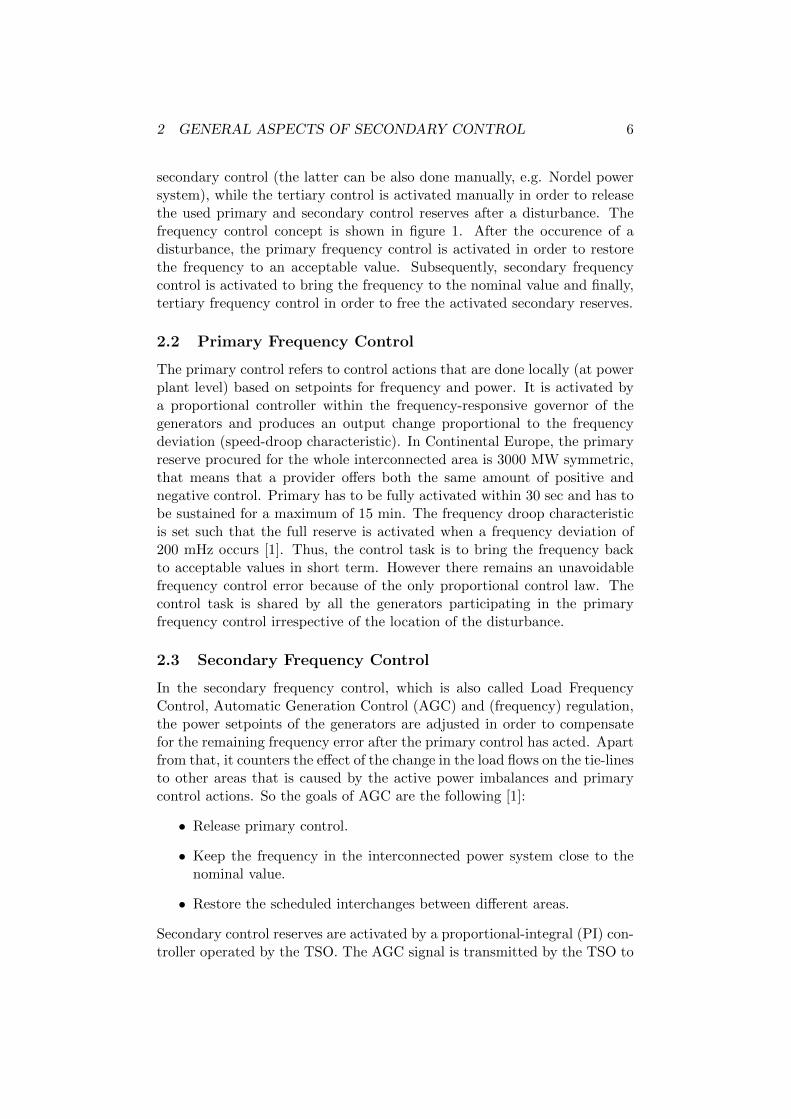
secondary control (the latter can be also done manually, e.g. Nordel powersystem), while the tertiary control is activated manually in order to releasethe used primary and secondary control reserves after a disturbance. Thefrequency control concept is shown in figure 1. After the occurence of adisturbance, the primary frequency control is activated in order to restorethe frequency to an acceptable value. Subsequently, secondary frequencycontrol is activated to bring the frequency to the nominal value and finally,tertiary frequency control in order to free the activated secondary reserves.
2.2 Primary Frequency Control
The primary control refers to control actions that are done locally (at powerplant level) based on setpoints for frequency and power. It is activated bya proportional controller within the frequency-responsive governor of thegenerators and produces an output change proportional to the frequencydeviation (speed-droop characteristic). In Continental Europe, the primaryreserve procured for the whole interconnected area is 3000 MW symmetric,that means that a provider offers both the same amount of positive andnegative control. Primary has to be fully activated within 30 sec and has tobe sustained for a maximum of 15 min. The frequency droop characteristicis set such that the full reserve is activated when a frequency deviation of200 mHz occurs [1]. Thus, the control task is to bring the frequency backto acceptable values in short term. However there remains an unavoidablefrequency control error because of the only proportional control law. Thecontrol task is shared by all the generators participating in the primaryfrequency control irrespective of the location of the disturbance.
2.3 Secondary Frequency Control
In the secondary frequency control, which is also called Load FrequencyControl, Automatic Generation Control (AGC) and (frequency) regulation,the power setpoints of the generators are adjusted in order to compensatefor the remaining frequency error after the primary control has acted. Apartfrom that, it counters the effect of the change in the load flows on the tie-linesto other areas that is caused by the active power imbalances and primarycontrol actions. So the goals of AGC are the following [1]:
• Release primary control.
• Keep the frequency in the interconnected power system close to thenominal value.
• Restore the scheduled interchanges between different areas.
Secondary control reserves are activated by a proportional-integral (PI) con-troller operated by the TSO. The AGC signal is transmitted by the TSO to

2 GENERAL ASPECTS OF SECONDARY CONTROL 7
the providing units in its control zone and it is dependent on the Area Con-trol Error (ACE), which should be controlled to zero. The power referencevalues of the generators participating in the AGC in an interconnected areawill be adjusted accordingly.
Figure 2: Control structure for AGC (∆ei = Error = ACEi = Area ControlError for area i) [1]
The ACE in Continental Europe is calculated according to eq. 1:
ACEi = PT i − PT0i +Bi · (f − f0) (1)
where:PT i is the measured value of the total power exchange with the other controlareas,PT0i is the scheduled power exchange with the other control areas,Bi is the frequency bias factor of the controlled area,f is the measured frequency andf0 is the set value of the frequency.A block diagram of such a controller is given in figure 2.
2.3.1 Current Status in Switzerland
Control Scheme The control scheme that is currently used by Swissgridis based on the classic PI controller. The ACE of the control area is derived

2 GENERAL ASPECTS OF SECONDARY CONTROL 8
by measurements of the tie-line interchanges and of the frequency deviationusing eq. 1. Then an analog PI controller is used to generate the AGCsignal that is dispatched to the participating units. The units receive anddiscretize the signal that adjusts their power setpoints, and consequentlythey change their power output in response to the signal.
Prequalification Procedure In order to be allowed to provide secondaryfrequency control, the generating units are subject to specific technical re-quirements that ensure the delivery of the control power demanded in real-time. The TSO of Switzerland, Swissgrid, requires that all generating unitsthat contribute to the market-based tenders of secondary control must bechecked to ensure they meet the necessary technical conditions [37]. Theappropriate test assesses the reaction of the generating unit to the test sig-nal that is provided by Swissgrid (figure 3) and is made available to theprovider by Swissgrid as a MW request.
The difference between the maximum and minimum power should be atleast 60% of the nominal output Pn. At each increase in power, the nominalminimum power provision is calculated using a PT1 element (time constant)according to eq.2. The time constant results from the requested gradientthat is 0.5 % of the nominal output per second
T1 =PmaxPn
· 1
0.005(2)
Furthermore, the actual power of the generating unit must be within thefollowing tolerance bands:
• Amplitude band: 5 % of the secondary control power to be provided.
• Negative dead time 10 s
• Positive dead time 20 s
All values in excess of the band are added together and applied across theentire signal. They must not be more than 1 % of the area covered by thesignal. The following formula illustrates this process:
[∑t
0 |Pdiff |] · ttPsec · t
· 100% ≤ 1% (3)
where:Psec is the distance between maximum and minimum secondary controlpower,Pdiff is the values in excess of the band,t is the test duration andtt is the sampling rate.

2 GENERAL ASPECTS OF SECONDARY CONTROL 9
Figure 3: Test signal for LFC for Switzerland [37]
Procurement, Deployment and Settlement Swissgrid procures sec-ondary frequency control reserves market-based, by organizing one-sidedweekly auctions [41]. The procurement is based on power reserve offers sup-plied by the participating providers into the secondary control market. Oneshould note that this market has specific features, namely the providersbid block offers, which only can be accepted or rejected but not partialyrequested, and also they can bid conditional offers, thus mutually exclu-sive bids. The market clearing is done against a predetermined demand,based on the two aforementioned rules, and aiming at the minimization ofprocurement costs.
The deployment of reserves is done pro-rata, i.e. in parallel for all theunits that have been accepted in the market. Each provider, based on theallocated capacity from the market, is responsible for providing a percentageof the dispatched AGC signal, so he receives at each point in time thededicated percentage of the signal. As regards the compensation for theservice, it is constituted by two components. One is the pay-as-biddedprice in the market for the reservation. The second is a remuneration ofthe activated control energy averaged every 15 minute intervals, where theenergy price is indexed by the respective price coming from the swiss energymarket [41].
2.4 Tertiary Frequency Control
Tertiary control reserve is manually activated and is usually used to relievethe secondary control reserves. It must be fully activated 15 minutes afterthe call from the dispatcher [41] .

3 ANALYSIS OF SECONDARY CONTOL HISTORICAL DATA 10
3 Analysis of Secondary Contol Historical Data
In this section historical data of power imbalances are analyzed with theaim to identify trends in the data, or certain patterns that can be taken intoaccount when planning and designing the automatically activated controlreserves products. For this analysis, historical data of ACE and activatedAGC with 10 seconds granularity are provided by Swissgrid for the monthsof July 2012 till January 2013.
3.1 Construction and Observation of Power Imbalances
As presented in chapter 2, the ACE is used to indicate the power balanceof the control area and is used as the input to the AGC system. This sys-tem generates and dispatches the AGC signal which automatically controlsthe resources participating in the secondary frequency control service. Thepower imbalances that have to be covered by the secondary frequency controlreserves can be calculated as in eq.4.
SEC(t) = −ACEopenloop(t) = −ACE(t) +AGC(t− 1) (4)
where:ACEopenloop is the ACE that would be observed if no secondary frequencycontrol is performed in the control area by the TSO,ACE is the closed loop error observed by the system andAGC(t − 1) is the activated secondary frequency control reserves in theprevious time step.This SEC represents the secondary frequency control needed to regulate theACE to zero. Figure 4 presents the control reserves required for 1st July2012:

3 ANALYSIS OF SECONDARY CONTOL HISTORICAL DATA 11
Figure 4: Secondary frequency control demand curve
As a first step to identify possible trends in the power imbalance signalthe average of the signal over one month is plotted. This is done for fourmonths in different periods of the year; namely July, August and November2012 and January 2013. The average imbalance is calculated as the verticalsummation of all the values of the same time step for every day of the month(eq.5).
SECavg(t) =1
N·N∑n=1
SECn(t) (5)
Figures 5 to 8 present the average secondary control demand for theaforementioned months.
Figure 5: Average secondary controlcurve for July 2012
Figure 6: Average secondary controlcurve for August 2012

3 ANALYSIS OF SECONDARY CONTOL HISTORICAL DATA 12
Figure 7: Average secondary controlcurve for November 2012
Figure 8: Average secondary controlcurve for January 2013
From the figures above a trend can be observed, especially in the timeslots of 00:00 - 03:00, 06:00 - 09:00 and 21:00 - 24:00, in all four months.This trend in the secondary control demand is probably a result of thecurrent european energy market setup with hourly traded products, an issueillustrated in the literature. In order to identify specific cyclic componentsthat constitute the observable trend in the signal, in the next section Fourieranalysis is applied on the average signal.
3.2 Discrete fourier Transform on the Power Imbalance Sig-nal
Since the time domain plotting of the secondary control does not revealany specific information on the dominant signal dynamics, the conversion ofpower signal sequence from time domain to frequency domain using DiscreteFourier Transform (DFT) is performed.
3.2.1 Mathematical Formulation of DFT
DFT converts a finite list of equally spaced samples of a function into a listof coefficients of a finite combination of complex sinusoids, ordered by theirfrequencies. The frequencies of the output sinusoids are integer multiples ofa fundamental frequency, whose corresponding period is the length of thesampling interval. The combination of sinusoids obtained through the DFTis periodic with the same period. The analysis function of DFT is [26]:
Y [k] =N−1∑t=0
y[t] · exp−j·(2·πN
)·t·k, k = 0, 1, . . . , N − 1 (6)
where:y[t] is the input sequence and

3 ANALYSIS OF SECONDARY CONTOL HISTORICAL DATA 13
Y [f ] is the output sequence of complex coefficients.The inverse DFT equation is the following:
y[t] =1
N·N−1∑k=0
Y [k] · exp−j·(2·πN
)·t·k, t = 0, 1, . . . , N − 1 (7)
With the use of DFT, each frequency component can be expressed inpolar form, characterized by the magnitude and phase. The original signalcan be expressed as a sum of cosines of all the frequency components:
y[t] =A0
2+
N2∑
n=1
An · cos(2 · π · fn · t+ φn) (8)
where:A0 is the dc offset (zero frequency component),An =
√Re(Y [k])2 + Im(Y [k])2 is the amplitude of the frequency compo-
nent,φn = arctan( Im(Y [k])
Re(Y [k]) ) is the phase of the component andfn is the frequency component.
3.2.2 Application on Historical Data
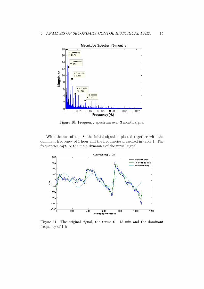
Regarding the historical data available, the Fast Fourier Transform (FFT)is applied on the averaged data for a whole day, namely 24 hours, andthen on the average data of the 3-hour time slots 00-03, 06-09 and 21-24.Figure 9 presents the results of the time slot 00-24 and 21-24 of the averagesignal of July, and figure 10 the FFT results of the actual historical signalover 3 months, (July-September 2012). Table 1 summarizes the dominantfrequency component observed. From the figures it can be seen that thepredominant frequency corresponds to the 1-hour component, as a result ofthe hourly energy market, and also, cyclic components of 30min, 15 min andless are observed. These can be attributed to ramping and fluctuations ofload and generation.

3 ANALYSIS OF SECONDARY CONTOL HISTORICAL DATA 14
(a) Frequency spectrum of the 24h averaged signal
(b) Frequency spectrum of the 21-24 time slot of the averaged signal
Figure 9: Frequency spectrum
Table 1: Frequency components
Frequency [Hz] Period
0.000278 1 h
0.000556 30 min
0.001111 15 min
0.001617 10 min
0.003333 5 min
0.01667 1 min
3 ANALYSIS OF SECONDARY CONTOL HISTORICAL DATA 15
Figure 10: Frequency spectrum over 3 month signal
With the use of eq. 8, the initial signal is plotted together with thedominant frequency of 1 hour and the frequencies presented in table 1. Thefrequencies capture the main dynamics of the initial signal.
Figure 11: The original signal, the terms till 15 min and the dominantfrequency of 1-h

4 ASYMMETRIC SECONDARY CONTROL 16
4 Asymmetric Secondary Control
A first option to increase the flexibility of providers, which are participatingor can potentialy participate in the secondary frequency control, is the pro-curement of asymmetric secondary control instead of the current symmetricprocurement. The implications of this change, both for the providers as wellas for the TSO are investigated in this section.
4.1 Implications for the Providers
In the current procurement scheme, the restriction for provision of symmet-ric secondary frequency control dictates to all potential providers that theymust have always the available contracted power capacity in both directions,i.e. to be able to increase generation output or to reduce consumption forpositive frequency control and at the same time to be able to reduce pro-duction or increase consumption for negative frequency control, if requested.In addition they should have enough energy stored in case of hydro storagepower plants and storage devices or available energy to modulate in case ofloads, which is delivered when positive (up) reserves are activated.
Each resource is awarded secondary reserves for the tendered week, there-fore it is obliged to keep the above mentioned required power and energycapacity margins for both directions for the whole week. This imposes re-strictions on the available amount that a provider can bid in the energymarket. Therefore these restrictions incur some costs to the participants,which are lost opportunity costs. Various technologies have different oppor-tunity costs [16], e.g. for hydro power plants is associated with the waterinflows and the respective water value, for wind power plants is related tothe lost revenue of energy that could have been earned from the energy pro-duction and sale [4]. If one analyzes the total cost of providing secondaryreserves, four elements can be identified:
• Upward reservation cost
• Downward reservation cost
• Upward utilization cost
• Downward utilization cost
The utilization is compensated by the energy compensation settlement,which account for wear and tear costs as well as fuel costs etc. The reserva-tion costs are related to the opportunity cost and the lost fexibility of a unitto produce at the whole operation range. Figure 12 shows the allocation ofa unit capacity and its opportunity cost.

4 ASYMMETRIC SECONDARY CONTROL 17
Figure 12: Capacity allocation of generating unit and associated costs
The opportunity costs can be unequal and therefore it can result in asym-metrical offers. Hence, by giving the possibility to providers to get awardedonly positive or only negative secondary, they can optimize their biddingbased on their true costs for providing the service, without having incurredcost by the compulsory provision in both directions. In the following, asimplifying example is presented:
Assuming that a unit has Pmax = 100MW capacity and Pmin = 40MWtechnical minimum. If the provider wants to provide 20 MW negative sec-ondary control, with the current setup would have to provide ±40MW .Therefore, the provider would be obliged to operate the unit at a level thatcan increase or decrease its output by 40 MW. Hence the operation point is,
60MW = Pmin − 40MW ≤ Pop ≤ Pmax − 40MW = 60MW (9)
So, the provider would have to bid only 60 MW in the energy market, andreserve the 40 MW for the frequency control. Thus the unit forgo potentialrevenue of 40MWh · Priceenergy. On the other hand, if the provider hadthe possibility to bid asymmmetric, in this example he could have biddedonly 40 MW negative. Hence, he would be able to bid up to 100MW in theenergy market, since up reservation is no longer compulsory.
4.2 Implications for the TSO
The TSO should expect changes in the price offers, as well as in the bid-ded volume per direction. Two contradicting phenomena can potentialy beobserved. On the one hand, more participants would join the market for

4 ASYMMETRIC SECONDARY CONTROL 18
each individual service, something that lead to higher liquidity and morefair prices. On the other hand, some of the participants that now provideoffers for the symmetric product, they can choose to participate only to oneof the two directions.
4.2.1 Impact on Reserve Dimensioning
As regards the determination of reserves, having asymmetric reserves canlead to different amount of reserves procured per direction. The methodused by Swissgrid for the dimensioning of secondary control reserves is aprobabilistic approach based on the deficit probability [19], which requiresthat ACE is regulated to zero 99.9% of cases. The approach consists of thefollowing steps:
1. Historical data of the ACE and activated control reserves are summedusing eq.4, to construct the power imbalances that have to be coveredby secondary (SEC).
2. A probability density function (PDF) of SEC is constructed.
3. Cumulative distribution function (CDF) is derived from the PDF andthe amount of reserves that respect the deficit level is determined.
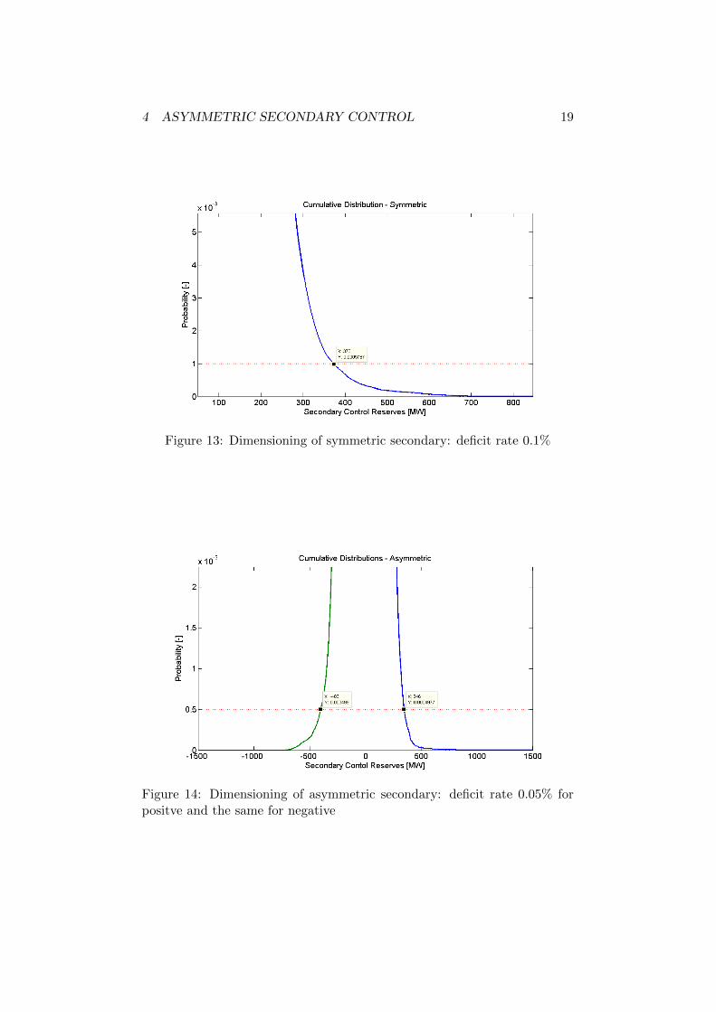
In the last step, which is the construction of CDF, no distinction is made forpositive and negative reserves, whereas absolute values of SEC are consid-ered, in the case of symmetric secondary. On the other hand, for asymmetricprocurement, a distinction have to be made between positive and negativereserves. As an example, figures 13 and 14 presents the CDFs for symmetricand respectively asymmetric secondary frequency control, derived from 3-month data of July to September 2012. As can be seen from the figures, thesymmetric secondary control results in ±373MW , while the asymmetric oneallocate - 403 MW negative secondary and 346 MW positive secondary. Thethreshold deficit rate is 0.1% for secondary positive and negative together(symmetric case), whereas it is 0.05% for each direction in the asymmetriccase.
4.2.2 Adjustment of Participation factors
The activation of secondary reserves is done pro-rata (parallel), i.e. each unitis activated proportionally to the amount of reserves it is awarded dividedby the total secondary control reserves. Hence the participation factor of itsunit, i, is defined as:
pfi =PiD
(10)
4 ASYMMETRIC SECONDARY CONTROL 19
Figure 13: Dimensioning of symmetric secondary: deficit rate 0.1%
Figure 14: Dimensioning of asymmetric secondary: deficit rate 0.05% forpositve and the same for negative

4 ASYMMETRIC SECONDARY CONTROL 20
where:Pi is the awarded secondary control capacity of the unit andD is the total amount of secondary cotnrol reserves.
In case of asymmetric secondary, a unit can have awarded differentamount of reserves in each direction (or even towards only one direction),thus the participation factors are changed to:
pfi =
Pup,iDup
, AGC(t) > 0Pdown,iDdown
, AGC(t) < 0(11)
where:pfi is the participation factor for unit i,Pup,i is the awarded positive secondary control capacity of the unit,Pdown,i is the awarded negative secondary control capacity of the unit,Dup is the total amount of positive secondary control reserves andDdown is the total amount of nagative secondary control reserves.

5 ADJUSTMENTS OF CONTROL CONCEPT 21
5 Adjustments of Control Concept
In this section two different concepts that adjust the current secondary fre-quency control scheme are presented. The target is to create a control setupthat generates control signals which are suitable to be followed by varioustechnologies that are subjected to different constraints. We focus on divid-ing the current AGC signal into a slow-changing, ramp-limited signal andinto a volatile one.
5.1 Filtering
The power imbalances that have to be covered by the secondary frequencycontrol service follow specific patterns due to the current Swiss and Europeanenergy market setup. Specifically five dominant cyclic components wereidentified (see table 1). The approach examined in this section is based onthe observed frequency dynamics and refers to the division of AGC signalas derived from the output of the PI controller. Resources that are capableof fast ramping, or those that can follow the changes in dispatched signaldirections with lower wear and tear, can assume the fastest-cyclic portion ofthe AGC signal, whereas other type of technologies can follow the smootherlower-cyclic portion. The general filtering scheme is presented in figure 15.Since the goal is to partition the AGC signal in real-time, only causal filtersare investigated.
Figure 15: Filtering of the output of PI controler and creating two controlsignals
In this analysis five types of filters are examined. These are:
• Finite Impulse Response lowpass filter (FIR)
• Infinite Impulse Response (IIR) Butterworth lowpass filter

5 ADJUSTMENTS OF CONTROL CONCEPT 22
• Infinite Impulse Response (IIR) Chebyshev type I lowpass filter
• Exponential Weighted Moving Average (EWMA) filter
• Infinite Impulse Response (IIR) Chebyshev type I highpass filter
Each filter type has advantages and disadvantages that are mentioned ineach specific section in the sequel.
5.1.1 Lowpass Filter Setup
One proposed setup is to direct the AGC signal through a low-pass filter,from which the low frequency part of the signal is extracted and then itsresidual is obtained. This residual contains the high frequency part, takenby subtracting the low-frequency component from the originial signal. Thescheme is presented in figure 16
Figure 16: Filtering of the output of PI controler with a lowpass filter
Finite Impulse Response Filters The first filter type examined is thelinear-phase FIR. These filters approximate unity transmission in the pass-band and zero transmission in the stopband. There are several methods fordesigning such filters (ch.7 in [26]). A common used method is the windowmethod. According to this method, the ideal frequency response is trun-cated using a window function. Matlab’s function ”fir1” is used to produceFIR filters of specified order using a Hamming window [26]. The transferfunction of this filter type contains only zeros and no poles as shown in eq.12.
H(z) =N∑n=0
bn · z−n (12)
A main advantage of the FIR filters is the potential for steep frequencycutoff and low stopband transition bandwidth. This ensures that the high-frequency components are wiped out. A further advantage is the linear phase

5 ADJUSTMENTS OF CONTROL CONCEPT 23
characteristic, which means that the signal is not distorted by the filter andresults in a smooth step response without overshoot. The disadvantage ofthe FIR filters is the relatively large delay occured due to the usually higherorder of those filter types. Due to the linear phase characteristic, thesefilters impose a constant delay over the whole frequency spectrum, whichis determined for a filter of order N by the relation: N+1
2 samples. Thisdelay can cause problems when such type of filters are used in real timeoperation. When the filter is of high order, the delay is large and the filteris not suitable for real time operation, in this case for signal seperation in asecondary frequency control scheme.
The first FIR filter under investigation is of high order (201st) so asto exhibit good approximation of the ideal cutoff characteristic for a cutofffrequency corresponding to 15 min. As the available data are sampled with10-seconds sampling frequency, the filter has approximately a 17 minutesdelay. In figure 17 the taps’ weights of the filter as well as the frequencyresponse of this filter are presented, while figure 18 presents the output ofthe filter. As can be observed from the graphs, the filter smooths the initialsignal, and attenuates the higher frequencies, but it cannot be used in realtime secondary frequency control due to the large delay.

5 ADJUSTMENTS OF CONTROL CONCEPT 24
Figure 17: Frequency response and taps’ weights of 201 order FIR filter
5 ADJUSTMENTS OF CONTROL CONCEPT 25
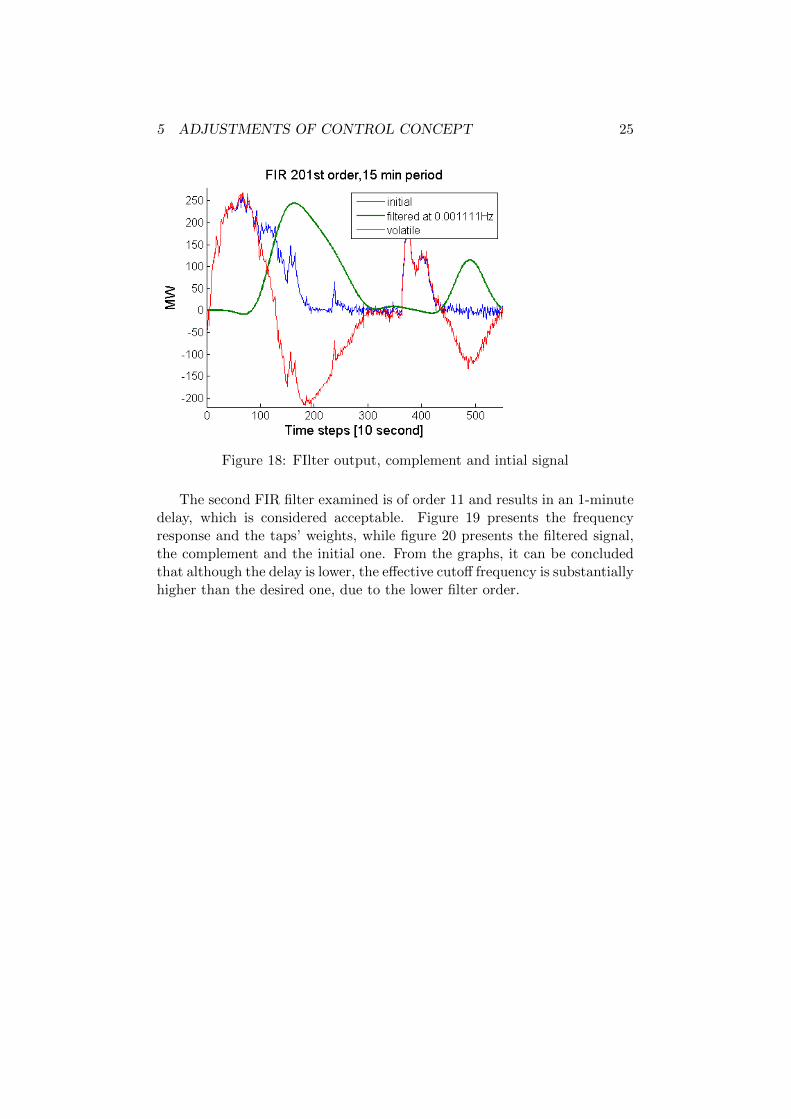
Figure 18: FIlter output, complement and intial signal
The second FIR filter examined is of order 11 and results in an 1-minutedelay, which is considered acceptable. Figure 19 presents the frequencyresponse and the taps’ weights, while figure 20 presents the filtered signal,the complement and the initial one. From the graphs, it can be concludedthat although the delay is lower, the effective cutoff frequency is substantiallyhigher than the desired one, due to the lower filter order.

5 ADJUSTMENTS OF CONTROL CONCEPT 26
Figure 19: Frequency response and taps’ weights of an 11-order FIR filter

5 ADJUSTMENTS OF CONTROL CONCEPT 27
Figure 20: Filter output, complement and initial signal
Infinite Impulse Response Filters As a next step, two classes of Infi-nite Impulse Response (IIR) filters are investigated. The primary advantageof IIR filters over FIR is that they typically need much lower order for thesame specifications. On the contrary, they have nonlinear phase, whichmeans that the delay is a function of frequency (not a constant value as inthe case of FIR filters). The IIR filter transfer funnction is presented in eq.13.
H(z) =
∑Pn=0 bn · z−n
1 +∑Q
m=1 am · z−m(13)
A 3rd-order Butterworth and a 3rd-order Chebyschev type I low-pass filtersare designed in matlab using the respective built-in functions. The order ofthe filter is selected in such a way, to achieve a good trade-off between afaster roll-off and an increased delay due to the additional poles [26]. TheButterworth filter has a magnitude maximally flat in the passband and asmooth transition band. The frequency response and the output of a filterwith a 15-minute cutoff frequency are presented in figure 21.

5 ADJUSTMENTS OF CONTROL CONCEPT 28
Figure 21: Frequency response and fIlter output 3rd order low-pass Butter-worth, complement and intial signal
The Chebyshev type I filters are characterized by equiripple magnitudein the passband and monotonic magnitude in the stopband. The Chebyshevfilter has a good attenuation of high frequencies and a steeper roll-off thanthe Butterworth filter of the same order. The frequency response and theoutput of a filter with a 15-minute cutoff frequency are presented in figure22. Both filter types exhibit a lower delay than the FIR filters, a goodperformance in the frequency domain and can potentially be used in realtime operation.

5 ADJUSTMENTS OF CONTROL CONCEPT 29
Figure 22: Frequency response and filter output 3rd order low-pass Cheby-shev type I, complement and intial signal
Exponential Weigted Moving Average Finally the last category oflow-pass filters examined is the Exponential Weighted Moving Average filter(EWMA). This is equivalent to a 1st order IIR filter with the followingtransfer function:
yk = a · xk + (1− a) · yk−1 (14)
where a = ∆TTfilter+∆T is the smoothing factor and
Tfilter = 12πf is the equivalent analog filter time constant.
The frequency response and the resulting output of the filter are plotted infigure 23. As it can also be observed from the figure, the EWMA filters are
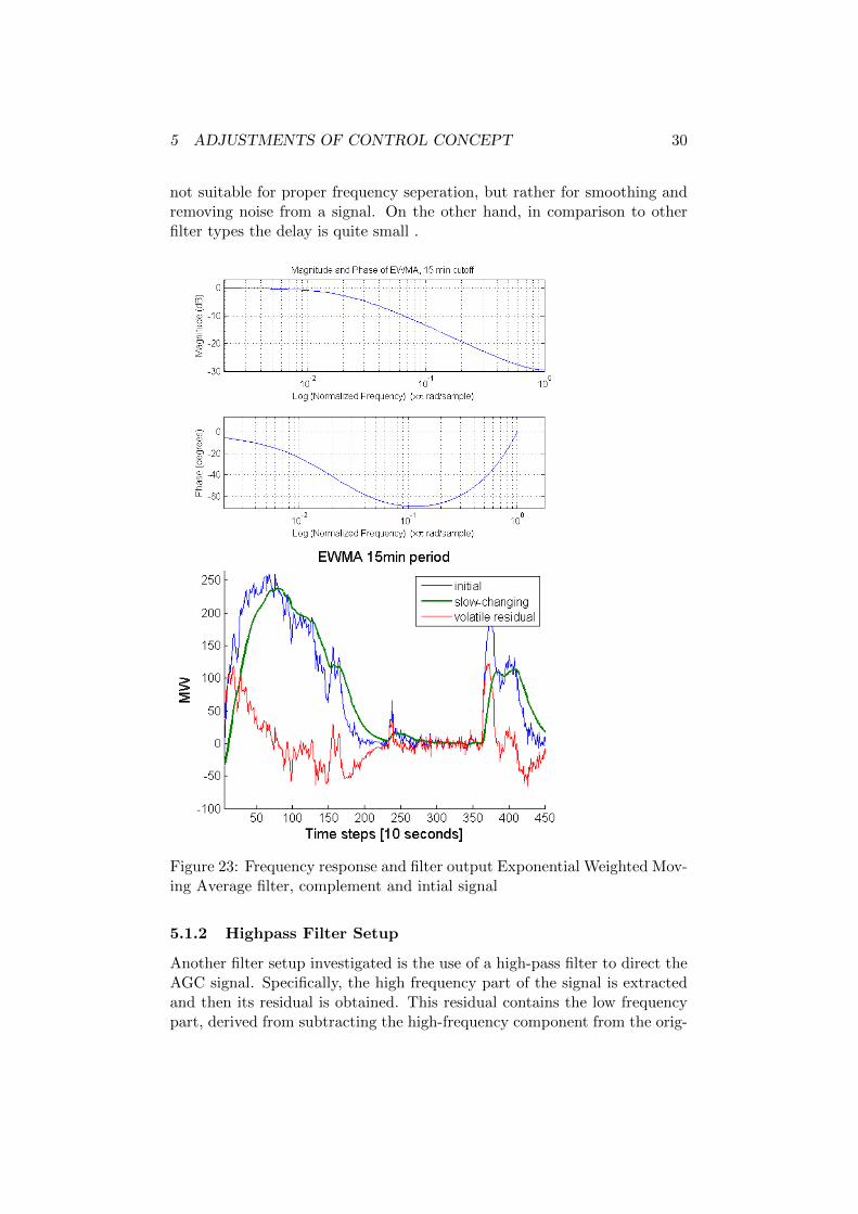
5 ADJUSTMENTS OF CONTROL CONCEPT 30
not suitable for proper frequency seperation, but rather for smoothing andremoving noise from a signal. On the other hand, in comparison to otherfilter types the delay is quite small .
Figure 23: Frequency response and filter output Exponential Weighted Mov-ing Average filter, complement and intial signal
5.1.2 Highpass Filter Setup
Another filter setup investigated is the use of a high-pass filter to direct theAGC signal. Specifically, the high frequency part of the signal is extractedand then its residual is obtained. This residual contains the low frequencypart, derived from subtracting the high-frequency component from the orig-

5 ADJUSTMENTS OF CONTROL CONCEPT 31
inal signal. This setup is presented in figure 24.
Figure 24: Filtering of the output of PI controler with a high-pass filter
In this case only a 3rd-order Chebyschev type I high pass filter is investi-gated, and the frequency response as well as the filter output are presentedin figure 25. As it can be observed from the figures, the high-pass filter hasa lower delay than the low-pass IIR filter and good frequency response. Onthe other hand, the slower-changing signal, that contains the low frequencydynamics, appears to be less smooth and also exhibits an overshooting atthe maximum value compared to the signals of the low-pass filters.

5 ADJUSTMENTS OF CONTROL CONCEPT 32
Figure 25: Frequency response and fIlter output 3rd order highpass Cheby-shev type I, complement and intial signal
5.1.3 Comparison of Filters
In order to compare the filters presented in the previous section in terms oframping-rate requirement of the slow-changing signal and energy require-ment of the volatile signal, ramp-rate duration curves and energy durationcurves are used, as presented in the literature [17]. The ramp-rate dura-tion curve is the visual representation of the fraction of time that a certaintotal ramp-rate is required from the generating unit. The energy durationcurve determines the net energy required at each time instant and showsthe percent of time that the net energy requirement is at or below a certainlevel [17]. The average absolute ramp-rate versus the maximum energy areplotted as proposed in reference [17].
Firstly, the average ramping rate for the period July 2012 till September

5 ADJUSTMENTS OF CONTROL CONCEPT 33
2012 for the slow-changing signal produced by the Butterworth, Chebyshev,EWMA and high-pass Chebyshev filters for cutoff frequencies of 15 min,10 min and 1 min is identified and then, the absosute energy of the volatilesignal for the above filters and cutoffs is calculated. The results are plotted infigure 26. It can be observed that the higher the delay of the filter, the morethe energy required from the volatile signal, because the time lag betweenthe low-frequency slow-changing signal and the initial one results in a largearea that must be covered from the resources following the volatile signal.Therefore, the energy requirement increases. The high-pass Chebyshev filtercompared to the low-pass one exhibits higher ramping requirement for theslow-changing signal. However, it requires substantially less energy for thevolatile one. Finally, the EWMA filter that has the lowest time delay (dueto lower order) appears to have a moderate ramp-rate requirement for theslow signal and a low energy requirement for the units following the volatilesignal.
Figure 26: Mean absolute ramping rate vs Maximum energy for four filtertypes. The cutoff frequencies are the same for every filter and their valuesare marked in the diagrams for 15 min, 10 min, 5 min, 1 min, from left toright respectively
In order to identify how the ramping requirement and the energy requiredchange when applying different cutoff frequencies, the ramp-rate durationcurves and the energy duration curves are plotted. The low-pass Chebyshevtype I filter is used to illustrate the change in the ramping rate and energyrequirement as the cutoff frequency is changing from lower frequencies tohigher ones. The frequencies examined here are those identified in section3.2 from the analysis in the frequency domain. Figure 27 presents the ramp-

5 ADJUSTMENTS OF CONTROL CONCEPT 34
rate duration curves of the slow-changing signal as a derived output of thelow-pass Chebyshev filter with cutoff frequencies at 1 h, 30 min, 15 min, 10min, 5 min and 1 min, while figure 28 presents the energy duration curve ofthe residual volatile signal for each cutoff frequency. From the figures, it isobvious that the low-pass filter smoothes the initial AGC signal, thereforethe ramping requirement of the filtered signal is substantially reduced incomparison to the initial one. From the plots it can also be seen that eventhough the ramp-rate duration curves and the energy duration curves areflat for the majority of the time, they exhibit long and steep tails. Thismeans that the high ramp-rate and energy requirement are rarely used.
Figure 27: Ramping-rate duration curves of slow changing signal for differentcutoff frequencies, lowpass Chebyshev filter

5 ADJUSTMENTS OF CONTROL CONCEPT 35
Figure 28: Energy duration curves of the volatile signal for different cutofffrequencies
Finally figure 29 presents the average ramp-rate versus the maximumenergy requirement. From the figure it can be derived that the lower thecutoff frequency:
I. the lower the ramp-rate requirement of the smooth signal
II. the higher the energy storage requirement of the volatile signal.
Figure 29: Mean absolute ramping rate vs Maximum energy for lowpassChebyshev filter

5 ADJUSTMENTS OF CONTROL CONCEPT 36
Besides the ramping and the energy requirement, the number of changesin signal direction is of interest. This is the case especially for some typesof loads, which have to respect a duty cycle e.g. 15 minutes time, betweenswitching on/off [12]. If the unit that follows the dispatched AGC signal is anaggregator of many heat pumps, for example, when the AGC signal changesfrom increasing to decreasing, many devices would have to switch off. Thiscan limit the available bidding volume of the provider, when the aggregatoris not consisted of a large pool or when the signal changes direction toooften within an hour in comparison to the individual duty-cycle time of thedevices (e.g. 15 min). Since the volatile signal takes the high frequencycomponents, one is expecting to detect many changes in direction, whereasfrom the slow-changing signal, which is smoother and is consisted of lowfrequency components, only few changes. In order to examine that, thenumber of changes in direction within 1 hour are counted. For each hourthese are defined as:
change(t) =
1, sgn(s(t)− s(t− 1)) 6= sgn(s(t− 1)− s(t− 2)),
0 sgn(s(t)− s(t− 1)) = sgn(s(t− 1)− s(t− 2)),(15)
where:change(t) is the variable to count for the current time step,t denotes the current time step,s(t) is the AGC or the slow-changing AGC signal sgn is the sign function
sgn(x) =
−1, x < 0,
0, x = 0,
1, x > 0.
The number of changes within 1 hour is defined as:
ND =
N=360∑t=1
change(t) (16)
In order to identify a bound on the expexted number of changes per hour,the probability of occurence is calculated and cumulative distribution curvesare ploted. Figure 32 presents the cumulative distributions for Chebyshevlowpass and highpass and EWMA filter, for different cutoff frequencies. Thered line indicates the 95% probability.

5 ADJUSTMENTS OF CONTROL CONCEPT 37
Figure 32: Cumulative distribution of number of changes in direction within1 hour for lowpass, highpass and EWMA filter
5 ADJUSTMENTS OF CONTROL CONCEPT 38
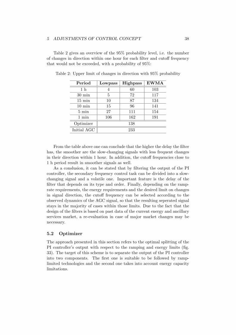
Table 2 gives an overview of the 95% probability level, i.e. the numberof changes in direction within one hour for each filter and cutoff frequencythat would not be exceeded, with a probability of 95%:
Table 2: Upper limit of changes in direction with 95% probability
Period Lowpass Highpass EWMA
1 h 4 60 103
30 min 5 72 117
15 min 10 87 134
10 min 15 96 141
5 min 27 111 154
1 min 106 162 191
Optimizer 138
Initial AGC 233
From the table above one can conclude that the higher the delay the filterhas, the smoother are the slow-changing signals with less frequent changesin their direction within 1 hour. In addition, the cutoff frequencies close to1 h period result in smoother signals as well.
As a conslusion, it can be stated that by filtering the output of the PIcontroller, the secondary frequency control task can be divided into a slow-changing signal and a volatile one. Important feature is the delay of thefilter that depends on its type and order. Finally, depending on the ramp-rate requirements, the energy requirements and the desired limit on changesin signal direction, the cutoff frequency can be selected according to theobserved dynamics of the AGC signal, so that the resulting seperated signalstays in the majority of cases within those limits. Due to the fact that thedesign of the filters is based on past data of the current energy and ancillaryservices market, a re-evaluation in case of major market changes may benecessary.
5.2 Optimizer
The approach presented in this section refers to the optimal splitting of thePI controller’s output with respect to the ramping and energy limits (fig.33). The target of this scheme is to separate the output of the PI controllerinto two components. The first one is suitable to be followed by ramp-limited technologies and the second one takes into account energy capacitylimitations.

5 ADJUSTMENTS OF CONTROL CONCEPT 39
Figure 33: Optimal splitting of the PI output with respect to ramping andenergy limits
The decision variables, the constraints and the objective function of theoptimization block are:
Decision Variables The decision variables are the power values of theslow-changing and of the volatile signal:(
xsxf
)where:xs [MW] is the power output of the ramp-limited component andxf [MW] is the power otuput of the volatile signal.
Constraints The slow-changing ramping signal is constrained by the max-imum and minimum reserves procured, i.e. the saturation constraints:
Ps,min ≤ xs ≤ Ps,max (17)
where:Ps,min [MW] is the minimum capacity of the slow-changing signal andPs,max [MW] is the maximum capacity of the slow-changing signal.
The ramping rate of the slow-changing signal is also contrained by max-imum and minimum limits:
ramps,min ≤ ramps ≤ ramps,max (18)
where:ramps,min [MW
s ] is the minimum ramping rate limit and

5 ADJUSTMENTS OF CONTROL CONCEPT 40
ramps,max [MWs ] is the maximum ramping rate limit.
Since the decision variables are power signals, the ramping limits shouldbe expressed in MW. The ramping rate can be approximated by the differ-ence between the current power output xs and the previous power outputvalue xs,prev, divided by the time step ∆t, i.e. 10 seconds in this case:
ramps =xs − xs,prev
∆t(19)
The minimum,us,min, and maximum, us,max, allowed deviations betweentwo consecutives time steps are calculated by the following relations:
us,min = ramps,min ·∆tus,max = ramps,max ·∆t
(20)
Therefore, eq.18 can take the following form:
us,min + xs,prev ≤ xs ≤ us,max + xs,prev (21)
The volatile signal is constrained by its upper and lower capacity limits thatcorrespond to the available procured amount in MW (saturation constraint):
Pf,min ≤ xf ≤ Pf,max (22)
where:Pf,min [MW] is the minimum capacity of the volatile signal andPf,max [MW] is the maximum capacity of the volatile signal.
Regarding the volatile signal, an additional constraint which takes intoaccount the total energy stored to or requested by the resources followingthat signal has to be considered. This can be meaningful for aggregateddemand response and storage technologies or hydro storage power plantsrelated to the consumption of water stored in their reservoir. Therefore theenergy value during the next time step of operation can be limited by:
Ef,min ≤ Ef,next ≤ Ef,max (23)
where:Ef,min [MWh] is the minimum energy requested by (the maximum storedinto) the devices following the volatile signal andEf,max [MWh] is the maximum energy requested by the devices followingthe volatile signal.
From the grid’s perspective, the energy requested from the devices isincreased when the power signal sent is positive, while it is decreased when

5 ADJUSTMENTS OF CONTROL CONCEPT 41
the power signal is negative. The relation between energy and power is givenby eq. 24:
Ef,next = Ef + xf ·∆t (24)
where:Ef [MWh] is the current total energy level added to or subtracted from theenergy basepoint of the unit following the volatile component of the AGCsignal.Therefore, by substituting eq. 24 into eq. 23 the following relation is derived
Ef,min ≤ Ef + xf ·∆t ≤ Ef,max (25)
Ef,min − Ef∆t
≤ xf ≤Ef,max − Ef
∆t(26)
where:Ef,min (e.g. -1000 MWh) is the minimum limit in energy for the volatilesignal andEf,max (e.g. 1000 MWh) is the maximum limit in energy for the volatilesignal.
Finally, the activated control reserves from both signals must equal thetotal AGC signal generated by the PI, which is the input to the optimizerblock. The constraint is presented in eq. 27
xs + xf = xSEC (27)
where xSEC is the total secondary frequency control needed.Summing up, the constraints imposed are:
xs,min ≤ xs ≤ xs,max
xs,min = max(Ps,min, us,min + xs,prev)
xs,max = min(Ps,max, us,max + xs,prev)
xf,min ≤ xf ≤ xf,max
xf,min = max(Pf,min,Ef,min − Ef
∆t)
xf,max = min(Pf,max,Ef,max − Ef
∆t)
xs + xf = xSEC

5 ADJUSTMENTS OF CONTROL CONCEPT 42
Objective function The aim is to penalize the deviation of the slow-changing signal’s ramp-rate from the zero value, as well as deviation ofthe energy injected or withdrawn by the volatile signal from the zero level.Therefore, the objective function consists of two quadratic cost terms (eq.28).
J = Costs + Costf = as(xs − xs,prev
∆t− 0)2 + cf (Ef,next − 0)2 (28)
where:as is a weighting factor for first term andcf is a weighting factor.The first cost term is th quadratic function for the slow-changing signal eq.29
Costs = as(xs − xs,prev
∆t− 0)2 = cs(x
2s + x2
s,prev − 2 · xs · xs,prev) (29)
where:cs = as
∆t is a weighting factor.
The second cost term is the quadratic cost function that penalizes thedeviation of the next energy level of the volatile signal from zero (eq. 30):
Costf = cf (Ef,next − 0)2 = cf (Ef + xf ·∆t)2) =
= cf (E2f + (xf ·∆t)2 + 2 · Ef · xf ·∆t) (30)
To sum up, the objective function is given by the following equation:
minXJ = cs(x2s − 2 · xs · xs,prev) + cf ((xf ·∆t)2 + 2 · Ef · xf ·∆t) (31)
Global minimization problem The objective function can be formu-lated as a global minimization problem:
Cost =1
2X ·H ·XT + fT ·X (32)
where:
X =
(xsxf
), H =
(2cs 00 2cf ·∆t2
), f =
(2csxs,prev
2cf · Ef ·∆t
)In order to identify the impact of the weighting factors in the respective
cost functions, the two cost functions are plotted for several values of these.Figure 34a presents the cost function of the ramping and figure 34b presentsthe cost function of the energy deviation from zero for different weightingfactors. As it can be seen from the graphs, if the two weights differ from each

5 ADJUSTMENTS OF CONTROL CONCEPT 43
(a) Cost function of ramping rate deviation
(b) Cost function of energy deviation
Figure 34: Cost functions for ramping quadratic term and energy quadraticterm

5 ADJUSTMENTS OF CONTROL CONCEPT 44
other by an order of thousands, e.g cs = 100, cf = 0.1 or cs = 1, cf = 0.001,then the two costs are of the same order and comparable.
As a further assesment of the impact of the weighting factors, the setupis used to split the real AGC dispatched signal of the 1st of July 2012in Switzerland. Figures 35 and 36 present the results for cf = 0.1 andcs = 10, 50, 100, 200, 300, 1000. When the volatile signal’s weighting factoris kept constant, it is observed that as the weighting factor of the slow-changing signal’s increases, the slow-changing signal is getting smoother.
As regards the the trade-off between the ramping rate of the slow-changing signal and the energy of the volatile signal, the duration curvesare used, together with cumulative distributions. The resulting ramping-rate and energy duration curves for the above combinations of weightingfactors ( cf = 0.1 and cs is changing) are presented in figures 37 and 38.Considering now the number of changes in slow signal direction within onehour, the figure 39 shows the cumulative probability curve resulting fromseperating 3-month AGC data (July-September 2012), with cf = 0.001 andcs = 1.
Figure 37: Ramping-rate duration curve of slow changing signal for differentweighting

5 ADJUSTMENTS OF CONTROL CONCEPT 45
Figure 35: AGC seperation with cs = 10, 50, 100

5 ADJUSTMENTS OF CONTROL CONCEPT 46
Figure 36: AGC seperation with cs = 200, 300, 1000

5 ADJUSTMENTS OF CONTROL CONCEPT 47
Figure 38: Energy duration curves of the volatile signal for different weight-ing
Figure 39: CDF of number of changes in direction of slow-changing signal
One can conclude from the graphs that the different weights shift theenergy and the ramping requirement between the two signals. If the weightsare set to a difference in order of thousands, the achieved results are similiarto those obtained by the EWMA filter with 15 min cutoff frequency. Basedon figure 39 the observed changes in direction within one hour, for a resourcefollowing the slow signal will not exceed the 138 with probability 95%.

6 TIME DOMAIN SIMULATIONS 48
6 Time Domain Simulations for Evaluation of Con-trol Performance
In this section the impact of the proposed technical concepts on the quality ofcontrol is investigated. This is done by conducting time-domain simulationson a power system model built in Matlab/Simulink.
6.1 Power System Modeling
In order to examine the impact of the proposed concepts on the qualityof secondary frequency control, a proper model of a power system haveto be developed. To obtain a dynamic model of a generic control area theassumption is made that the individual electrical connections within an areaare so strong (in comparison to the tie-lies between the adjoining areas), thateach area can be represented by a single frequency, i.e. all generators in asingle area swing together [10]. This means that the frequency dynamics ofthe system can be expresed by the lumped swing equation [1] as presentedin eq. 33:
∆f =f0
2 ·H · SB· (∆Pm −∆Pe) (33)
where:∆f is the deviation of the frequency from its nominal value,f0 is the nominal value of frequency,∆Pm is the deviation of the total mechanical power from its set point,∆Pe is the deviation of the total electrical power from its set point,
H is the total inertia time constant and is defined as H =
∑j Hj ·SBj∑j SBj
and
SB is the total rating power and is defined as∑
j SBj .
Since ∆Pe = ∆PLoad + ∆P freqLoad + ∆Ptie, one achieves:
∆f =[∆Pm − (∆PLoad +D ·∆f + ∆Ptie)] · f0
2 ·H · SB(34)
where:∆P freqLoad = D ·∆f is the frequency-dependent loads and D is the load damp-ing coeeficient,∆PLoad is the load deviation, i.e. the power imbalance in the system, and∆Ptie is the total tie-line interchanges with the adjoining areas.
The tie-line power for small deviations between area i and j is given byeq. 35 [1]:
∆Ptie =
N∑j=1j∈Ωi
Ui · UjXij
· cos(φ0,i − φ0,j) · (∆φi −∆φj) (35)

6 TIME DOMAIN SIMULATIONS 49
where:Xij is the equivalent reactance of the tie line andΩi denotes a set containing all areas j connected to area iSince ∆φ = 2 · π ·∆f , it can be derived:
∆ ˙Ptie = 2 · π ·N∑j=1j∈Ωi
Ui · UjXij
· cos(φ0,i − φ0,j) · (∆fi −∆fj) (36)
where:∆fi and ∆fj are the frequency deviations of areas i and j.
As regards the power plant dynamics, a thermal power plant can bedescribed by two first order tranfer functions, which represents the governorand the turbine dynamics, as given in eq. 37 and in eq. 38:
∆ ˙PV t =∆PAGC − 1
Sf·∆f −∆PV t
TC(37)
where:∆PV t is the output signal of the thermal turbine controller,∆PAGC is the setpoint sent by the secondary frequency controller,Sf is the speed droop characteristic of the generator andTC is the thermal turbine’s governor time constant.
∆ ˙PTt =∆PV t −∆PTt
TT(38)
where:∆PTt is the thermal turbine output andTT is the thermal turbine time constant.
A hydro power plant is described by hydro governor dynamics and tur-bine dynamics. Applying linearization by small signal analysis, the governordynamics are described by eq.39 and 40, while eq.41 presents the turbinedynamics:
G =∆PAGC − 1
RP·∆f −G
TG(39)
where:G is the hydro-governor’s first stage output,RP is the static (permanent) speed droop characteristic of the hydro gener-ator andTG is the governor time constant.
6 TIME DOMAIN SIMULATIONS 50
∆ ˙PV h =G+ G · TR −∆PV h
RTRP· TR
(40)
where:∆PV h is the second stage’s output of the hydro governor,TR is the reset timer,RT is the transient speed droop characteristic of the hydro andTc is the thermal turbine’s governor time constant.
∆ ˙PTh =∆PV h −∆PTh − TW ·∆ ˙PV h
0.5 · TW(41)
where:∆PTh is the hydro turbine output andTW is the water starting time.
Finally, for the modeling of the new technologies that can participate inthe secondary frequency control like aggregated controllable loads or energystorage devices several models can be used depending on the properties,the aggregation level, the type of devices in a load-pool etc. e.g.[43] and[45]. Here these technologies are modeled as ideal resources, which they canprovide accurately the capacity they have been awarded [21] and also theycan respond to the AGC signal instantaneously as [12].
In order to perform the simulations, a five-area interconnected powersystem is built in Matlab/Simulink as depicted in figure 40. Further, eacharea is represented by an aggregated model, that is consisted of the dynamicsof a single generator with turbine and governor dynamics.

6 TIME DOMAIN SIMULATIONS 51
Figure 40: Five area interconnected power system
Each of four areas are modeled as a representative thermal power plant,and hence the transfer functions for the thermal turbine and governor areused (figure 41), so ∆Pm = ∆PV t . Since the majority of power plants inSwitzerland that participate in the secondary frequency control are hydroplants, the fourth control area is represented by a hydro power plant, thusthe transfer functions of hydro gevernor and turbine are used in this case,figure 42. In this area, controllable devices can also deliver part of thedispatched agc signal based on the pf1 and pf2, which are the participationfactors. Therefore ∆Pm = pf1 ·∆PV t + pf2 ·∆PAGC .

6 TIME DOMAIN SIMULATIONS 52
Figure 41: An area modeled with thermal power plant
Figure 42: An area modeled with hydro power plant
The state space formulation can be used to represent mathematicallythe power system (eq. 42):
xk+1 = A · xk +B · uk,yk = C · xk
(42)

6 TIME DOMAIN SIMULATIONS 53
where:xk is the state vector at time step k,uk is the input vector at time step k,yk is the output vector at time step k,A is the state matrix,B is the input matrix andC is the output matrix.In case of areas modeled as thermal power plant the state, input and outputvector are:
x =
∆f
∆Ptie∆PTt∆PV t
, u = ∆PAGC , y = ACE (43)
Whereas for the area which is modeled as a hydro power plant are:
x =
∆f
∆Ptie∆PTh∆PV hG
, u = ∆PAGC , y = ACE (44)
The adjustments in the controller, are those depicted in figures 16, 24and33. The transfer function described in eq. 13 for the modelling of thefilters, with their respective coefficients, is inserted into the AGC schemefor the first two cases. For the optimizer, the algorithm is implemented inTomlab and Matlab, and is inserted as an S-function into the AGC schemein Simulink model.
6.2 Time-Domain Simulations
In order to investigate whether there is any impact on the quality of controldue to the proposed changes to the controller (as described in section 5) thefollowing scenarios are simulated:
1. Comparison of base-case, i.e. current AGC scheme with participationof only hydro power plants, to the control scheme that adjust the PIoutput by filtering or by optimizer, where the slow signal is followedby hydro and the volatile signal only by controllable devices: pfs1 = 1,pfs2 = 0, pff1 = 0 and pff2 = 1
2. Comparison of current AGC scheme with participation of 70% hydroand 30% controllable devices, to the case of the adjusted PI outputwith the same participation (70% - 30%) for both slow and volatilesignal: pfs1 = 0.7, pfs2 = 0.3, pff1 = 0.7 and pff2 = 0.3

6 TIME DOMAIN SIMULATIONS 54
The following information apply to both scenarios:
• For the implementation of the first concept the cutoff frequency thatcorresponds to 15 minute period is used.
• The filters implemented are: lowpass Chebyshev, highpass Chebyshevand Exponential Weighted Moving Average
The parameters of the optimizer used in the both scenarios are presented intable 3;
Table 3: Parameters of simulation
Parameters value Parameters value
N 1 us,max 50 MW
∆t 10 s us,min -50 MW
cf 0.001 uf,max ∞rs 1 uf,min −∞
xs,max ∞ MW Ef,max ∞xs,min -∞ MW Ef (0) 0 MWh
xf,max ∞ MW xs(0) 0 MW
xf,min -∞ MW xf (0) 0 MW
The modeling of areas 1, 2, 3 and 5 remains the same in all scenariosexamined. The model of area 4 as presented in figure 42 represents the cur-rent secondary frequency control setup with one non-splitted signal. Figure43 presents the model of control area adjusted for the splitted secondary fre-quency control, in which there are seperate participation factors for the unitsfollowing the slow-changing signal pfsi and those that follow the volatile onepffj .

6 TIME DOMAIN SIMULATIONS 55
Figure 43: An area modeled with hydro power plants and controllable de-vices
In every scenario two cases are examined. First a step load increase of300 MW is inserted as power imbalance in the system modeled as hydro(area 4) and the resulting Df in the system and dispatched AGC signal(s)are compared. In the second case real power imbalances data for 3 months,that have to be covered by secondary frequency control, are imposed tothe system for every scenario. The power imbalance signal is a continuousone, which is re-composed from the SEC data by applying eq. 8. In orderto evaluate the impact on the quality of control the probability densityfunctions of the ACE are plotted.
In order to identify the difference in response due to the different technol-ogy mix in the two scenarios (100% hydro vs 70% hydro and 30% other typeof units) the frequency deviation with the current AGC scheme is plottedin figure 44

6 TIME DOMAIN SIMULATIONS 56
Figure 44: Df resulting fro step increase in load 300 MW
From figure 44 it can be seen that the 70%:30% generation mix resultsin less frequency deviation, and the overall control shows improved perfor-mance. So, one can expect, that in the first scenario where the current setuputilizes only hydro, whereas the new setup utilizes only ideal resources tofolllow the fast signal, one will observe better results from the new setup.On the other hand, in the second scenario where the same generation mixis used in both current and proposed setups, any change in the performancewill be due to the proposed changes.
6.2.1 First Scenario
Step response The figures 45 to 48 contain the AGC output caused by a300 MW step increase in load. The figures present the response of currentAGC setup, together with the responses due to introduction of the schemesthat splits the AGC signal.

6 TIME DOMAIN SIMULATIONS 57
Figure 45: Scenario 1: ChebyshevLowpass and non splitted AGC
Figure 46: Scenario 1: ChebyshevHighpass and non splitted AGC
Figure 47: Scenario 1: EWMA andnon splitted AGC
Figure 48: Scenario 1: Optimizer andnon splitted AGC
From the figures above one can observe the substantial overshoot of theslow-changing signal of the highpass filter, and a smaller one stemming fromthe lowpass filter. This probably contributes to a poorer performance of thehighpass filter in the time domain in comparison to the other filters, sinceit increases at some time steps its output, and results in counteractivationof slow-changing and volatile signal. Further, the volatile signal increasesits output faster so as to cover the imbalance immediately, but then as theslow-changing signal increases and takes over the imbalance the volatile onegoes to zero. This shows that the volatile signal is suitable to be followed byfast resources with high ramp rates, but with energy limitations, whereasthe slow-changing signal by resources that have high energy capabilities butare able to ramp up only slowly.
The figures 49 to 52 show the frequency deviation as a result of the stepload increase.

6 TIME DOMAIN SIMULATIONS 58
Figure 49: Scenario 1: Df with Cheby-shev Lowpass and with non splittedAGC
Figure 50: Scenario 1: Df with Cheby-shev Highpass and with non splittedAGC
Figure 51: Scenario 1: Df withEWMA and with non splitted AGC
Figure 52: Scenario 1: Df with Opti-mizer and with non splitted AGC
Here one can observe that the frequency deviation is less in all the pro-posed schemes than in the current AGC scheme. This is so, because thevolatile part is covered by ideal, very fast resources, which are able to re-spond faster and the faster respond results in smaller ACE.
Real data Figure 53 shows the probability density functions of ACE fromthe current non splitted scheme and the ACEs that appear when the pro-posed setups are applied.

6 TIME DOMAIN SIMULATIONS 59
Figure 53: Scenario 1: PDFs of ACE
Figures 54 to 57 show the probability density functions of the differencebetween the absolute ACE from the current scheme and the absolute valueof ACE that appears when the proposed setups are applied.
Figure 54: Scenario 1: PDF of|ACENon split| − |ACECheb LP|
Figure 55: Scenario 1: PDF of|ACENon split| − |ACECheb HP|

6 TIME DOMAIN SIMULATIONS 60
Figure 56: Scenario 1: PDF of|ACENon split| − |ACEEWMA|
Figure 57: Scenario 1: PDF of|ACENon split| − |ACEOptim|
From the figures above one can derive that the distribution of ACE doesnot change with the introduction of the proposed scheme. On the contrary,one can claim that the ACE is less, since the difference between the absolutevalues in all cases is shifted to the positive side, namely |ACENon split| >|ACESplitted|. This is most probably due to the assumption that the volatilesignal is directed to the fast-response devices.
6.2.2 Second scenario
Step response The figures 58 to 61 contain the AGC output caused bya 300 MW step increase in load. Again, the figures present the responses ofcurrent and proposed AGC setup.
Figure 58: Scenario 2: ChebyshevLowpass and non splitted AGC
Figure 59: Scenario 2: ChebyshevHighpass and non splitted AGC

6 TIME DOMAIN SIMULATIONS 61
Figure 60: Scenario 2: EWMA andnon splitted AGC
Figure 61: Scenario 2: Optimizer andnon splitted AGC
From the figures above one can make the same observations as in sce-nario 1 regarding the energy and ramping requirements from the resourcesfollowing the respective signal.
The figures 62 to 65 show the frequency deviation as a result of the stepload increase
Figure 62: Scenario 2: Df with Cheby-shev Lowpass and with non splittedAGC
Figure 63: Scenario 2: Df with Cheby-shev Highpass and with non splittedAGC
Figure 64: Scenario 2: Df withEWMA and with non splitted AGC
Figure 65: Scenario 2: Df with Opti-mizer and with non splitted AGC
Regarding the frequency deviation, this is similar to the observed one

6 TIME DOMAIN SIMULATIONS 62
from the today’s setup, for all the proposed adjustments, therefore one canconclude that no control deterioration is exhibited due to the changes.
Real data Figure 66 shows the probability density functions of ACE fromthe current non splitted scheme and the ACEs that appear when the pro-posed setups are applied.
Figure 66: Scenario 2: PDFs of ACE
From the above figures one can observe, that the PDFs are quite similar,therefore the distribution of the ACE has not changed.
Figures 67 to 70 show the probability density functions of the differencebetween the absolute ACE from the current scheme and the absolute valueof the ACE that appears when the proposed setups are applied.

6 TIME DOMAIN SIMULATIONS 63
Figure 67: Scenario 2: PDF of|ACENon split| − |ACECheb LP|
Figure 68: Scenario 2: PDF of|ACENon split| − |ACECheb HP|
Figure 69: Scenario 2: PDF of|ACENon split| − |ACEEWMA|
Figure 70: Scenario 2: PDF of|ACENon split| − |ACEOptim|
From the figures above one can derive that the distribution of the ACEdoes not change with the introduction of the proposed scheme. Only theoptimizer seems to have a time shift in terms of ACE, since both positiveand negative part of the absolute ACE difference are similar around ±50MW.
6.2.3 Discussion on Results
From the above scenarios one can conclude that the proposed concepts donot impair the frequency control performance, as can be seen from scenario 2.The frequency deviations as a result to a step load increase are in most casesidentical. Further, from the PDFs one can derive that the ACE distibutionis also the same (the absolute values difference are mostly arround 0 MW).If one considers the first scenario, in which only ideal fast resources providethe volatile signal, one can observe that the overall control performance isimproved, since both the frequency deviation due to a step increase is less,

6 TIME DOMAIN SIMULATIONS 64
as well as the PDFs of ACE over 3 months have higher values around zero.

7 ADJUSTMENTS OF PROCUREMENT AND COMPENSATION 65
7 Investigation and Adjustments of Procurementand Compensation Methods for Proposed Sec-ondary Frequency Control Setup
This section gives an overview of the current procurement and compensationmethods for the secondary frequency control. A proper procurement andcompensation scheme is proposed, that takes into account the new secondaryfrequency control setup.
7.1 Current Practices for Procurement and Settlement
The procurement of ancillary services is made using the following methods:compulsory provision, bilateral contracts, tendering process and market [36].Compulsory provision means that certain grid users are required to provide,as part of their connecting conditions, the given ancillary service. Bilateralcontracting means that the TSO negotiates with each provider the quantity,quality and price of the service. The tendering process usually refers to lessstandardized products or products with longer duration, while market basedmethod includes standardized products with short duration. Both the lasttwo methods enhance transparency and foster competition.
Regarding the compensation methods, the TSOs typically compensatethe secondary frequency control according to a capacity or availability pay-ment and an energy or utilization payment [36, 29]. The former is associatedto the procurement method. The latter accounts for the costs incurred fromthe activation of the service.
7.1.1 Procurement
The procurement of secondary frequency control by various TSOs worldwideis done either as one symmetric product with common prices for positive andnegative side, or as two seperate products, one negative and one positive withtheir respective prices [18].
Self-scheduling markets In Switzerland as well as in many Europeancountries, where the electricity market setup is self-scheduling, i.e. the TSOsare responsible only for the balancing services, the procurement of secondaryfrequency control is usually done by seperate (one for each ancillary service)auctions. Providers’ bids include capacity amount and price (usualy perMW). A merit order list is then created and the least cost combination ofbids that satisfies the requested demand (e.g. 400 MW) is selected. Analternative procurring method is proposed by Swider [39]for the Germanancillary services market. In the latter the activation of reserves is donebased on a merit order list of bidded energy prices, which the providers bidin parallel to their capacity offer. For this reason, the procurement of the

7 ADJUSTMENTS OF PROCUREMENT AND COMPENSATION 66
service can be done taking into account both two parts of the offer (thecapacity and the energy one) instead of simply taking into account only thecapacity offer.
Central dispatch markets In central dispatch markets, where the TSOsare responsible for both the power exchange (energy trading) as well as forthe balancing services (e.g. those operated by the RTOs/ISOs in NorthAmerica PJM, ISO New England, New York ISO, California ISO), thereare two main categories for market-based procurement of reserve markets[11, 28, 30]. The first category includes market designs where the pro-curement of ancillary services is achieved through sequential auctions. Theservices are procured seperately, starting from those considered as high-est quality to those of lower quality. The second category includes marketdesigns where simultaneous auctions and co-optimization for capacity re-serves and energy traded in the power exchange are performed. The formerscheme is easier to implement due to the simpler optimization algorithmsthat are needed, but can result in price reversals, i.e. lower quality productswith higher price than higher quality products. On the other hand, thesecond scheme deals with the problem of price reversals (lower quality ser-vice achieves higher marginal price than higher quality service), but requiresmore complex optimization algorithms [34]. Currently RTOs/ISOs requirefrom every resource that participates in the regulation market to include inits bids, its ramp rate in MW
min , its cost per MWh of ramping ability and thetotal capacity it is offering for frequency regulation [9]. Since the systemoperator in most RTOs/ISOs dispatches resources every 5 or 10 minutes, theresources’ total amount of capacity is based on and limited by their abilityto ramp up or down within those intervals. Therefore, a resource with alarge amount of capacity but a relatively slow ramp rate would be limitedin how much capacity it could offer as regulation capacity.
7.1.2 Compensation
Capacity payment The capacity payment is an option payment to theresource to keep a certain amount of capacity out of the energy market inorder to provide regulation. In North America, ISO-NE, NYISO, MISOCAISO and PJM incorporate into this payment the opportunity cost of theforegone energy sales incurred by a resource that provides frequency regu-lation service. In those central dispatch markets, where the procurementof regulation is done by co-optimising energy and ancillary services, the ca-pacity payment is based on the regional frequency regulation shadow price.The shadow prices are a result of the co-optimisation of energy and ASsfor each ASs region and represent the cost sensitivity of the relevant bind-ing regional constraint at the optimal solution. The opportunity cost for aresource, which is awarded frequency regulation rather than energy, is com-
7 ADJUSTMENTS OF PROCUREMENT AND COMPENSATION 67
puted implicitly in the frequency regulation price for that ASs region [29].PJM and ISO-NE do not apply the opportunity cost payment uniformly toall cleared resources, but rather make ex post resource-specific opportunitycost payments [9, 31, 15].
In Europe the capacity payment of secondary frequency control is re-munerated based on a regulated price (e.g. in Ireland and Poland), on apay-as-bid price (e.g. in Switzerland and Germany) or on a common clear-ing price system (e.g. in Spain and Portugal) [8]. The regulated price is setby the regulator or the TSO and is usually the same for all providers. Whenthe remuneration scheme is based on the pay-as-bid system, the providersreceive the price of their accepted offer. In the common clearing system allsuccessful providers receive the price of the most expensive accepted offer[36].
Utilization payment In North America the utilization payment is re-lated to the net energy a resource injects to or withdraws from the systemduring the operating hour and is calculated as the net energy multipliedby the energy price. In addition, some RTOs include the payment for theabsolute amount of energy injected or withdrawn (Mileage Payments) inthe compensation scheme of frequency regulation. The ISO-NE remuner-ates generation units for the distance they travel while following a dispatchsignal.
In European countries, the remuneration for utilization is also calculatedbased on the net energy injected or withdrawn, while the energy price isdetermined as a regulated price, a pay-as-bid, a marginal price or a hybridindexed price [8]. For example, the activation in Germany is done based on amerit order list from the bidded energy price offers (in Eur
MWh) for secondaryfrequency control energy and they are remunerated on a pay-as-bid basis[13]. In the case of Switzerland the utilized energy is compensated witha price equal to ±20% of the hourly spot price on the swiss spot energymarket (SwissIX), floored/caped on the weekly base-load price, accordingto the average control signal dispatched over a period of 15 minutes [41].
The energy and mileage payments are intended to cover the range ofcosts incurred in providing the regulation service e.g. wear and tear costs,fuel costs.
7.1.3 Performance-Based Compensation
A two component payment scheme for regulation is required from the US’sISOs by the Federal Energy Regulatory Commission (FERC) (order No.755). The first component is a capacity payment while the second oneshould be a performance-based payment. The change applied is that theutilization compensation scheme have to be adjusted in order to compensatethe resources based on their actual delivery of the service. This scheme was

7 ADJUSTMENTS OF PROCUREMENT AND COMPENSATION 68
proposed because the previous compensation schemes of some RTOs/ISOswere considered discriminatory [9].
Argumentation in favor of performance-based compensation is based onthe reasoning that, when only the net energy remuneration scheme is used,the resources are compensated at the same level, even when providing dif-ferent amounts of regulation service (this can be understood if one considersthat the net energy compensation over a 5-minute interval of a fast responseresource, that is directed to move more MWs due to its higher rampingrate, can be the same with that of a slower-ramping resource that movesless up or down, when the average power over the time interval is the same).Furthermore, expected benefits from the use of faster-ramping resources forregulation consist a potential improvement in operational and economic effi-ciency and therefore, lead to lower costs for the consumers. Faster rampingresources may be able to replace resources that currently provide regulation,so that RTOs and ISOs are able to procure less regulation capacity, therebylowering costs to load. Another line of argumentation is that performancepayment for regulation is incentivizing participants to offer more flexibil-ity to the system operator and to compensate resources for the value theyprovide to the grid. The more the resource is moved, the more wear is sus-tained on the equipment and consequently the higher the cost of supplyingthe service. Therefore, the performance payment scheme ensures that theresources that are more intensively used to correct the system deviationsare rewarded more. Finally, it is asserted that a performance payment guar-antees that the resources provide accurate responses to the control signals,in contrast to the previous structure that provides no incentive to performabove a minimum threshold [9].
The FERC order adopted a mileage payment related to the absoluteamount of the regulation movement up or down as compensation scheme.This should be adjusted based on an accuracy scheme which is related tothe actual response of the providing unit to the AGC signal. FERC allowsthe RTOs/ISOs to propose their own methodologies regarding accuracy.The requirement is that the same accuracy method should be used for allresources.
MISO proposes a two-part payment for regulation through the use oftwo-part offers for capacity and mileage. Resources have to submit a capac-ity offer ( $
MWh) and a mileage offer ( $MW ). Then MISO calculates the total
expected regulating resource cost as a function of the two offer components.MISO proposes an accuracy measurement test and the implementation offailure settlement charges for the resources that fail that test in any of thedispatch intervals. Acceptable accuracy is defined as a resource’s actualresponse being within a tolerance band of 70% or more of that resources de-sired response following the AGC instruction. The proposed failure thresh-old is determined by MISO by examining the currently observed accuracyof generation in following set-point instructions. Threshold accounts for

7 ADJUSTMENTS OF PROCUREMENT AND COMPENSATION 69
the measurement noise and the delays caused by non-linear responses andlatency. If a resource’s response falls outside the tolerance band, MISO pro-poses that the resource is only paid for its percentage of deployed regulationmileage relative to the desired mileage in the 5-minute dispatch interval. Ifa resource fails four consecutive five-minute dispatch intervals in an hour,MISO proposes that this resource receives no regulation capacity payment[23].
In order to comply with the two part offer scheme for regulation service,PJM requires that all units should provide a cost-based Regulation Offer( $MWh), the portions of which are split into a Regulation Capability por-
tion ( $MW ) and a Regulation Performance portion (in $
MW , which is later
converted to $∆MW ). Additionally, as mentioned in the previous section,
PJM calculates a resource’s specific oportunity cost. The performance scoreproposed by PJM is calculated as a coefficient determined for a 5-minuteinterval collecting data with a 10-second resolution. The coefficient con-sists of three scores, namely delay, correlation and precision score, whichweigh the accuracy of the response, the delay of the response and the preci-sion in following the AGC set-points. The three scores are calculated on a10-seconds interval. The correlation score is defined as the maximum corre-lation between the AGC signal and the resources response, the delay scoreis defined using the delay that matches the maximum correlation, and theprecision score is defined by the absolute error as a function of the resource’sregulation capacity:
Correlationδ=0 to 5 min = rAGC,Response(δ, δ + 5min) (45)
Delay = |δ − 5minutes
5minutes| (46)
Error = Avg of| Response−AGCHourly AverageRegulationSignal
| (47)
Precision = 1− 1
n
∑Error (48)
where:Correlation is the correlation score,AGC is the dispatched AGC signal to the specific unit,Response is the actual response of the unit to the AGC signal,r is the correlation function which measures the degree of relationship be-tween the two signals,δ is the delay at the time point of maximum correlation between,Delay is the delay score,Precision is the precision score and

7 ADJUSTMENTS OF PROCUREMENT AND COMPENSATION 70
Error is the absolute error of each 10 second time interval.
The performance score for each 10 seconds is calculated as the weightedaverage of the above components, and then it is averaged over a 5-minuteperiod. The historic performance score is the rolling average of the actualhourly performance scores for the last 100 hours a resource has operated.Both the capacity and the performance offers submitted by the resources, aswell as the oportunity costs, are adjusted based on the historic performancescore. Then PJM calculates a rank price based on the summation of thethree adjusted cost components for each resource, clears the market to meetthe regulation capability requirement, and derives a regulation market clear-ing price, which is split in regulation market performance clearing price andregulation market capability clearing price. When the historic performancescore falls below 40% , PJM notifies the resource owner and the resource isno longer allowed to bid offers in the regulation market for the applicablesignal type [32].
ISO-NE requires that a resource that is not performing during an AGCcycle (4-second) is not compensated for regulation capacity during that cycle[15]. Enforcement includes a grace period (2-4min) for a resource to beginmoving to a new AGC set-point, a tolerance for the actual response rate(80%-95%) and a tolerance for achieving the AGC set-point as a percentageof the offered regulation capacity(5-15 %).
In addition to its current capacity and net energy (netting energy every10 minutes) compensation schemes, CAISO proposes a mileage payment ad-justed with an accuracy scheme. Each resource has to submit a mileage bidtogether with its capacity offer and the ISO determines a uniform clearingprice for mileage. This is done based on the amount of expected mileage perhour, which is calculated using historical data. Each resource is compen-sated for the actual mileage resulting from the AGC signal. The accuracyadjustment coefficient is determined for a 15-minute interval and takes intoaccount the deviations from the AGC set-points. A minimum performancethreshold is set at 50% accuracy for both up-regulation and down-regulation.If a resource has a simple average of of less than 50% for a 15-minute inter-val measured accuracy in any calendar month, the resource must re-certifywithin ninety days [3].
NYISO measures the ratio of provided movement to instructed move-ment from the AGC signal, seperately from the performance-based settle-ments, for calculating the performance charge, so that it accounts for theaccuracy of the provider’s regulation movement in each provider’s real-timeregulation capacity settlement [24].

7 ADJUSTMENTS OF PROCUREMENT AND COMPENSATION 71
7.2 Proposed Approach
7.2.1 Procurement
Regarding the auctioning method for clearing the secondary frequency con-trol reserves two options are proposed. In the following the two options arepresented for one symmetric secondary product, but they can be appliedfor the asymmetric case with seperate positive and negative products, bysimply using the same formulas seperately against the positive and negativedemands.
The first method consists of two seperate auctions, namely two secondarycontrol products (four for the asymmetric case), one for fast and one forslow reserves. The required amount for both reserve types is determined ina planning process ex-ante, and the two markets are cleared against the de-termined demand. The features that exist in the current secondary controlmarket setup, namely the unsplittable bids and the conditional offers canstlil be valid by adding the respective constraints and therefore the clear-ing functions are formulated as binary optimization problems. The clearingfunction that is minimizing the procurement costs for slow reserves is pre-sented in eq. 49:
minCTslow ·Xslow (49)
Subject to:
P Tslow ·Xslow ≥ Dslow
ATco,slow ·Xslow ≤ 1
where:Xslow is the decision variables, one for each offer,Cslow in [CHF ] are the bids’ costs,Pslow in [MW] are the bids’ volumes,Dslow in [MW] is the demand for slow-changing reserves,
Xslow =
xs,1...
xs,m
, Cslow =
ps,1 · c1...
ps,m · cm
,
Pslow =
ps,1...
ps,m
, Aco,slow =
as,1,1 . . . as,1,j...
. . ....
as,m,1 . . . as,m,j
m×j
xs,i ∈ [0, 1] andas,i,k is 0 or 1 if there is a conditional offerThe first constraint fulfills the requirement to cover the specified demandand the second constraint accounts for conditional bids. The rows of matrix

7 ADJUSTMENTS OF PROCUREMENT AND COMPENSATION 72
Aco,slow denote the number of bids, while the columns denote the number ofconditional offers. Every element is 1 only when the respective bid belongsto the corresponding conditional offer. Finally the decision variable can beeither 1 or 0 since every bid cannot be partially requested.
Equivalently the clearing function for the fast reserves is presented in eq.50:
minCTfast ·Xfast (50)
Subject to:
P Tfast ·Xfast ≥ Dfast
ATco,fast ·Xfast ≤ 1
where:Xfast is the decision variables, one for each offer,Cfast in [CHF ] are the bids’ costs,Pfast in [MW] are the bids’ volumes,Dfast in [MW] is the demand for slow-changing reserves,
Xfast =
xf,1...
xf,m
, Cfast =
pf,1 · c1...
pf,m · cm
,
Pfast =
pf,1...
pf,m
, Aco,fast =
af,1,1 . . . af,1,j...
. . ....
af,m,1 . . . af,m,j
m×j
xf,i ∈ [0, 1] andaf,i,k is 0 or 1 if there is a conditional offer
An issue that can appear using this method is the lack of liquidity inthe market, since a resource is eligible to follow only one of the two signalsfor the respective period, and therefore to participate in only one of the twoauctions. The demand of both products is determined ex-ante and mustbe covered. A second problem that can appear is price reversal. The fastreserves can be considered as higher quality product than the slow-changingreserve and therefore it is expected to have higher price. But sicne thetwo markets are cleared seperately the, prices are determined independentlyfrom each other.
The second option is a simultaneous auction of the two types of reserveswith co-optimization. In this approach, the procurement costs of both fastand slow-changing reserves are minimized, taking into account the offerssubmitted. A relation that converts the MW of fast reserves into equivalentMW of slow-changing reserves (or vice versa) have to be determined. The

7 ADJUSTMENTS OF PROCUREMENT AND COMPENSATION 73
offered prices can be adjusted accordingly. The clearing function and therespective constraints are presented in eq. 51.
minCTslow ·Xslow + CTfast ·Xfast (51)
Subject to:
P Tslow ·Xslow + ε · P Tfast ·Xfast ≥ Dtot
P Tslow ·Xslow ≥ Dslow,min
P Tfast ·Xfast ≥ Dfast,min
ATco ·(Xslow
Xfast
)≤ 1
where:ε is a factor that converts the MW of fast resources to effective MW of slow-changing resources,
ε = f(Pslow, Pfast)
f(Dfast) is a function that relates the Dslow with the Dfast,
Aco =
a1,1 . . . a1,k...
. . ....
al,1 . . . al,k
l×k
k is the total number of bids both for slow and fast andl is the total number of conditional offers, which can be also among fast anslow reserves.This approach deals with the possible liquidity problems and price reversals.It gives the flexibility to create a mixture of fast and slow resources basedon the offers submitted and thus minimizing the cost. The derivation of thefactor ε has to be done in advance, in a way that the resulting combinationsof fast and slow-changing resources will ensure the good control performanceof the secondary frequency control scheme.
7.2.2 Settlement
In this section two settlement methods are briefly investigated. The firstmethod is the same as the current settlement, namely the payments continueto be two, a capacity payment and an energy one. The capacity paymentcan be determined from the offers of the providers, as of today, and this isvalid for both aforementioned procurement variations, i.e. the case of twoseperate procurements (one for fast and one for slow-changing signal) andthe case of one product with co-optimization. The energy payment is still

7 ADJUSTMENTS OF PROCUREMENT AND COMPENSATION 74
based on the net energy as it is today. Due to the fact that the net energyof the fast signal is around zero most of the times, and is much less thanthe net energy of the initial signal, the energy payment for these types ofresources is expected to be small. This can be shown in table 4. However,these resources sustain the majority of ”wear and tear” costs since theycover the stochastic volatile part of the initial signal. As a consequence, itis expected to offer higher capacity prices in order to cover the extra costs.
Table 4: Net energy in MWh over 15-min intervals for one month
Signal Sign Lowpass Highpass EWMA Optimizer
Slow Neg -16309 -16660 -16374 -16337
Slow Pos 13313 14041 13560 13782
Fast Neg -4941.8 -854.9 -2329.9 -1998
Fast Pos 5286.2 865.31 2511.7 1924
Initial AGC Neg -16603
Initial AGC Pos 13990
The second option is a payment based on the actual movement of theresources and can also incorporate performance-based adjustments. There-fore, a mileage payment can be established. Mileage payments compensatethe resources for the absolute movement they do. This can be applied eitheronly for the resources following the fast signal or for all the resources. Asargued in the previous session 7.1.2, the reasoning behind such a payment isto compensate more the resources that have to make more movements andtherefore sustain more costs. The ideal movement is defined in eq. 52, asthe movement instructed by the dispached signals:
Miltype(t) = |P (t)− P (t− 1)| (52)
where:type is non-split, slow-changing or fast signal.If online monitoring is in place, the payment should be done based on theactual movement that each resource does, which ideally is the same with theone instructed.
In order to have an indication of the total movement instructed, and bythat, one can derive payment formulas, table 5 presents the total instructedmovement for one month for the non-split AGC and then for the slow andthe fast signals, generated by the filters and the optimizer.

7 ADJUSTMENTS OF PROCUREMENT AND COMPENSATION 75
Table 5: Mileage in ×108 MW for one month
Signal Direction Lowpass Highpass EWMA Optimizer
Slow Up 1.6605 4.0292 1.857 2.270
Slow Down 1.5800 3.9884 1.871 2.316
Fast Up 10.080 10.174 9.444 9.439
Fast Down 10.901 10.277 10.096 10.014
Initial AGC Up 10.029
Initial AGC Down 9.9721
From the the table one can observe that the fast signal takes over thebiggest share of the movement and at the same time, much less share ofdelivered energy. In order remunerate the resources fair for their utilization,one should consider both contributions (energy and movement) and derivea proper method taking into account comunication delay, expected responsetime of resources etc. The derivation of such method is beyond the scope ofthis work.

8 CONCLUSIONS 76
8 Conclusions
This master thesis focused on the redesign of the secondary control marketfor the Swiss power system. The aim is to create technical and economicconditions that give incentives to new providers to participate in the ancil-lary services market, in order to reach higher market liquidity. This shouldbe done by considering the specific properties that these devices have likelimitations in energy, in the variation of output or in how frequent can thedevices switch on/off. The methodology used here was to split the AGCsignal into a slow-changing and a volatile one with specific characteristics inthe energy content, the ramping requirements and the number of changes indirection that forces devices to switch on and off. Additionally, the provisionof asymmetric secondary control was examined.
As a first step, historical data provided by the Swiss TSO, were analysedand used. In chapter 3, FFT was applied in the historical data. Five domi-nant frequencies were identified, which mainly come from the current Euro-pean and Swiss energy market setup with hourly traded products. In chapter4 the implications of allowing provision of asymmetric secondary were anal-ysed. The analysis showed lower opportunity costs for the providers, whenthey bid in only one direction as well as the possibility to offer larger vol-umes. For the TSO, a change in positive and negative reserves’ dimensioningcan be expected.
Filtering setups were proposed based on the observed frequency char-acteristics in chapter 5. Several types of filters as well as various cutofffrequencies were compared in terms of ramping, energy and changes in di-rection requirements. The results indicate a tradeoff between lower rampingas well as changes in direction of the slow changing signal and energy re-quirement of the volatile one, when the cutoff frequencies shift from low(corresponding to 1 hour) towards higher values (corresponding to1 min).Furthermore, an optimization setup was proposed that seperates the AGCsignal into a slow-changing and a volatile one, by penalizing the rampingrequirement requested from the former and the energy requested from thelatter. In this setup, constraints in the ramping requirement as well as inthe energy stored or requested were formulated.
In chapter 6, time domain simulations were performed in order to identifythe impact of the proposed adjustments in the quality of control, by applyingreal data of power imbalances. By comparing the PDFs, the results provethat the control performance is not impaired in almost all the cases. Inchapter 7 adjustments for the procurement and settlement of the proposedsetup were formulated.
As next steps of this work, additional evaluation of the procurementand settlement methods should be done. Furthermore, one can study thepotential benefits and impact on the control having different mixtures ofhydro and other technologies, in order to identify whether and to which

8 CONCLUSIONS 77
extend substitution can be made between the two types, keeping at leastthe same system performance as today. Finally, contractual issues betweenthe providers and the TSO should be investigated.

A PDFS OF ACE FROM TIME-DOMAIN SIMULATIONS 78
A PDFs of ACE from Time-Domain Simulations
The following figures show the PDFs of ACE obtained by introducing low-pass, highpass and EWMA filter implementation, as well as the optimizerfor scenario 1 and 2.
A.1 Scenario 1
Figure 71: Scenario 1: PDF of ACE -Non splitted signal
Figure 72: Scenario 1: PDF of ACE -Chebyshev Lowpass
Figure 73: Scenario 1: PDF of ACE -Chebyshev Highpass
Figure 74: Scenario 1: PDF of ACE -EWMA

A PDFS OF ACE FROM TIME-DOMAIN SIMULATIONS 79
Figure 75: Scenario 1: PDF of ACE -Optimizer
A.2 Scenario 2
Figure 76: Scenario 2: PDF of ACE -Non splitted signal
Figure 77: Scenario 2: PDF of ACE -Chebyshev Lowpass
Figure 78: Scenario 2: PDF of ACE -Chebyshev Highpass
Figure 79: Scenario 2: PDF of ACE -EWMA

A PDFS OF ACE FROM TIME-DOMAIN SIMULATIONS 80
Figure 80: Scenario 2: PDF of ACE -Optimizer

REFERENCES 81
References
[1] G. Andersson,“Dynamics and Control of Electric Power Systems”, Lec-ture notes 227-0528-00, Power System Laboratory, ITET, ETH Zurich,February 2012.
[2] Avramiotis-Falireas, I.;Troupakis, A.; Abbaspourtorbati, F.; Zima, M.,”An MPC Strategy for Automatic Generation Control with Considera-tion of Deterministic Power Imbalances,” Bulk Power System Dynam-ics and Control -IX Optimization, Security and Control of the Emerg-ing Power Grid, 2013 IREP Symposium, Rethymnon, Greece, 25-30Aug.2013
[3] CAISO, Pay for Performance Regulation Draft Final Pro-posal Addendum, 22 Feb. 2012. [Online]. Available: http:
//www.caiso.com/Documents/Addendum-DraftFinalProposal-Pay_
PerformanceRegulation.pdf
[4] De Vos, K.; De Rijcke, S.; Driesen, J., ”Asymmetric reserve power deliv-ered by large wind power plants,” Innovative Smart Grid Technologies(ISGT), 2010 , vol., no., pp.1,8, 19-21 Jan. 2010
[5] ENTSO-E Draft Network Code on Electricity Balancing, Feb.2013
[6] ENTSO-E, EURELECTRIC, Deterministic Frequency DeviationsRoot Causes and Proposals for Potential Solutions, Rep., Dec. 2011.
[7] ENTSO-E, EURELECTRIC, Deterministic Frequency Deviations - 2ndStage Impact Analysis, Rep., Dec. 2012.
[8] ENTSO-E Working Group, Survey on Ancillary Services Procurementand Balancing Market Design, Sep. 2012.
[9] Federal Energy Regulatory Commission. Order No. 755. Frequency Reg-ulation Compensation in the Organized Wholeshale Power Markets,Oct. 20 2011. [Online]. Available: http://www.ferc.gov/whats-new/
comm-meet/2011/102011/E-28.pdf
[10] Fosha, C.E.; Elgerd, Olle I., ”The Megawatt-Frequency Control Prob-lem: A New Approach Via Optimal Control Theory,” Power Appara-tus and Systems, IEEE Transactions on , vol.PAS-89, no.4, pp.563,577,April 1970
[11] Galiana, F.D.; Bouffard, F.; Arroyo, J.M.; Restrepo, J.F., ”Schedulingand Pricing of Coupled Energy and Primary, Secondary, and TertiaryReserves,” Proceedings of the IEEE , vol.93, no.11, pp.1970,1983, Nov.2005

REFERENCES 82
[12] Hindi, H.; Greene, D.; Laventall, C., ”Coordinating regulation and de-mand response in electric power grids using multirate model predictivecontrol,” Innovative Smart Grid Technologies (ISGT), 2011 IEEE PES,pp.1,8, 17-19 Jan. 2011
[13] Hirth, L.; Ziegenhagen, I., ”Control Power and Variable Renewables: AGlimpse at German Data”, European Energy Market, Proceedings ofthe 10th International Conference on, Stockholm, Sweden, 28-30 May2013
[14] Ibraheem, I.; Kumar, P.; Kothari, D.P., ”Recent philosophies of auto-matic generation control strategies in power systems,” Power Systems,IEEE Transactions on , vol.20, no.1, pp.346,357, Feb. 2005
[15] ISO-NE, Docket No. ER12-1643-000, Apr. 30, 2012. [Online].Available: http://www.iso-ne.com/mwg-internal/de5fs23hu73ds/
progress?id=QeRK4fYhPgl
[16] Kirby B., ”Frequency Regulation Basics and Trends,” Report, OakRidge National Laboratory, December 2004
[17] Leitermann, O.; Kirtley, J.L., ”Energy storage for use in load frequencycontrol,” Innovative Technologies for an Efficient and Reliable Electric-ity Supply (CITRES), 2010 IEEE Conference on , pp.292,296, 27-29Sept. 2010
[18] MacDonald, J.; Cappers, P.; Callaway, D.; Kiliccote, S., ”Demand Re-sponse Providing Ancillary Services a Comparison of Opportunities andChallenges in the US Wholesale Markets,” in Grid-Interop Forum 2012,Irving, TX, Dec. 2012
[19] Mauerer, C.; Krahl, S.; Weber H., ”Dimensioning of secondary andtertiary control reserve by probabilistic methods,” Euro. Trans. Electr.Power; 19:544552, Jan. 2009
[20] Makarov, Y.V.; Loutan, C.; Jian Ma; de Mello, P., ”Operational Im-pacts of Wind Generation on California Power Systems,” Power Sys-tems, IEEE Transactions on , vol.24, no.2, pp.1039,1050, May 2009
[21] Makarov Y.V.; Ma J.; Lu S.; Nguyen T.B., Assessing the Value ofRegulation Resources Based on Their Time Response Characteristics,Prepared by Pacific Northwest National Laboratory for the CaliforniaEnergy Commission, Jun. 2008
[22] Makarov, Y.V.; Pengwei Du; Kintner-Meyer, M.C.W.; Chunlian Jin;Illian, H.F., ”Sizing Energy Storage to Accommodate High Penetrationof Variable Energy Resources,” Sustainable Energy, IEEE Transactionson , vol.3, no.1, pp.34,40, Jan. 2012

REFERENCES 83
[23] MISO, Frequency Regulation Compensation, Mar. 2013
[24] NYISO, Ancillary Services Manual 2, Mar 2013. [Online]. Available:http://www.nyiso.com/public/webdocs/markets_operations/
documents/Manuals_and_Guides/Manuals/Operations/ancserv.
[25] Oldewurtel O.; et. al., ”A Framework for and Assessment of DemandResponse and Energy Storage in Power Systems,” Bulk Power SystemDynamics and Control -IX Optimization, Security and Control of theEmerging Power Grid, 2013 IREP Symposium, Rethymnon, Greece,25-30 Aug.2013
[26] Oppenheim A.;Schafer R.; Buck J., Discrete-Time Signal Processing(2nd Ed.). Prentice-Hall, Inc., Upper Saddle River, NJ, USA,1999
[27] OpHB-Team, Policy 1 Load-Frequency Control and Performance, inUCTE Operation Handbook, March 2009. www.entsoe.eu.
[28] Oren, S.S., ”Design of ancillary service markets,” System Sciences,2001. Proceedings of the 34th Annual Hawaii International Conferenceon , vol., no., pp.9, 3-6 Jan. 2001
[29] Papalexopoulos, A.D.; Andrianesis, P.E., ”Performance-based pricingof frequency regulation in electricity markets,” Power Systems, IEEETransactions on , no.99, December 2012
[30] Papalexopoulos, A.; Singh, H., ”On the various design options for ancil-lary services markets,” System Sciences, 2001. Proceedings of the 34thAnnual Hawaii International Conference on , vol., no., pp.8, 3-6 Jan.2001
[31] PJM, Manual 11: Energy and Ancillary Services Market Opera-tions, Jun. 2013. [Online]. Available:http://www.pjm.com/~/media/documents/manuals/m11.ashx
[32] PJM, Manual 12: Balancing Operations, Jun. 2013. [Online]. Avail-able:http://www.pjm.com/~/media/documents/manuals/m12.ashx
[33] Pandurangan, V.; Zareipour, H.; Malik, O., ”Frequency regulation ser-vices: A comparative study of selected North American and Europeanreserve markets,” North American Power Symposium (NAPS), 2012 ,pp.1,8, 9-11 Sept. 2012
[34] Rebours, Y.; Kirschen, D.; Trotignon, M., Fundamental Design Issuesin Markets for Ancillary Services, The Electricity Journal, vol. 20, iss.6, pp. 26-34, Jul. 2007.

REFERENCES 84
[35] Rebours, Y.G.; Kirschen, D.S.; Trotignon, M.; Rossignol, S., ”A Sur-vey of Frequency and Voltage Control Ancillary ServicesPart I: Tech-nical Features,” Power Systems, IEEE Transactions on , vol.22, no.1,pp.350,357, Feb. 2007
[36] Rebours, Y.; Kirschen, D.; Trotignon, M.; Rossignol S., ”A Survey ofFrequency and Voltage Control Ancillary Services - Part II: EconomicFeatures”, Power Systems, IEEE Transactions on, Vol. 22(1), Feb. 2007.
[37] Schlipf, D.; Scherer, M.; Haller, M., “Test for secondary control capa-billity” , swissgrid A.G. 10.02.2012
[38] Singh, H.; Papalexopoulos, A., ”Competitive procurement of ancillaryservices by an independent system operator,” Power Systems, IEEETransactions on , vol.14, no.2, pp.498,504, May 1999
[39] Swider, D.J., ”Efficient Scoring-Rule in Multipart Procurement Auc-tions for Power Systems Reserve,” Power Systems, IEEE Transactionson , vol.22, no.4, pp.1717,1725, Nov. 2007
[40] Swissgrid, Ancillary Services, Oct. 2013. [Online]. Available:http://swissgrid.ch/content/swissgrid/en/home/experts/
topics/ancillary_services.html
[41] Swissgrid, Basic principles of ancillary services products, Jan. 2013.[Online]. Available: http://www.swissgrid.ch/dam/swissgrid/
experts/ancillary_services/Dokumente/130101_AS-Products_
V6R5_EN.pdf
[42] Stromversorgungsgesetz, Mar. 2013. [Online]. Available :http://www.admin.ch/opc/de/classified-compilation/20042411/index.html
[43] Vrettos, E.; Koch, S.; Andersson, G., ”Load frequency control by aggre-gations of thermally stratified electric water heaters,” Innovative SmartGrid Technologies (ISGT Europe), 2012 3rd IEEE PES InternationalConference and Exhibition on , vol., no., pp.1,8, 14-17 Oct. 2012
[44] A.N. Venkat, I.A. Hiskens, J.B. Rawlings, S.J. Wright, DistributedMPC strategies with application to power system automatic generationcontrol, IEEE Trans. on Contr. Syst. Tech., vol.16, no.6, pp.1192-1206,Nov. 2008
[45] Wei Zhang; Kalsi, K.; Fuller, J.; Elizondo, M.; Chassin, D., ”Aggregatemodel for heterogeneous thermostatically controlled loads with demandresponse,” Power and Energy Society General Meeting, 2012 IEEE ,vol., no., pp.1,8, 22-26 July 2012