~RD-Ri48 986 MIZEX (MARGINAL ICE ZONE PROGRAM): A PROGRAM FOR 1/2MESOSCALE AIR-ICE-OCEAN-.(U) COLD REGIONS RESEARCH ANDENGINEERING LAB HANOVER NH 0 M JOHANNESSEN ET AL.

UNCLASSIFIED OCT 84 CRREL-SR-84-29 F/G 8/iS H

-EhhhomohlsoiE

63

IIII .

L1.

1I111.2-5 111'4 11116

MICROCOPY RESOLUTION TEST CHARTNATIONAL BUREAU OF 5TANDARD, 1961 A

r0

0

~&MIZEX

P ~aly RReports

Stp p

0

IDTI

ELECTE

Appiwvod fol public Tekozzel- Distribution Unlimited

484 12 27 015

MIZEX BULLETIN SERIES: INFORMATION FOR CONTRIBUTORS

- The main purpose of the MIZEX Bulletin series* is to provide a permanent me-dium for the interchange of initial results, data summaries, and theoretical ideas

*relevant to the Marginal Ice Zone Experiment. This series will be unrefereed andshould not be considered a substitute for more complete and finalized journal arti-cles.

*? Because of the similarity of the physics of the marginal ice zone in different* regions, contributions relevant to any marginal ice zone are welcome, provided they

are relevant to the overall goals of MIZEX.: These overall goals are discussed in Bulletin I (Wadhams et al., CRREL Special

Report 81-19), which described the research strategy, and Bulletin 11 (Johannesen etal., CRREL Special Report 83-12), which outlined the science plan for the main 1984summer experiment. Copies of earlier or current bulletins may be obtained from theTechnical Information Branch, USA CRREL.

Persons interested in contributing articles to the bulletin should send copies to oneof the editors listed below with figures reproducible in black and white. Proofs ofthe retyped manuscripts will not be sent to the author unless specifically requested.

O Science Editors: Technical Editor:

. W.D. Hibler III Maria BergstadUSA Cold Regions Research and USA Cold Regions Researchand Engineering Laboratory and Engineering Laboratory72 Lyme Road 72 Lyme RoadHanover, New Hampshire 03755-1290 Hanover, New Hampshire 03755-1290

Peter Wadhams

Scott Polar Research InstituteLensfield RoadCambridge CB2 IERUnited Kingdom

* The MIZEX Bulletin series is funded by the Office of Naval Research.0

Cover: Landsat image of the East Greenlandmarginal ice zone, the location of the

* •main MIZEX 84 summer experiment.

0

- . . . . . .D. . * . * - * . . .

MIZEXA Program for Mesoscale Air-Ice-Ocean

teraction Experiments in Arctic Marginal IceZones

V: MIZEX 84SUMMER EXPERIMENTPI Preliminary Reports

Ola M. Johannessen and Dean A. Horn, Editors

ion

ForAB_ I 0

.xB c: El4c zt -on-______

October 1984

.....

U.S. Army Cold Regions Research and Engineering LaboratoryHanover, New Hampshire, USA

DTICORREL Special Report 84.29 JN 0WE

SDISTRIBUTION STATEMENT ADApproved for public Teleo:: A

Distribution Unlimited

PREFACE

The main goal of the Marginal Ice Zone Program (MIZEX) is to understandthe mesoscale processes that dictate the advance and retreat of the ice mar-

*gin. The plan for MIZEX 84 is outlined in "A Science Plan for a Summer Mar-

ginal Ice Zone Experiment in the Fram Strait/Greenland Sea: 1984" by O.M.Johannessen et al., CRREL Special Report 83-12, May 1983 (MIZEX Bulletin II).

This MIZEX Bulletin contains the Field Coordinators' summary overviewand each Principal Investigator's preliminary report for the MIZEX 84 SummerExperiment which took place in the Fram Strait between Svalbard and Greenlandfrom 18 May to 30 July 1984.

O.M. JOHANNESSENChairman, MIZEX Science Group

I

-J

iii

0

4 . 4 - .

TABLE OF CONTENTS

Preface ................................................... ii - .

MIZEX 84: A Brief Overview ........... .. ......................... 1O.M. Johannessen and D.A. Horn

MIZEX Co-ordination Tromso. . .. . . .... ....... ........ .. . .. 8

B. Farrelly

OCEANOGRAPHY

Overview on '*POLARSTERN's" Activities .. ......................... 12E. Augstein

PI Report, CTD Group, POLARSTERN ................ .. . .. .. ... ......... . 14K.P. Koltermann

L amont Cruise Report - MIZEX 84 ................ . .. .. .. . .. . ... ... . .. ... 18

T. Manley

Long-Term Current Moorings in the East Greenland Current - EastGreenland Polar Front System ......................... ...... .. . .. 19

R.D. Muench

Chemical Oceanography in the Greenland Sea ................................21E.P. Jones and L.G. Anderson

POLAR QUEEN Drift, MIZEX 84 ........o.... . . . .. . . . . . ...... oo- . .. o 23

Lagrangian Floats Experiment....... .... 0..............0-.0.. 27J.C. Gascard

Small and Mesoscale Processes in the Summer Marginal Ice ZoneEx er me t -... .o .. .o.. o o -.. .. ..o oo o. oo .o .o .. .12T.D. Foster

Cycle sonde Measurmntrn I E me8.ot........ Z.. X8o........30J.C. Van Leer

Arctic Profiling System Observationso................. ............. 34J. Morison

POLAR QUEEN Turbulence Frame Experiment ...... .. oooo........... 35 .-

M.Go McPhee

Tritium Laboratory Field Operations .... .......... . .. o.... .. oo .... 38

Z. Top and H.G. Ostlund

MIZEX-84 Oceanography Cruise Report, KVITBJORN (POLARQUEEN) ............. 40E. Svendsen

MIZEX Oceanography Cruise Report from R/V HAKON MOSBY ................... 43J.A. Johannessen

Hydrographic and Current Observations in the Eastern Fram Straits,*R/V VALDIA..........................................................47

D. Quadfasel, H. Baudner, P. Damm and K. Schulze

Surface Currents Measured by Means of CODAR ........................... 49H.-H. Essen

Sea Wave Measurements on Board M/S "VALDIVIA" During MIZEX '84 .......... 51F. Ziemer

AXBT and SONA Buoy Drops from a Royal Norwegian Air Force P-3 ........... 54O.M. Johannessen and B.A. Farrelly

ICE

Ice Reconnaissance by the Danish Meteorological Institute'sIce Patrol .................. **.. **....... ...................... 58

0. Mygind

MesoscalelIce Drift from ArgosBuoys .................................. 610.M. Johannessen and B.A. Farrelly

Bedford Institute of Oceanography Buoy Program ........................ 63G. Symonds

MIZEX 84 Mesoscale Sea Ice Dynamics: Post Operations Report ............. 66W.D. Hibler III, M. Lepparanta, S. Decato and K. Alverson

Scott Polar Research Institute Programme on Ice Edge Kinematics,Waves and Aerial Photography During MIZE~X-84..................... 70

P. Wadhams, V.A. Squire and A.M. Cowan

4 ExtremelIce Edge Ablation Studies .................................... 74E.G. Josberger

University of Washington Heat and Mass Balance Program ................ 76G.A. Maykut

4Helicopter Photography ofIce Conditions .............................. 78D.A. Rothrock

MIZEX-84 High Frequency Accelerometer Study ........................ 79P.K. Becker and S. Martin

W.B. Tucker lIIlI, A.J. Gow and W.F. Weeks

iv

METEOROLOGY

ArCLtC Stratus Cloud Programme. ................ . ............ 86P. Wendling

Falcon 20Boundary Layer Flights.................................. 88M. Gube and E. Augatein

Meteorological Investigations on FS "POLARSTERN ....................... 90C. Wamser

Radiosonde and Synoptic Programs on the POLARQUEEN .................... 92 -

R.W. Lindsay

RIV HAKON MOSBY Meteorological Measurements/Conditions ................ 93K.L. Davidson and G.L. Geernaert

Whitecap Observations and Associated Measurements during MIZEX 84 ..... 96E.C. Monahan

RIV POLAR QUEEN Atmospheric Boundary Layer Measurements ............... 98P.S. Guest and K.L. Davidson

Meteorological Ice Floe Stations of Hamburg University ................ 101H.C. Hoeber

Wind Stress and Micrometeorology from KVITBJORN ........... ........... 103R.J. Anderson, S.D. Smith and R.E. Mickle

Weather Observations -USNS LYNCH............................... ..... 105R.A. Helvey

Weather Maps from Vervarslinga for Nord-Norge, Tromso.....*........... 106E. Mollo-Christensen

REMOTE SENSING

ERIM/CCRS CV-580 SAR Data Collection and ERIM Surface Observationsduring MIZEX 84 .......... ****..* ... .......... ................. a.. 110

R. Shuchman, C. Livingstone, B. Burns and R. Larson

Report on French B-17 Operations in MIZEX-84 .................... 112W. Campbell, N. Lannelonge and D. Vaillant

NRL RP-3A MZEX84 Experiment Report............................. 114J.P. Hollinger and M.R. Keller

NASA/CV-990 Activities during MZEX84................. 0....... 0....... 118P. Gloersen

v0

Preliminary Mission Report: Rutherford Appleton LaboratoryOperations on the NASA CV 990 Flights during MIZEX 84 ................. 122

R.J. Powell and A.R. Birks

Participation in the NOAA P-3 Aircraft in the 1984 Summer MIZEX ....... 123L.S. Fedor

SLAR and Laser Observations of Sea Ice during MIZEX '84 ............... 125D.B. Ross and J. Tomchay

Active Microwave Measurements of Sea Ice in the Marginal Ice Zone..... 128R.G. Onstott and R.K. Moore

Ice Microwave Remote Sensing Evaluation Program ....................... 129

C. Schgounn

University of Washington Microwave Emission Program .................... 132T.C. Grenfell

Data Report on Variations Observed in the Composition of Sea Ice

during MIZEX '84 with the NIMBUS-7 SMMR................................ 134

P. Gloersen

Satellite AVHRR Images for MIZEX 84............................... 138O.M. Johannessen and K. Kloster

ACOUSTIC S

MIZEX 84: Summary of Acoustics Program........................... 140A.B. Baggeroer and I. Dyer

MIZEX 84 Cruise Report, KVITBJ0RN: First Leg 2 June - 30 June......... 144I. Dyer

Vertical Array Acoustics ....................... ....... 148R.L. Dicus

CTD and Deployment Activities Aboard USNS LYNCH during First Leg ofNRL Cruise 707-84 for the Marginal Ice Zone Experiment ................ 152

C.W. Votaw and S.C. Wales

HLF-3 Acoustic Source Activities Aboard the USNS LYNCH during NRLCruise 707-84 for the Marginal Ice Zone Experiment ................... o.155

S.C. Wales

Acoustic Tomography Source......... .... . ... .. ... ...... ... . .. ... 158R.C. Spindel

Scientific Activities Aboard H.U. SVERDRUP ........................... 159

F.R. DiNapoli

vi

i?

BIOLOGY

, Life Cycles and Secondary Production of Dominant Copepods ............. 162H.J. Hirche and R.M. Bohrer

Nitrogen Dynamics in the Retreating Ice Edge of the East GreenlandSea ................................................................... 164

W.O. Smith, L.A. Codispoti and S.L. Smith

Biological Production ................................................. 168H.-J. Neubert

The Phytoplankton and the Primary Production .......................... 171

M.E.M. Baumann

Phytoplankton Ecology and Zooplankton Grazing ......................... 174J. Lenz, K.-G. Barthel and R. Gradinger

Distribution of Nutrients and Organic Substances ...................... 175G. Kattner

0

vi i

0 .

6

MIZEX 84: A BRIEF OVERVIEW

Ola M.Johannessen and Dean A.Horn

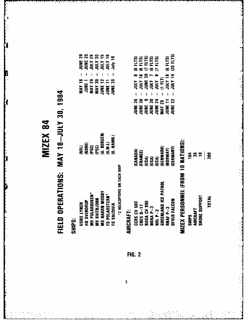
The 1984 Marginal Ice Zone Experiment (MIZEX 84), seeking to understandthe mesoscale processes that dictate the advance and retreat of the icemargin, was conducted in the Fram Strait area between Greenland and Svalbardduring the period 18 May to 30 July 1984. The culmination of over four yearsof planning and a continuation of summer MIZEX 83, this 1984 internationalArctic research program utilized the resources and expertise of ten nations.MIZEX 84 is the largest coordinated Arctic experiment conducted in themarginal ice zone and has the unique feature of an ad hoc organizationestablished by the scientists themselves without any intergovernmental agree-ments, memoranda or treaties. This has proved to be an effective scheme forplanning and conducting both MIZEX 83 and 84 field operations.

The MIZEX 84 experiment utilized seven ships, eight remote sensing/meteoro-logical aircraft and four helicopters, supporting a multidisciplinary teamof over 200 scientists and technicians plus ship and aircraft crews. Scien-tists, equipment and support came from Canada, Denmark, Federal Republic- ofGermany, Finland, France, Ireland, Norway, Sweden, United Kingdom arid UnitedStates. Figure 1 presents the MIZEX 84 platform and field organization.Figure 2 summarizes the participation for each platform.

The detailed schedule of operations for carrying out the MIZEX 84 experimentwas developed by the MIZEX Science Group over the past two years. Buildingon the MIZEX 83 experience, the operations plan with integrated schedule forall major programs was completed as planned with only minor field modifi-cations necessary. Figure 3 summarizes the MIZEX 84 experiment. In'formationon the individual MIZEX 84 project is presented by the Principal Investi-gators preliminary reports contained in this volume.

In preparation for the MIZEX 84 field operations, analysis of satelliteimagery was begun in Bergen on 1. May 1984. These data, coupled with theice reconnaissance flight by the Greenland Ice Patrol, provided the neces-sary information to select the final sites for instrumentation deployment.

USNS LYNCH began operations on 18 May 1984 by deploying an array of current

meters and an acoustic source in the open water areas of the Fram Strait.

An initial, open water CTD transect was also completed during the first legcruise by LYNCH.

POLARQUEEN was on station with all instrumentation deployed to start the DriftProgram on 8 June as scheduled. Wind and current drift carried her to theice edge and floe breakup forced a redeployment to the northwest on 17 Junewhere she drifted, moored to the same floe until the termination of thedrift experiment on 17 July.

Two synoptic CTD oceanographic mappings were completed. These included ex-tensive biological investigations. Mesoscale oceanographic investigations

I.

*along the ice edge included repeated studies of eddy features identifiedby the synoptic mappings and remote sensing overflights. The ability to re-ceive near real-time displays of mesoscale ice and water features from bothaircraft and satellite permitted the Field Coordination Team to prescribeship and aircraft investigation patterns. Three largescale CTD transects,including biological and ice stations, were completed across the Fram Strait.

The five-day synoptic meteorological experiment, 9 to 14 July, was an in-tensive study across the marginal ice zone. Four ships and several aircraft4participated in this experiment.Ice dynamics and ice physics studies were carried out by several coordi-nated and complementary projects aboard. POLARQUEEN, POLARSTERN andKVITBJORN including extensive tracking of an array of ARGOS drifting oceano-graphic-meteorological buoys and transponders. Near real-time analysis ofthese observations was also utilized in directing the experiment. Oceancurrent information was obtained by sub-surface drifters acousticallytracked (SOFAR), surface ARGOS buoys, CODAR, and current meters bothanchored and suspended from ice floes.

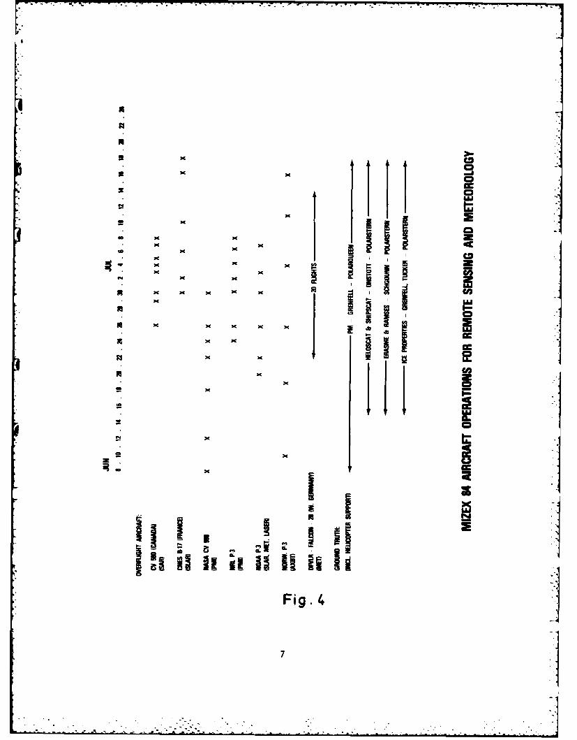
Extensive passive-active microwave remote sensing investigations were carriedout both by aircraft and in-situ platforms (see Figure 4). The observationsprovide synoptic characterizations of the marginal ice zone.

The acoustic program conducted, primarily from the Kvitbjern with vitalsupport from LYNCH, POLARQUEEN, SVERDRUP and P-3 aircraft from Norway andUSA, was carried out essentially in a single deployment between 9 and 29 June-

Some adjustment of the arrays were necessary near the end of the period asthe ice drift carried them near the edge where floe breakup began.

Modelers will utilize the data from many experiments to improve predictionsof the motion and behavior of the Arctic marginal ice.

*Fortunately, during the MIZEX 84 experiment, several low pressure systemspassed through the region. This resulted in variable wind conditions with

velocities ranging from 0 to 15 m/sec.

During June and early July flying weather was exceptionally good and heli-copters were able to fly to the limit of pilot times. In early June, one

* POLARQUEEN nelicopter had an engine failure while sitting on the ice. The

replacement engine was flown to the field, replaced and the helo was opera-tional tn just three days with only minor impact on project activities. OnePOLARSTERN helicopter suffered a rotor frame failure near the end of the

-* operations. This terminated the French low level scatterometer study ofthe ice surface. From the second week of July, fog prevailed thus limiting

* use of helicopters.

2

Ice floe ridging near POLARQUEEN caught one Bergen met-ocean buoy resultingin the loss of a string of six current meters and over a month of importantdata. However, one cyclesonde nearby was recovered by a diving team,SVERDRUP's experiment was terminated one day early due to an instrumentcable being damaged by a Russian ship.

Communications, usually difficult in such remote regions, proved to beeffective during MIZEX 84 in comparison to MIZEX 83 operations. The commu-nication plan, set forth in the Operations Plan, was modified twice tosimplify procedures and to minimize time spent in radio communication amongships and with shore coordination points. The use of telex and telefaxwere effective in reducing voice radio and for the relay of both data andfigures. The ability to use satellite telephone and telefax at high lati-tudes, up to about 80N, was and unexpected bonus for effective communi-cations. While more expemsive than radio, it did not interfer with instru-ments or data taking.

The Tromso Coordination Center was effective in scheduling aircraftoperations; in monitoring and relaying ARGOS buoy positions, near real-timeremote sensing analysis, weather forecasts, and ice conditions; and in avariety of logistic activities. High quality weather forecast were alsoprovided by the German meteorological office aboard POLARSTERN.

Completing essentially all the planned work as scheduled, every participantcontributed substantially to the success of the MIZEX 84 field operation.The combination and integration of these results should prove to be animportant advance in our understanding of the Arctic marginal ice zone.

I

3i

.a.In C,

I o-n 51j~

-z -a

5 a - , go a

9 _ _ _ _ _ _ _ _ P 2

LUA

.a C c

UU z ciC

am -A

va z M

a a'

aa 20

U, wJ

00 c

sa ai-

In CD z ID

am* a,Ie I

00

4L

Sc

cc -n -n - n Go- ~ ~ in i ~ i

-A -A-a- - _a -

66 A.LA-66 Li. LAGo toa

UU

a~ z

C% m~h r4 JO EC jC4

iui

= -,

LU I- ->-~~I C. .ac :

0. ci

* a a

~~ CDcnP. co ME cCcU =nw W6y~

CO)FIG 2 -.

LU C = C CC5

re 0

0

00

++

0 L

Q)V

0w 0

0 (D 0

04< w

-J - z 0 0 CDL . D~~~ I-J C- C j DlCd

crJ 0 a L 0S L) LL 0 -

S L L :E i : (CD - U L i . >-

LU or ~ CL I- LiM<: I 0 - 0 VLU C) LUw-J - z (2 0

L) 0 > > - M LiJ IZ LCL Ne V) -X J U L )

IN

NX

. CDCD

- xj

qD

LU

Fig. 4_i 1

*:N x

MIZEX CO-ORDINATTON TROMSO

Brian Farrelly9er'enIiX Group*, Geophysical Institute, University of Bergen, Norway

Tn romsoTX activity was concentrated at the MIZEX Coordination Center

at _rom-;o Satellite Telemetry Station. This center had four primary tasks:~mun: .. ,,on, buoy tracking, flight coordination and logistics. The center

was mannel by Brian Farrelly, Graham Symonds, Bob Shuchman and Imants Versnieks.

.onnunioat7-.os were based to a large extent on the use of telex for thetransm ssion o" Iaily routine messages to the ships. These messages included[ y ic'ily

weaitrnhe f'orecast prepared at the Weather Forecasting Center for Northern' borway,

report on aircraft activities,

• .i raft plans for next day,

ice edge information either using satellite images from Tromso Satellite.elemetry Station and S4R Nimbus 7 "real time" map, or based on telexesfrom Navoceano,

51 edited telemall or other messages to experimenters in the field..r uoy pos't',ns.

'Fter problems with long telexes buoy positions were sent separately.

h telexe- were prepared on an Osborne I microcomputer and transmittedto Rog'ala-.! R for retransmission to the ships. The conversion to telexeie use! a i -sler telex unit. After familiarisation with the equipment

tho setup worked well. It is understood that the ships at times had problemsr :each~n-T: !'an adio to sen-i and receive telex.

-elefax uslng satellite telephone was used to and from Polarstern for1 routine morning reports,

Ssketchmaps of SAR and SIAR results,

Sr)..R ice oharts based either on telemail from NASA Goddard Space FlightCenter or teleaxel maps from AES Associates, Canada.AXBT charts based on results from Norwegian P3 flights.

-he telefax link to Polarqueen over Svalbard Radio was tested successfullybut not used routinely.

.elephone over Svalbard radio was usel much less than in 1983 and only for*nonroutine traffic. Stellite telephone on Polarstern and Lynch workedextremely well andi was usable to much higher latitudes than in 1983. Thoughthis link is expensive the high quality enables traffic to be handled

* qui 1kly without repetition.

. Graham Symons kept track of the Argos buoys using an Osborne Executiveto access the telex files of System Argos in Toulouse via the Norwegianp Facket sentre network Datapak. This was done twice daily and the resulting* ,Rergen MIZEX Group: O.M. Johannessen, J.A. Johannessen, F. Svendsen,

* B. Farrelly, S. Sandven, T. Olaussen, S. Myking and A. Revheim.

8

.i .. .

diskettes were processed to reduce the data to a format suitable for trans-*' mission to the ships. Twelve hour mean positions were also calculated and-[ plotted on a large scale chart to obtain an overview of ice motion. The

task was time consuming and would have been impossible without the computer.

The Argos systemwas also accessed outside the routine times when necessaryfor buoy recovery etc. Buoy positions calculated using K. Aksnes (NorwegianDefence Research Establishment) algorithm in Tromso were alsoused for near real time (within/hour) updating. The Tromso positions arenow considerably more reliable tnan in 1983 owing to improvements in thealgorithm.

Wheras in 1983 southerly winds dominated and much of the ice motion waseasterly or northeasterly, northerly winds were experienced in 1984 leadingto southwards motion of the ice, with less coherence in the motion northof 80°N than in 1983. Further south the motion of the buoys showed theinfluence of eddies in the EGC and will be a valuable addition to CTD measure-ments. For more details see PI report from Graham Symonds and Ola M.Johannessen.

Bob Shuchman had primary responsibility for aircraft coordination. Thescientific objective of this coordination was to ensure that overflightsby remote sensing aircraft were supported by surface measurements, to achievenear simultaneous coverage by instruments requiring intercomparison, andto obtain optimal spatial and temporal coverage of the MIZ. The coordinationalso involved the safety aspects of ensueing adequate lateral, verticaland temporal separation of aircraft.

*Logistics were the primary responsibility of Imants Versnieks.

Finally an aspect of the coordination in Tromso was contact with the Weather- Forecasting Center for Northern Norway This was

not improved over the 1983 level. In addition the computer setup whichwas to be used for SMNR maps and digitising of weather charts at the Weather

Forecasting Center for Northern Norway did not work satisfactorily.

0

0•

0:

- . . .

I

OCEANOGRAPHY

4

4

4

I

11

4

OVERVIEW ON "POLARSTERN'S" ACTIVITIES

r Prof. Dr. Ernst Augsteiri

MIZEX was carried out during the second leg of "Polarstern's"1984 cruise Arktis II. On 12 June 1984 at 19.00 LT "Polarstern"left the port of Tromsb with 55 scientists and technicians and40 crew members on board.

rThe first task was to deploy five and to recover two deep seacurrent meter moorings in the sea ice covered ocean east ofGreenland at about 79°N. This work started on 14 June and was

- finished on 17 June. Both positions of the current meter mooringsK to be recovered were covered by large ice floes. Since the

mooring devices did not respond to the acoustic control thecommand for realease was given with some uncertainty. The firstone floated up in a small lead near the given position while thesecond one either did not react at all or was captured under theice. The mooring work was complemented by CTD measurements, seaice probing, biological and chemical analyses and meteorologicalsoundings.

On the way from the mooring site to the north" Polarstern" had ashort rendezvous with " Hakon Mosby" in order to exchangescientific gear. Both ships performed subsequently measurementswithin a so called synoptic grid accross the zonally oriented iceedge near 80°N. During this work "Polarstern" furthermorerecovered and redeployed two meteorological-oceanographic buoystations of the University of Bergen. Finally, the three meteoro-logical buoys of the University of Hamburg were deployed byhelicopter.

The synoptic CTD grid consisted of open water measurements by"Hakon Mosby" and stations in the ice conducted by "Polarstern"and helicopters. The extensive oceanographic survey was accom-panied by biological samplings, chemical analyses, meteorlogicalinvestigations, ice probing and remote sensing studies from theship and by helicopters. Because of heavy ice conditions the

*O synoptic work was extended to 22 June 09.00 GMT.

The following period from 22 to 25 June was primarily devoted to*- study the kinematics of the ice edge region in the area of the

first synoptic survey. A total of 10 transponders was distributedon ice floes by helicopters and tracked with the ship's radar.Seven transponders could be recovered, one was destroyed and twocould not be located. At the end of the minidrift station "Polarstern" met with the University of Hamburg's RV "Valdivia"near the ice edge in open water in order to assist in calibratingthe current measuring device CODAR.

When this procedure was finished both German ships started a

12

6

large scale oceanographic survey across Fram Strait. "Valdivia"was responsible for the open water part while "Polarstern"extended the first transect on 80°20'N through the sea ice west-wards to the East Greenland Shelf. A second transect wasexecuted on the latitude of 79°20'N. Heavy ice conditions forcedan extension of this work by nearly one day so that the beginningof the second minidrift had to be postponed until 06.00 GMT on 3July.

Due to this delay the full array of seven transponders and onereflector was operational not before the afternoon of 3 July. On4 July equipment and personnel of the Scott Polar ResearchInstitute was transferred to the RV "KvitbjZ5rn" in order tocontinue the transponder tracking from that platform. Three ofthe four Alfred Wegener Institute transponders have beenretrieved before "Polarstern" left the area on 4 July. During

* this experimental period some personnel was transferred from andto Longyearbyen.

For the second synoptic array "Polarstern" had to sail to 78°25'Nand 01°W. The survey was again carried out jointly with "HakonMosby" and "Valdivia". It ended at noon on 8 July when " Polar-stern" departed the area for the position further northwest whichshe had to occupy during the meteorological large scale network.

This position near 79°40'N and 60 30'W was kept from 9 to 14 July1984. Because of the relatively small water depth on the Green-land Shelf only reduced oceanographic and biological measurements

*have been conducted. Helicopter work was also considerablylimited since one aircraft was unservicable. Additionally, poorvisibility caused by fog forced the other helicopter also downfor most of the time.The large scale meteorological programme wasterminated on 14 July 12.00 GMT.

"Polarstern" then moved first eastwards to about 79045'N 2*30'Wand from there southeastwards to 79ON 00°30'E. On the entire lega total of 11 oceanographic stations some of which were extendedfor biological sampling have been carried out. The final obser-vational contribution to MIZEX was a meridional cross-section -

from 79°N to 78 0 20'N on the Greenwich meridian. The oceanographic* and biological measurements on this transect will help to

describe a relatively large eddy-like feature at the ice edge.

The ship departed from the experimental area on 17 July 16.00 GMTfor Longyearbyen/Svalbard where it arrived on 18 July 12.00 GMT.With the exeption of three persons all scientists and technicians

* disembarked during the afternoon of the same day.

13

PI REPORT, CTD GROUP, POLARSTERN

K.P.Koltermann, DHI, Hamburg

*." Euring MIZFX E4, Polarstern did 131 CTL casts, with ca. 1200 samples for

nutrients, oxygen and salt. lost CTF casts were run to the bottom, only31 were down to 6oo in. All standard cherical analyses were run on toard.

The CTr was C.016+/-0.003 to high compared to the salinity samIles runby P.Jores (IO).

K The stations worked during the cruise lej. can be grouyed into different

subsets

- a minifrid SSW of the Yermak Plateau- a drift station F of the Yermak Plateau with 25 hourly casts- five sections onto the Greenland Shelf along

78 25 N, 79 00 b, 79 20 N, 79 50 N and 80 20 N

* - one NYS section alone the Greenwich meridian between 79 and 7 N with

a 5 nm spacing.

Except for five casts, all were done in the ice.

The surface layers show strong features both horizontally and verticallymost can only be taken as meandering of the different water masses in or offthe ice edje.Only the holloy Ieep Eddy is persistent durine the whole cruise.lore detailed aspects can only be discussed after merginE the different CTDdata set6. The stronpestv variations are confined to tte top 150 r'. The under-lyinr Atlantic Water shows strone variations both in thickness, number of ex-trems and core temperatures, indicating especially east of the prime meridian

strong mixinc.

Along the Greenland Shelf the physical fields are much smoother and vary mainlyin EV direction. Here on the 1800 m isobath a very strone silicate raxirnum

in the surface layer is found, being evidence that the same feature observedin the Arctic,leaves at the west side of Fran Strait. Pelow the Arctic Inter-

Smediate Vater on the 2200 m isolath and at ca 1600 m depth a secondary silicatemaximum with hither salinities and temperatures sut-gests another deep outflow

from the Arctic, as also clearly shown in the 1'eteor data in 1982.

The Deep Water shows in Fram trait rather stron. horizontal chang'es both in

salinity, oxygen and temlerature, implyini° that within Fram 'Strait strong mix-* ing of waters of Arctic and Polar origin occurs even at depth. iollowinc in-

dividual irorerties in reslect to changes in tolpotrarhy one clearly notes thatall topographical chantes are reflected in the flow field at all depths. Thisstronely barotropic behaviour of the main circulation and the first order vari-ations have a significant influence on the distribution of properties near or

at the surface.

0

14

0

S

°N

' _ _ I a

tI I

I... ',

Si ,I

* I I _ _ _ _ _ _ _ _ _ _ _ _

i ::.- 1 I'r

I4D , ____ r/t V.

*1 - i

15

__i _ _ __1

I I I

* I I ,!

• - , |-I I o-

* oIi, " . i .' I'. - . . . . oI - . . " . _ .: . . . _ '

IzI

/" . . I

II

a) LI

_ _ I _ _ _ _- _

:1_ _ _ _ __ _ __ _ _ __ _ _ ___ __ _ __

1 1f16

£ I _ _ __

U. I

T~ .... * _ _ - __ _ _ __I

II

16 °

II

-c

C) CL

~ *7~v ~ a

0_ _ __ .__ _ _ _ _

r'. _ _ 1 _ _ _ _ _ _ . _ _ _ _ _ _ -

coA

* _ _ t 17

."

LAMONT CRUISE REPORT - MIZEX 84

Thomais X.inley

Lamont field operations were -onducted from the USNS LYNCH, the M/V

POLARQUEEN and the F/S POLARSTERN. During the May 18 to May 31 LYNCHcruise, a year-long mooring was recovered and one short term mooring wasdeployed. Both of the current meters in the long-term mooring succesfullyrecorded data over the complete period of 340 days at depths of 90 and 190meters. A 15-station CTD transect was also completed from the ice edge onto

* the Svalbard shelf at a latitude of 78 deg. 55 min. On the second leg ofthe LYNCH (5-22 June), which was primarily acoustics, a total of 11

additional CTD stations were taken during various cooperative ship programsEpertaining to MIZEX 84.

The helicopter-based CTD program was split between the POLARSTERN and thePOLARQUEEN. Observations commenced on the 14th of June and were concludedon the 17th of July. A total of 222 stations were taken during this time

period, ranging in depth from 100 to 650 meters, and as far away from the

ship as 50 nm. Of these, 208 were helicopter-based, and 14 provided inter-calibration statistics with the shipboard Neil-Browns.

Spatially, a majority of the helicopter-based CTD stations were confined

within the limits of 80 to 81 north latitude and 8 W to 10 E. Stations

outside this area were obtained primarily from the POLARSTERN in the regionfrom 79 N to 80 N and 2 W to 6 W in order to better define the East

Greenland front. Stations were normally grouped into single-day surveys

designed to accurately, as well as rapidly, map three-dimensional oceanic

structures from the extreme edges of the MIZ to the more centrally ice-covered regions. Patterns and interstation spacing varied depending on theinvolvment of open water, the proximity of ships doing CTD surveys to theice edge, and the type of feature being mapped. Most of these single-day

surveys consisted of four to ten stations set in either a linear or boxpattern with an average separation of 6 nm. Typical spatial average for abox survey was 150 sq.nm (depth of 600 m), while the largest 10-hour surveyaccomplished to date consisted of 14 stations and covered some 800 sq.nm.

Prior to completion of the field project, the short -term mooring previouslydeployed by the LYNCH was retrieved by the POLARQUEEN with all meters

functioning.

Over 60% of the helo-CTD data collected were devoted to cooperative mappingefforts with ship-based CTD's. Due to the dispersed nature of the data sets,it is virtually impossible to come up with explicit results. One survey,(which was predominantly helo-CTD oriented), however, did tend to indicatean intrusive tongue of warm saline water interior to the ice-edge front.

18

• °.

LONG-TERM CURRENT MOORINGS IN THE EAST GREENLAND CURRENT - EAST GREENLAND

POLAR FRONT SYSTEM

Robin D. Muench

Two long-term, over-winter current moorings were deployed approximately alongthe 1000 m isobath on the continental slope beneath the East GreenlandCurrent - East Greenland Polar Front system in mid-June 1984, early duringthe MIZEX East field program. Particulars, such as geographical coordinates,

I dates and water depths, are given in the below table. The moorings weredeployed from the vessel POLARSTERN by Mr. Clark Darnall of the University ofWashington (UW); no problems were encountered during deployment. The"standard" oceanographic taut-wire configuration was used. It is planned torecover the moorings sometime in summer 1985.

The MIZEX long-term moorings were deployed at the same time as a largerscale array across Fram Strait; the Fram Strait array was deployed as a partof Dr. K. Aagaard's (UW) program. At least three of the UW moorings will beused in conjunction with the MIZEX moorings to examine the mesoscale dynamicsof the East Greenland Current - East Greenland Polar Front system.Approximate locations for the MIZEX and three of the UV! moorings are shown,along with the local bathymetry, on the appended figure. Like the MIZEXmoorings, the UW moorings will be recovered in summer 1985.

Particulars for the MIZEX over-winter current moorings

Mooring Lat. (N) Long. (W) Deploy Deploy Bottom InstrumenLID Date (Z) Hour (Z) Depth (m)* Depths (,,">.

" MX-l 78043.988 ' 4051.131 ' 6/15/84 0846 994 94**394**

MX-2 78029.160 ' 4033.288' 6/15/84 0130 1020 120**420**

*Depths have been corrected for sound velocity variation.**Instruments were Aanderaa RCM-4 recording current meters.

19

I

19

4l

LONG-TERM CURRENT MOORINGS IN THE EAST GREENLAND CURRENT - EAST GREENLAND• ,POLAR FRONT SYSTEM

;* Robin D. Muench

0050 0

00 rV •MIZEXMOORING

0 0 u0 MOORING

00

790 A -790

0MX-1 0

MX-2

* 0 1000DEPTH IN NMETERS / km

0 50

Figure illustrating schematically the geographical locations of the MIZEXlong-term current moorings, three of the University of Washington (UW)moorings and the local bathymetry.

020

• -. ,.- • . .". 20

•01 .,: 1 : . . . . : . . _ : 1 _ . . . . . . . _ , , . _ . . .

Chemical Oceanography in the Greenland Sea

E.P. Jones and L.G. Anderson

The goals of the chemical oceanography program on board F.S. Polarsternduring MIZEX 94 were: (i) to examine the chemical composition of sea ice,(ii) to look for changes in the chemical constituents of near surfacewater as a result of the addition of sea ice meltwater and the presence ofsea ice, and (iii) to examine several chemical constituents of seawater forr. water mass identification and tracing.

In sea ice produced in the laboratory, the relative composition of salts inthe brine entrained in the ice changes as a result of the selectiveprecipitation of the salts from the brine when the ice is cooled. Calciumcarbonate is the first to precipitate, beginning to do so just below the

* freezing point near -2G.C, followed by sodium sulphate near -100C. Almost nostudies have been done to verify the laboratory results and their geophysicalimplications using sea ice produced under natural conditions. Several coresof first year and multi-year ice were collected throughout the MIZEX area.Not one showed anything like the degree of relative calcium enrichmentexpected on the basis of the laboratory results. Sulphate concentrationsq have not yet been determined, but based on the calcium data, little sulphate

enrichment is expected. These results seem to show that the studies of iceproduced under laboratory conditions cannot be used in any simple way todescribe the composition of natural sea ice.

The examination of near surface water to determine changes in compositionresulting from the addition of sea ice meltwater involved measurements ofcalcium, alkalinity, and 01/0 , isotope ratios. Preliminary results showessentially no change in either calcium or alkalinity attributable to thepresence of sea ice meltwater. Oxygen isotope ratios are expected todetermine how much of the freshwater component of the surface water is fromriver input and how much is from sea ice meltwater. 1Preliminary examination of the chemical data shows no obvious ice edgeeffects such as upwelling attributable to the physical presence of sea ice.Definite conclusions, however, will have to await a more thorough examinationof the data.

Water mass identification and tracing involves examination of salinity andtemperature distributions together with chemical components such as nutrients(measured by the University of Hamburg Chemistry Group), calcium, alkalinity,inoroanic carbon, oxygen, and pH. The chemical components are used bothindividually and in combination (e.g., nitrate and oxygen to form the tracer"NO") to determine circulation and mixing of water masses. The exploitationof these measurements will take considerable effort on the part of all groupscontributing to the data. One preliminary result immediately apparent,however, is the presence of water from the near surface halocline of theArctic Ocean identified by a nutrient and inorganic carbon maximum. Thiswater in the East Greenland Current seems to have maintained much of itsidentity along the Trans Polar Drift current and out of the Arctic Ocean

21

0

through Fram Strait.

Altogether, approximately 1500 samples from 90 stations were analyzed foroxygen and salinity, and approximately 800 samples from 50 stations for

*alkalinity, inorganic carbon, calcium, and pH. About 540 samples from 60stations were collected for oxygen isotope ratio determinations. Eight icecores, four first year and four multi-year, sectioned into 20 cm lengths,were analyzed for salinity, calcium, and alkalinity. About 140 samples from7 stations along the 820N transect and 12 samples at the western-most stationof the transect were collected respectively for tritium and helium-3analyses at the University of Miami.

0

S

"i 22

L

POLAR QUEEN Drift, MIZEX 84

Miles G. McPhee

During the main MIZEX 84 experiment, the POLAR QUEEN wasdesignated the primary drift-station vessel, and was allowed todrift passively with surrounding ice, while moored securely to afloe on which various experiments were deployed. The driftoccured in two phases: the first, which started about day 159.5(i.e., noon GMT on 7 Jun 84), was characterized by rapidsouthward motion in response to northerly winds. It wasterminated early on day 168 when ocean swell propagating in fromthe ice edge, which was by then about 1-2 km distant, broke thecamp floe into several pieces.

The ship and its surrounding instrument array were thenredeployed about 60 km to the northwest. The second driftstation was maintained for about 30 days, with the ship mooredto a large floe (approx. 300 x 400 m). Measurement programs

* were terminated at OOZ on day 200, with the remainder of theexperiment occupied by instrument recovery and transit.

Following are plots of navigational data for the POLAR QUEENduring its two drifts. Figure 1 shows each SATNAV satellite fixconsidered acceptable in the algorithm used by the Magnavoxsatellite navigator for updating its dead reckoning positions:this automatically disqualifies single channel fixes, low anglesatellite passes, etc., and appeared to have about the properselectivity. Acceptable fixes were randomly spaced in time,with typically 35 to 40 available per day. Crosses in thetrajectory mark the first good fix of each day. Times of thefirst and last fixes in each drift segment are listed.

In order to estimate drift velocity, the observed positions werefitted to a mathematical expression for position as a functionof time, which was then differentiated. The technique isdescribed in detail by McPhee (Drift Velocity during the

* Drift-Station Phase of MIZEX 83, MIZEX Bull. #4), and consistsof describing the trajectory as a superposition of mean driftplus clockwise and counterclockwise rotating components at twofrequencies: inertial (about 12.2 hour period) and diurnaltidal (24 hour period). Six complex coefficients were fittedevery three hours from all acceptable fixes in the preceding and

* succeeding 12 hours. The resulting coefficients were then usedto construct an evenly spaced time series of hourly positions, Iwhich are plotted in Figure 2. Here each dot represents theposition on the hour, with pluses indicating OOZ.

2I

23

Sq

From the fit coefficients it is also possible to construct atimes series of drift velocity as shown in Figures 3 and 4.Ordinate scales are cm/s. The designations 'east' and 'north'are approximate, being based on a coordinate system with they-axis directed north along the Greenwich Meridian (see thepositions plots); however, any correction is small, especiallyduring the second drift.

The final plot, Figure 5, shows ship heading as determined bythe inertial navigation every half hour, which data are usefulfor estimating floe rotation. Slop in the ship's mooring waspresent as mooring lines required adjustment, but was limite< toa few degrees.a

0 2 4 6 8

80.I I i , t -L...*,-e I. ..'-l........... i........ .F _. ... .. i -

4~. 80.6

I ~ ~ ~ ~ ~ ~ --i!I " ...-. e.

... . ........ . ...... 0. 3I ! . L . jI

i 0.2 ,•i I ... . I.-...-. 9...2

-I...." .-- -"-. 90.0

-i / ~I j. ii.--8.

----- ;I

POLAR QUEEN SRTNAV FIXES-- MIZEX 84

7 Figure 1

24

i.-" . .. ... , i .a

0 2 4 6B

--- - - - - -

-: I 3..2 80.2

I I

POLAR QUEEN DRIFT-- MIZEX 84

0 Figure 2.

40 1 1 1 1U V (North)20r'h

20

-20

160 170 18040 1 1 1 1 1 1 1

U (East)Eas 20

20

-20

-40160 170 IS0POLAR QUEEN DRIFT VELOCITY-- MIZEX 84

Figure 3.

25

40

26

-20

-46 1 1 1 1

166 196 200

40

-20

-40 1 1 1 1 1 1 1 1 1 1 1 1 1 1 1 1180 190 200POLAR QUEEN DRIFT VELOCITY- MIZEX 84

Figure 4.

360

320

240 ~

266

160

120

80

040. ..

160 170 180 ISO 200POLAR QUEEN HEADING- MIZEX 84

Figure 5.

26

LAGRANGIAN FLOATS EXPERIMENT

P.I.: J.C. GASCARD

The french program during MIZEX had two components:- remote-sensing of the marginal ice field using three active radars (Remote-

Sensing Laboratory In Toulouse/CNES)- Lagranglan observations in the Ocean and on the Ice (Physical Oceanography

Laboratory in Paris CNRS/MUSEUM).We report here on the second part of this program: Lagrangian observations, the purposeof which was to map the oceanic currents (mainly the Atlantic current) at surface and atdepth and the sea ice motions to get informations about variability and mean componentof motions and their dependance on atmospheric forcing, bottom topography, frontalstructures (3D) .

Three types of floats and buoys were launched depending on their use at surface or atdepth:at depth: 10 acoustic floats like SOFAR floats. They are freely drifting Swallow floatsballasted in order to be neutrally buoyant at preselected depths : 4 floats stabilizedaround 110 to 130 m depth and 6 around 200 to 260 m. The 10 floats were launchedfrom the POLARQUEEN (ship or helo) between 80014.4N - 80o43,5N and 3o30E -

6005. 5E from June 10 until June 20. Each float, equipped with a 1562 Hz transducer,sent a pulse every hour for tracking and was telemetering temperature and pressure insitu once every second day. Five listening stations received floats signals. and floatslocations were computed by considering time of arrival and position of listening stations.Three stations were operating In real time from three different ships: POLARQUEEN.POLARSTERN and KVITBJORN, and two autonomous listening stations. F1 and F2. weredeployed, at 700 m depth, from Ice floes tagged with Argos buoys and tracked bysatellite. Later on (post-MIZEX cruises), two listening stations were mounted first onPOLARSTERN (late July-early August) and later on LANCE (late August) extending thefloat tracking over a one month period In addition to the 50 days MIZEX period.

As a preliminary result, we can tell that we have been able to map some features ofAtlantic currents In the Fram Straits, below the Ice, during this summer 84 season: fourfeatures are already appearing related to the branching of the northward Atlantic currenttowards the southward East Greenland current:

- northward Atlantic current flowing along the continental slope West of Yermakplateau and entering In the Arctic basin.

- strong topographic features above Yermak plateau: one float has beentrapped during the whole MIZEX Experiment above the 500 m Isobaths Northwest ofSvalbard.

- recirculation of Atlantic waters west of the Yermak plateau along thecontinental slope and In the deepest part of the Straits.

- southward flowing Atlantic current trapped in the East Greenland current.

In addition to this experiment, we launched three VCMs (Vertical Current Meter) from theH. MOSBY close to the ice edge. Like the other floats, properly ballasted, they becomeneutrally buoyant at some depth. They are equipped with vanes around the main axis ofthe cylinder, 1. 5 m high. Then they rotate when drifting according to the verticalcomponent of motion (if any). We had a lot of trouble during this deployment for tworeasons: float depth equilibrium and listening equipment too sensitive according to shipnoise due to variable pitch. Nevertheless, after quite a bit of work, we succeeded In

27

- - . . . . . .. •.. .~

rdeploying two floats, at 200 and 700 m depth. In the Molloy deep area and one further

* Southwest along the ice edge. at about 78040N and lOW. Later on. we were not able to* recover the 700 m float because of a failure in the release mechanism. The float at 200

m. equipped with a SOFAR 1562 Hz acoustic (in addition to its proper 5 kHz short rangeacoustic tranducer) was tracked during 11 days above the Molloy deep. Launched on July4. 30 miles away from the Ice edge. at approximately 79o15N - 30E. It was recovered onJuly 15 by the KVITBJORN at about 79012N - 3030E. among thick ice floes. During these11 days. this float described an anticyclonic eddy trajectory with a 10 miles radius ofcurvature, more or less similar to the one described by the 700 m float. The third VCM.deployed along the Ice edge. followed a track parallel to the Ice edge during 2 days (July

* 10 to 12) at a depth around 125 m. It has been drifting Southwest at a mean speed of 20cm. s- 1 and was recovered at about 78035N - 2oW In loose Ice.

at surface: Other drifters were deployed, both on the Ice (7 drifters) and In the nearbyocean (7 drifters). They used Argos transmitter for location via satellite. Ocean driftersused temperature sensor for measuring sea surface temperature within 0. 10C accuracy.Initially. three of them were deployed In the Ocean. at the end of May from the LYNCH.two above the Molloy deep. at about 79020N - 30E. close to the Ice edge. and one Westof Svalbard. at 79oN - 80E. In the West SpItzbergen current. This last buoy remainedmore or less In the same area for almost the whole MIZEX period, going back and forth,North and South, and describing a lot of loops. At the end, It started drifting rapidlynorthwards and disappeared after passing by the Northwest corner of Svalbard. The two

* other floats remained in the Molloy deep area but did not last more than two weeks. EarlyJune, 4 buoys were deployed in the Ocean. two from KVITBJORN and two by helos fromPOLARQUEEN. few miles away from the ice edge. One of these failed rapidly for unknownreasons, two others, deployed from KVITBJORN at 80o20N-7oE and 80o30N-80E. lastedonly few weeks, while the last one Is still working after three months. On the average, ithas been drifting Southwest along the ice edge from about 79045N-70E (July 6) to74o45N -8o30W (September 18). During the first month, this buoy remained atapproximately 79o30N - 50E, trapped in eddy motions east of the Molloy Deep.

In summary. among the 7 drifters deployed In the Ocean (out of 10). three lasted for fewdays, two lasted for two weeks and two for respectively 2 and 3 months. We do not knowyet the reasons for such a discrepancy. It may be due to a mechanical failure of buoyswhen banging against Ice floes.

Seven Argos drifters were deployed on ice floes, In order to follow the drift of Ice stations:C2. C3. F1 and F2, and later on, at a currentmeter station with Bergen torold.which wasrecovered by POLARSTERN during post-Mizex. All these Argos buoys deployed on the icefloes worked perfectly during the whole MIZEX period. The recovery of these stations was

* not that simple and we are quite grateful to the pilots and chief scientists on POLARQUEENfor their patience and great help.

In conclusion, we are generally quite satisfied with our results considering our initial*planning. The SOFAR floats program has been accomplished to nearly 100% and we are

quite pleased with the offer of our German colleagues on board POLARSTERN and our* Norwegian colleagues on board LANCE for extending successfully the float tracking from

late July to late August. Due to the range limitation (100 miles) in sound propagation.related mainly to Ice coverage and bottom topography, we have not been able to receiveall signals from SOFAR floats at each listening station, but since our 5 stations wereredundant, we hope to recover most of the data for float tracking computations.

28

0•

. . " . .... . '~''~ 1 Ire Zone .x.erit. Io

Ir:cc:. It ,d ,: 1 '1:%, : the s,ac i l and temp -oral beha vi or of

i trt i:1 thno it ea , ciean in the marginal ice zone. For this,o i. nier li vertical profiles of temperature and salinity of the

1' or .2,,n '-m ::car thc ace to depths ranging from 50 to 1000 metersd 1: 1h t ttoe i:. t(va2 from 3 to 00 minutes using a Neil Brown CTD. In

idli t ion, we snSa ended an array of four Aanderaa current meters withtemrerature and c )nductivitv sensors from the ice floe to which Polar Queenwas moored in thne main halocline at a depth of 30 meters. The current meterarray was in the form w- a triangle with an interior meter slightly offcentf r resilting in hori.-ontal spacings ranginjg from about 100 to 400 meters.In urder to resolve internal waves adequately, the sampling rate was set atone sam: le per minute resulting in approximately 7-day long sampling periods.Two sets of data were obtained with this configuration. A single set ofdata was also obtained with the current meters suspended at 10, 40, 70 and100 meters from the ship adjacent to the CTD winch. In addition, weobtained in cooperation with the Lamont-Doherty and University of Washingtonqrours serial temperature and salinity profiles using CTD casts taken simul-taneously at three-minute intervals in a triangular array with spacings fromabout 100 to 300 meters.

As a service to the people studying the large-scale hydrography of theMIZEX region, we took routine CTD casts from the surface to near the bottomon a daily basis while Polar Queen was moored to the ice floe. In addition,we took special CTD casts with Niskin bottles for the University of Miamichemistry program and a number of special casts to 500 and 1000 meters tosupplement the Lamont-Doherty mesoscale helicopter CTD program.

Altogether we obtained 324 CTD profile records, 12 current meter records and19 timo-series of temperature and salinity. Preliminary processing of thecurrent meter tapes is being carried out at Lamont-Doherty GeologicalObservatory by Dr. Hunkins' group. The CTD tapes will be processed at theUniversity of California, Santa Cruz using a PDP11/34A computer.

Preliminary analysis of CTD profile series and time series of temperatureand salinity at fixed depths has shown that the principal internal wave

S activity was in the halocline at about 30 meters depth at a period of about7 minutes.

29

" .

;;7_ _ .__- __ - . . , . _• V__> •__ , -.: . - ---.

4

Cyclesonde Measurements in MIZEX 84

Dr. John C. Van Leer (University of Miami)

CAn array of Cyclesondes were deployed in the Fram Straits from the Polar

Queen during the MIZEX summer experiment during June and July 1984.

These instruments were launched from ice floes over the side using

timber "A" frames and a portable motor driven winch. The floe drift was

recorded by service ARGOS with French and Norwegian packages which

determine the position and provide reference velocity. Instruments and

mooring gear were transported by helicopter to floes 5-10km from the

Polar Queen. Data were recorded directly in each Cyclesonde on magnetic

tape and telemetered by radio to the ship and recorded by HP-86 on

magnetic disc. Cyclesondes were also deployed from the same floe to

which the Polar Queen was moored given by the A & B sites in the table.

The Cyclesondes recorded profiles of temperature, salinity, pressure,

current speed, and direction. Profiles were carried out at preset

intervals of 1/2 hour, 1 hour or every two hours. Most data were

sampled at 30 second intervals giving about three meter vertical

resolution. Some data were recorded at 10 second and 5 second intervals

for intensive periods increasing vertical resolution to 1 meter and 1/2

meter respectively. A summary of cyclesonde data appears in the table

below including an estimated 1,150 total profiles.

Instrument #71 was suspended from floe C1 when it was transformed into a0

pressure ridge on the 3rd of July. It was recovered on July 4th

still profiling under the pressure ridge with the aid of divers Tom

Grenfell and Don Perovich and a helicopter rescue effort directed by Jay

Ardai and Al Hielscher plus expert flying by Giles Porter of Luft

30

-7

Transport. The same instrument was redeployed on floe C2 which drifted

west across Fram Straits making hourly profiles. These data should

provide a unique record of the oceanic structure in the upper 200 meters

Iin the Fram Straits. The same helo team made a difficult recovery at

the end of the experiment at a range of about 75 miles in patchy fog.

In addition to temperature and current instrument #70 recorded light

" transmission data. Figures 1, 2 and 3 show respectively temperature,

u-component of velocity and light transmission in the upper 125 meters

of the water column. Niskin bottles, water samples and plankton hauls

4 were carried out at 35 and 60 meters at depths determined by local

maxiumum and minimum light transmission to see if these were caused by

specific organisms which might be used as water tracers for the flows

C above and below the thermocline respectively.

Technical support for both the mechanical and electronic sections of the

Cyclesonde gear were very capably provided by Mr. Larry Burton of the

University of Miami Ocean Technology Group at RSMAS. Computer support

was provided ashore by Mr. Peter Vertes (RSMAS programmer) and at sea by

0i Mr. Jay Villanueva a graduate student at RSMAS. Mr. Villanueva plans to

do a Ph.D. dissertation based upon the cyclesonde and other data

collected during MIZEX '84.

31

311

6!

TABLE OF CYCLESONDE DATA COLLECTED IN MIZEX '84

Tape Instr Launched Recovered Profiles Site Sample Profile# # Day/Hrs Day/Hr Recorded Ra te Interval

(Sec) (Hrs)1 71 165/19Z 167/14Z 12 A 30s lh

o 2 66 166/17 168/15 23 C3 30s lb

3 64 167/11 171/17 4 C3 30s lb

4 66 169/10* 174/10* 0 Cl 30s lh

5 71 170/12 170/21 0 B1 30s lb

6 64 173/10* 175/10* 0 B1 30s lh

7 71 174/11 178/5 91 Cl 30s lb

*8 70 177/14 178/16 3 B2 lOs Ih

9 64 178/9 181/7 4 Cl 30s 2h

10 19 175/10 184/6 172 BI 30s lb

11i 71 181/12 186/14 96 Cl 30s lb

12 70 182/14 187/15 82 B2 30s lb

13 64 187/13 196/12 52 Bi 30s lh

14 19 188/9 198/13 240 C3 30s lh

15 71 189/14 202/11 183 C2 303 lh

16 70 192/10 193/13 39 B2 los 0.5h

17 70 196/11 198/10 60 B2 los 0.5h

18 64 197/09 199/20 29 B1 5s 0.5h

19 70 198/13 199/19 60 B2 l0s 0.5h

0 1,150

0

32

0

m.

-M-4

LA DO 1 103 .- . .....

* U-)

>- ::, __ _ _ _ _ __ __3_ _

(ncn

U*) -

LIJ U)

C) m C

(.J.) CDE

24-)

LUJ 0 0

C))

Lii

LUn

Li

p... LJ L

*c U .LU - o

L-)J CL

LU 0 Z C*a,: I 0

ui C~icu .i.

CD ~Lni -

33

ARCTIC PROFILING SYSTEM OBSERVATIONS

Dr. James Morison

During MIZEX 84 we conducted an intensive study of the upper ocean at thePolar Queen drifting stations. A profiling current meter-CTD system calledthe Arctic Profiling System (APS) was used to measure profiles of tempera-ture, conductivity and horizontal velocity to depths down to 270 m.

Standard casts were made every three hours in order to monitor continuouslychanges in the mixed layer and upper ocean. Approximately ten sequencesof continuous profiles were performed. These ranged in length from 12 to24 hours. They were conducted during each storm to ensure high resolution

coverage of storm-induced transients and at other times to examine the*background internal wave field and other high frequency motions. A total of

1,082 APS casts were made in the course of MIZEX 84.

At the first drifting site we were able to make measurements during twostorms, including one during which the ice was swept out over warm water.The data from this period, combined with the turbulence measurements byMiles McPhee, should prove to be an excellent study of boundary layer andmixed layer dynamics under stable conditions. Strong near-inertial period

motions were also observed at this site. Experiments at the first siteended when the floe drifted out to the ice edge and broke up.

The second drift site was at a very large flow farther into the pack.Surface water temperatures were generally colder and we were able to studythe upper ocean response to ice motion for conditions which were not sohighly stratified. The longest continuous records were obtained at thesecond site.

3

Ii

I

I!

• 34 "

I.

POLAR QUEEN Turbulence Frame Experiment

Miles G. McPhee

The turbulence frame experiment for MIZEX 84 was designed tomeasure mean flow, temperature, conductivity, and turbulentfluctuations in the flow, at several levels in the upper oceanboundary layer beneath drifting ice. Special instrumentclusters were built consisting of three small (4-cm diameter),

S partially ducted rotors mounted along three mutually orthogonalaxes, plus Sea Bird conductivity meters and oceanographicthermometers. Data from each cluster were tranmitted to thesurface, converted to digital frequencies by a custom interfacedeck unit, and recorded on floppy disk with a Hewlett-Packardmicrocomputer. The system is capable of handling 7 clusters(35 data channels) at a sampling rate of 6 per second.

Clusters were mounted at various levels on a frame of stainlessrods bolted together and suspended through a hole in the seaice located some distance from the POLAR QUEEN. The computerand interface were housed near the main hydrohole in a heated

* tent shared with the University of Washington Mobile ArcticProfiling System (MAPS) project. Clusters were assembled in astandardized jig, and aligned carefully at deployment time withcarpenter levels. Each frame was weighted with ballast toensure that it remained near vertical.

CFor accurate current measurement, the system depends on currentshear between the sea ice and the upper ocean, since thecurrent meters have threshold velocities of about 1 cm/s headonto the instrument. Fortunately, MIZEX 84 saw a number offairly energetic drift events which developed well definedboundary layers near the ice/ocean interface. A real-timedisplay of the horizontal current vector at each level was usedto 'tune' the masts to an optimum orientation so that allcurrent meters in the cluster were turning at roughly equalrates. Coriolis turning in the boundary layer prompted use oftwo frames close together: one with shallow clusters(typically 1, 2, 4 m below the ice); the other with deep

• clusters (7, 15 m) usually oriented about 20-30 degreesclockwise from the shallower. On several occasions, thetemperature, conductivity, and horizontal currents werecompared with data from the MAPS, which uses similar sensors ina vertical profiling mode. These comparisons were usuallyquite close.

As described elsewhere in this report, the POLAR QUEENunderwent two separate drifts. Setup and initial testsoccupied most of the first drift; measurements were recordedfrom day 164 (12 Jun) to breakup on day 168. The mainturbulence frames (suspended through the same hydrohole with

* instruments at 1, 2, 4, 7, 15 m below the ice) were

35

re-established and recording at the second floe by day 174 (22Jun). A third frame with one cluster at 2 m below the ice,located about 100 m from the main site, was added on day 176.This basic configuration was maintained until the end of thesecond drift. A total of 205 hours of turbulence data sampled6 times per second were recorded during the project.

During the latter part of the second drift, the system was alsoused to test a prototype Diode Laser-Doppler Velocimeterdeveloped by Flow Industries, Inc. This instrument sampled twocomponents of flow by measuring Doppler shift of coherent lightscattered from microscopic particles in a small (order 1 cmdimension) volume. A special operating mode in the interfacedeck unit allowed sampling of the DLDV at 48 Hz, so that thehigh wave-number region of the turbulent spectrum could beinvestigated. The DLDV was mounted near one of the standard

turbulence clusters at 2 m on a separate frame for comparisonof lower wave-number response. A total of about 5 hours ofintercomparison runs were made.

Averaging and analysis routines were developed in the field fordata verification. Attached is a representative average whichshows perspective views of currents (averaged for about 5minutes) at 5 levels in the boundary layer. In the upperfigure, the horizontal components are shown as they weremeasured, i.e., relative to the drifting ice. Constructionlines for the horizontal vectors show the 'x' (eastward)component increasing with depth. Clockwise rotation withincreasing depth was present nearly all the time in themeasurements; exceptions being when the mixed layer deepened

past the instrument cluster at 17 m (15 m below the ice). Thishappened only once or twice; usually the salinity anddensity increased rapidly below 10-12 m, so that there was astrong pycnocline within the vertical domain of the clusterframe.

The lower view shows currents in a fixed-to-earth referenceframe, obtained by adding the ice-drift velocity to the

relative measurements. The remanent current at 15 m isprobably not due to surface stress, but is part of atime-varying baroclinic structure often present in thestratified fluid below the mixed layer.

Overall, the turbulence frame experiment appeared reasonablysuccessful. The data collection system and most of the sensorsperformed well. In both drifts, large variations in upper

* ocean temperature and stratification conditions wereencountered, which should provide insight into MIZ mixed layerdynamics not available before.

36

6L

ro -r---- -

N N1

IN

N-

41

37

a

TRITIUM LABORATORY FIELD OPERATIONS

Z. Top and H. Gote Ostlund

During the MIZEX 84 field work, our Further it was postulated thatobjectives were mainly to collect argon, krypton and xenon must besamples for the analyses of in excess of their respectivedissolved noble gases, oxygen saturation values. Oxygen is also

I isotopes, and tritium. In expected to be supersaturated dueaddition, we made dissolved oxygen to the freezing-melting cycle,measurements in the water column, however its production byon board M/V POLARQUEEN. phytoplankton and its consumption

by zooplankton makes the budgetingA total of 72 noble gas samples and calculations somewhat difficult.72 tritium samples were collected. With the present results we expectThese include detailed sampling for to confirm the anomalies and tonoble gases in the mixed layer (12 obtain correlations between them.samples in the upper 20 meters), 2) To obtain as detailed tritiumsurface tritium samples every other distribution as possible acrossday, ice core samples, and snow the Fram Strait. The temporal

* samples. Each noble gas sample variation of tritium in the highyields three aliquots; one for latitudes gives information a) onhelium 3/helium 4 isotopic ratio, the vertical mixing processes, b)one for the concentrations of total in conjunction with the oxygenhelium and neon, and one for the isotopes on the abundance and lifeconcentrations of argon, krypton time of the freshwater component

C and xenon. Samples for oxygen (Ostlund and Hut, 1984) and c) inisotope analyses are drawn from the conjunction with helium-3, on thetritium samples. The objectives of isolation time of a water parcelour field operations were achieved (time elapsed since last contactwith excellent cooperation of with the atmosphere).colleagues and the crew of the M/VPOLARQUEEN. Results of the The collected samples are expecteddissolved oxygen measurements were to arrive in Miami in mid-obtained on board, however these September, at which time they willwere further processed and are be processed and analyzed. Finalpresented in Figure 1. results should be available within

approximately nine months* The purposes for the above thenceforth.

mentioned measurements are asfollows: 1) To determine the References: .dissolved neon/helium ratios undersummer conditions. Previous Top, Z., W.B. Clarke, and R.M.measurements of neon and helium Moore. Anomalous neon-helium

* showed that there exists anomalous ratios in the Arctic Ocean. GRL,concentrations of neon in the 10(12), 1168-1171, December, 1983.Arctic regions, and the anomaly maybe explained by repetitive Ostlund, H.G. and G. Hut. Arcticfreezing-melting events (Top et Ocean Water Mass Balance fromal., 1983). Isotope Data. JGR, 89(C4), 6373-

* 6381, July 20, 1984.

38

6'

DISSOLVED OXYGEN9910 1 IQ 1%sat

r7.0 8.0 9.0 mI/I0 0 0

0000

* 2000A

0A0A

400 000

0 0AA000AA

600- 0A0A

*00 AA

E 0 A~800- 0 A

I0 A

F- 0A0- 0

wI1000-0 AO0 A

0 concentration1200 -oin mt/I

0A

1400- oA % saturation

*0 A

0A

1600- %o0A

00

1800

FIGURE 1. Dissolved oxygen profile in the Fram. Strait during* MIZEX 84 program.

39

4

MIZEY-84 OCEANOGRAPHY CRUISE REPORT, KVITBJ0RN (POLARQUEEN)

Einar SvendsenBergen MIZEX Group*, Geophysical Institute, University of Bergen, Norway

40 Aanderaa current meters distributed on 10 rigs, 3 automatic weatherstations and 3 thermistor chains were deployed (from Kvitbjorn and Polarqueen)anchored to ice floes. Some of these were tracked by radar transpondersin connection with the accoustic program (I. Dyer) and the minidrift program(P. Wadhams), the rest were tracked by Argos buoys. A total of 9 Bergen

- Argos buoys were deployed. Due to persisting northerly winds with equipmentdrifting out in open water and out of radar transponder range, most of thesites were redeployed at least twice. The current meter and thermistordata has not yet been processed.

In addition to the above mentioned activities, 327 CTD stations were takenfrom Kvitbjorn together with standard meteorological observations every10 minutes (wind velocity at 10 m height, air/sea temperature). Fig. 1shows the track of Kvitbjorn and the CTD sections taken. During the Kvitbjornaccoustic drift phase (June) and the two minidrift phases, CTD stationswere in general taken every hour to 500 meters depth. However, this time

* serie was broken up due to frequent redeployment work. In addition someshorter- periods of 3 minutes and 10 minutes CTD sampling to 100 meter depth wereperformed to look for internal high frequency waves. However, the main featuresseen were variations of isotherms and isohalines of 10-20 meters over 2-4 hourtime pericds. Together with the thermistor and current measurements every

2 minutes, and the acoustic program (I. Dyer), this will be an interestingdataset for the internal wave studies and its influence on acoustics.

- During the second phase (July) of Kvitbjorn (except for the minidrifts)the main CTD program comprised sections through eddies, some of these to-gether with R/V H~kon Mosby. With the aid of satellite and aircraft remotesensing, we were directed to areas where the ice edge configuration showedindications of' eddies. A section plot of isotherms through such an eddy

- is shown in Fig. 2. This shows that a patch of cold Arctic surface wateris moved far out from the ice edge, separated by warm Atlantic water inthe senter which is lifted to the surface.

Several of the current meter rigs (some equipped with ice ablation gear,0 E. Josberger) were for shorter periods at the very ice edge, and one rig

drifted into one of the eddies studied by CTD. Due to the frequent re-

deployment, most of the current meter data are of shorter time series,. however, they might prove to be very interesting datasets of features very

close to the ice edge.

Small scale ice rube melting experiments were successfully carried outluring instrument calibration periods.

*Bergen MIZEX Group: O.M. Johannessen, J.A. Johannessen, E. Svendsen, B.

* Farrelly, S. Sandven, T. Olar sen, S. Myking and A. Revheim.

40

- -S,. %

3- 2' Iw C' 'E 2- 3o 4. S' 6' 7' 8' 9' t0' 11"81,00.

9,6

28,6 21

3) 7 25)6 6/ 6,6

.,7 "6 C6 '6

2. 269)* 20)2

480*00 ', ~ ''*6 FRO- ONGYEAR ~6 2)

153 29)61600

0)7

3C5,

.7,.

258

%~~28 MIZEX 84 KVITBJORN327 314

2* %* .27 Positions 0500 GMT* '~~. C TO Sections

78*00' t i i i i i i i

Fig. i

44

w-

(L) ULgn f O-H - NGo

fNN

I0-2

0j

NI.,-

NN

0 J w

00C

N- 42

I

MIZEX OCEANOGRAPHY CRUISE REPORT FROM R/V HAKON MOSBY

,Johnny A.JohannessenBergen MIZEX Group*, Geophysical Institute, University of Bergen, Norway

This report includes the oceanography program carried out by the Univ. ofBergen group from the open water ship R/V HAkon Mosby during MIZEX 1984.The other main programs in meteorology, acoustic tracking of sofar/VCMfloats and whitecaps studies carried out from R/V HAkon Mosby are reportedby their respective PI's.

451 CTD stations were obtained in 53 CTD sections, 94 XBT's were droppedin 9 sections, surface temperature was continuously recorded with atowed thermistor and water samples were taken for deriving salinities.In addition Argos surface drifting buoys were recovered and redeployed

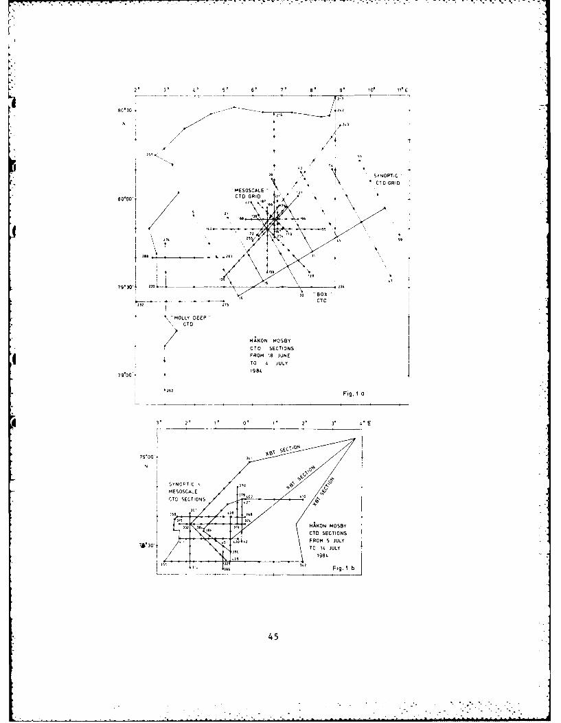
from R/V H~kon Mosby. The synoptic and mesoscale CTD programs includingstation numbers, section numbers, station spacing and sampling depthsare listed in the table below. The table also contains a listing of theXBT program. A map of the corresponding CTD section tracks are shownin Figure la and lb.

Preliminary analysis of this data set suggests that at least 3 differenteddy features were mapped. One eddy was detected during the first syn-optic CTD progsam with a center at approximately 79050' N and C 0 30'E.The diameter of this eddy was about 20-25 km. (Fig. 2). It was firsttracked for 4 days with CTD sections taken in a star pattern through theeddy center and revealed almost no propagation. At the same time the iceedge, initially located just north of the eddy center, moved northwardabout 60 km. The second tracking period 7 days later gave no sign of theeddy. This may imply a decay time in the order of 10 days.

Second, the existence of the "stationary" Molloy Deep eddy with a scaleof 60-100 km was revealed by 3 sections all sampled to the bottom.

Third6 eddy tracking with scales of 20-50 km along the ice edge southof 79 N was carried out in coordination with R/V Kvitbjorn. Location ofeddies by aircraft and satellite remote sensing in near real time en-able guidance of the ship towards the eddy feature.

In addition to the mesoscale eddy tracking program, the strong frontalzone between waters of Atlantic and Arctic origin in the Fram Straitwas mapped from R/ VHikon Mosby during the synoptic scale program byCTD stations and towed surface thermistor.

Both the mesoscale and synoptic scale oceanography prgram carried outfrom R/V HAkon Mosby wil contribute to the study and understanding of thelarge scale oceanography between Svalbard and Greenland.

Small scale ice cube melting experiments were successfully carried outduring instrument intercalibration periods.

* Bergen MIZEX Group: OM.Johannessen,J.A.Johannessen,E.Svendsen,

B.A.Farrelly,S.Sandven.T.Olaussen,S.Myking and. A.Revheim.

43

* .' ,,, ,..,.,L

E i E

c zi

- S * S +IS* - SS .. .

3

I

E E

- zz-zz - > . 7u : . ] ,!

zz z Z z . . . . .

' - . -" -- - . - : " - : - "- -' -- - C :,+= : - ?z,2.' "

. . . - 7 N C N . -7--

"" - - 5-z '

II

. -- - N C -,

-- '- S- -- . T -.,.. . 7 - 2 3

E E

i44

S. - •. -

7w.

2' 3. 46' 9 7o 8 91 101 1 E

80*30 --- ;6 , ANA

'9 SYNOPTIC

MESOSCALE \ /CYOGRID

80,00 CT GI

bb.

2'36

MOLLY BExCTOO

/ MAKON MOSBY

CTO SECTIONSFRM18JNTO 4 JULY

79*001984

233 Fig. I a

43 2 1 0. 1 2' 3' 4' E

N

CTO SECTIONSFROM 5 JUL.Y76' 30 TO 14 JULY

1984

32 Fig. I b

45

pop

-- -------- ----

I-ME B... . ,, 9 ._ --_

; . I g. 2. 2

r

a

'S. --- -' I

'"° <2 ,

Fi .

*4

a

, , ,, , ,.,., - .-.- , , .-... m i i -,- un il .- . hI

Hydrographic and current observations in the eastern Fram

Straits, RV VALDIVIA

r Detlef Quadfasel, Horst Baudner, Peter Damm and Klaus Schulze

Hydrographic observations have been made from aboard RV

VALDIVIA in the eastern part of Fram Straits during 22 June

to 18 July 1984 employing a CTD (ME-Multisonde) supplemented

by a 20 bottle rosette sampler. Station positions are shown

in Fig. 1. Current measurements were made in the West Spitz-

bergen Current by use of four satellite tracked drifting

C1" buoys.

1. Large scale2_roram: Three sections at 800 20'N (12 Stns),

at 78'55'N (15 Stns) and at 77'30'N (24 Stns) were occupied

between the ice edge and the coast of Svalbard. Additional

* 22 stations were run during the meteorological program in

the area of 78°N, 7*E (Fig. 1, heavy dots). All profiles

extend from the surface to 5 m above the bottom. XBT sections

were run on transit between CTD sections, station spacing

O varied between 3 and 10 nautical miles. (thin lines in Fig.1).

2. Sno12tic scale_2roramn: Four sections consisting of ten

CTD-stations each were occupied at 77 040'N, 770 55'N, 780 10'N

and 780 55'N (Fig. 1, crosses), spanning an area from the ice

edge to about 35 miles into the open water. Sampling depths

were 500 m and 1500 m alternatively.

3. Mesoscale 2ro2ram: Centered at 800 10'N, 30 E five sections

were occupied with a profile depth of 500 m (Fig. 1, light

dots). On their own probably not sufficient in coverage, these

sections were intended to support the intensive mesoscale

surveys of Hakon Mosby and Kvitbjorn.

S__4. Driftin2_ uo: Surface current measurements were obtained

from drifting buoys equipped with ARGOS transmitters. Three

were deployed on 780N at 20 miles spacing, one at 780 30'N

north of this row. The expected life-time of the buoys is

about 6 months.

47

6 t

w 0' E 0

80-N

7P N.

g Fig. 1: Hydrographic station Positions, VALDIVIA 21, MIZEX 84

* CTD 0-bottom (large scale)

+ CTD 0-500/1500 m (synoptic scale)

*CTD 0-500 m (mesoscale)

-XBT sections

A -------------- -------- IB --------C ----- I - -1

D -----------

23.6. 25.6. 30.6. 5.7. 1u.7. 15.7. 18.7.

* Fig. 2: VALDIVIA observational program

A: large scale

B: synoptic scale

C: mesoscale

* D: meteorological

48

I

Surface currents measured by means of CODAR

(H.-H. Essen

CODAR (Coustal Oceanic Dynamics Application Radar) measures

the radial component of surface currents up to a distance of

g50 km with a resolution of 1.2 km. Two measurements at

different positions are necessary in order to obtain the

2-dimensional current vector. During MIZEX, these measurements

" were performed successively, assuming the currents to be

( stationary for times of 1 to 2 hours.

A new system of receiving antennas on board VALDIVIA was tested

twice by means of correction (transmitting antenna on the

island Sylt and POLARSTERN, respectively). The angles of arrival

could be resolved unambiguously, but there is an inaccuracy

of t 15 in some angular ranges.

g Measurements of surface currents were carried out on 3

* sections between Svalbard and the ice edge (800 20'N,

780 55'N, 770 30'N). At the ice edge approximately 20 CODAR

stations were performed. The positions are shown in Fig.1.

*Two adjacent stations will yield one 2-dimensional current

map. In some cases, also three stations were taken to cover

the same area.

One CODAR station takes 18 minutes. During this time the

ship's course and speed should not vary. While the course

could be kept constant within t20, the ship's speed varied

up to t0,5 knots around 0. For this reason the processing

software has to be changed, which will take some time. We

hope to finish the data processing within 1 year.

49

V.. _ .... ...

I I.

I" Io'

I I

III

II

.1I

Sea Wave Measurements on Board MS "VALDIVIA" during MIZEX '84]

F. Ziemer Institut far Meereskunde, Hamburg, F.R.G.

1. Object in view and planning tant spatial distances in order to findout the spatial sea wave stimulation

The objects in view of part project ol/(fetch laws) as well as the influence3a of the MIZEX '84 exreriment concer- of the eventually existing ice bands.ning ms "VALDIVIA" are stipulated inthe additional motion of the SFB 94 of The conditions given by the planning ofOctober 4, 1983 and can be summarized the ship's time schedule permitted suchas follows: intensive sea wave measurement programs

only during the mesoscale measurementa) Measurements of the particular sur- phases. The estimated amount of timeface wave and current conditions pro- necessary for such a sea wave measure-duced by the ice edge; ment operation ranged between 12 and 14b) measurements of waves routinely hours, up to 8 stations included incarried through in order to set up a each operation, whereby measurementssmall scaled data set in a sea region had to be made in a distance of up towith scanty measurement points; 30 sm from the ice edge.c) further experience with modifiedship radar used for measurement of Regarding b):waves and current. Due to the large scaled operations be-

tween the ice edge and Svalbord and theRegarding a): 5-days meteorological measurement phaseThe main interest of the projected it was possible to effect routinely seameasurements concerned the specific wave measurements in a sea region, wherewaves conditions on the borders of the only a few data sets are disposed of.pack-ice. In cooperation with other Furthermore, these data can equally begroups doing measurements in the pack- used as reference data for measurementsice, it was intended to effect measure-made in the pack-ice as well as forments in distinguishing cases of two those made by plane.different directions of wind (on-ice-,off-ice winds). Due to the long time steps between the

stations, however, no stationarity ofIn the presence of on-ice winds the the sea wave field could be assumed. Onprocess of the reflection of sea wave the other hand, it was possible to re-and swell from ice edge back to the gister longer time series of the seaopen sea had to be registered at the wave development.same time as the process of attenuationof waves in the pack-ice. For that Regarding c):reason, it was intended to obtain on- Prior to the voyage the Furuno shipboard ms "VALDIVIA" sea wave direction radar had been modified in two points inspectra respectively the two-dimen- order to improve his suitability forsional sea wave spectra in short time measurements of sea wave and currents.intervals and in doubling space inter- First the pulse length had been reducedvals from the ice edge. by about 40% (to 38 x 10- sec) in order

to obtain a higher spatial solution,It was also intended to effect measure-necond the rotation amount of the an-ments in the presence of off-ice winds tenna had been reduced to 2 sec whichin rapid time intervals, but in cons- leads to a higher cut-off frequency of

51

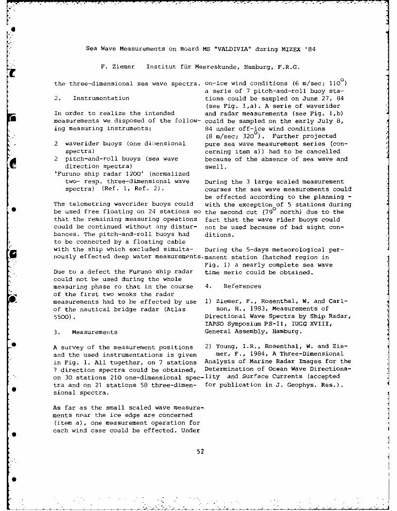
Sea Wave Measurements on Board MS "VALDIVIA" during MIZEX '84

F. Ziemer Institut fUr Meereskunde, Hamburg, F.R.G.

0the three-dimensional sea wave spectra. on-ice wind conditions (6 m/sec; 110

a serie of 7 pitch-and-roll buoy sta-2. Instrumentation tions could be sampled on June 27, 84

(see Fig. 1,a). A serie of waveriderIn order to realize the intended and radar measurements (see Fig. 1,b)measurements we disposed of the follow- could be sampled on the early July 8,ing measuring instruments: 84 under off-ice wind conditions

(8 m/sec; 3200). Further projected2 waverider buoys (one diniensional pure sea wave measurement series (con-

spectra) cerning item a)) had to be cancelled2 pitch-and-roll buoys (sea wave because of the absence of sea wave and

direction spectra) swell.'Furuno ship radar 1200' (normalized

two- resp. three-dimensional wave During the 3 large scaled measurementspectra) (Ref. 1, Ref. 2). courses the sea wave measurements could

be effected according to the planning -

The telemetring waverider buoys could with the exception of 5 stations during9 be used free floating on 24 stations so the second cut (79 north) due to the

that the remaining measuring opeations fact that the wave rider buoys couldcould be continued without any distur- not be used because of bad sight con-bances. The pitch-and-roll buoys had ditions.to be connected by a floating cable

* with the ship which excluded simulta- During the 5-days meteorological per-nously effected deep water measurements.manent station (hatched region in

Fig. 1) a nearly complete sea waveDue to a defect the Furuno ship radar time serie could be obtained.could not be used during the wholemeasuring phase so that in the course 4. Referencesof the first two weeks the radarmeasurements had to be effected by use 1) Ziemer, F., Rosenthal, W. and Carl-of the nautical bridge radar (Atlas son, H., 1983, Measurements of5500). Directional Wave Spectra by Ship Radar,

IAPSO Symposium PS-11, IUGG XVIII,

3. Measurements General Assembly, Hamburg.

A survey of the measurement positions 2) Young, I.R., Rosenthal, W. and Zie-

and the used instrumentations is given mer, F., 1984, A Three-Dimensional

in Fig. 1. All together, on 7 stations Analysis of Marine Radar Images for the7 direction spectra could be obtained, Determination of Ocean Wave Directiona-

*on 30 stations 210 one-dimensional spec-lity and Surface Currents (acceptedtra and on 21 stations 58 three-dimen- for publication in J. Geophys. Res.).sional spectra.

As far as the small scaled wave measure-ments near the ice edge are concerned(item a), one measurement operation foreach wind case could be effected. Under N

0

52

-

Sea Wave Measurements on Board MS "VALDIVIA" during MIZEX '84

F. Ziemer Institut fdr Meereskunde, Hamburg, F.R.G.

W 00 E

800N 800E1 ON

N80 N8 N.

NN

W 00 E l00

*Fig. I Positions of Sea Wave Measurements during MIZEX '84, VALDIVIA 21

waverider buoy

* waverider buoy and radar

x radar

1-4 pitch-and-roll buoy (7 stations)

waverider buoy and radar during the meteorological program

53

II

AXBT AND SONO BUOY DROPS FROM A ROYAL NORWEGIAN AIR FORCE P3

Ola M.Johannessen and B.A.Farrelly, Bergen MIZEX Group •

During MIZEX 84 6 dedicated MIZEX flights were carried out by a Norwegian

P3 from the 33 squadron at Andoya. 200 AXBT's and 19 sonobuoys for

ambient noise investigation were dropped in the MIZ. Fig. 1 shows the

position of the drops and Fig. 2 some preliminary results.

E.

II

6 * Bergen MIZEX Group: O.M.Johannessen, J.A.Johannessen, B.A.Farrelly,

E.Svendsen, S.Sandven, T.Olaussen. S.Myking and A.Revheim

54

I "I-6:

L"0

- -19 JUN, E 1984

. . . O_ 4, X° B, T ,Xf

S *? N N

* OA B T - e r

* OSONO !

2 0-

0 )6 JUNE-8..

6 0 0so 06000

120

jol,, "Do , ..

00

00

"o o0 '

0 0 _

0 2

-o/o .,_ .!~ 26.22 7

2* 0 2B AlBY

!~o • -E

-8 JULY 1984

°./

5- o NE 98C .. .

-'" Fig. I

* 0 0 0

550 " 16- - - - - . -; . .; ; . . . .i 2 i" ' ' "

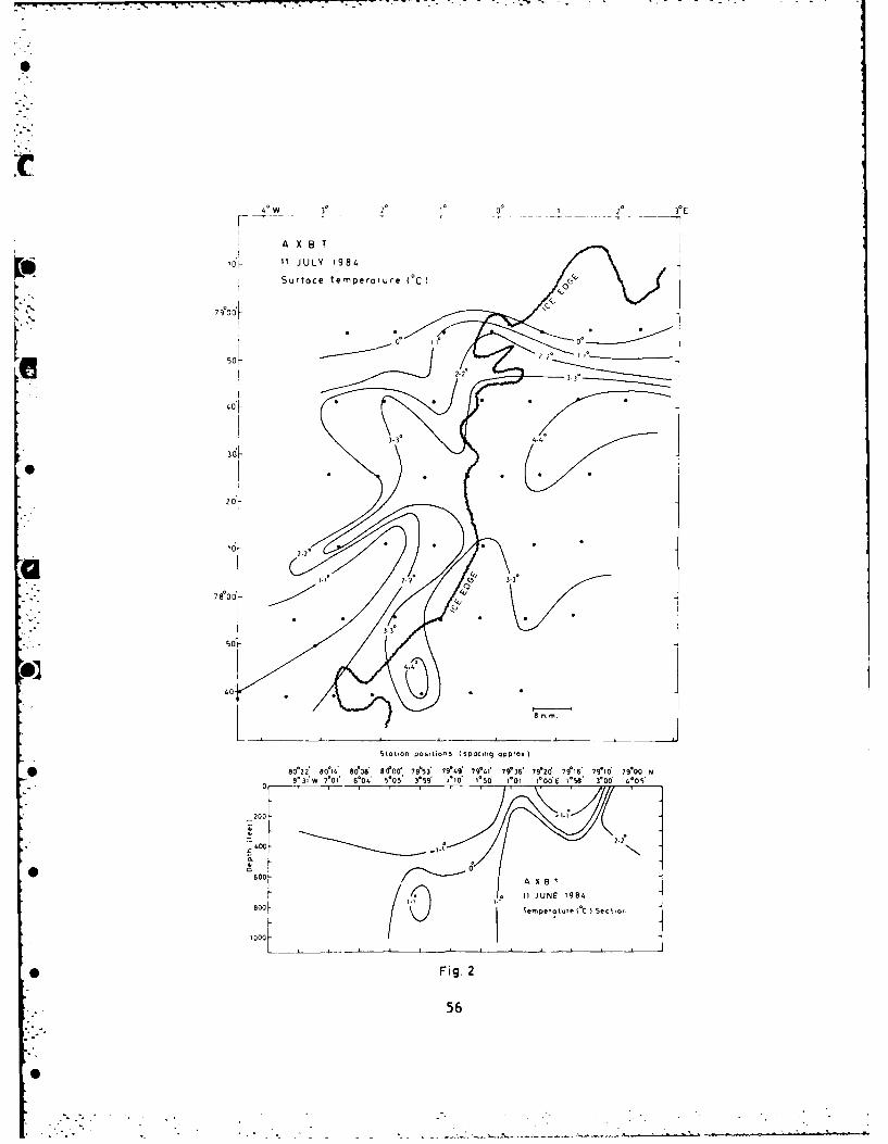
0R

3 -2 i~ ~ 1 2 f

700

26L

040

Statlon pos.1ions (spacing approx

80*22' 800. 8008' 8de0 79e53' W94 79P41' 7P36' 79F2d 79 6' 79 0 79!00 N*0~08* 31 W 7*01 6004' 5*05 3*59' o10* 150' 1*01 1*

00E 1*58 300' 4*05

_200 - -

2.2400 - .l

60 A X 8

11I JUNE 1984

800- '-)11 Terpe~aloe -C 1Set 1-

l000-

* Fig. 2

56

ICE

57

4

ICE RECONNAISSANCE BY THE DANISH METEOROLOGICAL INSTITUTE'S ICE PATROL

Ole Mygind

25/5 Departure cancelled owing to the weather in Narsarsuaq.

26/5 Departure from Narsarsuaq at 1440Z. Radar ice reconnaissance along the

west coast to north of Fredriksh~b, and directly to Sondre Stromfjord,

arrival at 1758Z.

27/5 Departure from Sondre Stromfjord at 0951Z, directly to Diskobay, and

then ice reconnaissance to Thule. The weather in Diskobay was bad, therewas limited visibility, mostly on radar. North of Umanaq-fjord it

cleared up, and the rest of the way to Thule the weather was fine.

4Arrival at 1416Z.28/5 Departure Thule at 1307Z. At departure the plane was filled up with

goods to Kap Moltke and Station Nord, mostly vegetables and post, and

"the important radio part" which turned out to be hi-fi equipment forStation Nord. The journey from Thule went past Herbert 0, through

Kane Basin, Kennedy Channel where we went to look at Hans 0, further

through Robson Chanal, and then along the north coast to Kap Morris

Jessup. The weather on the flight was nice, which also appears on the

ice charts. From Kap Morris the journey went directly to Kap Moltke,

where we, after a few overflights landed at 1817Z, and departed at

1917Z and arrival at Station Nord at 2018Z.

29/5 From Station Nord we departed at 1015Z. We flew directly to Henrik

Kroyers island, which, in spite of low clouds was found. There was

broken winter ice around the islands, and a thin layer of snow covered

the islands, no pressure ridges. From there we flew directly to the

observation area for MIZEX. The weather in the observation area was

6 very bad, low clouds all over the area, and foq over the ice, so the

visual observations were bad, even when the altutude was no more than

200 feet. The observation area was covered as suggested, ice charts

were drawn and a video-film recorded. From the observation area we

flew directly to Longyearbyen, arrival at 1500Z.

. 30/5 The communication was difficult, because the strike of the telephonecommunication personel in Norway was just finished, and it was

difficult to get the information about the weather in Greenland,

especially because the information was not requested in advance.

The meteorologist at the airport had to suffice the whole day, and the

* only information we got was that the weather was very bad at Mestersvig,

but later in the day it would clear up at Station Nord. At 1540Z we

departed from Longyearbyen with arrival at Station Nord at 1823Z

after a flight with heavy low clouds.

58

... . .- , . - . . - ..- .. -.. -

31/5 Departure from Station Nord was settled to 0800Z, but because oficing of the plane, the departure was delayed until it was cleaned.Mestersvig airport was closed because of water on the runway and badweather, so it was decided to go home via Thule and Sondre Stromfjord.We departed at 0935Z and flew directly to Thule, arrival at 1405Z.

After refuelling we departed for Thule at 1529Z to Sondre Stremfjordvia Upernavik, which expected ship arrival on 4-6. June. Icereconnaissance was sucessful as the weather was nice along the coast.Arrival in Sondre Stromfjord at 2019Z and after fuelling departure at4 2113Z, with arrival at Narsarsuaq at 2343A.

CONCLUS IONS

Because of the ice condition this time of year, it was too long tokeep the Twin Otter away from the primarily reconaisance area, andthere have been some complaints about this.

This time of year it is almost impossible to prepare flights over along period as the weather is very unstable, and the runway conditionsin North Greenland are dependent on the surface melt condition. Ifthe Meteorological Institute decides that the ice central should do( this kind of reconnaissance, we have to ask that a skilled person fromthe institution that wants the flying done, is present at the landingto judge the results, as it is not satisfactroy to do a job withoutknowing whether the intentions have been fulfilled.

59

I591

00

00

UJ00

00

k 0

0 0

00 A0

00

00

>6 00 0

0r

0 0

00

0

V 1-0

Go 4r

600

MESOSCALE ICE DRIFT FROM ARGOS BUOYS

eO.M.Johannessen and Brian A.Farrelly

MIzex Bergen Group *,Geophysical Institute,Univ. of Bergen

The MIZEX Bergen Group deployed 9 Argos tracked buoys during MIZEX 84.

Three of them T - T3, see Fig. I which shows the initial deployment, weretoroid<-s from whicg current meter rigs and meteorological sensors weredeployed. In addition T was equipped such that the current meter measure-ment were interfaced ani transmitted via the Argos system. The six remainingbuoys B 1 - B 6 reported position apart from B 4 which reported airtemperature and atmospheric pressure. B 4 was also equipped with currentmeters. Deployment commenced from R/V Polarqueen on 6 June and was completedon 8 June.

However, the predominantly northernly winds brought those buoys near theedge (TI, T2, T3 and Bl) so close to open water that they were at risk.Redeployment was therefore necessary and for T2, T3 and Bl repeated re-deployments proved necessary. Polarstern, Kvitbjorn and Haakon Mosby

assisted in these operation.

Those buoys together with the rest of the 45 or so Argos buoys deployed onice or as open ocean surface drifters were tracked at MIZEX CoordinationCenter, Tromso. Tapes containing the positions and data up to the end ofAugust have been received in Bergen and processing is planned to startshortly

S

0t

*MIZEX Bergen Group: O.M.Johannesson, J.A.Johannessen, E.Svendsen,2

P.Farrcelly, S.Sandven, T.0lausson, S.Myking and A.Revheim.

61

61I

.1

6]

- -*- ~ .*- .*~

00

0 E 20 40 60 80 10**82 000'IIII

N

0D B4 0D81 030' 0

F 2

B 5

81000' T 3 B2

00

T20 B

80030' [G

80000.

Figure 1

62

BEDFORD INSTITUTE OF OCEANOGRAPHY BUOY PROGRAM

G. Symonds

As part of the MIZEX 84 field program sea ice exiting through Fram Strait was"seeded" with satellite tracked buoys. The objective of this program was to

obtain estimates of the spatial and temporal variability of the mean and vari- 1ance of summer ice drift through Fram Strait. In addition three buoys wereequipped with anemometers to allow estimates of the wind driven component ofice drift to be made.

A summary of the data obtained is given in Table 1. At the beginning of the\1TZEX 84 field program six buoys were deployed across Fram Strait as shown inFigure 1. Approximately three weeks later a further four buoys were deployed

A. in the same geographic area. Deployment dates and positions are shown inTable 1. Two additional buoys were air dropped by the Norwegian Air Forceto extend the spatial coverage further to the west. However, both of thesebuoys failed to operate.

Except for the failure of the air dropped buoys and compass problems with oneanemometer buoy this experiment was successful with a total of 533 buoy days

* of data obtained as of September 15, 1984.

Shown in Figure I are the trajectories obtained from the first buoy deploy-ment for the month of June. The data shown in the figure represents aboutone quarter of the total data set. At the time of writing this summary theremaining data had not arrived from Service Argos.

Acknowledgements

I take this opportunity to express my thanks to M. McPhee and R. Lindsay onPolarqueen, E. Augstein and 0. Johannessen on Polarstern and the crew of theNorwegian P3 for deploying the buoys for me during the MIZEX program. Ialso express my thanks to the crew of Kvitbjorn who stayed and recovered twoof my buoys after everyone else had gone home.

630.

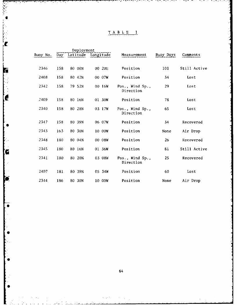
TABLE 1

DeploymentBuoy No. Day Latitude Longitude Measurement Buoy Days Comments

2346 158 80 0ON 00 20E Position 101 Still Active

2408 158 80 42N 00 07W Position 34 Lost

2342 158 79 52N 00 16W Pos., Wind Sp., 29 LostDirection

2409 158 80 16N 01 30W Position 78 Lost

2340 158 80 28N 03 17W Pos., Wind Sp., 65 LostDirection

2347 158 80 39N 06 07W Position 34 RecoveredO

2343 163 80 30N 10 00W Position None Air Drop

2348 180 80 04N 00 08W Position 26 Recovered

2345 180 80 16N 01 36W Position 81 Still Active

2341 180 80 20N 03 08W Pos., Wind Sp., 25 RecoveredDirection

2407 181 80 39N 05 34W Position 60 Lost

2344 186 80 30N 10 00W Position None Air Drop

64

S . , . . . , . . . . . . . . " '

1 h KX jIMf"- 0

kJ r

T2~K

Figur

c~. -65

MIZEX 84 MESOSCALE SEA ICE DYNAMICS: Post Operations Report

1 21W.D. Hibler III , M. Lepparanta , S. Decato K. Alverson1

1. USA CRREL, Hanover, NH 03755

2. Institute for Marine Research, Helsinki, Finland

This report summarizes the basic cha- addition, a variety of floe sizes and

racteristics of the mesoscale sea ice compactness conditions were sampled.dynamics data set taken from the Pol- Overall, the data set can be separat-

ar Queen, which was the main drifting ed into 3 phases (see Fig. 1). Phase

station during the MIZEX 84 experi- 1 covers the period 9 to 16 June,ment in the Fram Strait region. The during which the Polar Queen was

main purpose of this deformation ex- moored to a floe near the ice edge.

periment was to precisely measure This floe finally disintegrated on 16

mesoscale deformation and floe rota- June and the ship was moved to a

tion characteristics in order to larger, thicker floe further into the

learn more about the rheology and dy- pack, where it remained for the dura-namics of the interacting ice field tion of the experiment. During this

in the marginal sea ice zone. This first phase the ice was very mobile

can be accomplished by comparing the and dynamic, with substantial defor-fluctuation and rotation data with mation and drift occurring. This in

theoretical and numerical calcula- turn necessitated relocation of two* tions, and by using the deformation sites before the whole array was

data to verify more complete ice dy- brought in on 16 June. In particu-namics simulation models. lar, unit 72 was moved from site N3

to site N3B on 13 June, and unit 74The basic data set consists of pre- was moved from N1 to NIB on 14 June

cise (- I m relative accuracy) po- (see Fig. 3).sition measurements made at I5-minuteintervals of microwave transponders During the second phase of the exper-

* located at as many as five sites from iment from 17 June to about 6 July2 to 18 km from the ship. The angles the ice was much more compact, and

are determined less accurately by the deformation, except for relative-

triangulation. Data acquisition was ly major deformation events every

automated with an Apple I computer week or so was much less pronounced.

programmed up to automatically ac- During this phase the ice was mostly

quire data via a communications line "locked together," with smaller fluc-

connected to two master ranging units tuations occurring. Three transpond-

on the flying bridge. These data ers had to be redeployed in thiswere printed and recorded on magnetic phase, mainly due to intense ice

* disc at 15-minute intervals. In ad- ridging which occurred on 3 July at* dition, during most of the experiment site Cl where two transponders were

the rotation of at least one of the located. This deformation destroyedfloes supporting a transponder was two tripods, knocked one of the units

monitored at 15-minute intervals by into the water, and bent an antennausing two transponders about 50 m a- on another. However, after being re-

* part on that floe. Because of the covered the Del Norte transpondersdifferent locations and drift of the were found to still work fine, andPolar Queen, the data set is particu- were moved to new, separate sites (N3

larly complete, and comprises over 30 and CIA). The transponder at NI was

days of deformation data acquired also moved to N4 on 4 July to obtain

both in the interior of the marginal a better areal coverage.

* ice zone and near the ice edge. In

66

09

Toward the end of this second phase proved most durable and was found to

the deformation began to pick up as be very easy to relocate, as it could

the ice became less compact. As a easily be slung fully assembled by

consequence, most of the units final- helicopter. Oversized batteries con-

ly drifted out of range and the whole tained in insulated wooden crates and

array was redeployed on 12 July as a quick battery disconnects were used

3-site array with two transponders at to power the units. They were left

two floe locations for more complete up to 9 days at sites without ranging

floe rotation measurements. This ar- failure. The only man-made problem

ray too rapidly diverged until it was encountered was a bad battery connec-

* picked up on 16 July with some of the tion at the slave site, which pre-

units out of triangulation range. vented triangulation data from beingobtained for about 1-1/2 days during

To make distance measurements with the second phase. The other problems

this transponder system, the distan- were drifting out of range, bear at-

ces to a site from the ship and from tacks on equipment, and ridging. Al-

. a "slave" triangulation site located though floes did break apart, this

at one of the transponder sites were did not affect any transponders.

simultaneously measured. This infor-

mation alone allows the x-y positions Fig. I presents an overall chart of

of the array in a rotating coordinate data taken and is organized by trans-

system to be determined and, hence, ponder unit number. In the table, RL

* the strain rate invariants to be de- refers to a "range loop" measurement

termined with considerable accuracy. which essentially gives the distance

To locate the orientation of the ar- from the "slave" site. Gaps (other

ray in absolute space, angular mea- than occasional one- or two-reading

surements to a passive radar trans- data dropouts) are indicated but not

ponder at the slave site were made at annotated with details (bears, defor-

8-hour intervals using the ship's ra- mation, out of range, etc.). Site

dar. coding is noted and can be comparedto the scale drawings of transponder

A particularly valuable feature of locations at various times throughout

this array is that it can be ranged the experiment in Fig. 3.

from using a helicopter-mounted mas-

ter unit. By using an inverter to To give a feeling for the actual time

run an HP computer which in turn con- series data required, Fig. 4 shows a

trolled a master ranging unit in the time series plot (on the Apple print-

helicopter, it was possible to "home" er) of distance to unit 86 at the end

in on the radar transponder and re- of phase 2 and beginning of phase 3.

trieve It after it had drifted either The later high deformation shown is

* out of range or at least out of tri- very similar to that experienced dur-

angulation range. This was effec- ing phase 1.

tively used at the end of phases 2

and 3 to retrieve units which other- Overall it is felt that this data set

wise might well have been lost. Amaz- represents a unique set of measure-

ingly enough, despite the very dynam- ments of the deformation field of a

* ic deformation conditions, no equip- series of interacting ice floes. Be-

ment was lost during this experiment, cause of the fine temporal resolu-tion, accuracy of the measurements,

The actual mounting of the transpond- and coincidence of current and wind

ers on the ice made use of a collaps- measurements, these data should great-

ible tripod system designed by Dave ly aid in understanding the physics

* Fisk of CRREL (see Fig. 2). This of marginal ice zone dynamics.

67

I

_]

Transponder Number

72 12RL 74 74RL 76 76RL 82** 82RL 84 84RL 86 86RL

TF 1 N3 NI N2 C3 -• C2 C2

13 I I 1 1 1r--I CI C3 -

16 I T I I

C 12 • NI1820

"-L N- I_2_1

29T N2

.CIA -- :

4N4

I j IIo.. .. .. II L I iI I

* 16,* * T*ongulahon Site 3 Transponders Being Triangulated

Figure 1. Deployment chart for transponders. The chart shows timeswhen direct measurements and range loop measurements (denoted by RL)were made at 15-min intervals to transponder unit numbers 72, 74, 76

and 82, 84, 86. For range loop measurements, a slave unit was lo-cated at site 82. (The range loop measurement to 82 is redundant as

it effectively gives an additional but unneeded distance measurementto unit 82 from the ship.) Also denoted on the chart is the loca-tion of the unit with reference to Fig. 3.

*I

S" -Figure 2. Transponder tripod fullydeployed. This picture was taken by

Buddy Mockford on 29 June after unit

76 was deployed at site N2. Forscale, Bill Hibler, on the right, is6'6" (1.98 m) tall and Steve Decato,

* on the left, is 5'8" tall.

68

* Transponder N C2

(+) Polarqueen 14

24 June

22 July

N

+ +3 NN C

+C2

N3

C2 3

NCll

12 July+ C3 **RI

CIAN4. N39 C3

R2

N2.

Figure 3. Scale drawings of the array configuration at representative tiUesthroughout the experiment.

14X200- I 'I I ' ' I I I

E 12 -

S10OE 8 .-

- --

024 6 12 18 24 6 12 18 24 6 12 18

* 7 Jul 8 Jul 9 Jul

Figure 4. Time series of distance measurements to unit 86 located at siteN4. The resolution here (40 m) is dictated by the printer used for the plot.The actual distance measurements are accurate to I m and are recorded to thenearest 0.1 m. Distances are plotted modulo 3000 m. The initial distancewas slightly greater than 6000 m.

69

" -".I." '.. ' I

SCOTT POLAR RESEARCH INSTITUTE PROGRAMME ON ICE EDGE KINEMATICS, WAVES ANDAERIAL PHOTOGRAPHY DURING MIZEX-84

P. Wadhams, V.A. Squire and A.M. Cowan

1. Ice edge kinematics. The motion and deformation of the ice cover near themargin were measured during three "minidrift" experiments, in which arrays ofradar transponders were tracked from ships. The first minidrift was carried outfrom "Polarstern" during June 22-25. The ship positioned herself at 80 0 14'N,

* 3 0 E, about 8 n ml from a diffuse ice edge and close to two Bergen toroid buoys(5062, 5064) equipped with weather stations and current meters at 5, 10 and 40 mdepth. Four SPRI buoy sites were set out, each site comprising a radartransponder and reflector, a "Seadisc" one-dimensional teleretering wave buoyand an Aanderaa current meter at 10 m depth. At the same time 6 radar-radiobuoys were set out in the ice edge region (1-2 n ml from edge) in a jointprogramme with H. Ito (Alfred-Wegener-Institute) to study extreme edge phenomenasuch as longshore jets. The arrays were tracked for 3 days, with remote sensingcoverage via helicopter photography (A M Cowan), CV990, NOAA P-3 and Falcon

'd overflights. On the second day the wind direction changed radically from off-E ice (N) to on-ice (SE). The drift direction of the array changed to keep themean drift at about 400 to the right of the wind, but also the ice edge becamemore compacted with the array flattening along an axis at right angles to theice edge and stretching in the along-edge direction. After compaction, thewhole array gradually approached the ice edge, the rate of approach being ameasure of the lateral erosion of the edge from wave-induced breakup and melting

The second minidrift began from "Polarstern" early on July 3 and ended from"Kvitbjdrn" late on July 7. "Polarstern" began her drift at 80 0 26'N, 1 0 20'E,some 15 n ml inside the ice edge and 15 n ml from "Polar Queen". The aim was tocouple the ice edge array to "Polar Queen's" interior array, with onetransponder being tracked from both ships. An array of 4 SPRI buoys and 4 Itobuoys was set out. The ice edge was compact, with some vast floes near the

I edge, and with a possible eddy feature comprising a deep inlet extending severalmiles into the ice (investigated with CTD surveys by "Valdivia" and"Kvitbj~rn"). The two Bergen toroids were deployed by "Kvitbjlrn" close to thearray, to provide additional wind and ice-water velocity field data. The arraymoved southward initially, with some anticyclonic rotation and a stretching asthe buoys furthest to the S and W began to experience a strong ice edge jetrunning to the SW. Late on July 4 "Kvitbjdrn" moored to a floe near"Polarstern" and deployed a meteorological mast and tethersonde (BIO and AES)."Polarstern" then transferred SPRI personnel (except Cowan) and, after recoveryof Ito buoys, the tracking of the SPRI array continued from "Kvitbjorn". Afteranother 20 hrs of southward drift, the array, now close to the ice edge, beganto move rapidly to the SW, driven by the ice edge current jet and a N wind.During the next 48 hours the array drifted 32 n ml ending at about 790 50'N, 10 W.Little further rotation or deformation occurred during this period. Recovery of

_ the array took place late on July 7. Remote sensing coverage during the driftcame from helicopter photography (from "Polarstern" and "Polar Queen") and theNOAA P-3.

The third minidrift took place from 17-21 July, on the south side of theprominent ice tongue associated with the semi-permanent Fram Strait eddy."Kvitbj~rn" set out 3 SPRI buoys then positioned herself at 79 0 09'NWO°W to begin

* tracking. A fourth buoy was set out on the following day. Fig. 1 shows thedrift and deformation of the first 3 buoys. Iitially this consisted of pureanticyclonic rotation at a rate of 1.4 rad day-, a measure of the vorticity ofthe eddy itself. Then the rotation slowed and the array moved SE, flatteningitself out along the ice edge: the entire eddy appears to have changed shape sothat the array drifted into a region where it was more affected by the normaldrift of the East Greenland Current and less by the eddy vorticity. Furtherinterpretation awaits analysis of satellite and aerial imagery. Two of the SPRI

70

0,

buoys were set up beside Bergen toroids, equipped as before. Aerial photographyof the array was provided by "Polar Queen's" helicopter; recovery after 3 dayswas done by ship.

2. Waves programme. The waves programme was designed to measure the directionalwave spectrum inside and outside the ice edge, so as to determine the effects ofreflection and refraction as well as attenuation. During June 16 to July 2, 16stations were occupied from "Polarstern", comprising a 5-station helicopter"floe hopping" experiment, where a heave-tilt sensor was deployed on floes at 10km intervals along a line moving into the ice; and 11 single stations using theheave-tilt sensor, a Seadisc or an Endeco Wavetrack directional wave buoy, tosupport remote sensing overflights or open water stations carried out by"Valdivia". From July 4 onwards a more concentrated programme from "KvitbjQrn",carried out in co-operation with Institute of Oceanographic Sciences (R.

* .Pascal), involved some 60 stations using the IOS pitch-roll buoy, the Endeco andthe heave-tilt sensor. A typical line of stations would comprise buoydeployments at 10, 5, 2, 1, 1/2 and 0 n.ml. outside the ice edge followed byheave-tilt stations on floes as deeply into the ice as "Kvitbjdrn" couldpenetrate. 5 lines of this type were done. In addition 2 band experiments weredone, in which buoys were deployed to windward, leeward and beside prominent iceedge bands, to study the effect of wave radiation pressure on band dynamics.

In an associated programme, E. Josberger (USGS) deployed sensors to measurebottom ablation and wave-induced sidewall ablation of floes. To measure themodification of the upper ocean structure associated with the resultingmeltwater, S. O'Farrell (SPRI) operated a mini-CTD from floe edges and in leads

* (using "Kvitbj~rn's" motorboat), down to 80 m depth.

3. Aerial photography programme. The SPRI Vinten F95 reconnaissance camera wasused in conjunction with video filming to obtain a total of sixteen aerialphotographic datasets in support of various experimental programmes. In sumapproximately 5000 frames of vertical photography are suitable for analysis.

42 The list that follows indicates the purpose of each dataset:

Video 1 14 June ice reconnaissance supportVinten 1, Video 2 15 June as aboveVinten 2, Video 3 15 June wave attenuation experiment I

Vinten 3, Video 4 17 June " " " 2Video 5 18 June CV990 overflight support, re: radar altimeterVinten 4, Video 7 22 June scatterometer support, re: R. OnstottVinten 5 22 June as aboveVinten 6 23 June first mini-drift transponder array overflightVinten 7 23 June ice edge to ship, re: floe size distributionVinten 8, Video 9 24 June mini-drift transponder array overflightVinten 9, Video 11 28 June CV990 and scatterometer supportVinten 10, Video 12 30 June CV990 supportVinten 11, Video 12+13 2 July Fram Strait eddy transectsVinten 12 3 July second mini-drift transponder array overflightVinten 13 4 July as aboveVinten 14 4 July as aboveVinten 15 9 July scatterometer support and SAR-580 supportVinten 16 13 July intensive aerial coverage of 5 x 5 n ml box

forward of Polarstern for surface roughness* measurements re: meteorology of boundary layer

(C. Wamser)

The statistical analysis of the above datasets involves all two-dimensionalgeometric properties of the ice cover so as to yield, e.g. concentration, floesize distribution, etc. Surface roughness estimates may be made with referenceto supporting surface photography.

0

71

0"

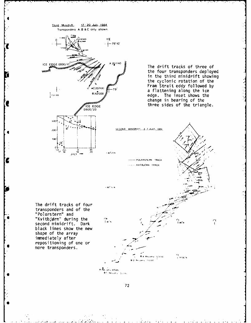
Third Minidrit. 17-20 July. 1984

Transponders A, B & C only shown

0.Io.oo 1 E

+79'10

ICE EDGE 0017AN14A 2"/-40 The drift tracks of three of

the four transponders deployed-, "in the third minidrift showing

the cyclonic rotation of theFram Strait eddy followed by

*C 2011100 a flattening along the ice1,m B0 edge. The inset shows the

change in bearing of theICE EDGE three sides of the triangle.

0800 /20

3001

200 SECOND MINIDRIFT 37 JULY 984

100 I

V718 19 20 bO', N"

.............. POLARSTERN TRACK

KVITBJORN TRACK "-

The drift tracks of four -'

transponders and of the"Polarstern" and -'

* "Kvitbjorn" during the '0 0' -- '"0 1- E 2

second minidrift. Dark N , . . iblack lines show the newshape of the arrayimmediately after .. '.- . "repositioning of one ormore transponders. '"

A Fl-,, I!/22 30 750 N

- *~0 H " '.,'72

72

S'

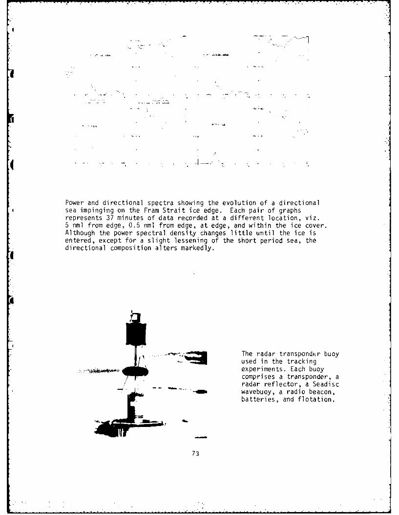
Power and directional spectra showing the evolution of a directionalsea impinging on the Fram Strait ice edge. Each pair of graphsrepresents 37 minutes of data recorded at a different location, viz.5 nml from edge, 0.5 nml from edge, at edge, and within the ice cover.Although the power spectral density changes little until the ice isentered, except for a slight lessening of the short period sea, thedirectional composition alters markedly.

r- ........ .. : The radar transponde.r buoy...... -. used in the tracking

• . . . experiments. Each buoycomprises a transponder, a

/ ' radar reflector, a SeadiscSwavebuoy, a radio beacon,

batteries, and flotation.

AMLA

73

4A . - - .

.

Extreme Ice Edge Ablation Studies

Edward G. Josberger, U.S. Geological Survey

The extreme ice edge ablation studies took place during the second portionof MIZEX 84, 3 to 20 July 1984, the instrumentation deployed from Kvitbjorn.The goals of the program were to measure the bottom ablation in coordinationwith the ice-edge phenomena study and to measure the wave field in the leadsas it relates to waterline ablation. A complete understanding of the bottomablation requires the melding of this data set with the current-metermeasurements made at each toroid site by the Geophysical Institute,University of Bergen.

On 3 July 84 during the 2d minidrift USGS deployed 3 acoustic bottomablation gauges, one at each of the 3 Toroids deployed by the GeophysicalInstitute. When Kvitbjorn took over the minidrift from Polarstern, USGSdeployed an acoustic bottom ablation gauge, and one current meter 7m belowthe ice at the center of the drift site. Also, periodically during thedrift phase, a capacitance wire wave gauge measured the shortwaves in theadjacent leads.

On 7 July Kvitbjorn recovered all of this instrumentation. The bottomablation records show little melting for the first fwo days but for thelatter two days the melt was approximately 10-20 cm day- . The increase inablation resulted from the ice drifting into warmer water which was shown bythe CTD costs throughout the period.

During the ice edge phenomena study from 9 July to 13 July a bottom ablationgauge was deployed in conjunction with a Geophysical Institute toroid andcurrent meters in an ice tongue. The Toroid was recovered on 13 Julyfloating free in scattered ice. The ablation record showed that the ice hadmelted by about 40 cm before breaking up. The floe broke up approximately24 hrs before recovery. During this phase periodic wave measurements weremade.

For the 3d minidrift, 17-20 July, bottom ablation was measured at the twoToroids and at the drift site. Also at the central drift site, a currentmeter was deployed at 5 m below the ice and period wave measurements weremade in the adjacent leads.

During the 2d minidrift the bottom abalation increased rapidly as the icemoved into warmer water, but during the 3d minidrift the abalation wasnegligible as the ice remained nearly stationary in water near its freezingpoint. Figure 1 shows a representative record from each minidrift. Thesolid line is the record from the 2d minidrift, the dashed line is from the3d minidrift.

74

.1..800

., 1400fH

l-J

HOR

H

1200

I-5

0 20 40 60 60 10 120HOURS!" Figure 1

75

UNIVERSITY OF WASHINGTON HEAT AND MASS BALANCE PROGRAM

Gary A. Maykut

Detailed heat and mass balance studies were carried out by University of

Washington investigators (T. Grenfell, A. Hanson, D. Perovich) on two primary

floes during the MIZEX 84 Drift Program. Limited observations were also made

on several surrounding floes. The first floe (nicknamed "Rotten Floe")

measured some 200 x 300 m across and was composed largely of first-year ice.

* Occupation began on 7 June and was terminated on 16 June due to breakup. Thesecond floe ("Fallback Floe") was predominantly thicker multiyear ice and

substantially larger (450 x 800 m). Measurements were carried out here

throughout the remainder of the drift period (18 June-18 July).

Nine snow depth surveys were made on five different floes. Sampling grids

contained 100-180 points with a grid spacing which varied between 3 and 9 m,

depending on floe size. Except for the area around Rotten Floe, snow cover

in the region appeared to be much heavier than in the Central Arctic: snow

thickness initially averaged about 20 cm on Rotten Floe and 63 cm on Fallback

Floe. Other snow data included density, free water content, grain size,

temperature and salinity. Hot wire thickness gauges were used to monitor

ablation on floe bottoms and ablation stakes provided data on mass changes at

the surface. Bottom ablation on Rotten Floe was quite rapid (7 cm/day), but

the surface actually gained mass over the 8 day period due to snowfall. Total

bottom ablation on Fallback Floe varied from less than 50 cm to more than 120

cm, depending strongly on location relative to the floe edge. Beneath the

interior of the floe, ablation rates averaged about 2 cm/day, while near the

edge, the average rate was nearly double this. Much of this difference, how-

ever, was attributable to very rapid melting near the edge during the last

5 days of the drift and was probably associated with the decreasing ice

concentration and increasing shortwave radiation input to the upper ocean.

Ablation rates on small ridge keels near the middle of the floe were 50%

larger than those of undeformed interior sites. Snow coverage at the end of

the drift was about 20% of the floe and pond coverage 30%; superimposed ice

produced by the melting and refreezing of snow accounted for roughly half the

area covered by bare ice.

Ice wall profiles and lateral ablation measurements were taken at 5 sites on

LRotten Floe and 6 sites on Fallback Floe. About 16 detailed profiles were

* obtained during the drift period, together with daily values of wall retreat

at three selected levels at all edge sites. Lead width and wind direction

were recorded several times a day at all edge sites. Lateral erosion at the

water line varied between 1 and 10 m over a one month period, with the amount

of erosion being inversely related to the ice thickness. Large amounts of

brash were observed in the leads indicating that substantial mechanical ero-

• sion was taking place. Data on wave spectra were gathered in leads adjacent

to both primary floes, but were complicated by frequent lead closures and the

presence of brash. The wave gauge instrumentation was destroyed in early

July by a marauding bear.

76

Several dives were made to examine the lower part of the floe walls and tocarry out a photographic reconnaissance of the underside of the ice. Floe

-*. walls were characterized by numerous scallops, typically about 30 cm acrossand 10 cm deep. The bottom of the floe was covered by smooth undulationswith a vertical scale of about I m and a horizontal scale on the order of10 m. The origin of these features appeared to be ice blocks forced underthe floe during earlier deformational activity. Keels on several smallridges (4-5 m) were examined and unexpectedly found to be roughly comparablein size to the sails.

l)aily CTrD casts were taken in various leads around the floe. Vertical resolu-tion was 10 cm in the upper meter, 20 cm between 1 and 5 m, and 1 m between5 and 20 m. Occasional two-dimensional profiles across leads were alsoobtained, as were time series at 2-4 hour intervals on selected days. Theheat content of the leads remained relatively constant during much of thec<periment, but increased by more than an order of magnitude during the final9 days of the drift. In contrast to the marked stratification we previouslyq observed in the active MIZ north of Prince Patrick Island, leads in theMIZEX 84 region were typically well mixed in the upper 5 m. The reason forthis difference is uncertain but is most likely related to lower melt ratesin the MIZEX area.

Incoming shortwave and longwave radiation were monitored continuously nearthe edge of the floe throughout the experiment. Lead albedos (both spectraland total) and extinction coefficients in the water were also measured. Todetermine the integrated effect of changing ice thickness and surface condi-tions on the transmission of shortwave radiation by the ice, vertical profilesof light intensity were taken in the water beneath Fallback Floe at 3-4 dayintervals. Measurements were made in 5 wavelength bands down to a depth ofC 15 m. Light levels beneath the ice were observed to increase sharply as thesnow cover disappeared, followed by a more gradual rise as melt pond coveragebecame more extensive. Downwelling spectral irradiance at the surface of theice was sampled every 3 days and data obtained over a fairly broad range ofcloud conditions. Total and spectral albedos were observed at about 20 siteswhich included all major ice surface types occurring during the experimentalperiod. Two new aerial photometers were used to gather area integrated albedodata in 3 separate wavelength bands over the ice. Upward- and downward-looking photometer data were taken by helicopter in conjunction with most ofthe photographic survey flights near Piricc . When calibrated with groundbased data, these albedos should make it possible to calculate ice concentra-tion and melt pond coverage in the region without the need for tedious andtime consuming analysis of aerial photography.

Understanding the response of the ice to thermal and mechanical forcing is anecessary prerequisite to modeling the MIZ. Because shortwave radiation isa principal agent i- the summer decay cycle, the experimental work wasfocused on propert .s and processes that affect its interaction with the ice

4 and ocean. Of particular concern was the input and distribution of solarenergy in the upper ocean, and the factors that control the transport of heatfrom the water to the ice. When coupled with results from other MIZEX pro-grams, the data described above shoi1:d yield detailed information on the role

of the tpper ocean in the decay and retreat of the MIZ and should allow usto g uge its importance in relation to atmosphere-ice interactions.

77

J " "77

It

HELICOPTER PHOTOGRAPHY OF ICE CONDITIONS

r D.A.Rothrock

The helicopter photography conducted from the Polar Oueen during MIZEX 84

can be categorized by three different flight patterns:

1. Transects from the PoZa, Queen to the ice edge for the purpose of

measuring ice conditions and floe size distribution. Typically these flights

were at 3,000'; the lowest altitude for a transect was at 800'. The planned

flight paths were along bearings of either 1800 or 1500 from the Polar Uucc;.

2. Mosaics of an area 5 km square centered on the Polar :z.oen. These were

also intended to provide ice concentration and floe size distribution and,in addition, floe breakup information. Most of the mosaic flights were at

altitudes between 2,000' and 2,700' which kept the number of frames at amanageable level and still resolved 1-2 m floes.

3. Photos of individual floes to measure the lateral melt back and erosion.A surveyed array of targets was put on each floe to calibrate the measure-

ments. The floes were typically the C and N sites of the small buoy arrays.

An additional division in the data is between the two drift locations the

* Polar Queen occupied. The first period of photography was from 7 June to

14 June. There were four transects and two mosaic flights during this phase.Some of these were abbreviated because of teething problems with the equip-

ment. One short sequence of lateral melt photos exists during this period.

The second drift period's photography started on 19 June and ran with

reasonable frequency (2-3 days) until 5 July, when persistent fog and low

ceilings severely curtailed the photo program. The last mosaic and tran-

sect were on 9 July. A total of 8 mosaics and 7 transects were acquired.The lateral melt photos ended on 12 July. There are sequences of five floes

for periods of 9 to 15 days. This part of the experiment was marred by the

discovery of an intermittent and undetected shutter malfunction in themapping camera, which reduced the number of useful lateral melt photos by

about half.

• During much of the transect and mosaic flights, three channel upward and

- downward looking photometry data (Grenfell) were recorded in conjunction with

the photography. On two occasions photography was taken for SPRI in the

vicinity of the Kvit Bj orn.

78

Ii

The MIZEX-84 High Frequency Accelerometer Study

Paul K. Becker and Seelye Martin

The field portion of the MIZEX-84 high frequency accelerometer experimentbegan 29 lay in Bergen, Norway, with the loading of 2500 pounds of equipmentonto the Polar (Queen. The shipboard equipment occupied half the space in oneof the mobile trailers in the main hatch of the ship. Sailing time from

Bergen to Tromso and from Tromso to the edge of the ice pack was used tomount the telemetry antennas and set up the equipment.

The object of the experiment was to count and estimate the strength anddirection of bumps incurred by three sample floes in the interior of the AIZ.A ten foot long cylindrical buoy with an attached float was deployed on each4 fle (Figure 1). The buoys each contained three accelerometers mounted atright angles to one another, an Aanderaa compass, and a battery drivenelectronics package made at the University of Washington. That packagetranslated the voltages from the accelerometers into FM tones which weretransmitted twenty minutes per hour to the data collection system on thePolar queen. The compass was sampled once an hour. The data collection

system on the ship consisted of an antenna and preamplifier connected to ademodulator which fed the three voltages per buoy to an A/D convertor. TheTECMAR A/D board was controlled by a Texas Instrument Professional computer.The microcomputer also buffered data (8 samples per second for x and ydimensions, 2 per second for z) and then stored the data on a Tallgrass 20MBhard disk. Ten minutes of data per hour was to be saved in this way for

( fourteen days. Twenty minutes of data per hour for eight days was to berecorded in tone form on a Revox SLS tape recorder as a backup data bank.

In the field study, buoys were initially deployed on floes T3, C3, and C2(floes which also held the CRREL Del Norte radar transponders for accurateposition data). It was soon found that buoys completely assembled exceptfor antenna could be slung by helicopter for quick de loyment and recovery.Data collection began June 8. Due to shear and/or eddy conditions during thenext eight days, buoys several times moved out of telemetry range of theship. Two helicopter redeployments kept at least two of the buoys withinrange at all times. Data collection was interrupted at midday on 16 Junewhen the drift floe moved to the edge of the MIZ and broke into pieces. Theship sailed back into the MIZ and all three buoys were redeployed on Cl*,(C2*, and C3* around the second drift station. Data collection thencontinued from 18 June to 25 June. Sixteen and a half days of digitized data(25 MBytes) and 12 days of analog d'ta were collected all told. Allequipment was successfully recovered: one buoy case was damaged but the gutsof that buoy were unhurt.

Support by the ship and hel icopter crews and by other science team memberswas excel lent--and necessary, for there were a number of t imes duringdeployment and recoverv when the one scientist assigned to our project wasnot enough to do the job. All preliminary indications are that the dataacquisit ion system worked properly: for example, low frequency waves and ahelicopter landing on the floes could both be seen in the digitized data

79

without any analytical filtering. The data system is currently in transitback to Seattle. Once it arrives and the data is uploaded to a mainframecomputer, Fourier filters should isolate bumps from wave action. Extraneousradio communications did occasionally creep into the telemetry system,despite our precautions of mounting two alternative receiving antennas andbuiiding an optional notch filter. These RF signals will have to be screened

out of the data file, as will the floe bumps which were caused by humans.

I-0

I

C1

I

I.

I!

| 80

61

-. -- ~ ~ ~. 7a-

-

I.

S

Figure 1. Installation of instruments on an ice floe. The accelerometerbuoy is in the foreground; the CRREL Del Norte positioningtransponder is being set up in the background.

81

6"0

• ...'° , '.i " ".22 " ii- l.-" . . .'2 -ii'ii.-" . -""i. .. . ."81 "

Sea Ice Properties

W. B. cker III, A. J. Gow and W. F. Weeks

U.S. Army Cold Regions Research and Engineering Laboratory

Hanover, New Hampshire 03755

The FS Polarstern provided a unique orportunity for the examination of

ice p-roperties in that the nature of its mission in MIZEX allowed it tocover a large area within Fram Strait and its excellent cold room and

laboratory facilities were very amenable to sea ice sampling and analysis.Access to ice floes for coring was both directly from the shir and from-

a helicopter which served to extend the geographical range of the samplingand allowed representative ice types to be sampled. Ice cores were obtained

!'rom a geographical area that extended from 780 N to Poo 42' N and from'r 16' E to 70 10' W. Because the Fram Strait is the major outflow reg'onfor ice from the Arctic basin, properties measured here should T rovlde

ra .r osntat vc samle of' the pack ice in the basin.

Ice cores were taken at 54 locations from 40 individual ice floes that

ranged in size from 30 m to several kilometers in diameter. Using drills

powered by a light weight gasoline engine two cores were taken through

the entire thickness of ice at each site. The larger of the 2 cores,measuring 10 cm in diameter, was placed in 1 m tubes and returned t- theship for structural analysis. The second core, measuring 7.5 cm in

diameter, was used for ice temperature and salinity measurements. Salinity

samples were prepared by cutting the core into 10 cm long segments and

nlacing them in sealed containers at the drill site. These containerswere returned to the ship where the samples were melted for salinity

analysis. Many of these samples were subsequently used for chemical andbiological investigations by other scientists aboard the Polarstern.

The processing of the structural analysis cores began with documentationof significant stratigraphic features. The locations of banded layers,

sediment or algae layers, bubbles, and the relative degree of translucence6 were among the features noted for each core. After the stratigranhic

examination, a vertical section about 0.5 cm thick was cut from the entire

length of the core with a bandsaw. This section was examined between

crossed 1,-aroids to determine the overall nature of the crystal structure.

The structure was described in terms of crystal type (columnar or granular),rai~n s i o, degree of proferred or ientation, arid trans ition zones . Th is

examination also determined from where in each core vertical and horizontalthin sections were to be prepared.

Thin sections were prepared by first sawing a 0.5 cm thick section from

the core and freezing it to a g]ass slide. The section was further thinned

to about 1 mm using the saw and finally sliced to between 0.2 and 0.54mm on a. microt~ome. A cursory examination of the thin sections was conducted

to roughly det.ermine the c-axis orientations and the degree of horizontalalignment oF crystals in the columnar ice. About 300 thin sections were

rrenared and photog-rphs of half of these sections were made aboardPnlars tern. Upon the Polarstern's arrival in Bremerhaven the thin sectionswill be shipped to CRIIRL for detailed crystallographic analysis.

82

6

Our observations indicate that most of the ice in the area traversed bythe Polarstern was multi-year and that much of the first-year ice isdeformed prior to entering the Fram Strait as evidenced by the many ridgesand rubble piles of first-year ice located along the edges of multi-yearfloes. Of the 40 individual ice floes samoled, 27 were multi-year, 9were first-year and 4 were composites, consisting of multi-year floeseither embedded in first-year ice or to which remnants of first-year seaice were still attached. As we attemped to sample first-year ice wheneverpossible, our sampling percentage of first-year ice is higher than thatpercentage actually existing in the region. The thickness of the multi-yearice sampled ranged from 174 to 574 cm. Thicknesses greater than 350 cmwere usually associated with old pressure ridges. First-year thicknessesvaried from 38 cm in a refrozen lead to a maximum floe thickness of 236cm.

The mean salinity of the first-year ice floes was 4.0 °/oo. For multi-yearl Pee the nverame salinity was P.1 0 /on. The first-year ice showed a decrease

In average salinity of about 1.0 °/oo as the melt period progressed frommid-June to mid-July. Over the same period the mean salinity of themulti-year ice increased about 0.3 0/oo. Both types of ice showed a veryslight salinity increase with increasing thickness. Low salinities anda crystal texture indicative of fresh ice were observed in the upper 10cm of several first-year floes implying that melting and refreezing ofthe surface snow layer had occurred at some time prior to coring. Incontrast, several multi-year floes had high salinities in the upper layers,most Likely caused by seawater infiltration.

Deep snow on the multi-year ice masked many ablation features making itdifficult to visually distinguish between multi-year and first-year ice.

.now depths on the multi-year ice ranged from 3 to 65 cm and averaged

2R.5 cm. In contrast, snow cover on level first-year ice never exceeded20 cm and averaged only 8 cm. Average snow layer thicknesses on themultf-year ioe decreased from about 40 to 20 cm over the duration of thecruise. ,ome decrease is apparent but is much less obvious on thef:.r:,t-,ver ice. (enerally, first and multi-year ice floes could bedjstingrnhed on the basis of snow depth, and from salinity and hardness('U, noted by drill: ng or sawing) of the upper meter.

h ory. l texture -inal!vcis indicates predominately congelation or columnar~e ' ~ in floth an ivn adf r-v~ c. Dl, in 11 fles

1 i . !'tir " erre more than 30%,' nf the core thickness. This finding*:" in , ntn with -,;fsrvat, ions frem the Weddell Sea region of Antarctica

*0,.n o )f the pack ics,- i:ampled was grranular and composedr inc!'l?; 1 fri 1 . Where we observed granular lce in the Fram Strait,

Si w, er , ~rallv 's :or~ated with ridres, occurring in refrozen voids andon tA , tons (f +he rid rofs. Fer the columnar ice a variety of c-axis

* .rmt, ion0: w's o yr'ed. in some multi-year floes, strong horizontal• ]i ~ments were noted with pronnounced changes in alignment direction

c:urrmsri, e'tweon s;'essive layers. At the other extreme, virtuallyrandom ,hri;sental alinments were also noted. These orientation differencesrrohaily reflect c-hanse: in current direction relative to growth of columnar:e on the bottoms of stationary and/)r rotating ice floes.

83

"'"" * * " " " "- . - "* . _ i ] :- - . ,

i -i

!I

METEOROLOGY

85

Arctic Stratus Cloud Programme

Deter endlinciDFVLr-NE-Ph, D-8031 Wessling

Within this programme measure- length were flown in differentments related to the structure levels and directions.and formation (dissipation) of The main research emphasis ofarctic stratus clouds have been our experiment is to understand

performed with the meteorologi- the basic processes that lead tocal research aircraft "Falcon". the formation and dissipation ofThe aircraft is equipped with arctic stratus clouds. There-highly sensitive instruments to fore, from the observations themeasure pressure, air flow following physical parametersangle, temperature and humidi- will be determined:

ety, thus providing a high reso-lution representation of the - turbulent fluxes of momentum,turbulent state of the atmo- sensible and latent heat assphere. In addition, Eppley function of height in the PBLpyranometers and pyrgeometers as well as their mean valueshave been installed to measure

* upward and downward radiative - microphysical cloud propertiesfluxes. A downward looking such as drop size distributionPRT-6 radiometer and a radio- and liquid water contentaltimeter monitor the thermalproperties and the roughness of - radiative cloud propertiesthe partly ice covered ocean (reflectivity, transmissivitysurface. The instrumentation and absorptivity)has been futher extended by theuse of cloud physics probes - physico-chemical and optical(PMS-Knollenberg: FSSP and properties of the atmosphericOAP-230X, KING-LWC-probe) and aerosol.of an aerosol/cloud water samp-ling device which was developed The aircraft operation fromand operated by the University Svalbard (Longyearbyen) has beenof Stockholm. The on-board data very successful due to the ex-registration provides a 10 Hz cellent support by the peoplerecording of all navigational from the airport and from the(INS) and meteorological data MIZEX-Operation-Center at Trom-

* and an additional 100 Hz recor- sb. The airport is favoured byding of the highly variable the orographic situation even intemperature, pressure, humidity bad weather conditions. There-and flow angle sensors and fore, only one flight had to beradio-altimeter outputs. canceled due to lack of visibi-Da~a have been collected on lity (fog). In view of these

0 seven flights with a total advantages Longyearbyen seems toflight time of 17 hours and 46 be well suited for future expe-minutes and with a time on riments in the Arctic. The at-target of 8 hours and 21 minu- tached table gives informationtes. Dependent on the structure on thr performed flights andof the low level clouds between their location.

* 7 to flight legs of about 34 mm

86

DFVLR Time8it.NO. Date Tim over target Comer Coordinates Rearks

1072 25.6.84 11:01-13,47 1133-12s41 80.04M 05:20E, 80,51N 03.33E 7 flight legs of 17 or 34 neC 80,07H 06:04E, 80,53N 04:20K length In different heights

between 300 ft and 13500 ft

1073 26.6.84 15:11-17.38 15:52-16:53 79:46N 00:30E, 80.33N 02:14E 9 flight legs of 17 or 34 nm

80:34N 01:57E, 79:47N 00:14E length in different heights

between 300 ft and 1850 ft

1077 01.7.84 IO40-13:29 11:32-12:46 78,37N 05.30K, 78:31N 07:58E 8 flight legs of 27r length

78:07N 05:04E, 78:02N 07:27E In a rectangular box in

levels between 300 a. 1700ft

1079 03.7.84 09:o4-11:32 09:44-10:49 80:OON 01±00E, 80:30N 01:00E 10 flight legs of 17 or 14nr

80:30N 01:11E, 80:OON 01:10t length in levels between 300

79:58N 06:04E and 1700 ft

1085 10.7.84 15:03-17:25 15:42-16:41 79:OON 02:00E, 79:48N 03:36E 9 flight legs of 17 or 34 nm

79:48N 03:20E, 79:01M 01:45f length In different levels

79:32N 04:49k betweer 300 and 1:00 ft

( 106 11.7.84 08:28-11:20 09:13-10:20 79:00N M:OOE, 79:42N 00:00E 10 flight legs of 17 or 34nM

79:42N 00:17E, 79:00% 2C:ILE length In levels between 300

'9:21 Ol:5 4W an '?-Y ft

1 ,v 15.7.A4 C5:C7-,09-51 south-west coast of ireak dow±n of the INS

5pltzhereqn sampllng of aerosols In the

height of 12000 !t

6

C

0

6q

87

-2

FALCON 20 BOUNDARY LAYER FLIGHTS

[r Marianne Gube and Ernst Augstein

The meteorological research aircraft Falcon 20 of the DFVLR(Deutsche Forschungs- und Versuchsanstalt fUr Luft- und Raum-fahrt) took part in the MIZEX field phase from 20 June 1984 to 17July 1984. The "Falcon" operated from the airport of Longyear-byen, Svalbard. Because of the aircraft's endurance of 3 hours

S(with a fuel reserve for one additional hour) the average time inthe measurement area was 85 minutes. A total of 20 flights, 13for the atmospheric boundary layer and 7 for stratus cloudstudies have been performed. The flight time in the measurementarea for boundary layer work was 18:25 hours.

The aircraft was equipped with the following sensors: A Rosemount5-hole sonde at the front end of the 1.8 m long noseboom for thewind vector components. Pt-100 and Pt-500 thermometers for airtemperature, a Lyman a hygrometer and a Vaisala-humicap forabsolute and relative humidity, respectively, and four pyrradio-meters for the radiation flux components. A downward facing PRT-6

* radiometer and a radio-altimeter monitored the surface tempera-ture and roughness of the partly ice-covered ocean. Video andphotographic recording through the aircraft's bottom windowprovided additional information on ice conditions along theflight tracks. Flight data were obtained by an Inertial Navi-

*gation System (INS), giving present position and velocity,heading, actual track angle, aircraft roll and pitch and verticalacceleration. The latter data are of special importance for the

• final evaluation of the true wind vector from the 5-hole sonde.The on-board data acquisition system recorded all data in a 10 Hz

" resolution, and additionally temperature, pressure, humidity,flow angle and radio-altimeter outputs with a 100 Hz resolution.

The aim of the boundary layer flights was to measure the turbu-lent fluxes of heat, water vapour and momentum under variousconditions of sea ice coverage, ice floe size distribution andlarge scale air flow. The flight patterns consisted of a seriesof flight legs, each 30 nm long, with orientation parallel to the

• ice edge. Between 4 and 7 individual legs were flown during onemission covering an area of approximately 30 x 50 nm 2 . Themeasurements were performed at a level of 300 ft. In 3 cases theflight pattern was repeated at second level just below thetemperature inversion at the top of the atmospheric mixed layer.Cruising speed throughout the time over target was 200 knots.

During the two minidrift periods the flight patterns werecentered over "Polarstern", two missions covered the meteorologi-cal buoy triangle (27 and 29 June 1984), and from 9 to 14 Julythe meteorological ship array was chosen as target area. The"Falcon" measurements can thus be well related to the surface and

* radiosonde observations performed from the ships.

88

0-

0

g A data quick-look during the flights and on ground suggestssatisfactory functioning of all meteorological sensors duringeach flight.

Table of boundary layer flight missions

DFVLR Date Time Corner CoordinatesFlt.No. over target

1070 23.6.84 11:40-13.35 80 0 17'N 01 0 29'E, 80 0 29'N 04 0 031E79 0 48'N 02 0 42'E, 80°0 0'N 05 0 171E

1071 24.6.84 11:35-13:25 80 0 221N 00040'W, 80034'N 01°54'E79053'N 00 0 351E, 8005'N 03 0 101E

1074 27.6.84 11:35-13:05 80°141N 00*50'E, 80 0 33'N 04 000'E79 053'N 03 020'E, 79°35'N 050401E

1075 29.6.84 14:50-16:12 80°45'N 02°30'E, 80 0 25'N 04 0 401E80 022'N 00 0 30'E, 800 03'N 02 0 39'E

1076 30.6.84 14:30-15:33 82 0 30IN 05 000'E, 82 0 36'N 08 0 50'E80° 0 0N 08 000'E, - -

1078 02.7.84 12:30-14:10 80°18IN 000 32'E, 80 042'N 02022'E80 0 02'N 02 0 39'E, 80025'N 040 301E

1080 04.7.84 17:35-19:16 80 0 30'N 00 0 431W, 80°39'N 01°42'E790 51'N 00 0 56'E, 790 57'N 02 0 20'E

1081 07.7.84 13:30-14:55 78 052'N 060171W, 79°13'N 04039'W78 0 09'N 02 0 47'W, 78°30'N 01 0001W

1082 09.7.84 10:40-12:10 79 0 22'N 03 0 55'W, 79 0 50'N 03°10'W79°00 N 02°00 E, 79028'N 03°00 E

1083 09.7.84 16:35-18:00 as flight 1082, only in height 900'

1084 10.7.84 09:40-11:50 79022'N 03 0 55'W, 79050'N 03°1Th'-79 0 00'N 02000'E, 79 028'N 01 °

',

1087 13.7.84 16:38-17:55 79 024'N 030511W, 790 49'N 0."

79 004'N 010 11'E, 79°31'N .1088 14.7.84 09:50-11:20 79 0 51'N 00034'E, 79°5v'N

78 0 55'N 02 0 30'E, 79°l ' "

89

• . .4 ~ . m m m'm mn. ..

RD-A148 986 MI 'ZEX (MARGINAL ICE ZONE PROGRAM): R PROGRAM FOR 2/2IESOSCALE AIR-ICE-OCEAN..(U) COLD REGIONS RESEARCH ANDENGINEERING LAB HANOVER NH 0 K JOHANNESSEN ET AL.

UNCLASSIFIED OCT 84 CRREL-SR-84-29 F/G 8/10 NL

mlmllmmllllEIIIIIIIIIIIIIIIII/mllmolum

p"2.2

11136 1.0 2- im

0112.01111.25 II-4 11.61111IIII

MICROCOPY RESOLUTION TEST CHART

NAI ON4 BURE AUJ A N[ I~ *

0

0.

0l

6

Meteorological Investigations on FS "Polarstern"

C. Wamser

Meteorological measurements on board of FS "Polarstern" wereconcerned with

- the surface layer,- the Ekman layer and- the troposphere

Three measuring systems were installed on the ship. The turbu-lent momentum and heat fluxes across the air- ice- interfacewere measured by an ultrasonic anemometer-thermometer (Kaiyo4 Denki) at the boom of the bow crane at a height of 16 m abovethe sea surface. The data were gathered during oceanographicstations over open water and over sea ice with a sampling rateof 16 sec " . Determination of the fluxes will be performed bythe aid of the dissipation method.

The vertical wind profiles and the turbulence structure in thelower 300 m of the atmosphere were investigated with a three-component monostatic Doppler- SODAR. Profiles of the reflecti-vity, the three wind components and the standard deviation ofthe vertical wind component were continuously measured duringmost of the stations. Due to its high time and space resolutionthe Doppler- SODAR has qualified for monitoring the low levelwind and turbulence fields and inversion heights. Figure 1 isan example of a subsiding inversion on 10 July, 1984, showingisolines of the mean reflectivity (arbitrary units), togetherwith 5 temperature profiles. The wind field for this case ischaracterized by relatively low wind velocities of about 3 m/sat the beginning which increased gradually to about 8 m/s atthe end of this period. Figure 2 shows two examples of meanwind profiles at 0300 and 1330 GMT measured by the Doppler-SODAR.

The vertical profiles of temperature, relative humidity andwind velocity in the troposphere were measured with the aidof a Vaisala Micro Cora system. The determination of the windvelocity and direction is based on the OMEGA navigation tech-nique which provided satisfactory signal quality in the MIZEXarea. The launching intervall was three hours. During thecruise 249 radiosonde profiles normally up to a height of 10 kmwere measured. Between 19 June and 16 July, 1984, a complete

* data set of three hourly aerological soundings has beenobtained.

90

Si

02 GMT RADICOONE 05 GMTMIE8T1012 PROFILES 11

300- A

200-

Figzure 1: 100-0

Cross- section of SODAR 0 3

measured reflectivity 0 D 02 03 04 1 5 ON GT 07

(arbitrary units) toge- -1''~ -!i'9 1 .r L31

ther with 5 temperature 01M ~ M

profiles during a subsi- H /jding inversion.70

100

10 JULY 1984

MIZEX 10JUL0 1984300 stratus

layer 030 '0 GMTH 0 0235'

*%236-[in] * 22V

Figure 2: "1307

Doppler-SODAR wind speed 200. -1120e *117profiles. Numbers indicate 07;19

wind directions, dashed 0/1lfields show regions with 020f e2

stratiform clouds (fog). 023- W1201r -- i

100 0 9*214 0990

0 e217* Oslo

0 2 4 6 8 10

91

I

RADIOSONDE AND SYNOPTIC PROGRAMS ON THE POLARQUEEN

R.W.Lindsay

Radiosondes were launched every 12 hours from the Polar Queen beginning8 June and ending 16 July. In addition there were 3 hourly launchesduring the met intensive on 9 to 13 July. A total of 120 soundings weremade this year. The Vaisala Micro Cora Upper Air Sounding System wasused with Navaid capability to determine winds aloft. Virtually all ofthe soundings were tracked to 200 mb (11-12 kilometers) and includedthe entire troposphere which varied in height from 500 to 230 mb. Theresults of the 12 hourly soundings were transmitted to Svalbard Radio andwere subsequently sent to the Norwegian Meteorological Institute in Tromso.There were notable differences in the boundary layer structure between the1983 and 1984 experiments. This year the winds were in general a littlestronger, there was less fog, a mixed layer was more frequently present,and surface based inversions were both less frequent and less intense.

The synoptic program was conducted in cooperation with the Naval PostgraduateSchool and consisted of a full synoptic ships weather observation every6 hours which was transmitted to Svalbard Radio; and 10 minute averages ofwind speed; wind direction; air temperature; dew point temperature; airpressure; and long, short and total downward radiation recorded on magnetictape.

9

I

I

92q

R/V HAKON MOSBY METEOROLOGICAL MEASUREMENTS/CONDITION

K. L. Davidson and G. L. Geernaert

Naval Postgraduate School, Monterey, CA 93943

Meteorological measurements/observations on the R/V Hakon Mosby are listedin Table 1, and were near continuous from 15 June to 15 July. The principalpurposes of these measurements were to provide estimates of atmosphericforcing of the upper ocean in the open ocean region of the MIZEX array andto provide pressure and radiosonde measurements at a seaward location forspatial descriptions of the MIZ synoptic and mesoscale atmospheric features.

Most sensors in Table 1 were installed and operated by Naval PostgraduateSchool (NPS) personnel. The wind, temperature, humidity and aerosol dis-tributions were measured at 14 m on the forward mast. Sea surface temp-erature measurements were made with a floating termistor belonging to theUniversity of Bergen Geophysical Institute. Radiation measurements weremade at mid ship and from a bow boom with radiometer systems belonging tothe University of Washington Atmospheric Sciences Department (K. Katsaros).The University of Bergen Geophysical Institute also installed an Anderraautomatic meteorological system which provided wind (speed, direction),

* temperature, and humidity data, which were input to the NPS data acquisi-tion system whenever failures occurred with NPS sensors.

Intercomparisons of meteorological values were made with the R/V Polarstern(twice), the USNS Lynch (once), the R/V Kvitbjorn (twice), and the R/VValdivia (once). An overflight by a meteorologically equipped aircraftwas made by the NOAA P-3. No other overflights in the region of the R/VHakon Mosby by meteorologically equipped aircraft are known at this time.

Several synoptic scale systems influenced the East Greenland Sea MIZ frommid-June to mid-July and data from the R/V Hakon Mosby should characterizethese quite distinctly. We observed six separate high wind (>12 m/s)periods which were associated with cyclones in the Svalbard region. Fiveof these cyclones were centered east and southeast of Svalbard resultingin north to northeast winds (parallel to the ice edge) over the open waterregion. The sixth cyclone was west of Svalbard resulting in south tosoutheast winds (onto the ice edge) over the open water region. The occur-rence of sustained off ice wind (west to northwest) was very limited. Wind

* during the intensive meteorological period (9-15 July) was determined by ananticyclone east of Svalbard and was 5 to 10 m/s from the south and south-west (parallel to the ice edge). Fog, light drizzle or snow occurred on30 to 40% of the days. Air temperatures near the ice edge caused icing onmost instruments during times of fog or precipitation.

* Collection of surface layer mean and turbulence data benefited from thesynoptic and mesoscale CTD station procedures in which the ship was orientedinto the wind and uninterrupted data were obtained for 30 to 60 minuteperiods. The transect patterns enabled measurements along tracts withvarious orientations to the ice edge and oceanic fronts. Data collectedimmediately adjacent to the ice edge was often adversely affected by icing

0 of turbulent wind sensors when fog was present which was 25-35% of the time.

93

0

-

Dissipation estimates of the surface stress were made from both the hot filmand minature cup measurements. The dissipation stress values were comparedto bulk formulations of the water drag coefficient based on wind speed, e.g.Large and Pond. Evidence of secondary circulations extending into the sur-face layer were often observed in time series of the turbulence intensities.Ali interesting observed feature was the change of turbulence intensitiesacross regions of sea surface temperature fronts.

Measurements of downward long and shortwave radiation were performed contin-uously. Upward reflected shortwave was measured when the sea state alloweddeployment of a bow-mounted boom and the sun was visible. The generalstratus/fog conditions limited the reflected shortwave data collection.Another influence on the reflected shortwave data was the bow induced wake;data could only be collected when the ship was stationary, e.g. during

times on CTD stations.

Three aerosol probes were deployed to measure aerosol and droplet size dis-tributions from .2 to 150 micron radius. The probe for measuring the fog/cloud droplets (5 to 150 pm radius) failed at the beginning. The probe formeasuring the smaller sizes (.2 to 3 Pm radius) operated satisfactorilyduring the first third of the experiment only. The probe for measuring the3ea salt and haze size particles (.8 to 15 1m radius) provided data through-out the whole period.

Atmospheric boundary layer measurements from radiosondes and an acousticsounder (SODAR) appear to have been successful from the standpoint of bothsystem performance and the variety of conditions which occurred. Radio-sond,,, with Navaid capabilities for wind vector profiles, were launchedaccording to the operational schedule: 4/day except in the intensiveperiod (9-15 July) when 8/day occurred. A total of 136'successful launcheswore made. The shipboard SODAR yielded signals associated with inversion

layers a-id convective activity up to 600 m. The system performed best onCTD stations when the ship was oriented into the wind because the ship'ssuperstructure reduced noise caused by the wind flow over the acousticenclosure. An interesting observed feature was the abrupt change of in-version layer height and convective activity with respect to the oceanicfronts and wind direction changes. SODAR data during the intensive meteor-ology ieriod -.-re quite good with a distinct set of inversion heichtsoLt,,srvd to be between 400-600 meters.

4

94""

TABLE 1

Meteorological Measurements/Observation on R/V Hakon Mosby

Measurements Sensor/System Frequency

Radiation (down Long/short wave Continuousand reflected) radiometers

Sea Surface Temper- Floating thermister Continuousature

Mean surface layer:

Wind (speed, Cup anemometer, Continuousdirection) vane

Temperature Resistance thermo- Continuousmeter

Humidity Dew cell Continuous(cool mirror)

Aerosols Optical Counters Continuous(.3 to 300)

Turbulent Kinetic Hot film/ ContinuousEnergy Dissipation MiniatureRate

Inversion Height Sodar Continuous

Temperature, Humidity, Vaisalaand Wind Profiles (MIZEX-84 schedule) Continuous

Radiosonde 4 or 8/day

Sky and Sea Visual observations HourlyConditions

.1II

95

. . ..

WHITECAP OBSERVATIONS AND ASSOCIATEDMEASUREMENTS DURING MIZEX 84

CEdward C. Monahan

During MIZEX 84 we carried out hypothesised that this is awhitecap observations aboard the consequence of the fact thatHAAKON MOSBY, while aboard the the whitecap bubble spectrumsame vessel the NPS, Monterey, alters with changes in watergroup took detailed aerosol temperature, and the decay timemeasurements, recorded a com- of individual whitecaps altersplete suite of meteorological with changes in bubble spectrum.variables, and used an acousticsounder and radiosondes to A second, portable (shoulder-characterise the structure of mounted), video camera was usedthe MABL. On this ship P. from deck level to record theBowyer of U.C.G. measured the decay of individual foamaerosol-related electrostatic patches, bubble production viaspace charge concentration. In ice floe-wave interaction (athis manner the essential data candidate mechanism forneeded to test recent models of significant bubble, and hencethe aerosol budget of the MABL aerosol, generation in the MIZ),(those incorporating an explicit and windrows.aerosol production-via-white-caps term and an inversion sink By 27 June, the date the P.I.term) were collected. transferred to the KVITBJORN,

44 film observations, and 88A small stainless-steel video observations, for the

* instrument shelter, equipped purpose of determining W hadwith window and heater, was been recorded. A further 7mounted above the starboard tape segments had been devotedwing of the bridge, thus to recording the decay ofproviding a suitably elevated individual whitecaps, bubblesite for the U.C.G. video- and production around ice floes,film cameras dedicated to and windrows. The distributionrecording large areas of the sea of these observations with windsurface. These films and tapes speed is shown in the histogramwill be used, as in the past, of Figure 1.to determine the fraction ofthe sea surface covered by foam P. Bowyer, using an Obolenskipatches, W. W, which has long filter and a foot pump abovebeen known to depend on wind the bridge, measured thespeed (U) and on the stability concentration of space chargeof the lower atmosphere on more than 130 occasions, and

0 (associated with the air-water subsequent to 27 June obtainedtemperature difference), several dozen additional filmappears, from the initial records of the sea surface foranalyses of the MIZEX 83 films W-determination. Setting asideand tapes, to be also markedly the complications caused by fog,affected by variations in sea fetch limitation, etc., a cor-surface temperature. It is relation is apparent between

96

* wind speed (U), the number of* jet-drop aerosols, and the

concentration of space charge.

* 700-83815-0

LIB,TII 10.........

...............

F IL M - W :::::50 ....::

0.00 10 20 30 40

No. of Obs

Figure 1

97

6

R/V Polar Queen Atmospheric Boundary Layer Measurements

P. S. Guest and K. L. Davidson

Naval Postgraduate School, Monterey, CA 93943

This report summarizes the surface meteorology program on the R/V PolarQueen during MIZEX-84. Sensors were mounted on a bow mast and on adjacentice flees while the ship was moored and drifting with the ice. Signal andpower to the ice instruments were by cables from a shipbcard laboratory.The various sensors and measurements are listed in Table 1. The surfacemeteorology instruments were installed and maintained by Naval PostgraduateSchool personnel. All instruments worked successfully during the experimentand data that are being processed will be used to understand air/sea/iceprocesses on synoptic, meso,and-micro scales.

An objective of this measurement program was to understand and to quantifythe vertical momentum and heat fluxes in the surface layer. The measure-ments for estimating surface fluxes included profile measurements of windand temperature and fluctuation measurements of wind and temperature andfluctuation measurements (Hot film) of the wind on the bow mast of the PolarQueen. Another objective was to characterize the depth, turbulent inten-sities and wind profiles in the boundary layer extending to heights of 500moters. This was accomplished with the doppler acoustic sounder (SODAR).A final objective was'to obtain data to correlate with the radiation measure-monts. This was accomplished with measurements of the fog droplets usinga optical spectrometer which yielded droplet size distributions from 10 to300 Mm diameter.

The typical weather conditions during the experiment were 4-7 m/s winds withlow stratus clouds. During June, there were several snow showers and the icesurface was covered with snow. During the period winds were generally north-erly and fog was rare. Later, in July, there was more fog and drizzle, andless snow, so that the snow was almost entirely melted from the ice surface.There were three events of winds greater than 10 m/s with a maximum of 13m/s. During these events, wind directions were favorable for all fluxmeasurement sensors. The temperature ranged from -5 to 4C and the atmos-pheric stability was usually near neutral. We believe atmospheric forcingwas accurately observed during times when the Polar Queen was driftingsignificantly.

e The measurements which provide information on surface fluxes of momentumreceived the most attention during the experiment and in our preliminaryanaiyses. The wind profile on the ice mast revealed that wind speeds from0.75 m to 6.0 m had excellent fits to typical log-linear profiles. Interest-ingly, wind profiles showed no evidence of internal boundary-layers atlocations 20 m from the edge of 700 m diameter floes. Fluxes derivedfrom the profile measurements will be compared with sonic anemometer andhot film measurements taken simultaneously.

Preliminary analysis of the hot film measurements from the ice mast showgood agreement with the profile method. The ice mast 10 meter dra coef-ficients, CD , from both profile and hot film ranged from 1.2 x 10 to

98

. . . • S

" 2.5 x 10 These are a measure of the skin friction drag due to the ice. floe surface, but do not include the form drag due to ridges and floe edges.

The hot film data from the bow mast, located 18 meters above the surface,yielded drag coefficients of 1.8 x 10 - to 4.0 x 10 - . We believe these

*higher values are representative of a larger surface area and include formdrag effects. The ice mast temperature profiles have yet to be examined butwe believe they will yield results on the largely unknown temperature bulkexchange coefficient over ice surfaces.

The Doppler Acoustic Sounder (Doppler SODAR) was deployed on the ice surfaceaway from the ship to avoid noise interference. The entire system functioned

N well unless winds were greater than 9 m/s when pressure fluctuation inducednoise affected the signal. This system is designed to yield wind profiles

up to 500 meters as well as information on turbulent intensities. Ourinterest is to correlate this information with both the surface layer measure-

ments and the radiosonde data obtained by R. Lindsay of the University ofWashington. It is believed that reasonable data were obtained from the

doppler SODAR during fhe last 5 weeks of the experiment.

99

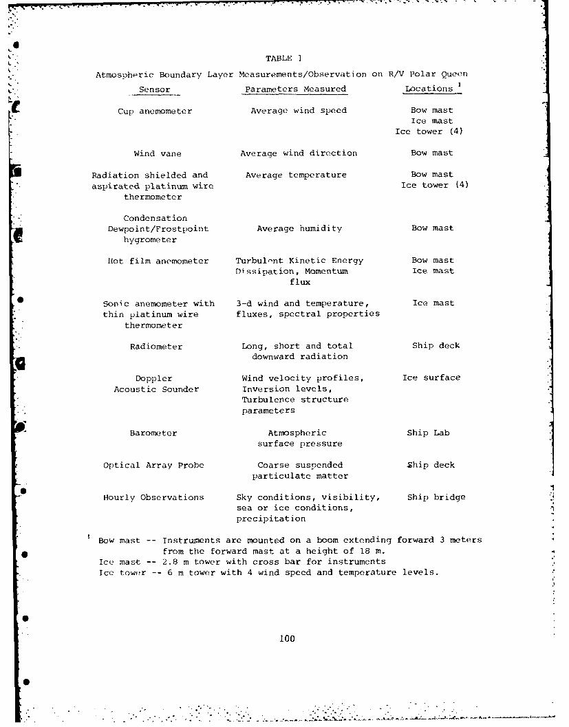
IT- To Pic _-F I I P.-.77 7

TABLE 1

Atmospheric Boundary Layer Measurements/Observation on R/V Polar Queen

Sensor Parameters Measured Locations 1

Cup anemometer Average wind speed Bow mast

Ice mast

Ice tower (4)

Wind vane Average wind direction Bow mast

Radiation shielded and Average temperature Bow mast

aspirated platinum wire Ice tower (4)

thermometer

Condensation

Dewpoint/Frostpoint Average humidity Bow mast

hygrometer

Hot film anemometer Turbulnt Kinetic Energy Bow mast

Dissipation, Momentum Ice mastflux

0 Sonic anemometer with 3-d wind and temperature, Ice mastthin platinum wire fluxes, spectral properties

thermometer

Radiometer Long, short and total Ship deckdownward radiation

Doppler Wind velocity profiles, Ice surfaceAcoustic Sounder Inversion levels,

Turbulence structureparameters

Barometer Atmospheric Ship Labsurface pressure

Optical Array Probe Coarse suspended Ship deckparticulate matter

Hourly Observations Sky conditions, visibility, Ship bridgesea or ice conditions,

precipitation

Bow mast -- Instruments are mounted on a boom extending forward 3 meters

from the forward mast at a height of 18 m.Ice mast -- 2.8 m tower with cross bar for instrumentsIce tower -- 6 m tower with 4 wind speed and temperature levels.

100

7 -a

II

METEOROLOGICAL ICE FLOE STATIONS OF HAMBURG UNIVERSITY

H.C.Hoeber

Meteorological Institute, Hamburg

Three automatic meteorological surface stations (HI, H2, H3 according to theMIZEX operations plan) were deployed on ice floes on 19, 21 and 23 June 1984, re-

spectively. Their position was monitored through the ARGOS system; the position

data set is included in the common data tape of all ARGOS platforms (ID code:

5430, 5431, 5432). "1

,4 Due to electronic malfunctioning which is believed to be caused by electrostatic

charging and discharging during the helicopter transport only stations HI and H2

delivered data comprising five minute averages of surface pressure, temperature,

wind speed and direction. The stations formed a triangle of 80 to 200 km sidelength

of which HI and H2 moved southward rather fast, while H3 deployed east of PO-

LARQUEEN remained almost stationary. The stations, therefore, were recovered on

1, 2 and 3 July 1984, respectively. A redeployment was scheduled but turned out to

be impossible after the necessary helicopter experienced a damage beyond repair

thus terminating this programme.

With the exception of wind speed at station Hi, the data - on first inspection - ap-

pears to be of reasonable quality. Small scale ice drift evaluation, however, will be

hampered due to the loss of the NOAA 8 satellite which caused a position data gap

each day between 5.30 and 12.30 GMT.

101

W -o -- - - - -2' 3- 4- E

H 3

301 H1 - 21 1 130,

8001 /1800

30' POASEN30'

I OL2~ R

u 790i. :102 I790W 30 2* 0 0 0 2 - Z ' 6

Fig. I -Hamburg automatic meteorological surface sta-tions on ice floes. Positions at first and last day of com-plete triangle deployment are shown, in addition to posi-tion of POLARSTERN.

102

IWind Stress and Micrometeorology From Kvitbjorn

*. R.J. Anderson and S.D. Smith, (BIO), R.E. Mickle, (AES)

The principal objective of this study was to obtain values of* wind stress and air drag coefficients for a variety of ice

types and weather conditions characteristic of the MIZEX area.

Another objective was to monitor the atmospheric boundary layerstructure and maintain detailed meteorological records for the

cruise.

Instrumentation: Sensors including a fast response propellorvane anemometer and microbead thermistor from BIO and cup and

* vane anemometer, relative humidity and air temperature from

AES were mounted on a bow mast. The BIO sensors are used formeasurements of wind spectra from which the wind stress can bedetermined by the dissipation method.

A three-axis sonic anemometer was deployed on the ice for moredirect eddy-correlation measurements of wind stress when it wasfeasible to work on the ice. Profiles of wind, temperature andhumidity through the atmospheric boundary layer were obtainedwith a tethersonde system winched from the ice and short andlong wave radiation were monitored with radiometers mountedover the bridge. A PRT-5 and thermistor probe were used tomeasure sea surface temperature.

Data Recording: The bow instruments were operational fromJuly 2-21 during which period 88 data runs of 15 to 45 minutes

duration were obtained by BIO and logged in digital format on

cassette tape. Qualitative observations of ice type and con-centration and some photos were taken especially for sonic

anemometer runs. Ice conditions varied from smooth to veryrough and from continuous unbroken ice to open water. The

sonic anemometer was operated during mini-drift phases only,with 30 runs obtained on July 4-7 and 15 runs on July 17-19.Comparison with the eddy correlation method will allow testingand calibration of the less direct dissipation measurements ofwind stress. Hopefully we can relate the roughness from the

4 laser profilometer line flown on July 6 to the wind stressmeasured by the sonic anemometer. Data from the first mini-drift period was the more productive since light winds (<5m/s)during the second period were less conductive to accurate deter-

*mination of the drag coefficient. Of the total BIO data set, 28runs had winds from 8-11 m/s and 57 runs had winds between 5-11

* m/s. -.

11

Routine meteorological data were logged as 5 min. averages forthe bow anemometer, air and sea temperatures, radiation, rela-tive humidity and air pressure for July 2-23. Standard logsheets of surface meteorological observations were completedevery 6 hrs. Satellite positions were logged every minute.Preliminary analysis of radiation data gives albedo as 5-7%.

The tethersonde system was deployed from the ice whenever the

ship was moored to a floe. The boundary layer profiles will be

used to help in the interpretation of wind spectra by thedissipation method and will also be used together with the4meteorological observations from other vessels to characterizeboundary layer conditions. Approximately 50 profiles to 100 mwere obtained.

104 104

II

WEATHER OBSERVATIONS - USNS LYNCH

R. A. Helvey

Upper-air and surface weather observations were made during MIZEX-84 on boardthe USNS Lynch by two personnel from the Pacific Missile Test Center (PMTC),while in the Greenland Sea from 8 to 24 June, 1984. Our primary goal was to

*" collect data for use in assessing the accuracy and representativeness ofmicrowave index of refraction profiles derived from several different types

of radiosondes, under polar maritime conditions.

Radiosondes employed were Beukers 1524 Microsondes, VIZ Research sondes, andVaisala RS80-15 sondes. The latter two measured only pressure, temperature

"- and humidity, but the Beukers additionally utilized Omega Navaid signals to

* obtain winds aloft. Termination altitudes varied from sounding to sounding,but typically at least 10 to 15 km were attained.

Because the Beukers system was not available soon enough before commencementof operations, familiarization trials and software modification to facilitateits use were carried out at sea. The first successful Beukers sounding tookplace on 16 June, with two to four releases per day thereafter up to themorning of 23 June. A total of 22 Beukers soundings were attempted during

this period, of which about 30% experienced serious problems in acquiring orarchiving data. In addition, from 13 to 21 June a total of seven jointVaisala-VIZ ascents were made, with the two different sondes strappedtogether side-by-side for comparison purposes. Performance of these twosonde types was generally excellent, judging from the raw data received.

Surface observations of pressure, wind, temperature, dewpoint, sea state and

sky conditions were made at intervals varying from hourly to six-hourly,depending on PMTC personnel workload and duty schedules. Bridge weatherobservations by the ship's crew were transcribed for two-hour intervals.One-minute average pressure, temperature and dewpoint measurements were alsocollected automatically and recorded digitally, although periods of data lossand calibration drift were apparent.

The radiosonde and surface digital data were recorded in essentially unreducedform on a variety of computers and media, and will require editing and other

processing before transfer to nine-track magnetic tape for inclusion in the

MIZEX data base.

105

.-. i1

WEATHER MAPS FROM VERVARSLINGA FOR NORD-NORGE, TROMSO

Erik Mollo-Christensen, NASA/GSFC, Code 671, Greenbelt, MD 20771

Weather maps were photographed at the Weather Forecasting Center for

Northern Norway (Vervarslinga for Nord-Norge) and Xerox copied for the

times listed.

I have saved slides of small scale maps (Fram Strait) at 127 for the

following Julian days:

169,170,172,173,174,175,176,177,178,179,180,181,182,183,184,185,186,187,

189,190,191,193,194,195,196,197,198.

4Additionally, I have saved the slides of small scale maps for the followingdays and times:

172: 06 Z, 09 Z, 12 Z, 15 Z,18 Z, 21 Z,

173: 00 Z, 03 Z, 09 Z, 12 Z, 15 Z, 18 Z, 21 Z

174: 00 Z, 03 Z, 06 Z, 09 Z, 12 Z, 15 Z, 18 Z, 21 Z

175: 12 Z

176: J0 Z, 03 Z, 06 Z, 09 Z, 12 Z, 15 Z

177: 00 Z, 03 Z, 06 Z, 09 Z, 12 Z, 15 Z, 18 Z, 21 Z

178: 00 Z, 03 Z, 06 Z179: 00 Z, 03 Z, 06 Z, 09 Z, 12 Z, 15 Z, 18 Z, 21 Z

180: 09 Z, 12 Z, 15 Z, 18 Z, 21 Z

181: 12 Z

182: 12 Z

183: 06 Z, 09 Z, 12 Z, 15 Z, 18 Z184: 06 Z, 09 Z, 12 Z, 15 Z, 18 Z, 21 Z185: 12 Z, 18 Z, 21 Z186: 00 Z, 03 Z, 06 Z, 09 Z, 12 Z, 15 Z, 18 Z, 21 Z

187: 00 Z, 03 Z, 12 Z188: 00 Z, 09 Z, 12 Z, 15 Z, 18 Z, 21 Z189: 00 Z, 06 Z, 09 Z, 12 Z, 15 Z, 18 Z

190: 00 Z, 06 Z, 09 Z, 12 Z, 15 Z, 18 Z

191: 00 Z, 03 Z, 06 Z, 09 Z, 12 Z, 15 Z, 18 Z, 21Z

192: 03 Z, 06 Z, 09 Z, 12 Z, 15 Z, 18 Z, 21 Z

. 193: 00 Z, 03 Z, 06 Z, 09 Z, 12 Z194: 12 Z

195: 12 Z, 21 Z196: 12 Z

The following maps are also in the form of Xerox copies, including the Fram

Strait and East Greenland, with a strip of the coast of Norway showing:

106

0.

169: 12 Z, 170: 12 Z 172: 12 Z, 173: 12 Z 174: 12 Z 175: 12 Z 176: 12 Z

177: 12 Z 178: 12 Z 179: 12 Z 180: 12 Z 181: 12 Z 182: 12 Z183: 06 Z, 09 Z, 12 Z, 15 Z, 18 Z, 21 Z184: 00 Z, 03 Z, 06 Z, 09 Z, 12 Z, 15 Z, 18 Z, 21 Z185: 00 Z, 03 Z, 06 Z, 09 Z, 12 Z, 15 Z, 18 Z, 21 Z186: 00 Z, 03 Z, 06 Z, 12 Z, 15 Z, 18 Z, 21 Z187: 00 Z, 03 Z, 06 Z, 09 Z, 12 Z, 15 Z, 18 Z, 21 Z188: 00 Z, 03 Z, 06 Z, 09 Z, 12 Z, 15 Z, 18 Z, 21 Z

189: 00 Z, 03 Z, 12 Z190: 12 Z 191: 12 Z 192: 12 Z 193: 12 Z 194: 12 Z 195: 12 Z 196: 12 Z197: 12 Z 198: 12 Z

Weather maps for every three hours are archived at Vervarslinga for Nord-Norge in Tromso, I have copied the above maps for the convenience of MIZEXproject participants, and because they are of direct interest in my own

research. The attached figure shows a copy of a slide showing the weathermap on June 24, when there was a low pressure in fram Strait during the

CV-990 overflight.

Additionally, I have copies of the ship reports, for the period June 15

through July 11.

The digitized weather maps still need some glitch removal processing andwill take some time.

107

0

• '" ° , % -. " , . .

p...

p.

p.°

REMOTE SENSING

109

-- 7

ERIM/CCRS CV-580 SAR DATA COLLECTION AND ERIM SURFACE

OBSERVATIONS DURING MIZEX 84

R. Shuchman, C. Livingstone, B. Burns, R. Larson

During the period 29 June-10 July, the CV-580 conducted 7 flights over theMIZEX experimental area in the Fram Strait and three additional missions overSvalbard and the Norwegian Sea. Synthetic aperture radar (SAR) imagery wascollected in all missions, scatterometer data on one flight, and aerial pho-tography as weather permitted. In addition to the aircraft activities, ERIMpersonnel also carried out surface truthing from the POLARSTERN, obtainingprimarily dielectric constant and snow wetness measurements of the snowcover. Both aircraft and surface efforts are summarized here.

The seven CV-580 missions over the experimental area each produced mosaicsof X-band (3.2 cm) and L-band (23.5 cm) SAR imagery. It had been plannedthat C-band (5.7 cm) imagery would also be collected, but due to breakageduring shipping, the C-band SAR could not be used. Mosaics of the area(approximate) 800 to 81ON and O to 40E were obtained on 29 June and 6 July,mosaics of the area 780 to 790N and 40W to 00 on 5, 7, and 9 July; and thearea 78030 ' to 80°N and 20W to 20E was imaged on 30 June. Three lines of

* dual polarization, dual frequency SAR imagery and one line of scatterometerdata were obtained on the night of 9/10 July in the area of the POLARQUEEN.

Based on the real-time imagery and the optical data processed to date, theSAR imagery show very clearly the changes in floe surface conditions as thesummer melt progressed and the dynamics at the ice edge. The mosaic obtained

. 5 July portrays the eddy structure at the edge especially well.

The objective of the surface program was to obtain measurements of the snowcover parameters critical to interpretation of remote sensing microwave data.Dielectric constant and snow wetness measurements were carried out with em-phasis on coordination with scatterometer measurements made from helicopterand ship, and with aircraft SAR, SLAR, or PMI data collection.

During the period 18 June through 14 July, nineteen sites were visited wheredielectric constant measurements with the 100 MHz Q-meter and the L-band coaxsystem were taken at various depths in the snow cover. For most sites, snowsamples were taken back to the ship and free water fraction measured in the

*cold room under controlled conditions. (Equipment for measuring the freewater fraction of snow was supplied by CRREL.) At two sites, snow wetnesswas measured on the floe, but due to the lengthiness of the measurement andthe shortness of the stations, this was not continued. Auxiliary data col-lected at each site included snow depth, crystal size, snow temperature, andsnow density. Nine of the site measurements were coordinated with shipscat

* measurements made by U of Kansas, five with U of Kansas heloscat flights,two with aircraft PMI overflights, and seven with aircraft SAR or SLARoverflights.

Conditions found during this period ranged from very dry, cold snow coverwith a crust to melting conditions. For these two extremes, free water

110S]

fraction (by volume) ranged from approximately 0% to 7.3%, dielectric con-stant (at the surface) from 1.45 to 3.2, and loss tangent from 0.007 to 0.07.Additional measurements of dielectric constant at X-band were made in thecold room on both first-year and multiyear cores obtained by the CRREL group.

In addition to surface measurements, an incident power receiver was placedon the deck above the bridge to record the antenna pattern of the aircraftSAR as it passed over. Incident power from the CV-580 SAR was recorded onboth 5 July and 9 July overflights. During the 9 July overflight, an activecalibration device and corner reflectors were placed on floes for both iden-tification and calibration purposes.

[I

II °II

4

REPORT ON FRENCH B-17 OPERATIONS IN MIZEX-84

W. Campbell, N. Lannelonge and D. Vaillant

T1ring the period 28 June through 19 July 1984, the B-17 of the National-fecraphic Institute of France (IGN) performed five mesoscale radar mosaic

m-rpping missions in MIZEX-84. The aircraft was equipped with the Varan S(1'homson-CSF/CST/IGN) X-band digital SLAR. The aircraft also was equippedwith the same Litton inertial navigation system as that used on the Concorde,therefore very accurate navigation was possible during the complex maneuversrequired during each mapping mission.

All five B-iT radar mapping missions were successful. Each took place underadverse weather conditions, and the flights were all timed so that theradar mosaic nmpjing occurred at approximately noon GMT on the day selected.Because the B-17 is not a fast aircraft (normal cruising speed is 140 nm/hour)and the distances were great, the duration of each flight was long; theshortest flight was eight hours and the longest was thirteen hours.

As fate would have it, the period of operation of the B-17 was also a periodof strong ice and ocean dynamics in the MIZEX area. Indeed, conditionswere changing so rapidly that the complex flight plan for each B-17 missionwas changed after take-off. An important advantage of the slow speed ofthe B-17 is that some time is available during the approach to the targetarea in which to change plans, an option usually not possible in fasteraircraft. Of course, high-quality navigation and flying is essential evenin a slow aircraft, and the success of the B-17 flights was due to theextremely high-quality performance of the IGN flight crew.

After each flight a cartoon of the radar mosaic data was made as quicklyas possible and transmitted to the POLARSTERN to aid in the executionof the experiment. These data proved to be very useful to the scientistsin the field. During the last three flights, when the surface was completelycloud covered and much fog was present, the B-17 radar data was used in

6 a real-time mode when data from facsimile charts were transmitted by radioto the ships. In short, every effort was made to get useful B-17 radardata to the field scientists as rapidly as possible.

* "The data selected for each flight were determined amid an array of variablefactors - joint missions with other remote sensing aircraft, surface condi-tions, weather, logistical problems, etc. The flights occirred on thefollowing days: 30 June, 6 July, 11 July, 14 July and 16 July 1984. The

* first flight was flown out of Tromso with a return to Tromso. This modeof operation proved to be excessively consumming of aircraft flight hours,so the decision was made to switch operations to Longyearbyen. Thus, theflight of 6 July originated in Tromso and ended in Longyearbyen, the flights

* of 11 and 14 July originated and ended in Longyearbyen, and the flightof 16 July originated in Longyearbyen and ended in Tromso.

The five radar mosaics obtained by the B-17 cover oar e sea ice and oceansareas, the average area being approximately 1.3xlO km5. The shape andsize of each radar mosaic varies and was determined in the trade-off between

112

. i1.maximum coverage and available flight time. The coordinates of the corners

of each mosaic flight are:

30 June: (1) 79°48'N, 04°40'E

(2) 780 55'N, 04°40'E

(3) 78055'N, 01O00 'W

(4) 79o48'N, 010 00'W

6 July: (1) 79053'N, 030 15'E(2) 790 00'N, 030 15'E

(3) 790 00'N, 020 00'W(4) 790 53'N, 020 00'W

11 July: (1) 78 0 40'N, 010 00'E

(2) 77 057'N, 020 05'W

(3) 78041'N, 050 40'W

(4) 79o16'N, 02030'W

plus two overlapping bands covering a width of %16 nm

extending from the center of the NW side of this box to:

(5) 79045%N o6037'W(6) 79034'N, 06040'W

plus one band covering a width of %8 nm extendingfrom (5) to (6).

14 July: (1) 790 30'N, 000 30'W(2) 79000'N, 020 30'E

(3) 78°06'N, OI°40'W(4) 78037N, 04o30'W

16 July: same as 14 July.

The immediate task is to process this vast amount of high-quality digital

SLAR data. This is a formidable task! A study recently performed at CNES

(French Space Agency) Toulouse showed that to process a 20 km x 20 km area

of the data on the largest computer at CNES will take six days. To process

all the B-17 MIZEX-84 data would take approximately three years. Since

there is no way that CNES can devote their largest computer to us for years,

we must explore other means for processing. This problem will be discussed

at a French MIZEX Remote Sensing meeting at CNES-Paris on 24 September 1984.

4

113

• - - ..~% . .. .- - - - . . - . . , i J . . , .'-.. . :.- i

- .~- !

NRL RP-3A MIZEX 84 EXPERIMENT REPORT

J. P. Hollinger M. R. KellerNaval Research Laboratory Bendix Field Engineering uurp.

The Naval Research Laboratory conducted airborne microwave radiometric imagingmeasurements at 90 GHz over the marginal ice zone in the Greenland Sea usingthe NRL RP-3A aircraft from 26 June to 9 July 1984. In addition, microwaveradiometers at 19, 22, and 31 GHz were used to obtain profile measurements atnadir. Details of the radiometers are given in Table 1. Environmentalsensors provided pressure, air temperature, dew point temperature, and liquidwater content. The aircraft inertial navigation system (INS) provides windspeed and direction at the aircraft altitude as well as pitch, roll, trackangle, heading, latitude, and longitude. A PRT-5 infrared thermometer wasused to obtain surface temperature, a 70 mm Hasselblad motorized frame camera4 was used for aerial photography, and a trained ice observer participated inthe flights to define ice type and coverage from the aircraft when visibilitypermitted. Two sets of flights were made. One set consisted of three flightsat 7.56 km altitude to map a 117 by 139 km region containing the marginal icezone at 90 GHz. The other set consisted of a flight at 1.8 km altitude tomap a 52 by 123 km region of the ice pack at night, and low altitude (0.9-1.8km) flights to obtain high resolution data at all the microwave frequencies.Emphasis was placed upon coordinating with ground truth surface teams toassure exact correspondence between surface truth measurements and the airbornemicrowave data.

Flight I was flown on 26 June 1984 at two altitudes (Figure 1). Twelveparallel tracks were flown at 7.6 km to collect the data for the first 90 GHzhigh altitude map. Three legs were flown at 0.9 km to obtain 19, 22, and 31GHz profile measurements at nadir in the area of POLARQUEEN. Flight 2, flownon the night of 28 June, consisted of nine parallel tracks, which were flownat 1.8 km (Figure 2). This 90 GHz high resolution map will be used to examinethe microwave properties of summer ice during night time freezing conditions.A tenth track, flown at 1.2 km, produced 90 GHz imagery from the interior ofthe pack through the loose ice to open water. The 90 GHz image data for thesecond high altitude ice map were collected during flight 3 (Figure 3), on 2July 1984, which consisted of twelve parallel tracks at 7.6 km altitude. Twoparallel tracks to and from the north pole, were flown during flight 4 on 4July 1984 (Figure 4), to obtain 90 GHz imagery of the ice pack to the pole.During flight 5, on 6 July, 90 GHz imagery of the area around POLARQUEEN andPOLARSTERN was generated. Six tracks were flown over the POLARQUEEN atvarious altitudes (Figure 5). Tracks 1 and 2 were flown at 7.6 km, track 3and 4 at 3.7 km, track 5 at 1.8 km, and track 6 at 0.9 km. The last fourtracks of the flight were flown at 0.9 km over POLARSTERN. The sixth andfinal flight was on 9 July. Twelve parallel tracks were flown at 7.6 km(Figure 6) to produce the data for the third 90 GHz high altitude map.

Excellent 90 GHz data were collected during the six flights, but were occa-

sionally marred by radio frequency interference (RFI). This problem was

especially severe throughout the first flight on 26 June, when RFI was presentnearly all the time. Profile data were collected at 19, 22, and 31 GHz. The

* 22/31 GHz radiometer produced consistently good results on all flights. OnJune 26 (flight 1) and July 9 (flight 6), the 19 GHz radiometer malfunctioned,

114

causing it to either fail or produce inconsistent calibrations. For themajority of the rest of the flights, the 19 GHz radiometer was stable andyielded accurate data. Since the marginal ice zone was cloud-covered duringmost of the mission, 35 mm and 70 mm photography was only taken during breaksin the clouds. Thus, on 26 June (flight 1), 2 July (flight 3), 6 July (flight5), and 9 July (flight 6), photographs were taken intermittently. On 28 June(flight 2), and 4 July (flight 4); however, because of clearer conditions,more continuous photographic coverage exists.

Data reduction for MIZEX '84 will commence upon the complete installation ofa new computer. The high altitude ice maps and night mosaic should be reducedby spring 1985, and the ship passes and polar flights by summer 1985.

1

0

*1I7

115

. , .. .. . 4 . . . . . . - : . , " ,.•- .. ..- . -. -. °. . -- , ° °

TABLE I

NRL AIRBORNE RADIOMETERS

Center Frequency Wavelength IF Frequency System Sample MS Noise Ilalf-Power

GHz mmin Noise,K 1 Rate er Sample Beamwidth

Imaging Radiometer .

90.0 3.3 to 2.2GHz & 1,700 2.4 KHz! 1.4 1.012.9 to 5.2GHz

Profiling Radiometers

19.3 H & V 15.5 1 30 to 300MHz 1,000 10 Hz 0.5 8.0

22.2 V 13.5 (5 to 500 MHz 1,000 10 Hz 0.4 8.0

31.0 H 9.7 5 to 500 MHz 1,000 10 Hz 0.4 j 8.0

82 6 26 84 82 6 28-29 84

81 81

5 - 4

-~~~ ;{i{i1 44

NOTE1 LE4 1374 5AERDOEE

79 R

8o ,,,, ~98' 5 z° 7o 6

00

NOTE: LEGS 13, 14, 15 ARE RADIOMETER !

79 - RUNS OVER POLARQUEEN 79

I l I I I I I I 2 I I ! I I I

S0 1 2 3456 7 8 1 0 1 23 4 5 6 7 8 9 10 11 12WEST WEST

LONGITUDE (1) EAST TUDE I') L ONGTUDE ( ) EAST LONGITUDE I')

Figure 1. Flight 1 track pattern Figure 2. Flight 2 track pattern

116

IL

4

82 7'2/84 817/4/84FROMNORTH POLE TO NORTH POLE

81 80

S 12 11 10 9 8 7 9

z c

a0

L 12 10 1L L 4 7 10 11 12 7 32 -2 3 4 5 7 8 90

WEST EAST LONGITUDE Mo WESTLONGITUDE ()LONGITUDE M° EAST LONGITUDE )

I--

Figure 3. Flight 3 track pattern Figure 4. Flight 4 track pattern .81 7/6/84 82 7/9/84

80 -81-

zz

79 8 _

II

18 79-

.L , I I I I I I I I I I t I I I I I I I I I I I | I I

3 2 1 0 1 2 3 4 5 6 7 8 9 10 21 0 1 2 3 4 5 6 7 8 9 10 11 12WEST WEST EAST LONGITUDE (°LONGITUDE I*) EAST LONGITUDE T LONGITUDE MFigure 5. Flight 5 track pattern Figure 6. Flight 6 track pattern

117'

• ]-

. . -, • -• . . •0

.2 2. .2•2

IF

NASA/CV-990 ACI'IVITIE.S DURING MIZFX' ,t

Per (;loerszn

General -Of the thirteen test, transit, ald local flights nde by tile NASACV-990 during this campaign, nine of them had data pertinent to MIZEX'84 andare outlined below. %lien mosaic patterns were floii, they were from analtitude of ca. 5 tim with legs 10 irn apart.

Day 160 - 6/8 - Ames/Thule - Transects - Some sea ice data were obtained overHudson Bay, Foxe Basin, and part of Baifin Bay. Excellent conditions for

useful albedo measurements were obtained -- both high aid low level.

Day 161 - 6/9 - Thule/Evenes - Six-leg North/South Mosaic - Center near 81 N,6' 10'E - Cloudy - Polarqueen was estimted to lie between the two centerlegs, about 60 km frxn the southern edge. The real-time airborne ESIR imagesindicated that the ice was near or above the melt point over the entire MIZEXarea.

Day 164 - 6/12 - Evenes RT - Six-leg North/South Mosaic - Center near 81*N,80 1O'E - Mostly cloudy - Polarqueen was directly underneath us on thewestern ost leg of the mosaic pattern. The ER mosaic prepared on boardshowed that the ice was below freezing in the southern part of the MIZEX box,but at the melt point elsewhere.

Day 170 - 6/16 - Evenes RT - Long Four-leg North/South Mosaic - Center near810 45'N, 50 E - Partly cloudy - Freezing conditions were found in the MIZEXbox and near-melt conditions further north. This was coupled withobservations of scattered ice-clouds over MIZEX and heavy clouds north ofthere. Polarqueen was situated between the two westernmost legs. We were -'

startled to find the sea ice extending some 110 km south of the edge asobserved on the first leg; possibly we were observing part of an eddy. Thisinformation was radioed to the Polarqueen as we departed the area.

Day 174 - 6/20 - Evenes RT - Five-leg North/South Mosaic with 500' repeat ofcenter leg - Center near 800 36'N, 60 20'E - Cloudy - The center legs werecoincident with intensive surface meaurements and the NOAA P-3 transect. Theconditions were generally warm and cloudy over all of the MIZEX box,accompanied by the radiometric sigmatures typical of sea ice near the meltingpoint. In addition to providing an excellent visual evaluation of iceconditions along the low-level transect, we obtained albedo measurements ofthe solid pack, the ice margin, and the open sea with varying wave structure,albeit with a solid overcast. The low-level transect was extended to about790 30'N. The visual observations confirmed the presence of fresh snowfallover the entire area. Meltponds, although comprising less than 1% of the

* entire area, were observed to contain water.

Day 176 - 6/22 - Evenes RT - Six-leg North/South Mosaic - Center near 80°

40'N, 4'E - Cloudy - Both Polarqueen and Polarstern were within the pattern.The two easternmost legs were spaced 5 nm apart so that both the radiometersand the altimeter could repeat observations of the Day 174 low-level run.

* About 100 km south of the east/wst ice edge, an ice streamer, about 25 kIn in

118 4*

0 2" .. . • ',: ,;.: . .,.i " " ' " " " " " ' " ""

extent, was observed to mander mostly due east and then south. The MIZEXarea appeared rather compact, with relatively few open leads all less than Ikm wide in evidence. The pack signature was monotonously that of MJist seaice, so the floe structure was indistinguishable. The ice edge in the MIZEXbox was quite compact, but had an astonishingly regular sine-wave patternwith a wavelength of about 28 kIn. About 2-1/2 oscillations were observed.solitary thin ice band, ca. I km wide, was observed running east/west aboul30 kin south of the edge across the two easterunost legs.

Day 178 - 6/26 - Evenes RT - Six-leg North/South Mosaic - Centered near .;°

30'N, 2' 30'E - Partly cloudy - While there were some interesting (cold)multiyear ice features to the west, this was definitely the day for ice edgeobservations! The MIZEX ice edge was quite compact and following its recenteast/west sinusoidal undulations in the easternmost legs. As can be seen inFigure 1, a distinct change in orientation occurred near the middle of thepattern, running from southwest to northeast at a 45 degree slant across ourtracks, still compact, and still undulating sinusoidally. To the west, therewas clearly evidenced an eddy feature as delineated by the diffuse rings ofice shown on the airborne EMI image in Figure 1. Just south of that can be

* seen the so-called "dog's head" feature which gives the imipression of icefloes having been projected outwards by the edge of the eddy, at the rate ofat least 55 km in two days since these floes were not there during our priorflight two days earlier. The same feature is indicated in the R image forDay 178 (Figure 2), in which the ice edge is shown as a solid line, the iceedge four days later as dashed, and the rxsaic location as a box.

Day 180 - 6/30 - Evenes RT -Transects along Ice Edge - A rosette pattern wasflown over Nordaustlandet. The remaining tire was used to fly astraight-line transect between 800 20'N, 15*E to 800 20'N, 5W. We returnedon a parallel line 5 nm north of that to the 0 ° 30.8'E neridian and headedsouth to a latitude of 790 30'N, the predicted location of the northern edgeof the eddy. The east/west transect over the sea ice was clear, and affordedthe opportunity for some excellent photography of sea ice. The lack of cloudcover also resulted in below-freezing ice temperatures and the strongestmultiyear microwave signatures observed on this mission. We were not sofortunate in our attempts to obtain microwave imagery of the large eddy,since it had drifted southwards and outside of the preselected imager swath.It was easily observed visually, however, with about the swme eastward extentas before.

* Day 182 - 6/31 - Evenes RT - Five-leg East/West Mosaic - Centered at 79015'N, O°W - Clear - The two northernmost legs were extended to ca. 12°E inorder to overfly Polarstern. The "dogs's head" ice formation was still

* intact, although it had drifted about 30 km south and was more diffuse,indicative of loss through melting. Within the nosaic, the pack was quiteunconsolidated, with concentrations running 50% or less all the \ay to thePolarstern.

119

OOLON. DAY1 178

80N

0.

S - Figure 1-

120

* * 000000000000000000++8+8 / 6=.066**..**4.400000000000000000000+8+ /46442=4*4 1.6*..00000000000000000+0++/6 ... 4** 0/6/6)* 4.

* *000000000000000000+0++//6.4 == .8 +-81+ * .*.* 00000000000000000000808 . .64 *8+8 ..

* 00000000000000000+0+/044/24== ... 1-. **4..*0000000000000000000++0W 0 ..- /+00*00000000000000000000682 ..=224 +- 8 /

0000 *00000000000000000088/. 8.5f20000000*000000000000000000/4' _;

* 00000000*0000000000000000 _ 4-000000000000*000000000000008+ 40----0000000000000*00000000000000866 :-=++*/00000000 000000*000000000000086 /82'28000000000000000 *00000000008+42 88+00000 00000000000 *0000000+0888= - =. + :+t

000000000000000000 *00++ 88++ +800000000000000000000*00+0+ 4

o 0000000+00000++0++00+*+ 06662-u =4=46/6.4* *

0000000+0++++00++00+++ ++ .= *.4=8.8..==."4

0000000+0+8+00 ........... 0=4---------------- 22 =.400000+888+88+88 ....... 88+ 4 -- --

* 0088888888+.++.++.886 -- 2 - -- --0000 0 8 /88++8888+884 b - -00 0 8/ /+888888 1 .00 88 864664888888+8**86/ - -o / 6. /88888888/6. - --0 II 9.668668888*888Z///64= --

0 1/6.-=-=4..8/+884,=- ---

*++8 6* .4.*/88/4=*++ 4=4.4**6..6 t688/4. --

+ + .. **.. . .6 ,/6 Z0+0+.66... .' /6

+000* * 8 f .6.6/z 4i---~++000 *0 0 /6.666666%/4/4..4--8+00* 0 /~~ 6866668Z 4/ Z.4 --8+** 00* 0008088848///64// 44= --*** 0000 0000+8+8 8+1W1288--/+ 0000 0000+8+..8 8W/884+44/.48+00 0 00~0+ .. 888488888 /.=

0608 00 000000+....8+888++887/4=4++ 000 000000+++++888888+888//66.=2 -

6 +000 0000+.......8+888+8887Z64.L 8080 00000+......8888++88 /66..2 -

*6**(800 0 0000+......88+888888 /6- ---

Figure 2-i

121

PRELIMINARY MISSION REPORT

RUTHERFORD APPLETON LABORATORY OPERATIONS ON THE

NASA CV990 FLIGHTS DURING MIZEX 84

R.J.Powell and A.R.Birks, Rutherford Appleton Laboratory

The Rutherford Appleton Laboratory (RAL) has been responsible for the con-

struction of a microwave altimeter/scatterometer and its deployment in a

NASA Convair 990 flying Laboratory during the period 7-30th June 84. This

work has been undertaken in support of the ESA ERS-I radar altimeer pro-

gramme, the Marginal Ice Zone Experiment (MIZEX) and collaborative research

programmes within RAL, University College London, Mullard Space Science

Laboratorty, Scott Polar Research Laboratory and Oxford University.

*The activity has been supported largely by funds from UK Science and

Engineering Research Council, who support this team of scientists at RAL

and ESA who have provided about half of the flight costs and a study con-

tract under which the resulting data will be analysed.

RADAR ALTIMETER - PRODUCT DEVELOPMENT OVER THE MIZ

It is clear from the flight tracks that a great deal of data was collected

* in the MIZ. Some points of particular interest are: -

o A line running into the ice from the ship Polarstern wasvery thoroughly with nadir scatterometric measurements at

13 GHz and photography from a helicopter plus surface

sampling. This line was oveilown by the altimeter twice

at 33,000 ft and once for albido measurement at 500 ft.

o Data for ocean wave spectra determination was collectedwhile passing from the ocean into the ice on several occa-

sions.

o Similarly H1/3 data was collected.

o SAR 580 images were collected on 30th June coincident with

RAL H1/3 and wave spectra data.

MEASUREMENT OF a AND SWH OVER THE OCEAN

Suitable data was collected over the MIZ and on the ferry legs to and fro.However, ground truth is generally only available in the MIZ where ship,

SLAR and SAR has been taken with close coincidence.

There is probably no coincident RA, and laser profiler data over the sea so

that a wave-bias study will not be possible.

Some information on the variation of a with altitude may be obtainable from

the flights at 500 and 30,000 ft and Relicopter data measured in the same

region.

122

. h. . .

Participation in the NOAA P-3 Aircraft in the 1984 Summer MIZEX

L. S. Fedor-.- NOAA, Wave Propagation Laboratory

The principal investigators participating in the NOAA portion of the 1984summer MIZEX are L. S. Fedor, J. Overland, D. Ross, and M. A. Shapiro ofNOAA and C. T. Swift of the University of Massachusetts. The instrumentationon board the NOAA aircraft included: Ka band SLAR; LASER; C-band step-frequency radimeter; gust probe; up, down, and side radiometers coveringfrcum 0.3 pn to 14 pm; cameras; amega drop windsondes; airborne expendablethermographs; and flight-level data. Because of space limitations, theLASER and SFWR could not be flown at the saue tine. On two of the missionsa total of 128 SUS charges were dropped in support of the _ astics research.A total of six research missions were flown, each of approximately 9 1/2

.* hours duration. The SFM was on Missions 4 and 5. The LASER was on for theother missions. An ice observer, AGI Carl Newton fran the Navy/NOAAPolar Ice Center was on board for all missions.

MISSION #1, 20 June 1984 - BOUNDARY LAYER: Winds in the operating areawere generally northerly 6-8 m/s, The wind drag stacks were oriented onthe KVITBJORN with the cross-wind legs towards the West. A total of 2 1/2stacks were ccupleted with the gust probe, SLAR, and LASER all obtaining

* good data. Only one AXBT successfully transmitted data for calibration ofthe downward looking PRT-5 radicmeter. There was 5/10 ice coverage inoperation area nearly all first year ice.

MISSION #2, 22 June 1984 - ACOUSTICS #1: Two long legs oriented North-Southand East-West rre oentsred over the KVITBJORN. There were too short legsoriented at 45 and 315 from the KVITBJCRN. A total of 64 SUS chargeswere dropped (two became inbedded in the ice). Only 8 of 16 AXBT's trans-mitted data. At the ends of the North-West and North-South leg, we encount-ered 9/10 and 6/10 respectively of multiyear ice. By flying a dog leg wehave the opportunity for good directional measurements of multiyear iceby the LASER. A North-South run at 5000 feet was made to give a goodsurvey of the area from the SLAR.

MISSION #3, 24 June 1984 - ACOUSTICS #2: The flight pattern for thismission was a repeat of Mission #2. There was a strong southerly wind of20 kts onto the ice dropping to 2 kts at the edge of the pack. We had aweight problem with the SUS charges on board and had to leave the gust

* probe sensors and the engineer in BODO. Again 64 SUS charges were dropped.Of 16 AXBT's dropped, ten transmitted good data. In the open water therewas mixed swell conditions-longer swell from the South and shorter swellfrcm the East with sane white caps on the surface. Inside the MIZ, wherethe wind had dropped off, the LASER would lose track going fran ice floeto open water which was very smooth. Open water surface temperatures

6 were 0 30C. Rain showers and turbulence were encountered in the easternand southern parts of the flight pattern.

MISSION #4, 30 June 1984 - REMTE SENSING SURVEY: A square-wave patternwas flown covering an area 100 nm on a side. The pattern covered an areafrn outside the MIZ to well into the pack. The northwest corner of the

I

123

I-

pattern was over 9/10 MY ice. At least three MIZ eddies were overflown withthe largest at the southeast corner. Some swell was observed entering thearea frcm the East, otherwise the water surface was very smooth. The SFMRreplaced the LASER on this mission. The survey was flown at 5000 feetexcept for a 500 foot run diagonally across the pattern for low level SFMRand SLAR data comparison. We dropped four AXBT's in the largest eddy on thelast run.

MISSION #5, 4 July 1984 - ICE EDGE SURVEY: The Ice Edge was flown fromnortheast of SPITZBERGEN to 30W. The principal instruments were the SFMR,SLAR, and PRT-5. We dropped 15 AXBT's both inside the pack through and out-side the MIZ. Visual observations east of the MIZEX operations area weremarginal because of heavy low-level clouds. Pack ice was 9/10 MY. A legwas flown in the MIZEX operations area for data coparisons with the U.S.Navy and NORWEGIAN P-3's. West of the MIZEX operations area we encounteredmostly FY ice with open water surface temperatures of 4.0 to 4.5°C. Three

SAXBT's were dropped in the Gulf Stream in returning to BODO.

MISSION #6, 6 July 1984 - METEOROLOGY FLIGHT: A low pressure system movedfrom NORWAY to SPITZBERGEN on the 5th, 6th, and 7th of July. Strongesteffects in the MIZEX operations area occurred late on the 6th. An ODWsurvey was made from BEAR ISLAND to the MIZEX area with five ODW's. We willneed the 12Z soundings fran BEAR ISLAND and weather ship AMI. There werestrong northerly winds in the operations area but attempts to fly windstress stacks were foiled by the low cloud base. Nevertheless, we wereable to see the surface at nadir and 90% of the LASER data is good. Numerousupwind and downwind legs were flown over the KVITBJORN and POLAR QUEEN. Atleast one downwind leg was directly over the KVITBJORN. Upon leaving thearea, one ODW was dropped at 78.22uN, 2.60E. A total of five AXBT's weredropped in the Gulf Stream on returning to BODO.

1

~124

I

SLAR AND LASER OBSERVATIONS OF SEA ICE DURING MIZEX '84

Duncan B. Ross and John Tcachay

NOAA, Miami, FL

Real aperture radar imagery at 35 GHz and laser profilcmetery wereobtained of sea ice in the marginal ice zone from a National Oceanic andAtmospheric Administration RP3C turboprop aircraft during June and July of1984. SLARI) data were obtained on 20, 22, 24 and 30 June, and 4 and 6 July.Figure 1 presents an example of the characteristics of the MIZ on 20 June inthe vicinity of 80.3N and 6.45E during off ice winds of 5-7 rps. The iceconsists of small pancake floes fairly well dispersed due to the local windconditions. Figures 2, 3, and 4 show the MIZ at the same region on 22 Junewith winds of 1-2 rps from about 40 degrees. The small floes have quicklyadapted to the pattern of the surface current regime which displaysconsiderable complexity. Nearby, at 80.45 and 3.27E Fig. 5 shows the moresolid pack to be heavily rotted, with many small floes broken off the largermultiyear floes. Fig. 6 presents evidence of another well developed eddystructure at 78.9N and 2.44E. The surface wind of 4 ups was blowingessentially off ice (from 340 degrees).

Laser profilcmetry data were obtained on 20, 22, and 24 June, and 6July. The data were generally of high quality and included the laseraltitude, phase shift, and signal amplitude signals. The data were recordeddigitally at a frequency of 80 samples per second.

High quality imagery and profilcmetry have been obtained over the MIZwhich will allow objective determination of ice concentration and roughness.The imagery were obtained at various altitudes which may allow develcpmentof algorithms to extract ice age information. Ocean surface currentpatterns were imaged through their ice signature. Wave conditions ere

* generally too benign to image, but some imagery of waves within the MIZboundary were obtained.

S

a

125

I

...-. --------. . -

e

... ....... , ,, . m , 1 I.~j .aL

;V~ 4

NR,~

0

1 26

(FIGURE 4. 212 JLurseq 1984. 60.23N- 3.47E. AltItUde 145M. U10'=1 -3rflos

46

FIGURE S. 30 June, 1984. 76.9N; e.4E. Altitude 1500M. U.10=4-5rnos

127

I

ACTIVE MICROWAVE MEASUREMENTS OF SEA ICEIN THE MARGINAL ICE ZONE

R.G. Onstott and R.K. MooreRemote Sensing Laboratory

University of Kansas Center for Research, Inc.Lawrence, Kansas 66045-2969

The primary objective of the near-surface radar backscattermeasurement program was to describe the scattering coefficients Qf seaice and ocean in the marginal ice zone (MIZ) in order to understandtheir influence on the microwave properties of ice and ocean in theregion. These and physical property measurements were coordinated withthe active and passive microwave aircraft measurement program. Radarbackscatter data were acquired, using the University of Kansas heli-copter-borne scatterometer (a calibrated radar) at 5.2, 9.6, 13.6 and16.6 GHz, at multiple angles from 0 to 700, with VV, HH and HVtransmit-receive antenna polarizations. In addition, a calibrated radaroperating at 1.5 GHz and HH-polarization was installed on the icebreaker"Polarstern". Its viewing angles ranged from 170 to 500.

Sites investigated included small-to-vast first-year, thick first-year and multiyear ice floes which were visually representative of ice

* types in the MIZ and pack ice region. Ice thicknesses ranged from 30 towell over 300 cm. Snowpack was heavy, with depths up to 60 cm on manymultiyear ice floes. During the experiment period the snowpack and icesheets underwent a transition from early-summer to summer-melt condi-tions.

Auxiliary measurements, to be used in the study of the radaraltimeter response of sea ice and ocean, were made with a vertical lookangle at 5.2 and 13.6 GHz. Additional measurements, transects, weremade to study the relationship between the radar response and oceanphenomena such as fronts at the leading ice edge and eddies, as well asthe relation between the radar response and ice concentration.

General ice condition descriptions, oblique photography, anddetailed descriptions of snowpack construction were made in support ofnear-surface and aircraft observations.

0

0

128

- . - ° -.- ..- .... • - . . ,... . . .- -- ..- -. .- -- - - . .

FICE MICROWAVE REMOTE SENSING EVALUATION PROGRAM

Prime Investigator: C.Schgounn (Irance)

Three active sensors have been involved in the remote sensing program. The

overall purpose was to make measurements at different scales in time and

space to study radar signatures of various ice-type during summer months

at different frequencies, polarizations, angle of incidence.

I RAMSES PROGRAM

Instrument manager: E. CHAPUIS.

The ground based frequency modulated radar RAMSES II on Polarstern will

provide in situ measurements for the whole period on different ice-conditions. Mesurements have been done at 5.3, 9.4, 13.6, 16 GHz for like

polarizations during stations in the ice.During each station one to six

curies from 0 to 60 degrees of incidence have been obtained . Data are

summarized in table 1 - pictures of surface during stations are available.

*O II ERASME PROGRAM

Instrument manager: E. CHAPUIS

Measurements with the frequency modulated radar ERASME working at 5.35 GHz

-. on helicopter AS 355 have been done along tracks approximately 200 km long.

The purpose is to study ice/water transitions, ice/water concentration and

ice characteristics. Each track corresponds to a given incidence and

polarization. Video recordings have been correlated with flights.

Data are summarized in table 2.

120I

01

*I

129

S1

TABLE 1

Date Lat. Long. 5.3 9.4 13.6 16

HH VV HH VV HH VV HH VV

169 79.17N 3.29 W x x171 80.80N 3.13 E x x x x171 80.80N 3.04 E x x x x x x173 80.32N 6.52 E x x x174 80.14N 2.57 E x x x x175 80.12N 2.57 E x x x x175 80.11N 2.52 E x x

175 80.80N 2.17 E x177 80.13N 2.03 E x177 80.13N 2.03 E x177 80.10N 1.59 E x x178 80.20N 1.00 E x x178 80.20N 2.13 E x x x179 80.22N 1.26 W x x x x

180 80.39N 5.36 W x x x x

180 80.35N 5.24 W x x180 80.20N 3.22 W x x182 79.23N 10.41 W x x x

183 79.25N 4.17 W x x x183 79.2 N 2.48 W x x x185 80.24N 1.17E x x x

186 80.19N 1.29 E x x x

187 78.25N 00.28 E 1 x x

188 78.25N 05.04W x x x189 78.41N 2.19W x x x x

190 78.56N 1.25 W x x x x

191 79.36N 6.38 W x x x x192 79.31N 6.26 W x x x x x

193 79.41N 6.41W x x x x x x194 79.47N 5.,2 W x x x x

195 79.48N 5.28 W x x x x x

196 79.47N 3.53 W x x

6 197 79.36N 1.22 W x x x x x

198 79.OON 00.39 E x x x x x198 79.12N 00.08 W x x x x

13

130

0Date 180 Incidence 27 Pol VV

Alt. 1100 f.

1 track Lat. 82.19 N Long. 04.25W to 03.00 E

2 track Lat. 80.30 N Long. 03.00E to 03.30 W

Date 180 Incidence 100 Pol VV Alt. 1100 f.

* 1 track Lat. 80.20 N Long. 04.25 W to 03.10 E

2 track Lat. 80.30 N Long. 03.04 E to 04.25 W

L0

Date 182 Incidence 5° Pol VV Alt. 1100 f.

1 track Lat. 79.15 N Long. 08.20 W to 02.00 E

2 track Lat. 79.15 N Long. 02.00 E to 08.20 W

Date 182 Incidence 400 Pol VV Alt. 1100 f.

1 track Lat. 79.15 N Long. 10.28 W to 00.00

2 track Lat. 79.15 N Long. 00.00 to 10.28 W

0Date 188 Incidence 25 Pol HH Alt. 320 f.

1 track Lat. 78.24 N Long. 05.27 W to 00.50 W

2 track Lat. 78.24 N Long. 00.50 W to 05.27 W

TABLE 2

131

UNIVERSITY OF WASHINGTON MICROWAVE EMISSION PROGRAM

Thomas C. Grenfell

Surface based observations of radiometric brightness temperatures over seaice were carried out from 8 June through 16 July from M.V.Polarqueen.Measurements were made at frequencies of 6.7, 10, 18.7, 37, and 90 GHz inboth vertical and horizontal polarization as a function of position along

ghorizontal traverses of 50 to 200 meters in length and as a function ofnadir angle at indivdual sites. Twenty three different sites were in-vestigated over the course of the experiment. Unfortunately, the Gunndiode in the 37 GHz instrument burned out during the first week, and wewere not able to repair it on site. Thus 37 GHz data could not be obtainedafter that time.

Measurements were made over the range of surface types encountered. Theseincluded both bare and snow covered ice from cold conditions (-7 to -100 C)

through to melting summer ice. Multiyear, thick first-year and frozenlead surfaces (identified last year as thin first-year ice) were studied.Observing times were chosen specifically to coincide with overflights by

* the NASA CV990, the NRL P3, and the CCRS CV580 aircraft. This effort inturn was carried out on even days of the month in order to coincide withscheduled SMMR imagery.

In conjunction with the radiometric observations, an extensive program ofsurface characterization was carried out. Along each of the radiometertraverses, detailed studies were made of surface topography, spatial var-iations in snow depth, the occurrence of ice layers and lenses in the snowpack, and ponding of meltwater. These were compared with the correspond-ing radiometric records. At selected locations, surface characteristicswere determined from core samples. For cold ice cases, these measurementsincluded temperature, salinity, and density profiles in the snow and thetop 30 cm of the ice together with the geometry and mean size of the snowgrains. When the ice entered the transition to melting stage, free water

content measurements in the snow and loose upper layers of the ice wereincluded in the program. The crystal geometry and density of the loosegranular layers were also obtained.

At the snow/ice interface, salinities near zero were found even during thecold weather suggesting that prior melting events had taken place in the

marginal ice zone. This conjecture was supported by the presence on the

first drift floe of extensive snow free areas with a smooth surface andrecrystallized structure in the upper few centimeters of the ice. As a

result, the ice tended to show a multiyear-like signature (brightness

* temperature decreasing at higher frequencies) over certain areas of the

first-year ice.

Early in the experiment, pressure ridges and compacted snow drifts showeda decreased brightness temperature most notably at the higher frequencies.Later in the season, these areas often responded faster than the surround-

132

Sq

ing level ice to diurnal fluctuations in the net surface energy balanceresulting in spatial variations of up to 10K of both positive and neg-ative sign depending on the time of day. Future analysis will involve

*. detailed correlation studies of this behavior.

1

0

"

I " 133

0

DATA REPORT ON VARIATIONS OBSERVED IN THE CIUARSITION OF SEA ICE

DURING MIZEX'84 USING THE NIMBUS-7 SvMR

Per Gloersen

In support of the Marginal Ice Zone Experiment in the Fram Strait region ofthe East Greenland Sea in June/July 1984 (MIZ'84), the Nimbus Project atthe NASA Goddard Space Flight Center provided researchers in the field nearreal-time images of the sea ice concentration and age, and of near-surfacewinds over the open ocean. These iriages, calculated frcor MR radiances,were transmitted by means of electronic mail. Subsequently, these data will, e analyzed along with the surface temperature inforntion in an attnpt -:better to understand known errors in the sea ice propertLes t'a&Ilations nearthe melt point of sea ice.

Nirdbus-7 SWvAR data are recorded onto on-board spacecraft tape recorders4 during the course of an orbit for subsequent higher data-rtte telemetering to

various satellite receiving stations situated in various places on the globe.For logistical reasons, the station at Gilmore Creek, Alaska was the only onesuited for near real-tilme transmission of the data over land links to GoddardSpace Flight Center (GSFC), where the ground station is located. Thus, thedata were avtilable at GSFC in as little as one hour after the -atellite tapedump, which generally consisted of more than one orbit's worth ofinformation. Because of power constraints on the spacecraft, the S IR is

*operated only every other day.

As received at GSFC, the data cortaiin information from several of theinstruments on board the Nimnbus-7. Furthermore, these data are notearth-located, are in a format designed for efficient and reliable telemetry,and are unsuitable for automatic data processing on standardized computeroperating systems. Thus, a data formatting, earth location, and calibrationprocess is required before the SMR data can be analyzed. This real-timeprocessing required the utilization of predicted ephemeris data for theNimbus-7 which, in principle, are not as accurate as the definitive

* ephemeris, based on actual orbital elemients (used in the normal 9MMR dataprocessing). However, no noticeable location errors have L"-rt ,- rvot1 on Ie real-time SMMR data.

The final stage in this process consists of calibrating the %M data,remapping the radiances onto a standard polar projection, performing the

* calculations of the sea ice properties, mapping the results on the sameprojection, and producing an ASCII-character representation of that r apsuitable for transmission on electronic mail. The ASCII-character maps ofsea ice properties and winds were produced on the in-house computers at GSFCand stored on disk. The disks were then interrogated by a desk-topmicrocomputer and stored locally in word processor files on floppy disks.

l The data were briefly reviewed at the local terminal, edited as necessary,and transmitted via electronic mail to members of 'snmmrnizex.ltst'. Theaverage time between acquisition of the data fron the last desired SW orbitof the day and the transmission via electronic mail was tert hoairs, with asix-hour minimum actually achieved. In principle, a much shorter time ispossible, but not without risk to the main ground station task of assuring

* reliable data acquisition for the standard production scheme or inordinately

134

.. .. . .: : : . .- " • ." " ." .6. ' . : :: -

I

high pro ',. 'trig costs.

Th'Di -- ; o calulating sea ice properties begins by forraing tW-O,i,))risiorless paraneters ,r :;- Iected 1BAR radiances to reduce the effectsof physical tera*prature of the sea ice o~n 11ke calculations. These are thepolarizAtion (PR) at a wavelength of 1.7 cm and a spectral gradient ratio(GR) vith the use of the vertically polarized chaniil=-1 V it '2 aizd 1.7 cmwavelengths:

PR = (1.7V - 1.7H)/(1.7V + 1.711)

GR = (0.SV - 1.7V)/(0.SV + 1.7V)

In the vicinity of sea tce of varying age, these parameters are nearlyorthogonal in that PR is approximately /ro for all Itypes of uea ice and 0.3to)c ,tlrin open water in clear weather, :,.al 3R i.; ,',br zero for first-year oryounger sea ice whereas it is near -0.15 for old (multiyear) ice. Thisresults from the wavelength-dependent volume scattering of microwaveradiation in the freelx)ard portion of multiyear sea ice, wich is not presenti.n first-year and younger ice. The scattering is greater at shorterwavelegths. (Over open water, GR is also positive.). Thus, v& calculatetotal. : ,ea ice concentration (C) and multiyear sea ice !.,r(tcentration (F*C,where F is the fraction of ice present that is multiyear) as follows:

*C C=(70.2-267*PR)/(53.2-6.4*F+(200+70.4*F)*PR) ('*' denotes multiplication)

F*C (30.7-33.l*C- (368+113*C) *iR)/(27.0-91.O GR)

These equations are recursive to take into account a slight dependence ofpolarization on the age of the ice and the presence of open water when makingthe calculation for F*C. The cotL~,.t 3aL,.:i were calculated by selectingostensibly puro-s:t kple tiepoints for multiyear ice (a large area northwest ofthe Queen Elizabeth Islands), first-year ice (a large area in the ChuckchiSea), and open water with low wind and clouds. The success of retrievalsbased on this algorithm depenids to :L large extent on the judicious choice ofthe tie-points. While those chosen here generally perform well in the Arctic

* Basin, retuning of the algorithm r.ay be appropriate in other areas. At anyrate, these algorithris were used for this study of surnier sea ice in the MIZ.

* An example of the total sea ice concentration (C) calculation .ade duringthis time period is shown in Figure 1 in the ASCII-character formattransmitted to MIZEX observers in the field. Here, C is given in e'.endeciles by nur:erals, with the ,xid deciles I through 9 represented by

,=,.,/,+' in order to facilitate viewing the isopleths of C on thegrid-print map. In Figure 1, the ice edge has been drawn in as a solid line.The ice edge from four days earlier is indicated by the dashed line.Persistent high winds in the area cause much of the open X.,; ..hown here tobe covered with '-' 's, since the effect of high winds is to depolarize themicrowave radiances emanating from the ocean surface; however, saxe of theopen ocean is shown as blanks, indicating calm seas as ,ised for the oceantiepoint. These data can also be displayed as grey-scale images. Figure 2illustrates how such an image would appear (using 1983 MIZEX/VIMR data, sincesuch images are not yet available for 1984).

135

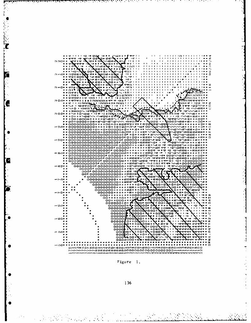
N'40 V

L0 N* ~ '~ * * *~~* * ~ I I I I 00+00+II I4

44 ~ ~ 0 +Z+ vc.OD *~O 444 l j l 113II l

00 ao +~0 *.*cc 4.0 + -T--v4 1 II It I I I i II

N. -0 VC*4 *++.4 04 -. ~ 131I III * II

11-. 1I~ 111 11 11 NI N4 11 0I ,*~~~~~ .,IC*~ii 4 *~ I IIII I N, it *, II it i

,0* 4 ~ i ii lii " I cqc*N .1I ,*-A C",'' I I N . I I I *

*1 . ~ lt +i -- +* 0IIoo 11 -0 - 11O I C1 N ~ ~ 11 1i 1 *INV *W

+ I .40 *W ( , I I -WV~~i 11 ii. 11 *1 1*'.. 2 - 4W+ 40.04+* +00.4.4.(D ... C 0 4moI#~ ii 11i~i liiTi- *~ *T 0 *- 4. . . **

00 + 0000 + .0 +00 *CPT1 wo0-'VcO.4. .400**-**000000004..00 4. . . t**o~o 0.0ow ----. ~. . . . . . 03

* 000000oo4.4..40. .. . o)D+0 O -'JI,--* *0-. . -. 00 . . . . . ..* *000000000+0++000000.0++ .4 M+. * +.-.-~ .~40 +. +

* ~~* *000000000000+.000000000*.... 4.0*-. .. *

**00000000000000000000+ 0*4+.. 4* * 00 tow -Q-C-OD34..4.4.

* *0000000000000000+00300000-4.0 * -0 :v *-4 + .~ + + S

.S* *O0000OO00000000O00*00000.. ~0....... o-4*VI .490.. . W+ 0

Or* *oOO00OO000Oo000* 0000 ... 00.4.4. W-04 * 04....4.. **.0O0O000o00o000*0000.4...+~.. -0- ...0 00

-0**0000OO0O0O(OOOD*0O000.4.4.004..00+- *.WW * *fl.w--Wo4.4.4.4.4*** *00000000000*0004. 4.44.4 4.aD~ w+~ 0-0+4.+. 4.400**

*400000000000* 0000000O0 + + 000000- .- A I N II 11,* 04., +4 4000000*.0000000000*000000004.0*0lUi *IU' ~.40000*

00000*0000000000++404. if -0- **o

000*00000000004.4.0 MW CI *4 v M* 0,00%00*000000000000+MO 30--.= **00 0004.**

** 000000000000++.4.---40+- ooc0 *0000 0000"4*00000000000.4.4.a004. OM4. 4..0 ++40 00000 0+*

** * 00000000000++O4.W0 0* 0+.40 4000* 0000.+.** 0000000000......0. 004.0 4.04.0* 04.4.0 0*4

** ~00000004..4.4004.400 *000. 004.4* 00 .-. **

0000000++4.+++Joao+4++00+. 04.* -000W-0** *000000 ... 4.4. 0+000000 +0

*4 *000.4..4...4.4.0000000 0 04.4.4.4 4* 0** *00.4..4.4.00+++.0 0 0000 4.44.4 W-0

*00+.4+000+. + 0000 ++0.0 VW0

000000.0. 0*00 *00. +.0 + -.wooTO* 0000000. * 0 00*0C *4.4.4 o.....4

#* * 00000000 00 0*04000 + (D0ww. ...... 400* oo0000 0000 000. OV-l co........*

* ~00000 000. 4.400 040...........

** 4 ~00000 0* 000. *+ +4CI W- 40.............-0:00000 000 04... **0400

** ~0000 0+4.40 000.. VW"O..o~I4I~4

* 0000 ... 4.. 04.000 40.* 0000 +. I0000 ++0.000 0*** V, *

1Wl 00 04. 4.+04.+0 * ... vv ~I*54* ~000 00. 4440 0--.C ++U~ CIO~~ WI**

*4*00000004.0 +00000 . --- vlr%. ? **T

0 rr (rtt-ljz x wommm m n cc o o oo 00 ---------- N

Figure 1

136

I.N

Figure 2

137

SATELLITE AVHRR IMAGES FOR MIZEX 84

Ola M.Johannessen, Geophysical Institute, Univ. of Bergenand Kjell Kloster, Chr. Michelsens institute, Bergen.

During Mizex-84 AVHRR-data in the form of Quick-looks and digital tapeshave been obtained through Tromso Staellite Telemetry Station. The coverage

on a daily basis is almost complete between May 07 to August 11. A datareport entitled "Satellite AVHRR Images for MIZEX 1984 Fram Strait Ex-periment" by Kjell Kloster has been printed and is available.

0

138

.I

ACOUSTICSI

139

677

MIZEX 84: SUMMARY OF ACOUSTICS PROGRAM

Arthur B. Baggeroer and Ira Dyer

The Acoustics Program was conducted using Kvitbjorn, Sverdrup, Lynchand Polarqueen plus several helicopters and fixed wing aircraft. Per-sonnel from MIT, WHOI, NRL, and NUSC participated aboard ship. Thescientific elements are sunnarized herein.

The acoustics efforts aboard Kvitbjorn centered upon use of a self-locating horizontal array drifting on the ice floes and a vertical arraydeployed from the ship. In addition, a high frequency array and a

re telemetry system for scattering measurements were deployed. The hori-zontal array could accommodate 24 channels; however, the very high rateof ice divergence prevented full deployment and resulted in 15 to 17hydrophones being operative at a time. The remaining data channelswere filled in with sensors from the vertical array. The vertical arrayoperated successfully with 28 of 30 channels; however, there is a modest

amount of ship noise on the upper channels except during the time whenthe ship power was off.

The acoustics efforts aboard Sverdrup centered upon a line array fixedto the bottom off Svalbard in open water. Some difficulty was encounteredin acquiring data from all sensors on the array, but data of high qialitvand usefulness nevertheless were obtained. Also, the program was some-what foreshortened by adverse sea conditions early in the program and byinterference from a non MIZEX ship operating close by near the end.

Lynch and Polarqueen acted as source ships for the Acoustics Program.Also Lynch deployed and recovered a source which was fixed to the bottom,and which was used for pre-tomography and transmission experiments.Acoustic transmission

Signals from the HLF-3, two mid-frequency sources, and SUS shots

deployed from the Polarqueen were recorded extensively aboard Kvitbjorn.In the early part of the experiment the Polarqueen was 40 km distant, sothe SNR was very high. After she redeployed because of the deterioratingice conditions near her she was 80-100 km distant, so the SNR was lower,

-' and more appropriate for study of long range propagation. Signals fromthe Lynch (HLF-3 and SUS shots) were recorded over a large set of rangesin her track. The signal quality was good except for the most distantranges. Two NOAA P-3 flights dropped SUS charges and made laser iceprofiles in support of the transmission experiments. The suite ofsignals recorded are over a wide range of conditions representative ofMIZ propagation.

Signals from the Lynch, Polarqueen, and the bottom-fixed source wererecorded aboard Sverdrup. A large set of transmission ranges resultedfrom the Lynch track, appropriate for study of both short and longrange transmission.

Acoustic tomography* Signals from the bottom-fixed source were recorded on both the hori-

zontal and vertical arrays at Kvitbjorn. A special system for the tomo-graphy signals, the DIBOS recorder, did not function properly.Fortunately, the digital system and analog system recording bandwidths

140

S ~i|. . lllll° a llellll

cover the frequency band, so data can be recovered from them.Seismic refraction and acoustic impulse response

Three lines, two along the crest of the Yermak Plateau and one normalto it, were shot with I km spacing to offsets of 20 km, and recordedaboard Kvitbjorn. There was not enough ice for landing the helicopter topermit shooting reversed lines. SUS charges were also deployed duringthe seismic refraction lines for impulse response measurements. Theselines were supplemented with two additional ones solely for impulseresponses.

Seismic refraction lines near Sverdrup were not successfully recorded.The shot sizes were too small to overcome noise at long ranges and toointensive for the recording dynamic range at short ranges.Seismic reflection

Three days of seismic reflection with a 40 cu in air gun were done fromthe Kvitbjorn. Only 3-5 sensors were then active because the Kvitbjornhad to reenter the ice edge after drifting into open water. The drifttrack during this phase overlapped parts of the seismic refraction lineson the Yermak Plateau.Ambient Noise

Extensive recordings of ambient noise were done both at the Kvitbjornand remotely via helicopter and sonobuoys. The recordings at the Kvit-bjorn were done by turning off the ship's power and running solely on a12 kw generator. Both horizontal and vertical array sensors were used,

* so angular dependencies can be determined for frequencies below 250 Hz.Wideband ambient noise data to 2 kHz were recorded on analog tapes, andspectral samples to 50 kHz were measured in real-time. Remote measure-ments were made by installing a spectrum analyzer, tape recorder andplotter on the helicopter and powering them with a small generator.Point measurements were made along the ice edge and normal to it forranges of 80 km from the Kvitbjorn. Three Norwegian P-3 flights using57A sonobuoys were also used to record ambient noise data. The crewindicated that "high quality" recordings were obtained. Ambient noisewas also recorded aboard the Sverdrup.Reverberation and backscattering

Three 100 kg explosions for measuring low frequency reverberation andice backscattering were deployed and recorded successfully aboard theKvitbjorn under quiet ship conditions.Acoustic telemetry and hf scattering

Two sets of 50 kHz acoustic telemetry data over 1 km range were re-corded at the Kvitbjorn. These data will be useful in characterizingice effects on hf acoustic signals as well as on performance of thetelemetry system beneath the ice canopy.Ice kinematics by acoustics

The self-locating capability of Kvitbjorn's horizontal array providedtracking of the ice from individual sensor motion. See attached figuresfor a tentative result. Headings and fixes were logged concurrently soabsolute positions can be estimated to within rotation of the array; how-ever, during periods of rapid motion the sampling may not be adequate.Radar reflectors were not effective and the sensors were often not invisual distance of the ship, thus eliminating a useful check.

14 1411

00

0

z

C InUn

H

00Z

Q D

-II

-5800 MIZEx 84 Fat 86 .16,84 e :59:14 580

DISTANCE WEST OF KVITBJORN (M)

Sensor positions determined in real time June 16, 1984during the MIZEX 84 experiment. Kvitbjorn is in groupof sensors near bottom of plot.

14

142

0I• •.

. . . -- +- "o,,, b ,, ,,-,, , u ~ am, ll m+ du m I ~ m . -

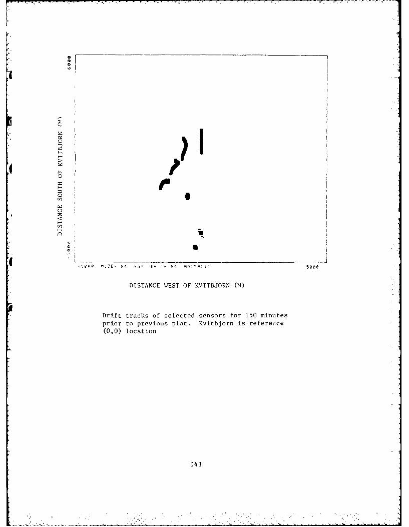
47

z >'F-

E E!tE 0 4 1p 41DITNEWS F VTJR M

Drif trcso eetdsnsrUo 5 iuepro opeiu lt Kiboni eeec

(0,0 loctio

F143

I

MIZEX 84 CRUISE REPORTKVITBJORN: FIRST LEG 2 June - 30 June

IRA DYER

MIZEX 84 in overall was a complicated operation, entailing a largenumber of scientific objectives, scientists, ships and aircraft.Kvitbjorn's role was largely related to acoustics, which required closecollaboration with Lynch, Sverdrup, and Polarqueen, and with severalhelicopters and fixed wing aircraft. Kvitbjorn also included smallerprograms in oceanography and meteorology. Coordination of Kvitbjorn'sprograms with the larger objectives of MIZEX 84 showed daily evidence of

difficulties and irritations, but it is a credit to Ola Johannessen andhis management team that MIZEX 84 worked. If there is a simple formuladescribing this positive outcome, it would relate to detailed planning,dedication to scientific objectives, flexibility under constraint, andmutual understanding.

The at-sea communications burden was immense, but necessary. Thisburden entailed much more than the Acoustics Program; indeed it can besaid that radio communications with the Kvitbjorn involving strictlyacoustics science was much smaller than communications involving theremainder of the program. The time budget each day on average wasapproximately: - 0500 voice reporting: 2 hours

- 1900 voice reporting: 1 hour- 2000 Telex reporting: 2 hours

To this budget we should add approximately 1 hour/day for miscellaneousvoice communications with other ships on special operational orscientific questions. Thus, about 6 hours per day were devoted to radiocommunications, requiring one of our senior staff to be on the bridgeinstead of attending to science.

Aircraft operations placed a large additional burden on our staff,since helo operations entailed continuous radar andradio contact.Kvitbjorn's helo averaged 4 hours/day of actual flying time plusat least 4 hours/day of remote on-ice ti-e (that is, with the helo shutdown at a remote station while instruments were deployed, maintained,data taken, etc.). Thus one of the staff also had to devote an averageof at least 8 hours/day of bridge time to keep the helo going. Coupledwith this were frequent overflights of the NOAA-P3, the Norwegian P3,the CV-990, the CV-580, the Falcon, and other helos from the Polarqueen,Polarstern, and Svalbard. Fortunately most of these other flightsoccurred when Kvitbjorn's helo was operating, creating no additionaltime burden on our staff. Unfortunately, none of us was really pre-pared for air-traffic control work; we now know first-hand why manycontrollers develop ulcers and nervous breakdowns.

In retrospect we should have had a PSC logistics person with us totake on the 14 hour/day burden of radio communications and air trafficcontrol. As it turned out, this burden affected the science programthrough inadequate rest, and through less real-time reduction of datathan we would have liked.

144

6l

4J

Navigation data for the first leg of Kvitbjorn are summarized in theattached figures, and cover Julian day 157 (5 June 1984) to Julian day182 (30 June 1984), which go from the first in-ice day to the return to

SLongyearbyen for rotation and resupply. Position data were initiallyobtained by hand logging of the ship's satellite navigation receiver,and linearly interpolated. At Julian day 171 another receiver wasbrought on line which could be logged directly by our computer.

In brief, Kvitbjorn occupied several drift stations during the leg.I As the position data show, the general drift direction was south whicha put us at times too close to the ice edge or at a position of too low

ice concentration. The need to move back to better ice conditions,requiring recovery and then redeployment of equipment, caused inter-ruptions in all Kvitbjorn science programs. Further, since Kvitbjorndoes not have a helo pad, we depended upon adjacent ice floes as pads,which caused additional logistic delays during repositioning. (During

[f one repositioning Kvitbjorn proceeded slowly north, dragging the helo'sice pad with us.)

We elected to rotate science crews by transit to Longyearbyen,rather than via Svalbard helicopter as originally planned. The under-lying rationale for this change was the desire to occupy CTD stationssouth of the ice edge to assist in measuring an eddy which had been

* discovered by others. (We also took this opportunity to deploy XBTswhile underway and to continue float tracking while on station.) Ship'sresupply as well as crew rotation was simplified by this change.

On balance, Kvitbjorn's capabilities served us well. A larger shipcould have punched further into the ice. But a larger ship would haveentailed )rograms interferring with quiet ship requirements. Quiet ship

Centailed siut down of all ship's machinery. A specially isolated motorgenerator supplied power for the acoustics' equipment.

Kvitbjorn's skipper and crew supported us with enthusiasm and skill.They genuinely seemed to enjoy the challenge of our mission compared tothe usual routine of fishing, and they creatively improvised mechanicaland/or electrical solutions to our many shipboard problems. And sinceit can be said that Arctic experimentors rely as much on their stomachsas their heads to get good data, Kvitbjorn's cook and stores served usexceptionally well.

The helo pilot and mechanic also supported us with enthusiasm andskill. Because flying weather rarely was a detriment, the helo wouldfly whenever we needed to even though the duty time might have stretchedwell beyond normal. (We never violated the limit of 8 hour/day flyingtime; duty time would go beyond 16 hours on many days.) The pilot waseager as we were to get on with our science.

The Kvitbjorn was well served by PSC in Tromso prior to departure,at sea in arranging for special delivery of replacement navigation andradio equipment, and in Longyearbyen upon return. Tromso served as avaluable shore-based radio contact for operations, for reporting, and

for weather forecasts during the leg.

145

16 S

,JLA A

Fi.1 iesre fltiuepstolnalinepltd

14

14

L . ., . . . . .. -, ..r.. . 7 .. . . -. -

I

Vertical Array Acoustics

Ronald L. Dicus, US Naval Research Laboratory, Washington DC, 20375

The time/space coherence of underwater sound propagating in the Marginal IceZone (MIZ) is degraded in part by scattering from the underside of rough icefloes. In the MIZ the nature of the underice surface is highly variable both

temporally and spatially. Although other characteristics of the propogationchannel such as the multipath structure, the ocean bottom, and time/spacefluctuations of the sound-velocity profile may be expected to contribute to

coherence losses, the Naval Research Laboratory (NRL) has as its primary

objective to focus on the acoustic ice interaction and in particular thoseaspects that may be measured with a vertical array. To pursue this objective

NRL deployed a vertical array from M/S KVITBJORN during the period fromJune 13 to June 24. The array consisted of 24 hydrophones attached to akevlar strength member and suspended at depths from 24 to 313 m. The phoneswere spaced for an overall aperture at 30 Hz plus two nested subapertures at

400 HZ and 800 Hz. The individual hydrophone depths are listed in Table 1.Hydrophone number 24 became operational on June 17. The top-most hydrophone

failed on June 19, probably due to a catastrophic encounter with an ice floe.Signals were recorded on a 32-track analog Sangamo Sabre V machine using 14inch reel, 1 inch wide, 1.5 mil thick magnetic tape. Frequency response wasfrom 5 Hz to 3000 Hz. Preamplifier and postamplifier gain switches permitted

recording levels from 90 dB to 127 dB re 1 uPa, which includes ambient noiselevels and signal levels well beyond the peak pressure of a Mk-61 SUSexplosive charge (1.8 lb) at 1 km range.

The approach was to measure short range and long range explosive charge and

projector signals. As part of post-experiment processing, explosive charge

signals and broadband projector signals will be beamformed and deconvolved(to remove source signature effects) to extract the vertical directional

impulse response of the ice. Narrowband projector signals will provideinformation on transmission loss and arrival structure. The space/time

coherence of the beamformed signals will be studied as a function of timeand ice conditions and as a function of range and frequency. Quantitative

measures of ice conditions will be based on remote sensing data such asphotography, laser profilometer and microwave passive imagery as provided

by other MIZEX participants.

Explosive shot signal sources were deployed from helicopter and P-3 aircraft

along radial tracks centered on the vertical array. Details of the shot data

collected including date of the event, track bearing angle, source ranges andtype of explosive (main charge weight and detonation depth) are summarized inTable 2. Narrowband and broadband programmed projector signals originating

from POLAR QUEEN and LYNCH were recorded. Dates and hours during which these

signals were recorded from the vertical array are summarized in Table 3.

An example of a short range shot signal is shown in Fig. 1. The first

positive going spikes are the direct path shock and bubble pulse arrivals.

The second arrival packet is the ice reflected energy. The Ice reflected

pulses are attenuated and show additional high frequency tails. An example

148

I

t77

of narrowband signal energy is shown in Fig. 2. This is the 110 Hz linetypical of transmissions from the LYNCH HLF-3 projector. In this case thesignal-to-noise ratio (SNR) is high; however, the SNR was quite variable anddepended on source range, ice conditions, and the ambient noise. A typicalambient noise spectrum is shown in Fig. 3. The top curve is for the usualstation keeping duties of the ship; the lower curve was measured during"quiet ship" conditions when all ship generators and machinery were turnedoff. Thus, ship noise contributes significantly to the observed noise back-ground as expected for hydrophones suspended close to the ship, and shipinduced noise is of course characterized by strong lines. Another source ofstrong lines below 50 Hz is due to strumming as shown in Fig. 4. The dashedcurve was measured on a day when there was no strumming; the solid curvefrom another day shows the strong, narrow strumming lines. Strumming wasobserved mainly on days when the ice floes were separated by large open waterareas and the ship's drift velocity was high.

The data set is of the quality and breadth to satisfy the processingobjectives of the experiment. In spite of the noise sources shown abovemost of the short signals were at a high level relative to the noise, andfor narrowband processing most of the projector lines fall by chance betweenstrong noise lines. For example, the background noise measured at one timefor 100 Hz and 300 Hz was approximately 72 dB re I uPa/Hz, a level not muchhigher than the expected ambient noise level. After all shot runs werecompleted and all projectors had been shut down the vertical array continuedto record air-gun signals which will provide information about the bottomenvironment. In all, some 370 shot signals and 105 hours of projectorsignals were successfully recorded.

14

149

_ _ _ .1

-.- J." - -

L

Table 1. Deployment depths of hydrophones.Sequence 1 2 3 4 5 6 7 8Phone ID 4 6 7 8 9 10 11 12Depth(m) 24.4 72.4 96.4 120.4 144.3 168.3 192.3 216.3Sequence 9 10 11 12 13 14 15 16Phone ID 13 14 15 16 17 18 19 20Depth (m) 240.3 264.3 288.3 297.9 299.7 301.5 302.4 303.3Sequence 17 18 19 20 21 22 23 24Phone ID 21 22 24 25 26 27 28 29Depth (m) 304.2 305.1 306.9 307.8 308.7 309.6 311.4 313.2

Table 2. Explosive charge deployments.-" Date Aircraft Bearing Max range Type of Charge

(degrees) (km) Weight(kg) Depth(m) Range(km) Number6/16 Helo 320 19 0.82 91 4-19 21

0.82 244 1-19 2010.0 244 4-19 17

6/17 Helo 50 22 0.82 91 4-22 190.82 244 1-22 23

10.0 244 4-9 625.0 244 10-22 9

6/18 Helo 0 46 0.03 244 0.5-5. 8* 0.82 91 0.5-46. 20

0.82 244 0.5-46. 196/10 Helo 25 47 0.82 91 0.5-47. 17

0.82 244 0.5-47. 166/21 ilelo 320 33 0.82 91 1-33 15

0.82 244 1-33 1910.0 244 4-8 425.0 244 9-33 11

6/22 P-3 270 400 0.82 244 1-50 11315 0.82 244 1-50 11

0 0.82 244 -lO0to+400 1945 0.82 244 1-50 1190 0.82 244 1-50 11

6/24 P-3 270 400 0.82 244 1-50 11315 0.82 244 1-50 110 0.82 244 -lOOto+400 19

45 0.82 244 1-50 1190 0.82 244 1-50 11

Table 3. Hours during which projector signals were recorded.Date Hours (Zulu Time)14 0948-1335 1515-1603 1645-190015 0956-1130 1154-154816 1907-2400

* 17 0000-1057 1552-182618 0615-1030 2358-240019 0000-0003 0150-0900 0917-1200 1255-1600 1624-1800 1852-240020 0000-0400 1023-125522 1255-2136 2150-240023 0000-0200 0211-0425 0432-1200 1229-2030 2330-2400

* 24 0000-0521 0530-0900

150

-60

p,0

U° w -60 -

-70

-900 0.05 0.10 0.15 0.20 108 109 110 111 112

Time (sec) Frequency (Hz)

Fig. 1. Shot signal at 0.67 km Fig. 2. Projector signalrange. Explosive charge: 0.82 kg from HLF-3 source aboardat 244 m depth. US LYNCH. Analysis band-

width 60 mHz.

6i

-20

.40 -40-606 0 -50

Q)-7 0

•J-60F -80 , n -70

0 100 200 300 400 500

Frequency (Hz) -800 10 20 30 40 50

Fig. 3. Measured noise spectrum. Frequency (Hz)Lower curve is for "quiet ship" Fig. 4. Measuredconditions. noise spectrum with

strumming - and

without---.

4

1

151

CTD and Deployment Activities Aboard USNS LYNCH During First Legof NRL Cruise 707-84 for the Marginal Ice Zone Experiment

Charles W. Votaw and Stephen C. Wales

During May and June of 1984 the USNS LYNCH participated in ONR'sMarginal Ice Zone Eperiment (MIZEX) in the Fram Strait and northernGreenland Sea. This cruise was composed of two legs during May and Junerespectively. During the first leg the LYNCH deployed an acoustic source,transponders, current meters, and surface drifting bouys; recoveredcurrent meters; and made CTD measurements along a transect across the FramStrait. During the second leg the LYNCH towed the HLF-3 acoustic source,recovered the acoustic source and a transponder, and made XSV, CTD andmeterological measurements. It also made cavitation measurements for anon-MIZEX project. This article summarizes the COD and deployment activitiesduring the first leg of the cruise. The reader is refered to other articlesfor an in-depth description of the purpose of each of these experiments andtheir coordination with other facets of MIZEX.

The princopal objective of this leg was to make a large number ofinstrument deployments in support of MIZEX. These deployments with approx-imate positions are summarized in Table I. The first deployments scheduledwere for the Wood's Hole Oceanographic Institute's (WHOI) moored acousticsource and its three position transponders. These were successfully deployedas scheduled. During the second leg the source and one transponder wererecovered. The source operated successfully throughout the experiment.

The LYNCH was next scheduled to recover a University of Washington (UW)current meter mooring C-8, but it was decided to delay the recovery untilafter other deployments to provide some badly needed deck space. UWmoorings FS-7 and FS-8 were deployed next. Following this the Lamont-Doherty Geological Observatory's (LDGC) 1983 mooring was recovered. The nextset of deployments scheduled were for the LDGO triangular array ofcurrent meters at the ice edge. These deployments required that the

*R bathymetry, line streach, and the deployment dynamics be known to highprecision so that the current meter would be at a very shallow depth. Fourattempts were made to deploy the current meter strings in this triangle,only one of which was successful. Because of the difficulty of cutting theline on the deck, necessitated by an uncertain position of the ice edge, asopposed to premeasured lines, three of these moorings turned up with the

* subsurface floats floating on the surface. The unsuccessful attempts wererecoved so no equipment was lost.

During the attempts at launching the LDGO current maters, two of theARGOS bouys from Laboratoire D'Oceanographie Physique were deployed alongthe ice edge. These were originally scheduled to be deployed along the

* northern ice edge but were deployed in this location due to tine constraints.See Table I.

Following the LDGO current meter work a CTD transect was made of the IFram Strait. Beginning near the ice edge at 78 551N, 0 30'E CTDs were takenevery degree in longitude to 7 30'E, or just over 10 nms apart and half

* degree spacings thereafter to 9 30'E. Other CTDs were taken near the ice

152." I,* .

° • . - . - . - . .- - -_

edge and in the vicinity of the WHOI source. A total of 15 CTDs were takenthroughout the first leg. The third ARGOS bouy was deployed near theEastern end of this transect.

Following the CTD transect scientific operations were interupted fornearly two days due to rough weather. On the afternoon of the 27th,operations resumed with the final current meter deployments and recovery forUW. Current meter strings FS-6, FS-5, and FS-4 were successfully deployedand the previously deployed current neter C-8 was recovered.

Satellite navigation was used through out the cruise and positions wererecorded and at every satellite fix. LORAN-C was found to be unsatisfactoryat these latitudes. Bathynetry was recorded throughout the leg on both3.5 kHz and 12 kHz recorders.

I

I

a]

-1

.4

153 "

4

Table I - Approximate Deployment Locations and Times

Time Deployment(GMT) Positions

Wood's Hole Ocean. Inst.Moored Source 21 May 0655 78 59.3'N 6 58.6'ETransponder #1 21 May 0847 79 00.0'N 6 58.6'ETransponder #2 23. May 0922 78 59.1'N 6 51.2'ETransponder #3 21 May 1002 78 59.0'N 7 12.0'E

Univ. of Wash.Current meters FS-4 28 May 0305 78 39.0'N 4 05.0'ECurrent meters FS-5 27 May 2248 78 42.8'N 5 33.9'ECurrent meters FS-6 27 May 1714 78 40.2'N 6 19.6'ECurrent meters FS-7 21 May 2021 78 53.7'N 8 05.2'ECurrent meters FS-8 22 May 1256 78 04.3'N 3 46.1'E1983 meters C-8 28 May 0830 Successful recovery

Lab. D'Ocean. Phys.ARGOS bouy #5092 23 May 1135 79 18.6'N 1 54.8'EARGOS bouy #5087 23 May 1300 79 20.2'N 3 00.8'EARGOS bouy #5096 25 May 1012 78 56.4'N 7 37.0'E

Lamont-Doherty Geol. Obs.1983 current meters 22 May 1800 Successful recoveryCurrent meters #1 23 May 0254 (See text)Current meters #2 23 May 2144 78 46.3'N 0 10.2'ECurrent meters #3 24 May 0228 (See text)

In addition Lamont-Doherty took 15 CTD measurements along the ice edge andalong 78 55'N frcm 0 30'E to 9 30'E in 1 degree intervals.

0

154

0

HLF-3 acoustic source activities aboard the USNS LYNCH during

NRL Cruise 707-84 for the Marginal Ice Zone Experiment

r Stephen C. Wales, U.S. Naval Research Laboratory, Washington, D.C. 20375

During May and June of 1984 the USNS LYNCH participated in ONR's Marginal IceZone Experiment (MIZEX) in the Fram Strait and northern Greenland Sea. Thiscruise was composed of two legs during May and June respectively. During the

second leg, discussed here, the LYNCH towed the HLF-3 acoustic source, recov-ered the acoustic source and a transponder, and made XSV, CTD and meterological

*measurements. It also made cavitation measurements for a non-MIZEX project.This article describes the HLF-3 and XSV activites aboard the LYNCH during the

second leg. While this section includes some indication of the other activitesaboard the LYNCH, the reader is refered to other articles for an in-depth

description of them.

On arriving in the operation area the LYNCH began deploying the HLF-3 source at2100 Z on 8 June after encountering ice. The deployment went very smoothly and

the source was in and operational within two hours. The source was turned onat 0000 Z 9 June and the LYNCH began sailing her scheduled tracks. The LYNCHwas generally able to pull the source comfortably at 7.5 knots, under goodconditions she made 8 knots and in rough weather the speed dropped to 5.5

* knots. 3ource waveforms were broadcast as directed by the source schedule [Il]

with only a few minor variations due to operator error or routine source main-tenance. The source worked flawlessly throughout the experiment.

The towing tracks were generally as intended. However, ice was encounteredrepeatedly along the northern and western legs in unreported positions, and

athis required that these tracks be restructured to avoid the ice. This wasexpected during the planning phase due to the uncertainty in ice location.Figure I shows the tow tracks followed by the LYNCH. Tracks were also changed,at the request of SVERDRUP, to avoid the immediate vicinity of the SVERDRUP and

to obtain more time between the northern region between SVERDRUP and KVITBJORN.

The final circuit to the south was shortened to accommodate the latter change.

BReginning on the evening of 12 June the LYNCH was accompanied by the Soviet

ship SENEZH. The SENEZH stayed with the LYNCH throughout her operations onlyleaving her when she was well on her way to Reykjavik after the experiment.

With one exception, she did not interfere with the LYNCH's operations.

* The HLF-3 source was recovered near the WHOI moored source's location without

problems at 0700 Z 19 June, slightly ahead of schedule. The moored source wasthen recovered, but due to worsening weather no attempt was made to recover the

transponders at that time. The LYNCH then proceeded north to the ice-edge andbegan her participation in the synoptic CTD survey. She accomplished two ofher three scheduled legs and the NORDA cavitation work before breaking off for

* another attempt at recovering the transponders.

After returning to the WHOI moored source site the transponders were locatedand released, one at a time. The first transponder was recovered by the SENEZH,the second was lost, and the LYNCH recovered the last one. After this, theLYNCH redeployed the HLF-3 source AT 1300 Z 22 June and began a final tow at

* 1430 Z to the southwest along a previous track. She recovered the source at

155

.7

0530 Z 24 June and arrived in Reykjavik, Iceland on 28 June where the scien-

tific personnel disembarked.

During the experiment the source was monitored by the scientific personnel atall times. Source information was recorded on 7-track analog tape at 15/16

( ips, in IRIG Wideband Group I format, according to Table I. The FM bandwidthis 625 Hz. Source operations were also recorded in a written log by time, withwaveform type, input, depth, sea temperature, and hydrophone and accelerometervoltages recorded hourly. Additionally, spectrum plots, taken everytime the

source waveform was changed, and a six-channel brush recorder provided a visualdisplay of the information being recorded.

42 Mark 61 SUS charges, 1.8 lbs TNT with a 1.1 oz tetryl booster, were dropped

from 1245 Z 12 June to 1015 Z 13 June at half-hour intervals, 3 were duds. .

P11 charges were set for nominally an 800 ft depth. Drop time, detonation

time and position were logged for each drop. The difference in the times will

provide the actual shot depth.

24 Sippican expendable sound velocimeters, XSV-02s, were dropped during the

cruise. Along with CTD information taken from the LYNCH and other ships, theseare expected to provide the necessary sound velocity information to interpretthe acoustic data. The XSVs were dropped in a pattern intended to cover theentire LYNCH towing area concentrating more on the northernmost region wherethe sound speed profile was most rapidly changing. There were an insufficient

number of XSVs to duplicate locations and look for sound velocity variablity,however one XSV was dropped at the same location as a CTD measurement. Agree-

ment as judged from the thermal printer plot, was very good. The signals fromthe XSVs were recorded on 4 cassette cartridges using an Hewlett-Packard IIP-85

personel computer and a Sippican Mark 9 interface box.

Satellite navigation was used through out the cruise and positions wererecorded every half-hour and at every satellite fix. LORAN-C was recorded onthe quarter-hours and was found to agree with the satellite fixes at the lowerlatitudes. Bathymetry was recorded throughout both towing phases and enrouteto the operations area on both 3.5 kllz and 12 kHz. During the synoptic survey

* period the 12 kHz transducer was used with the CTD device and the 3.5 kHztransducer was under repair.

Acoustic operations aboard the LYNCH went nearly flawlessly during MIZEX andall major acoustic goals aboard the LYNCH were accomplished. MIZEX partici-pants who have questions concerning the HLF-3 source data, XSV data, naviga-

4 tion, or bathymetry, should contact the author. The author would like to thankthe officers and crew of the LYNCH and the members of the scientific party whomade this a particularily smooth cruise. Special thanks are in order to theindividuals who made the acoustic operations work, E. Daniel McCloskey ofHydroacoustics, Inc., John Kemp of Wood's Hole Oceanographic Institute, HaroldWare of the Naval Underwater Systems Center, Rubin Naber of the Naval Research

* Laboratory, and James Hannon of Sippican Inc., which loaned us the Mark 9 box

and the HP-85.

1. F.R. DiNapoli, "Corrections to LYNCH HLF-3 Towing Schedule" 401Y-34, April24, 1984, and encls. "MIZEX-R4 LYNCH HLF-3 Towing Schedule; mod-3," 401Y-16,

and "Proposed MIZEX-84 transmission schedule for POLAR QUEEN, mod-l," 401Y-32,* Naval Underwater Systems Center, New London Conn.

156

6J

80

79

78

J /

77 \

( ~~ ~ ~~76 ij/ // .-

I z A

-10 -5 o 5 s 15

*Longitude

Figure 1. HLF-3 source tow tracks by the USNS LYNCH during MIZEX, 9-24 June1984, in the Fram Strait. Dots indicate starting and ending points, arrowsthe ship's direction.

Table I - Recorded HLF-3 source information

Item Tape Ch. Mode Brush Ch. Comments

Tach Signal I Direct -

Clock (IRIG-B) 2 Direct 3 On brush as slow codeSource input waveform 3 FM 1 Add 10 dBHydrophone waveform 4 FM 2 -184.8 dB/volt/pPa

Accelerometer 5 FM 4 3.12 's/v, varies with frequencyDepth 6 FM 5 68 m/voltSea temperature 7 FM 6 100 C/volt

157

E

ACOUSTIC TOMOGRAPHY SOURCE

Robert C. Spindelt Woods Hole Oceanographic Institution

An autonomous, moored, acoustic transmission consisted of a contin-source was deployed on Leg 1 of the uous repetition of this sequence;USNS Lynch in May, 1984, to assess the hourly 3 minute transmissionsthe stability of surface reflected consisted of 48 repetitions.acoustic paths for tomographic ap-plication. The source transmitted a The source mooring was equipped with224 Hz carrier, phase modulated by a a system to measure the position ofbinary, maximal-length shift-reg- the source as the mooring moved inister sequence, similar to the type response to tidal and other forcingof signal transmitted during several currents. An acoustic interrogatortomography experiments. Minor ad- measured the slant range to threejustments in signalling parameters transponders in an equilateral tri-were made to account for Doppler angle about the base of the mooringshifts due to the time-varying ocean at a distance of about 1 km from thesurface. The signal was received by mooring anchor.hydrophones suspended through theice by the MIT/WHOI scientific party The status of data return is veryaboard the MV Kvitbjorn and by hy- preliminary. The source signal wasdrophones deployed by the HU heard on Sverdrup hydrophones and itSverdrup. is assumed that successful record-

ings were made. The signal wasThe source was moored at a depth of recorded on a special digital re-175 meters in 1207 meter (corrected) ceiver connected to a Kvitbjornwater at 78059:3 N, 6058:6 E. It hydrophone, but there has been somebegan transmitting at OOOZ on problem reading that instrument'sJulian day 161 (9 June) and ceased tape and it is not yet certainat OOOOZ on day 171. The trans- whether it will be successfullymission sequence consisted of two read. The signal was also recordedhours of continuous transmission by the MIT/WHOI acoustic array.starting at OOOOZ each day, and These tapes have not yet arrived inapproximately 3 minutes of trans- the U.S. and, therefore, their qual-mission at the start of each hour ity has yet to be evaluated. How-beginning at 0300Z and lasting ever, since there is triple redun-through 2300Z. The binary sequence dancy in data recording the expec-consisted of a 63 bit code, with 14 tation of successful data return iscycles of the 224 Hz carrier per high.digit. Each digit modulated thecarrier +/- 82.82 degrees depending Analysis of the data with respect toon whether the digit was a zero or a tomography application is scheduledone. This modulation angle results for late 1984 and early 1985.in maximum signal-to-noise ratio forthe particular signal parametersused. The total transmission timefor an entire binary sequence was 63bits x 14/224 seconds/bit = 3.9375seconds. The once daily two hour

158

6L

SCIENTIFIC ACTIVITIES ABOARD H.U.SVERDRUP

F.R.DiNapoli, NUSC,Code 01Y

NUSC deployed a long bottomed array at approximately 80 N and 7 E on June 9utilizing the Norwegian Defense Research Establishment vessel H.U.SVERDRUP.Acoustic signals were recorded from the acoustic source towed in openwater by the Lynch and from another source suspended from the POLARQUEENin the MIZ from June 9 to June 19.

On June 19, the Soviet AGOR "SENYEZ" cut the mooring line to the surfacetelemetry buoy. A second line from the surface buoy to the bottomed array

*° was broken by heavy seas shortly after the interference by "SENYEZ" and4( the experiment had to be prematurely terminated.

The SVERDRUP then obtained sound velocity versus depth measurements on atrack from the site to the position of the POLARQUEEN.

The overall quality of data collected was generally good, but we did ex-perience the following difficulties:

o A failure of unknown origin prevented us from recording datafrom the full aperture;

o Severe strumming on the short vertical portion of the arraymade that data totally unusable;

o Data from the refraction run was contaminated by SVERDRUP's ownship noise.

A total of 240 hours of data were obtained during the experiment. A re-view of hourly in-situ ambient noise measurements show that the averageambient noise has approximately a 10 db spread and an average value whichis rather high. We suspect that this high ambient noise may be due toshipping, but the number of ships observed in the vicinity of the SVERDRUPposition was not high.

159

BIOLOGY

161

-7.-

LIFE CYCLES AND SECONDARY PRODUCTION OF DOMINANT COPEPODS

H.J. Hirche and R.M.Bohrer

Life cycles and secondary production of dominant herbivorous copepods werestudied during 5 mesoscale transects in the MIZ, 3 Large Scale Oceanographytransects and an eddy tracking. Three different approaches were used:

1. Egg production: The egg production of female Calanus finmarchicus andCalanus glacialis is strictly correlated with food supply. Since thefemales are not growing in this stage, egg production can be taken as ameasure of their net production under observed nutrient conditions.

4Healthy females were selected from bongo net hauls (500 um and 700 urmesh size) from the upper 150 m. The nets had closed cod ends to preventdamage to the animals.

With C. glacialis 20 experiments were carried out on 11 stations duringLarge Scale Transects. This species is found almost exclusively under theice. Eggs were produced only on stations on the Eastgreenland shelf.

With C. finmarchicus 120 experiments were done on 57 stations. Stationswere closely spaced in the MIZ and during eddy tracking. According to thehydrography and phytoplankton abundance egg production showed steepgradients in the MIZ. In general egg production was low under the ice.Maximum production was found in the MIZ, the position of the maximumdepending on the front. Towards the open Atlantic egg production appa-rently decreased.

In the laboratory the influence of experimental condition upon eggproduction was studied. Females were incubated in ambient seawater infiltered seawater and also in algae cultures. In addition maximum eggproduction was studied at different temperatures and optimum foodconditions (algae cultures).

2. Digestive enzymes: The activities of the digestive enzymes amylase andtrypsin give an indication of the physiological condition of copepods.

Our special interest focused on the overwintering stage, when the animalsreduce their metabolism and stop feeding. More than 100 homogenates ofthe copepodid stage V (CV) of Calanus finmarchicus, C. glacialis and C.hyperboreus were prepared from 500-200 m and from surface tows. Thesehomogenates are being analyzed in the laboratory.

162

4

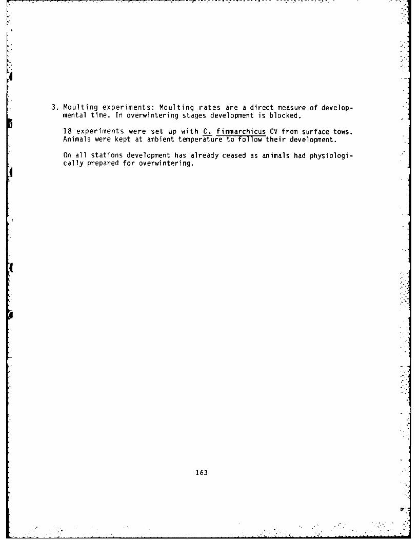
L

3. Moulting experiments: Moulting rates are a direct measure of develop-mental time. In overwintering stages development is blocked.

18 experiments were set up with C. finmarchicus CV from surface tows.Animals were kept at ambient temperature to follow their development.

On all stations development has already ceased as animals had physiologi-cally prepared for overwintering.

1

I

163-"

Ni' r 1 : itni,"j in t ho r roarIng , odge of the aist Greenland Sea

Walker 0. Smith, Louis A. Codispoti and Sharon L. Smith

During MIZEX-84 our group conducted experiments designed to assess thedistribution of nitrogen (nitrate, ammonium, urea, particulatenitrogen, zooplankton nitrogen), rates of nitrogen assimilation andturnover (nitrate, ammonium and urea uptake by phytoplankton;zooplankton excretion of ammonium and urea; ammonium regeneration by

bacteria and microzooplankton) and causal mechanisms of the ubiquitous- subsurface ammonium maximum we observed in the study region in 1983I (Smith et al., submitted). To characterize the nutrient, phytoplankton

and zooplankton fields within the marginal ice zone, discrete water .1samples were taken at stations in the MIZ from depths corresponding toE known percentages of surface radiation or from standard depths.Generally samples were analyzed through 150 m. Zooplankton weresampled by an electronic opening/closing nets (mesh size 303 um) toestimate the macrozooplankton biomass from 0-25, 25-50, 50-100,100-200, and 200-500 m. Vertical bongo tows from 0-100 m were alsoconducted to collect animals for experimentation. Chlorophyll wasmeasured to quantify phytoplankton biomass at sea. A total of 59stations were completed in which the nutrient and phytoplanktondistributions were both analyzed; zooplankton biomass was measured at48 stations.

Nutrient (nitrate, urea and ammonium) and carbon uptake were measuredusing 15N- and 14C-isotopes. Samples from 33 stations were incubatedin an on-deck incubator cooled to surface seawater temperatures inbottles fitted with neutral density screens designed to reduce thelight intensity to that of the depth sampled. Ammonium regeneration bybacteria and microzooplankton was estimated at 18 stations using an15N-NH 4 isotope dilution technique (Harrison et al., 1983).Macrozooplankton excretion rates were estimated by placing recently

collected animals in 125 ml of filtered seawater and measuring thechange in ammonium and urea concentrations after an incubation at 10C. A total of 27 macrozooplankton excretion experiments werecompleted.

Most of our data are presently being analyzed, but preliminary resultsindicate that the large spatial/temporal patterns in nitrogen(dissolved and particulate) distributions that we observed in 1983 were

- . also present in 1984. For example, ammonium showed a distinctsubsurface maximum (Figure 1) and the concentrations detected weresimilar to those found both last year and in the Bering Sea (Saino et

* al., 1983). We do not at this time understand the role of the marginalice zone in the initiation and maintainance of this feature.Phytoplankton biomass as measured by chlorophyll also showed a distinctsubsurface maximum (Figure 1) which seemed to be related to thehalocline created between the meltwater and more saline waters of NorthAtlantic origin. The spatial variations of chlorophyll also varied

* widely within the marginal ice zone (Figure 2). The data presented inFigure 2 are those collected in the first mesoscale grid survey.

164

0".

Nitrogen dynamics in the retreating ice edge of the East Greenland Sea

Walker 0. Smith, Louis A. Codispoti and Sharon L. Smith

Chlorophyll levels were extremely low in regions of heavy ice coverand increased markedly at the ice edge. There is some indication thatchlorophyll concentrations were beginning to decrease away from theice. Measurements taken simultaneously onboard the F.S. VALDIVIA willclarify this distribution.

Zooplankton were dominated by the copepods Calanus finmarchicus, C.hyperboreus and Metridia longa. Also found were Calanus glacialis andPseudocalanus spp. Although quantitative data are as yet unavailable,zooplankton were noticeably concentrated in the upper 25 m of the watercolumn. Preliminary evidence indicates that C. finmarchicus copepodids(stage V) may have already entered diapause during the study.

Much work remains before we fully understand the roles of each group oforganisms in the formation of the subsurface ammonium maximum, as wellas its relationship to the marginal ice zone. Hopefully the data wecollected will enable us to appreciate the role of nitrogen as acontrolling mechanism in the ice edge system of the East GreenlandSea.

Research sponsored by the Office of Naval Research and NSF grantDPP-8319470.

ReferencesSaino, T., H. Otobe, E. Wada and A. Harrison. 1983. Subsurfaceammonium maximum in the northern North Pacific and the Bering Sea insummer. Deep-Sea Res. 30: 1157-1171.

Smith, S. L., W. 0. Smith, L. A. Codispoti and D. L. Wilson.Oceanographic observations in the marginal ice zone of the EastGreenland Sea. Submitted.

165

.. . - " * -. *- - )_

Nitrogen dynamics in the retreating ice edge of the East Greenland Sea

Walker 0. Smith, Louis A. Codispoti and Sharon L. Smith

Ammonium (jiM)0.0 0.5 1.0 1.5 2.0

30.0- a

60.0 -

90.0

4 120.0

St. 276

150.0 - q - - - ---- ____

Chlorophyll (Mg M-3

Figure 1. The vertical distribution of ammonium (closed squares) andchlorophyll (open squares) at a station within the MIZ.

166

Nitrogen dynamics in the retreating ice edge of the East Greenland Sea

Walker 0. Smith, Louis A. Codispoti and Sharon L. Smith

I .4

1000

44

Figure 2. Three-dimensional plot of chlorophyll concentrations asobserved during the first mesoscale survey (Stations 172-203).

1

167

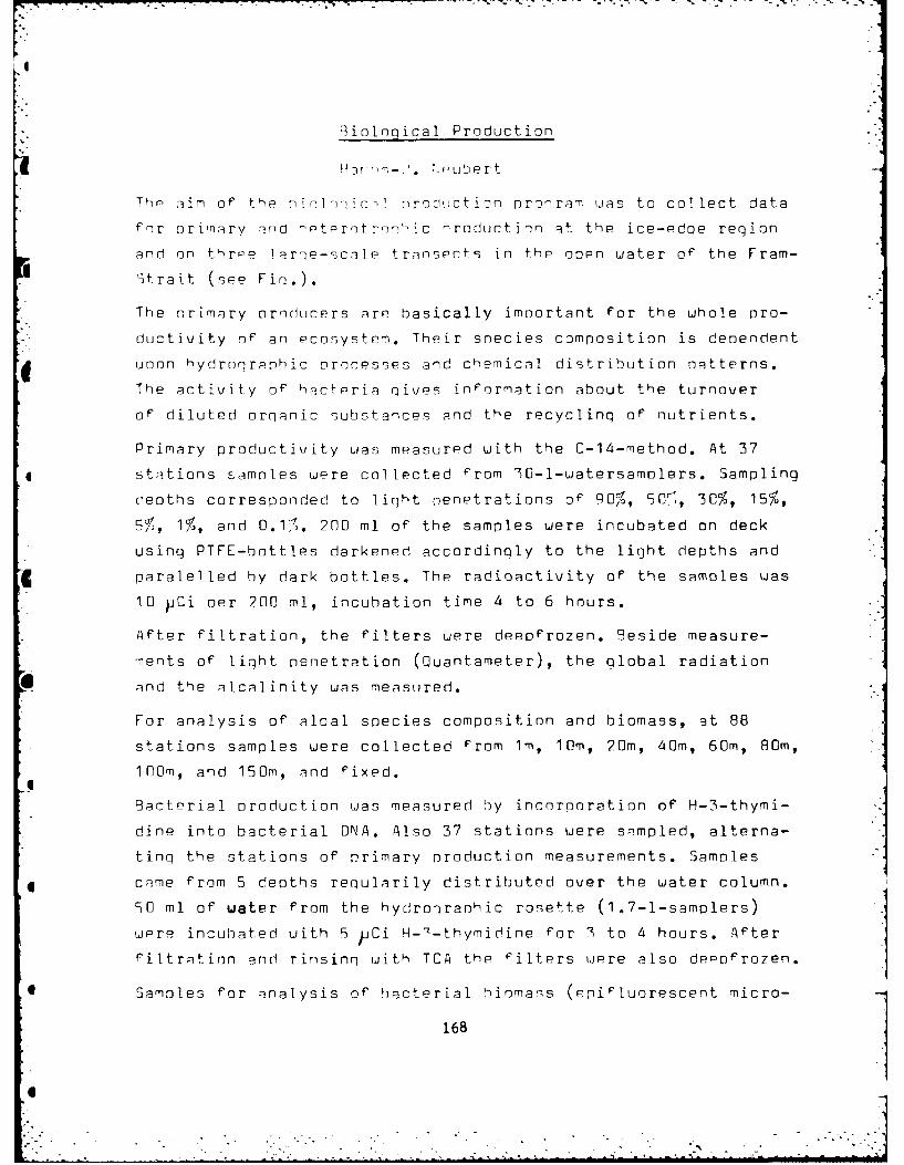
.4

Riolngical Production

Thr aim of thp hjql-irlic7 nrcl,iJction praqram was to collect data

for [orimary 3roc! PtPrtrnnOic nroduction at the ice-edqe region

and on thrpe laroe-scale transects in the open water of the Fram-

Strait (see Fin.).

The nrimary producers are basically important for the whole pro-

ductivity of an ecosystem. Their snecies composition is dependent

unon hydronranhic orocesses and chemical distribution natterns.

The activity of bactpria gives information about the turnover

of diluted organic substances and the recycling of nutrients.

Primary productivity was measured with the C-14-method. At 37

stations samples were collected from 30-1-watersamplers. Sampling

depths corresponded to light nenetrations oF 90%, 50r, 30%, 15%,

5%, 1%, and 0.1'1. 200 ml of the samples were incubated on deck

using PTFE-bottles darkened accordingly to the light depths and

paralelled by dark bottles. The radioactivity of the samples was

10 pCi oer 200 ml, incubation time 4 to 6 hours.

After filtration, the filters were deenfrozen. Beside measure-

ments of light penetration (Quantameter), the global radiation

and the alcalinity was measured.

For analysis of aloal species composition and biomass, at 88

stations samples were collected from Im, 10m, 20m, 40m, 60m, 80m,

lo0m, and 150m, and fixed.

9acterial production was measured by incorporation of H-3-thymi-

dine into bacterial DNA. Also 37 stations were sampled, alterna-

ting the stations of primary production measurements. Samples

4 came from 5 depths renularily distributed over the water column.

90 ml of water from the hydronranhic rosette (1.7-1-samplers)

wpre incubated with 9 PCi H- 7-thymidine for 3 to 4 hours. After

filtration and rinsing with TCA the Filters were also depfrozen.

4 Samples for analysis of bacterial biomass (epifluorescent micro-

168 III

- ... i.

lr",)y w re t,-'en from 1iF (Ueth at H.E3 sta t icns.

A~t F-, at ion no. 15 7,nmnr I-pnFr qupnrh corr-ct ions upre tr -n, -. t

st~itjcn no. '?r)F the jnF'li-unce of OifC-rent bottlp rat-rials

(m-I , P', PTFE) on thep - rrltct ion w,-9 tested.

4 Natural Tritium Content

Hanns-J. Neubert

* ~ At station no. 333 (see Fiq.) a hole of' >7000 m was f'ound. To qet

inf'ormation about the ane of' the uater in that hole and the turn-

ovier of' the deeoater, samoles "rom 19 deoths wpre taken f'or

analysis of the natural concentration of' tritium (-)

169

W4 00 E 0

80NLI l 'i, £10 El 80ONN80.* NS80

78ON LJ;bo* 78 *N

W 00 E 100

170

The Phytoplankton and the Primary Production

*\. E.M. Baumann, RWTH Aachen, Bio I, Abt.f.Syst.u. Geobot.

1. Distribution of Phytoplankton

The aim of these investigations was the vertical and horizontal

distribution of the phytoplankton. Samples were taken at every

biological station (see tab.) from the surface down to a light

depth of 16 %. The light depths were determined by secchi disk

and quantameter.

2. Primary Production

The primary production was estimated on the basis of 14C- assi-

milation for different light depths (7o%, 5o%, 3o%, 16%) with

the help of a recently developed incubator. The diurnal changes

of the light intensities were measured by a photocell installed

on a retractable girder above the crow's nest and automatically

simulated in the incubator with fluorescent tubes of a similar

spektrum as the solar light. The light depths were simulated

with different filters, the temperature was adjusted with the

aid of two aggregates at every station where measurements were

undertaken (see tab.). The production measurements were carried

out in untreated samples and in 2o um and Io um fractionated

samples to get an idea on the contribution of the nannoplankton

to the primary production.

3. Isolation and Cultivation of Phytoplankton

The dominant diatom species were isolated from the phytoplankton

and cultivated in filtered seawater to which nutrients had been

added. The following species were isolated: Thalassiosira gravida,

T. nordenski6ldii, Chaetoceros decipiens, C. socialis, C. borealis.

Amphiprora hyperborea, Bacteriosira fragilis, Lauderia borealis.

171

* and some Fragillaria- and Coscinodiscus species. In addition,

primary production was measured on these under natural conditions

in the incubator to determine the contribution of these respec-

tive species to the total sum of primary production. The enlistcd

diatom species were taken home for additional eco-physiological

experiments.

g4. Further Primary Production Measurements

During the 2nd minidrift, some "in situ"- incubations could be

undertaken. The incubation bottles were fastened to a rope accor-

If ding to the appropriate light depths and were allowed to swim

behind the stern of the ship in the open water where ice floes

did not disturb the incubation. Furthermore, isolated algae

material was incubated below the ice through a hole drilled by

* the glaciologists at station 299 to get an idea about the pro-

ductivity of the algae under these light defficient conditions

and to test the practicability of such measurements.

a 5. Light Measurements

"- Vertical profiles of the light conditions in the natural water

column were measured from the ship and from the rubber boat in

@, open water and between ice floes in pack ice. The diurnal changes

of the daylight were measured continously.

I*1

0

172

Stat ion No. Watertemp. Secchidepth Depths of the incubated samples°C m mn

174 o,6 17 o,6,11.17

178 o,6 17 o,6,11,17

182 -1,2 2o o,5,11,2o

183 o.3 12 3,5,12,3o

188 1. 3 6 2,3.6,2o

19o 2.2 11 -

198 -o8 19 5,8,21.52

2ol 1, 5 9 4, 7,1o

2o3 2,6 8 4.6,9

. i n dI'i f t -0,5 11 3,5,7.11

-o.5 11 5,8,12,4o

223 -1.o 16 o, 9,1828

221 o.3 lo 4,11

225 -o,6 8 5,6

226 -1.4 18 5,7.11,18,28.43

229 -1,4 21 5,8.14,21

2:32 -2,5 2o 8,14,2o,loo

239 -1,6 25 lo,18.29.35,75

245 -o,5 lo 5,8,12.2o,3o

25:3 -o.8 25 7,16.25, 39,6o, 8926o o.3 11 5,8.12.19.3o,45

264 0.0 11 5,8.12,2o,3o,45

271 -n n 18 13,2o

272 -1.9 26 o,18.29

273 -1,7 15 o,6,11,17

275 3,2 11 4,7.11

277 o.6 15 o.5.9,15

28o -1.o 14 o,5,9,14

283 -1.5 22 o.9.16.25

287 1.3 1o 4,6.1o

28s 4.o 6 o, 5.7

291 1.5 7 o,3.5,8

294 1 5 7 o 3,5.8

296 -1.4 8 o.8

296 (2) 0.0 8 1, ..10

297 -1,8 8 o,2.8

298 -o,4 7 1.3,5,7

299 0,0 lo 1,4,7.1o

300 -1,7 12 2.5,8,12

3o2 -1.5 14 3.6,lo,14

3o4 -o.9 12 2,4.8.12

Tab. Primary Production: On these stations primary produlction measurements were undertaken

dwl, i i l the ,IZEX - cruise 1984

173

Phytoplankton Ecology and Zooplankton Grazing

J. Lenz, K.-G. Barthel, R. Gradinger, I.f.M. Kiel, Germany

Within the framework of the joint biological program on board the RV

'Polarstern' we concentrated our sampling program on phytoplankton,

particulate matter and microzooplankton in the euphotic zone and below,

down to 200 m. Samples were preserved for the analysis of species com-

position dnd after filtration deep-frozen for subsequent measurement of

seston, particulate carbon and nitrogen and chlorophyll a. At each

full-program station, dominant copopod species were sorted out and graz-

ing experiments performed under natural feeding conditions. An addition-

al program was the measurement of photosynthetic active radiation es-

sential for phytoplankton growth in leads and under ice-floes. Altoge-

ther, over 40 stations were occupied. Preliminary results showed that

planktoi, abundance and species composition are largely governed by the

hydrographic structure of the water masses and the extent of ice cover.

Three main areas differing in seasonal development of phyto- and zoo-

£ plankton were encountered on the east-west transect through the Fram

Strait. The first is the Ice Edge Zone strongly influenced by North

Atlantic waters with high phytoplankton standing stocks and corre-

spondingly low water transparency. A characteristic feature was a sub-

4surface maximum of algae below the low-saline ice-melt water. Species

composition pointed to a post-spring bloom of phytoplankton. This zone

was also characterized by high concentrations of actively grazing cope-

pod populations. Very clear waters sparse in plankton constitute the

E second region in the center of the pack-ice zone. The few copepods pre-

sent were still in their hibernating resting stage and had not yet

started grazing. The third area are the large polynias at the East

Greenland shelf edge. Here the phytoplankton spring bloom was approach-

ing its peak with actively feeding meroplanktic larvae and copepods. A

much more detailed picture will be obtained after completion of the

time-consuming analysis of the samples, which will take about a year.

174

Distribution of nutrients and organic substances

C. Kattner

According to the station grid of the CTD-measurements more

than 2200 samples were taken for chemical analysis. At every

station 12 or 24 samples were taken; major sampling depths!were 500 m and until bottom. Nutrients - nitrate, nitrite,

phosphate, silicate, and ammonia - were measured immediatelyfrom unfiltered samples by a Technicon AutoAnalyzer. Addi-

tionally all samples were filtered through glass fibre filters

and preserved by mercury chloride for analysis of organic

substances. These measurements will be performed in the

institute in Hamburg.

In the upper water layer good correlations seem to exist be-

tween the nutrients and the biological activity. In the area

of the ice edge the nutrient concentrations were rather low,

which indicates a high productivity before or during the

experiment. Especially nitrate was nearly exhausted in the

euphotic zone and seems to be the limiting factor of the

phytoplankton growth. The concentrations of the other

nutrients were slightly higher, increasing all towards the

ice covered regions. The concentrations of nitrate, silicate

and phosphate increased with depths reaching maximum values

near the bottom. Ammonia and nitrite, resulting from de-

composition processes and release of zooplankton, showed

* highest concentrations at 30 to 80 m in the ice edge region.

That seems to be in connection with zooplankton activity.

The distribution of nutrients also permits a characterization

of water masses. During the large scale survey the transport

of water out of the Arctic Ocean could be identified by

high concentration of nutrients. More than 20 umoles dm of-3

silicate and 1.5 Pmoles dm - 3 of phosphate were observed in a

layer between 50 and 100 m depth. For example, the silicate

175

k-3

concentration decreased from about 21 umoles dm at 80 m

to 6 umoles dm - 3 below 100 m depth. Also the deep water

I nutrient distribution will help to identify and quantify

water mass exchange and transport.

Additionally to the seawater analyses nutrients were

I measured in about 400 samples of melted sea ice. In co-

operation with the group of CRREL, investigating sea ice

properties, ice cores of 14 multi and first year ice floes

were studied. Each core was analyzed at nominal 10 or 20 cm

|E intervals. Silicate showed higher concentrations than the

other nutrients with clear maxima especially in the multi

year ice cores. In general the nutrient concentrations of the

ice floes were lower than those in the sea water.

1

a

I

- 176

I'

FILMED

2-85

* DTIC