Embed Size (px)
Citation preview

NBER WORKING PAPER SERIES
R&D INVESTMENT, EXPORTING, AND PRODUCTIVITY DYNAMICS
Bee Yan AwMark J. Roberts
Daniel Yi Xu
Working Paper 14670http://www.nber.org/papers/w14670
NATIONAL BUREAU OF ECONOMIC RESEARCH1050 Massachusetts Avenue
Cambridge, MA 02138January 2009
We thank Jan De Loecker, Ulrich Doraszelski, Marc Melitz, Ariel Pakes, Nina Pavnick, and Jim Tyboutfor helpful discussions and comments. We are grateful to Yi Lee for helping us to acquire and understandthe data. All remaining errors are ours. The views expressed herein are those of the author(s) and donot necessarily reflect the views of the National Bureau of Economic Research.
NBER working papers are circulated for discussion and comment purposes. They have not been peer-reviewed or been subject to the review by the NBER Board of Directors that accompanies officialNBER publications.
© 2009 by Bee Yan Aw, Mark J. Roberts, and Daniel Yi Xu. All rights reserved. Short sections oftext, not to exceed two paragraphs, may be quoted without explicit permission provided that full credit,including © notice, is given to the source.

R&D Investment, Exporting, and Productivity DynamicsBee Yan Aw, Mark J. Roberts, and Daniel Yi XuNBER Working Paper No. 14670January 2009, Revised October 2010JEL No. F14,O31,O33
ABSTRACT
A positive correlation between productivity and export market participation has been well documentedin producer micro data. Recent empirical studies and theoretical analyses have emphasized that thismay reflect the producer's other investment activities, particularly investments in R&D or new technology,that both raise productivity and increase the payoff to exporting. In this paper we develop a dynamicstructural model of a producer's decision to invest in R&D and participate in the export market. Theinvestment decisions depend on the expected future profitability and the fixed and sunk costs incurredwith each activity. We estimate the model using plant-level data from the Taiwanese electronics industryand find a complex set of interactions between R&D, exporting, and productivity. The self- selectionof high productivity plants is the dominant channel driving participation in the export market and R&Dinvestment. Both R&D and exporting have a positive direct effect on the plant's future productivitywhich reinforces the selection effect. When modeled as discrete decisions, the productivity effect ofR&D is larger, but, because of its higher cost, is undertaken by fewer plants than exporting. The impactof each activity on the net returns to the other are quantitatively unimportant. In model simulations,the endogenous choice of R&D and exporting generates average productivity that is 22.0 percent higherafter 10 years than an environment where productivity evolution is not affected by plant investments.
Bee Yan AwDepartment of EconomicsThe Pennsylvania State UniversityUniversity Park, PA [email protected]
Mark J. RobertsDepartment of Economics513 Kern Graduate BuildingPennsylvania State UniversityUniversity Park, PA 16802and [email protected]
Daniel Yi XuDepartment of EconomicsNew York University19 West Fourth Street, Sixth FloorNew York, NY 10012and [email protected]

R&D Investment, Exporting, and Productivity Dynamics
By BEE YAN AW, MARK J. ROBERTS, AND DANIEL YI XU�
This paper estimates a dynamic structural model of a producer's decisionto invest in R&D and export, allowing both choices to endogenously affect thefuture path of productivity. Using plant-level data for the Taiwanese electronicsindustry, both activities are found to have a positive effect on the plant's futureproductivity. This in turn drives more plants to self-select into both activities,contributing to further productivity gains. Simulations of an expansion of theexport market are shown to increase both exporting and R&D investment andgenerate a gradual within-plant productivity improvement.JEL: F14, O31, O33Keywords: Export, R&D investment, Productivity Growth, Taiwan ElectronicsIndustry
A large empirical literature using �rm and plant-level data documents that, on average, export-ing producers are more productive than nonexporters. A general �nding is that this re�ects theself-selection of more productive �rms into the export market but, in some cases, may also re�ecta direct effect of exporting on future productivity gains.1 A further possibility is that there is aspurious component to the correlation re�ecting the fact that some �rms undertake investmentsthat lead to both higher productivity and a higher propensity to export.Recently, several authors have begun to measure the potential role of the �rms' own invest-
ments in R&D or technology adoption as a potentially important component of the productivity-export link. Andrew B. Bernard and J. Bradford Jensen (1997), Mary Hallward-Driemeier,Giuseppe Iarossi, and Kenneth L. Sokoloff (2002), John R. Baldwin and Wulong Gu (2004), BeeYan Aw, Mark J. Roberts, and Tor Winston (2007), Paula Bustos (forthcoming), Alla Lileevaand Daniel Tre�er (forthcoming), Leonardo Iacovone and Beata S. Javorcik (2007), Bee Yan Aw,Mark J. Roberts, and Daniel Yi Xu (2008) and Jo�e P. Damijan, �Crt Kostevc, and Sa�o Polanec(2008) �nd evidence from micro data sets that exporting is also correlated with �rm investmentin R&D or adoption of new technology that can also affect productivity. Complementing thisevidence, Chiara Criscuolo, Jonathan Haskel, and Matthew Slaughter (2005) analyze survey datacollected for E.U. countries and �nd that �rms that operate globally devote more resources to as-similating knowledge from abroad and generate more innovations and productivity improvement.A key implication of these studies is that the technology and export decisions are interdependentand both channels may endogenously affect the �rm's future productivity.The effects of a trade liberalization that lowers trade costs or expands export markets will de-
pend crucially on the micro-level relationship between productivity, exporting, and R&D or tech-nology investment. Two recent theoretical papers, Andrew Atkeson and Ariel Burstein (forth-coming) and James A. Constantini and Marc J. Melitz (2008), have formalized how trade liberal-izations can increase the rate of return to a �rm's R&D or investment in new technology and thus
� Aw: The Pennsylvania State University, Department of Economics, 501 Kern Building, University Park, PA 16870,(e-mail: [email protected]). Roberts: The Pennsylvania State University, Department of Economics, 513 Kern Building,University Park, PA 16870 and National Bureau of Econmic Research, (e-mail: [email protected]). Xu: New YorkUniversity, Department of Economics, 19 West Fourth Street, Sixth Floor, New York, NY 10012 and National Bureauof Economic Research, (e-mail: [email protected]). We thank Jan De Loecker, Ulrich Doraszelski, Jonathan Eaton,José Carlos Fariñas, Oleg Itskhoki, Marc Melitz, Ariel Pakes, Nina Pavnick, Jim Tybout and two anonymous referees forhelpful discussions and comments. We are grateful to Yi Lee for helping us to acquire and understand the data. Allremaining errors are ours.
1See Greenaway and Kneller (2007) for a recent survey of the micro econometric evidence on this topic.
1

2 THE AMERICAN ECONOMIC REVIEW MONTH YEAR
lead to future endogenous productivity gains. Both papers share several common features. First,productivity is the underlying state variable that distinguishes heterogeneous producers. Second,productivity evolution is endogenous, affected by the �rm's innovation decisions, and contains astochastic component. Third, while they differ in the speci�c structure of costs and information,they each identify pathways through which export market size affects the �rm's choice to exportor invest in new technology. Quantifying these pathways is key to understanding the long-runimpacts of trade liberalization.In this paper we develop and estimate a dynamic, structural model of exporting and R&D
investment using data for Taiwanese manufacturing plants in the electronics products industry forthe period 2000-2004. We use the model to quantify the linkages between the export decision,R&D investment, and endogenous productivity growth and then simulate the long-run impactsof an export demand expansion on these variables. This provides a methodology for studyingthe effects of trade liberalization on productivity growth without data from a natural experiment.As part of our model we estimate the dynamic decision rules for the plant's optimal choice ofR&D and exporting where these rules depend on the expected future pro�ts and the current �xedor sunk costs of each activity. We quantify three pathways linking exporting, R&D investment,and productivity. First, the return to each investment increases with the producer's underlyingproductivity which leads high-productivity producers to self-select into both investment activities.Second, each investment directly affects future productivity which acts to reinforce the selectioneffect. Third, as emphasized in the recent theoretical models, policy changes that alter the futurereturn to one activity, such as a reduction in trade costs or an R&D subsidy, affect the probabilityof both activities.Our empirical results reveal a rich set of productivity determinants. Productivity evolution
is endogenous, being impacted positively by both R&D investment and exporting and, whenmodeled as discrete activities, the impact of R&D is larger. There are signi�cant entry costsfor both activities, which introduces a second source of intertemporal linkages in the decisions,and the costs of undertaking R&D activities are larger than the costs of exporting. The self-selection of high productivity plants is the dominant channel driving export market participationand R&D investment and this is reinforced by the effect of each investment on future productivity.Holding expected export market demand constant, whether or not a �rm invested in R&D inthe past has very little direct impact on the net returns to exporting or the probability the �rmexports. Similarly, past export experience has very little direct impact on the return to R&D orthe probability of undertaking R&D.Using the model we conduct counterfactual exercises to quantify the effect of a permanent
reduction in trade costs that increases export demand on plant exporting, R&D, and productivitychange. Bustos (forthcoming) and Lileeva and Tre�er (forthcoming) have studied periods oftrade liberalization in Argentina and Canada and found evidence that reductions in tariffs facedby exporting �rms lead to increases in exporting, innovative activities by the �rm, or productivity.We �nd that an expansion in export market size would increase the export and R&D participationrates by 10.2 and 4.7 percentage points, respectively, after 15 years. This would lead to anincrease in mean plant productivity of 5.3 percent. This re�ects the cumulative effect of increasedexporting and R&D on productivity and the effect of these productivity gains on the self-selectionof plants into these activities. We isolate the individual roles of R&D and exporting by comparingour counterfactual results with those generated by more restrictive productivity processes and �ndthat, in the environment with endogenous plant productivity, the expansion of the export marketleads to an increase in mean productivity that is twice as large as the increase that would occurunder more restrictive environments. The combination of larger export markets and the plant'sability to invest and endogenously affect its future productivity contributes to larger productivitygains.The next section of this paper develops the theoretical model of the �rm's dynamic decision to
invest in R&D and exporting. The third section develops a two-stage estimation method for the

VOL. VOL NO. ISSUE R&D, EXPORTING, PRODUCTIVITY DYNAMICS 3
model. The �rst stage estimates the underlying process for producer productivity and the secondstage uses this to estimate the dynamic decision rules for R&D and export market participation.The fourth section provides a brief discussion of the data source. The �fth section summarizesthe parameter estimates, measures the costs and marginal returns to R&D investment and exportmarket participation, and conducts the counterfactual exercise to quantify the productivity effectsof an expansion of export demand.
I. A Structural Model of Exporting and R&D
The theoretical model developed in this section is similar in several ways to the models ofexporting developed by Mark J. Roberts and James R. Tybout (1997), Sofronis K. Clerides, SaulLach, and James R. Tybout (1998), Marc J. Melitz (2003), and Sanghamitra Das, Mark J. Roberts,and James R. Tybout (2007) and the models of exporting and investment by Atkeson and Burstein(forthcoming) and Constantini and Melitz (2008). We abstract from the decision to enter or exitproduction and instead focus on the investment decisions and process of productivity evolution.Firms are recognized to be heterogeneous in their productivity and the export demand curve theyface. Together these determine each �rm's incentive to invest in R&D and to export. In turn,these investments have feedback effects that can alter the path of future productivity for the �rm.We divide the �rm's decision making into a static component, where the �rm's productivity de-termines its short-run pro�ts from exporting, and a dynamic component where they make optimalR&D and export-market participation decisions.
A. Static Decisions
We begin with a model of the �rm's revenue in the domestic and export markets. Firm i'sshort-run marginal cost function is written as:
(1) lnci t D lnc.ki t ; wt /� !i t D �0 C �k ln ki t C �w lnwt � !i t
where ki t is �rm capital stock, wt is a vector of variable input prices common to all �rms, and !i tis �rm productivity.2 Several features of the speci�cation are important. The �rm is assumedto produce a single output which can be sold in both domestic and export markets and marginalcost is identical across the two markets for a �rm. There are two sources of short-run cost het-erogeneity, capital stocks that are observable in the data and �rm productivity that is observableto the �rm but not observable in our data. Marginal cost does not vary with the �rm's outputlevel which implies that demand shocks in one market do not affect the static output decision inthe other market and allows us to model revenue and pro�ts in each market independently of theoutput level in the other market.3Both the domestic and export markets are assumed to be monopolistically competitive and
segmented from each other. This rules out strategic interaction among �rms in each market butdoes allow �rms to charge markups that differ across markets. The demand curves faced by �rmi in the domestic and export markets are assumed to have the Dixit-Stiglitz form. In the domesticmarket it is:
(2) qDit D QDt .p
Dit =P
Dt /
�D DI DtPDt
.pDitPDt
/�D D 8Dt .pDit /�D
2Other �rm-level cost shifters can be included in the empirical speci�cation. In this version we will focus on theheterogeneity that arises from differences in size, as measured by capital stocks, and productivity.
3The domestic market will play an important role in modeling the dynamic decision to invest in R&D developed later.

4 THE AMERICAN ECONOMIC REVIEW MONTH YEAR
where QDt and PDt are the industry aggregate output and price index, I Dt is total market size, and�D is the constant elasticity of demand. The �rm's demand depends on the industry aggregates,represented by 8Dt ; its price pDit , and the constant demand elasticity.
A similar structure is assumed in the export market except that each �rm's demand also de-pends on a �rm-speci�c demand shifter zi t . The demand curve �rm i faces in the export marketis:
(3) qXit DI XtP Xt.pXitP Xt/�X exp.zi t / D 8Xt .p
Xit /�X exp.zi t /
where 8Xt represents the aggregate export market size and price, pXit is the �rm's export price,�X is a common demand elasticity and zi t is a �rm-speci�c demand shock. By including thislast term we incorporate an exogenous source of �rm-level variation which will allow a �rm'srelative demands in the domestic and export markets to vary across �rms and over time. The�rm is assumed to observe zi t when making its export decision, but it is not observable in ourdata.
Given its demand and marginal cost curves, �rm i chooses the price in each market to maximizethe sum of domestic and export pro�ts. The �rst-order condition for the domestic market pricepDit implies that the log of domestic market revenue r
Dit is:
(4) ln rDit D .�D C 1/ ln.�D
�D C 1/C ln8Dt C .�D C 1/.�0 C �k ln ki t C �w lnwt � !i t /
Speci�cally, the �rm's revenue depends on the aggregate market conditions and the �rm-speci�cproductivity and capital stock. Similarly, if the �rm chooses to export, export market revenue is:
(5) ln r Xit D .�X C 1/ ln.�X
�X C 1/C ln8Xt C .�X C 1/.�0 C �k ln ki t C �w lnwt � !i t /C zi t
depending on the aggregate export market conditions, �rm productivity, capital stock, and theexport market demand shock. In the context of this model, these two equations show that the�rm's domestic revenue will provide information on its marginal cost, in particular the produc-tivity level !i t . The export market revenue will also provide information on the export demandshocks, but only for �rms that are observed to export. In the empirical model developed below wewill estimate the revenue functions and can interpret the two sources of unobserved heterogeneity!i t and zi t more generally. The �rst term !i t will capture any source of �rm-level heterogeneitythat affects the �rm's revenue in both markets. While we will refer to this as productivity, itcould include characteristics of the product, such as its quality, that would affect the demand forthe �rm's product, as well as its cost, in both markets. The zi t term will capture all sources ofrevenue heterogeneity, arising from either the cost or demand side, that are unique to the exportmarket. We will refer to zi t as the �rm's export market shock.
Given these functional form assumptions for demand and marginal cost, there is a simple linkbetween �rm revenue and pro�t in each market. The �rm's pro�t in the domestic market is:
(6) �Dit D �.1�D/rDit .8
Dt ; ki t ; !i t /
where revenue is given above. Similarly, if the �rm chooses to export, the pro�ts they will earn
VOL. VOL NO. ISSUE R&D, EXPORTING, PRODUCTIVITY DYNAMICS 5
are linked to export market revenue as:
(7) � Xit D �.1�X/r Xit .8
Xt ; ki t ; !i t ; zi t /
These equations allow us to measure �rm pro�ts from observable data on revenue in each market.These short-run pro�ts will be important determinants of the �rm's decision to export and toinvest in R&D in the dynamic model developed in the next two sections.
B. Transition of the State Variables
In order to model the �rm's dynamic optimization problem for exporting and R&D we beginwith a description of the evolution of the process for �rm productivity !i t and the other statevariables ln8Dt , ln8Xt , zi t , and ki t . We assume that productivity evolves over time as a Markovprocess that depends on the �rm's investments in R&D, its participation in the export market, anda random shock:
!i t D g.!i t�1; di t�1; ei t�1/C � i t(8)D �0 C �1!i t�1 C �2.!i t�1/
2 C �3.!i t�1/3 C �4di t�1 C �5ei t�1 C
�6di t�1ei t�1 C � i t
di t�1 and ei t�1 are, respectively, the �rm's R&D and export market participation in the previousperiod. The inclusion of di t�1 recognizes that the �rmmay affect the evolution of its productivityby investing in R&D. The inclusion of ei t�1 allows for the possibility of learning-by-exporting,that participation in the export market is a source of knowledge or expertise that can improve fu-ture productivity. The stochastic nature of productivity improvement is captured by � i t which istreated as an i id shock with zero mean and variance � 2� .
4 This stochastic component representsthe role that randomness plays in the evolution of a �rm's productivity. It is the innovation in theproductivity process between t � 1 and t that is not anticipated by the �rm and by construction isnot correlated with !i t�1; di t�1; and ei t�1. This speci�cation also recognizes that the stochasticshocks to productivity in any year t will carry forward into productivity in future years. The sec-ond line of the equation gives the assumed functional form for this relationship: a cubic functionof lagged productivity and a full set of interactions between lagged exporting and R&D.We model the past R&D and export choice, di t�1; and ei t�1, as discrete 0/1 variables which
implies that any �rm that undertakes R&D or exporting has the same expected increment to itsproductivity, as described by the parameters �4; �5;and �6 (the realizations will differ becauseof the stochastic component � i t ). This is consistent with the evidence reported by Aw, Roberts,and Winston (2007) who estimate a reduced-form model consistent with the structural modelwe develop here. They �nd that productivity evolution for Taiwanese electronics producers isaffected by the discrete export and R&D variables. They also �nd that �rm productivity is asigni�cant determinant of the discrete decision to undertake each of these activities, but �nd littleevidence that productivity is correlated with the level of export market sales for �rms that choosethese investments.
4This is a generalization of the productivity process used by G. Steven Olley and Ariel Pakes (1996) in their workon productivity evolution in the U.S. telecommunications industry. They modeled productivity as an exogenous Markovprocess !i t D g.!i t�1/ C � i t : Ulrich Doraszelski and Jordi Jaumandreu (2007) have endogenized productivity byallowing it to depend on the �rm's choice of R&D. They model productivity as !i t D g.!i t�1; di t�1/ C � i t wheredi t�1 is the �rm's past R&D expenditure. They also show how their speci�cation generalizes the "knowledge capital"model of productivity developed by Zvi Griliches (1979, 1998).
6 THE AMERICAN ECONOMIC REVIEW MONTH YEAR
The �rm's export demand shock will be modeled as a �rst-order Markov process:
(9) zi t D �zzi t�1 C �i t ; �i t � N .0; � 2�/:
If a source of �rm-level heterogeneity like z was not included in this model, there would be aperfect cross-section correlation between domestic and export revenue. In our application it isimportant to allow persistence in the evolution of z because it is going to capture factors like thenature of the �rm's product, the set of countries they export to, and any long-term contractual orreputation effects that lead to persistence in the demand for its exports over time.5In modeling the dynamic decisions to export and invest in R&D, the �rm's capital stock, ki ;
will be treated as �xed over time. We recognize the differences in capital stocks across �rms butdo not attempt to model the �rm's investment in capital. Given the relatively short time seriesin our data, virtually all the variation in capital stocks is across �rms and there is nothing to begained in our empirical application by the additional complication of modeling the �rm's capitalstock as an endogenous state variable. Finally, the aggregate state variables ln8Dt and ln8Xt aretreated as exogenous �rst-order Markov processes that will be controlled for using time dummiesin the empirical model.
C. Dynamic Decisions - R&D and Exporting
In this section we develop the �rm's dynamic decision to export and invest in R&D. A �rmentering the export market will incur a nonrecoverable sunk cost and this implies that the �rm'spast export status is a state variable in the �rm's export decision. This is the basis for the dynamicmodels of export participation developed by Roberts and Tybout (1997) and Das, Roberts, andTybout (2007). We will also incorporate a sunk startup cost for the �rm when it begins investingin R&D and this will make the �rm's past R&D status a state variable in the investment choices.This is similar to Daniel Yi Xu (2008) who estimates a dynamic model of �rm R&D choice whereR&D expenditures affect the future productivity of the �rm. Finally, in our model there is oneadditional intertemporal linkage: productivity is endogenous meaning the �rm's export and R&Dchoices can affect its future productivity as shown in equation 8.While the static pro�ts, equations 6 and 7, earned by the �rm are one important component of
its decisions, these will also depend on the combination of markets it participates in and the �xedand sunk costs it must incur. It is necessary to make explicit assumptions about the timing of the�rm's decision to export and undertake R&D. We assume that the �rm �rst observes values of the�xed and sunk costs of exporting, Fit and
Sit ; and makes its discrete decision to export in year
t . Following this, it observes a �xed and sunk cost of investment, Ii t and Dit ; and makes the
discrete decision to undertake R&D.6 These costs are the expenditures that the �rm must maketo realize the productivity gains that are given by equation 8. These expenditures will differacross �rms because of differences in technological opportunities and expertise and we assumethe �rm observes its required expenditure before it makes its discrete decision to undertake R&D
5This formulation does not imply that the �rm's R&D cannot affect its pro�tability in the export market. We justassume that whatever role R&D plays it works through ! and affects the �rm's revenue and pro�ts in both the domesticand export market. In our data, the R&D variable measures the �rm's investments to develop and introduce new productsand to improve its production processes. This variable is best incorporated in our model by allowing it to affect bothmarkets. If separate data were available on R&D expenditures to develop new products and expenditures to improveproduction processes then some other speci�cations could be developed. For example, it would be possible to allow theprocess R&D variable to affect both markets through ! while the new product expenditures acted to shift export demandthrough z.
6An alternative assumption is that the �rm simultaneously chooses d and e. This will lead to a multinomial modelof the four possible combinations of exporting and R&D investment. In the empirical application, it is more dif�cult tocalculate the probability of each outcome in this environment.

VOL. VOL NO. ISSUE R&D, EXPORTING, PRODUCTIVITY DYNAMICS 7
or export. Since we do not know the underlying technological opportunities for each �rm wemodel these four expenditures as i id draws from a known joint distribution G : One goal of theempirical model is to estimate parameters that characterize the cost distribution.The state vector for �rm i in year t is si t D .!i t ; zi t ; ki ;8t ; ei t�1;di t�1/ and the �rm's value
function in year t; before it observes its �xed and sunk costs, can be written as:
(10) Vi t .si t / DZ.�Dit C maxei t
f.� Xit � ei t�1 Fit � .1� ei t�1/
Sit /C V
Eit .si t /; V
Dit .si t /g/dG
where ei t�1 is a discrete 0/1 variable identifying the �rm's export status in t � 1. If the �rmexported in t � 1 it pays the �xed cost Fit when exporting in period t , otherwise it pays the sunkentry cost Sit to participate. V
E is the value of an exporting �rm after it makes its optimal R&Ddecision and, similarly, V Dit is the value of a non-exporting �rm after it makes its optimal R&Ddecision. This equation shows that the �rm chooses to export in year t when the current plusexpected gain in future export pro�t exceeds the relevant �xed or sunk cost. In this equation thevalue of investing in R&D is subsumed in V Dit and V
Eit . Speci�cally,
V Eit .si t / D
Zmaxdi tf�EtVi tC1.si tC1jei t D 1; di t D 1/� di t�1 Ii t � .1� di t�1/
Dit ;(11)
�EtVi tC1.si tC1jei t D 1; di t D 0/gdG
The �rst term shows that if the �rm chooses to undertake R&D .di t D 1/ then it pays a currentcost that depends on its prior R&D choice. If it invested in R&D in t � 1 then it pays the�xed investment cost Ii t otherwise it pays the sunk startup cost
Dit : It has an expected future
return which depends on how R&D affects future productivity. If they do not choose to invest.di t D 0/ they have a different future productivity path. The larger the impact of R&D on futureproductivity, the larger the difference between the expected returns of doing R&D versus notdoing R&D and thus the more likely the �rm is to invest in R&D. Similarly, the value of R&D toa non-exporting �rm is:
V Dit .si t / D
Zmaxdi tf�EtVi tC1.si tC1jei t D 0; di t D 1/� di t�1 Ii t � .1� di t�1/
Dit ;(12)
�EtVi tC1.si tC1jei t D 0; di t D 0/gdG
where the �rm faces the same tradeoff, but now the future productivity paths will be those for anon-exporter. Finally, to be speci�c, the expected future value conditional on different choicesfor ei t and di t is:
(13) EtVi tC1.si tC1jei t ; di t / DZ80
Zz0
Z!0
Vi tC1.s0/dF.!0j!i t ; ei t ; di t /dF.z0jzi t /dG.80j8t /
In this equation the evolution of productivity dF.!0j!i t ; ei t ; di t / is conditional on both ei t anddi t because of the assumption in equation 8.In this framework, the net bene�ts of both exporting and R&D investment are increasing in
current productivity. This leads to the usual selection effect where high productivity �rms aremore likely to export and invest in R&D. By making future productivity endogenous, this modelrecognizes that current choices lead to improvements in future productivity and thus more �rms
8 THE AMERICAN ECONOMIC REVIEW MONTH YEAR
will self-select into, or remain in, exporting and R&D investment in the future.When we have two choice variables for the �rm, there are new forces in addition to the selec-
tion effect which make the decisions interdependent. First, whether or not the �rm chooses toexport in year t affects the return to investing in R&D. For any state vector, we can de�ne themarginal bene�t of doing R&D from equations 11 and 12 as the difference in the expected futurereturns between choosing and not choosing R&D:
(14) MBRi t .si t jei t / D EtVi tC1.si tC1jei t ; di t D 1/� EtVi tC1.si tC1jei t ; di t D 0/:
This will depend on the impact of R&D on future productivity but also on the �rm's export choiceei t because of the effect of the sunk cost of exporting and the direct effect of exporting on futureproductivity through equation 8. In the special case where the sunk cost of exporting Sit D 0 andexporting does not affect the evolution of productivity (�5 D �6 D 0 in equation 8), exportingbecomes a static decision and MBRi t will not be a function of ei t implying that an exporter anda non-exporter will have the same valuation of R&D investment.7In general, MBRi t will differ for exporters and nonexporters and the sign and magnitude of
the difference will depend on the combined effect of the sunk cost of exporting and the sign of theinteraction effect between R&D and exporting on productivity, which is given by the coef�cient�6 in equation 8. De�ne the difference in the future bene�t of R&D between exporters andnonexporters as 1MBRi t .si t / D MBRi t .si t jei t D 1/ � MBRi t .si t jei t D 0/: If �6 > 0 thenR&D will be more valuable to exporters and 1MBR > 0: As �6 falls, 1MBR also declinesand can become negative if �6 is negative and the sunk cost of exporting is suf�ciently small.In this case nonexporters will be more likely to undertake R&D projects. One way to interpretthis is to recognize that d and e are both tools that the �rm can employ to acquire knowledgeand expertise in order to improve its future productivity. If the two activities are essentiallysubstitutes in the type of knowledge or expertise they bring to the �rm, there will be diminishingreturns to additional activities and �6 < 0: Conversely, if the knowledge and expertise acquiredthrough the two activities are complementary, for example, a �rm that conducts its own R&Dprogram is better able to assimilate knowledge gained from its export contacts, then there areincreasing returns to activities, �6 > 0 and productivity will rise more when the �rm adds thesecond activity.8The expected payoff to exporting will, in general, depend on the �rm's past choice of R&D.
From equation 10 exporting provides current export pro�ts � Xit and a future bene�t that dependson the difference between being in the export market V Eit and remaining only in the domesticmarket V Dit : For any state vector we can de�ne the marginal bene�t of exporting as:
(15) MBEi t .si t jdi t�1/ D � Xit .si t /C VEit .si t jdi t�1/� V
Dit .si t jdi t�1/
If there is a sunk cost to initiating an R&D program, this difference will depend on the �rm'sprevious R&D choice di t�1: In the special case where there is no sunk cost of R&D then V Eit andV Dit ; and thus MBEi t ; do not depend on di t�1: The incremental impact of R&D on the return toexporting can be measured by 1MBEi t .si t / D MBEi t .si t jdi t�1 D 1/� MBEi t .si t jdi t�1 D 0/.
7This does not imply that the ability to export has no effect on the �rm's choice of R&D. Atkeson and Burstein's(forthcoming) model treats exporting as a static decision but the expectation of lower future �xed costs in the exportmarket increases the �rm's incentive to invest in current R&D. They study the implications of this market size effect onthe evolution of industry structure and productivity.
8This is the basis for the model of Wesley M. Cohen and Daniel A. Levinthal (1989). In their model R&D acts toincrease the �rm's own innovation rate but also to increase its ability to learn or assimilate new information from others.

VOL. VOL NO. ISSUE R&D, EXPORTING, PRODUCTIVITY DYNAMICS 9
To summarize the model, �rms's differ in their past export market experience, capital stocks,productivity, and export demand and these determine their short-run pro�ts in the domestic andexport market. The �rm can affect its future productivity and thus pro�ts by investing in R&Dor participating in the export market. These processes, combined with the required �xed or sunkexpenditure to export or conduct R&D, determine the �rm's optimal decisions on export marketparticipation and whether or not to undertake R&D. In the next section we detail how we estimatethe structural parameters of the pro�t functions, productivity process, and costs of exporting andconducting R&D.
II. Empirical Model and Estimation
The model of the last section can be estimated using �rm or plant-level panel data on exportmarket participation, export market revenue, domestic market revenue, capital stocks, and thediscrete R&D decision. In this section we develop an empirical model which can be estimated intwo stages. In the �rst stage, parameters of the domestic revenue function and the productivityevolution process will be jointly estimated and used to construct the measure of �rm productivity.In the second stage, a dynamic discrete choice model of the export and R&D decision will bedeveloped and used to estimate the �xed and sunk cost of exporting and R&D and the exportrevenue parameters. The second-stage estimator is based on the model of exporting developed byDas, Roberts, and Tybout (2007) augmented with the R&D decision and endogenous productivityevolution. The full set of model parameters includes the market demand elasticities �X and �D ,the aggregate demand shifters, 8Xt and 8Dt , the marginal cost parameters �0, �k , and �w, thefunction describing productivity evolution g.!i t�1; di t�1; ei t�1/, the variance of the productivityshocks � 2� , the distribution of the �xed and sunk costs of exporting and R&D investment G
andthe Markov process parameters for the export market shocks, �z and � 2�.
A. Demand and Cost Parameters
We begin by estimating the domestic demand, marginal cost, and productivity evolution para-meters. The domestic revenue function in equation 4 is appended with an iid error term ui t thatre�ects measurement in revenue or optimization errors in price choice:
(16) ln rDit D .�D C 1/ ln.�D
�D C 1/C ln8Dt C .�D C 1/.�0 C �k ln ki t C �w lnwt �!i t /C ui t
where the composite error term, .�D C 1/.�!i t / C ui t contains �rm productivity. We utilizethe insights of Olley and Pakes (1996) to rewrite the unobserved productivity in terms of someobservable variables that are correlated with it. In general, the �rm's choice of the variableinput levels for materials, mi t , and electricity, ni t , will depend on the level of productivity andthe export market shock (which are both observable to the �rm). Under our assumption thatmarginal cost is constant in output, the relative expenditures on all the variable inputs will notbe a function of total output and thus not depend on the export market shock zi t : In addition, iftechnology differences are not Hick's neutral then differences in productivity will lead to variationacross �rms and time in the mix of variable inputs used. The material and energy expendituresby the �rm will contain information on the productivity level.9 Using these insights we can writethe level of productivity, conditional on the capital stock, as a function of the variable input levels
9A large empirical literature has developed models of technical change that are not Hicks neutral. Dale Jorgenson,Frank Gollop, and Barbera Fraumeni (1987) estimate biased technical change using sectoral data. Hans Binswanger(1974) and Rodney Stevenson (1980) are early applications using state and plant-level data, respectively. The empiricalstudies tend to �nd that technological change is not Hick's neutral.

10 THE AMERICAN ECONOMIC REVIEW MONTH YEAR
!i t .ki t ;mi t ; ni t /: This allows us to use the materials and electricity expenditures by the �rm tocontrol for the productivity in equation 16. By combining the demand elasticity terms into anintercept 0, and the time-varying aggregate demand shock and market-level factor prices into aset of time dummies Dt , equation 16 can be written as:
ln rDit D 0 CTXtD1
tDt C .�D C 1/.�k ln ki t � !i t /C ui t(17)
D 0 CTXtD1
tDt C h.ki t ;mi t ; ni t /C vi t
where the function h.�/ captures the combined effect of capital and productivity on domesticrevenue. We specify h.�/ as a cubic function of its arguments and estimate equation 17 withordinary least squares. The �tted value of the h.�/ function, which we denote O�i t , is an estimateof .�D C 1/.�k ln ki t � !i t /.10 Next, as in Olley and Pakes (1996) and Doraszelski and Jau-mandreu (2007), we construct a productivity series for each �rm. This is done by estimating theparameters of the productivity process, equation 8. Substituting !i t D �. 1
�DC1/ O�i t C �k ln ki t
into equation 8 for productivity evolution gives an estimating equation:
O�i t D ��k ln ki t � ��0 C �1. O�i t�1 � �
�k ln ki t�1/� �
�2. O�i t�1 � �
�k ln ki t�1/
2 C(18)
��3. O�i t�1 � ��k ln ki t�1/
3 � ��4di t�1 � ��5ei t�1 � �
�6di t�1ei t�1 � �
�i t
where the star represents that the � and �k coef�cients are multiplied by .�D C 1/.11 Thisequation can be estimated with nonlinear least squares and the underlying � and �k parameters
can be retrieved given an estimate of �D . Finally, given estimates^�k and
^�D; we construct an
estimate of productivity for each observation as:
(19) ^!i t D �.1=.
^�D C 1// O�i t C
^�k ln ki t :
The �nal estimating equation in the static demand and cost model exploits the data on totalvariable cost .tvc/. Since each �rm's marginal cost is constant with respect to output and equalfor both domestic and export output, tvc is the sum of the product of output and marginal costin each market. Using the �rst-order condition for pro�t maximization, marginal cost is equalto marginal revenue in each market and thus tvc is an elasticity-weighted combination of totalrevenue in each market:
(20) tvci t D qDit ci t C qXit ci t D r
Dit .1C
1�D/C r Xit .1C
1�X/C "i t
10In this stage of the estimation we recognize that the �rm's capital stock changes over time and incorporate that intothe variation in O�i t . In the estimation of the dynamic export and R&D decisions in section 4.2 we simplify the processand keep the �rm's capital stock �xed at its mean value over time.11The only exceptions are that ��2 D �2.1C �D/
�1 and ��3 D �3.1C �D/�2

VOL. VOL NO. ISSUE R&D, EXPORTING, PRODUCTIVITY DYNAMICS 11
where the error term " is included to re�ect measurement error in total cost. This equationprovides estimates of the two demand elasticity parameters.Three key aspects of this static empirical model are worth noting. First, we utilize data on the
�rm's domestic revenue to estimate �rm productivity, an important source of �rm heterogeneitythat is relevant in both the domestic and export markets. In effect, we use domestic revenue datato estimate and control for one source of the underlying pro�t heterogeneity in the export market.Second, like Das, Roberts, and Tybout (2007) we utilize data on the �rm's total variable cost toestimate demand elasticities and markups in both markets. Third, the method we use to estimatethe parameters of the productivity process, equation 8, can be extended to include other endoge-nous variables that impact productivity. Estimation of the process for productivity evolution isimportant for estimating the �rm's dynamic investment equations because the parameters fromequation 8 are used directly to construct the value functions that underlie the �rm's R&D andexport choice, equations 11, 12, and 13.
B. Dynamic Parameters
The remaining parameters of the model, the �xed and sunk costs of exporting and investmentand the process for the export revenue shocks, can be estimated using the discrete decisionsfor export market participation, R&D, and export revenue for the �rm's that choose to export.Intuitively, entry and exit from the export market provide information on the distribution of thesunk entry costs Sit and �xed cost
Fit , respectively. The level of export revenue provides
information on the distribution of the demand shocks zi t conditional on exporting, which can beused to infer the unconditional distribution for the export shocks. The distribution of the �xedand sunk cost of R&D investment, Ii t and
Dit ; are estimated from the discrete R&D choice.
The dynamic estimation is based on the likelihood function for the observed patterns of �rmi exporting ei � .ei0; :::eiT /, export revenue r Xi � .r Xi0; :::r
XiT /, and the discrete patterns of
�rm R&D investment di � .di0; :::diT /. Once we recover the �rst-stage parameter estimatesand construct the �rm-level productivity series !i � .!i0; :::!iT /, we can write the i th �rm'scontribution to the likelihood function as:
(21) P.ei ; di ; r Xi j!i ; ki ;8/ D P.ei ; di j!i ; ki ;8; zCi /h.z
Ci /
This equation expresses the joint probability of the data as the product of the joint probabilityof the discrete e and d decisions, conditional on the export market shocks z, and the marginaldistribution of z.12 The variable zCi denotes the time series of export market shocks in the years.0; 1; :::T / when �rm i exports. Das, Roberts and Tybout (2007) show how to construct thedensity h.zCi / given our assumptions on the process for the export market shocks in equation 9.Given knowledge of h.zCi / the export market shocks can be simulated and used in the evaluationof the likelihood function.13A key part of the likelihood function is the joint probability of .ei ; di /: By assuming that
the sunk and �xed costs for each �rm and year are i id draws from a known distribution, thejoint probability of .ei ; di / can be written as the product of the choice probabilities for ei t anddi t in each year. These choice probabilities in year t are conditioned on the state variables inthat year: !i t ; zi t ; ki ;8t ; ei t�1;and di t�1. The lagged export and R&D choice are part of the
12In this equation we treat the intercepts of the domestic and export revenue equations as a constant, 8: We haveestimated the model with time-varying intercepts but they were not statistically different from each other in our shortpanel and we have simpli�ed the estimation by treating them as constant.13Given the assumptions in equation 9, the distribution h.zCi / is normal with a zero mean and a covariance matrix that
depends on �z and � 2�: If the export market shocks were not serially correlated, equation 21 would take the form of atobit model. Das, Roberts, and Tybout (2007, section 3) show how to extend the model to the case where z is seriallycorrelated and we use their methodology to allow the export market shocks to be serially correlated.

12 THE AMERICAN ECONOMIC REVIEW MONTH YEAR
state vector because they determine whether the �rm pays the sunk cost to enter or the �xed costto remain in year t . The model developed above allows us to express the conditional choiceprobabilities in terms of these costs and the value functions that summarize the payoffs to eachactivity. Speci�cally, equation 10 shows the �rm's decision to export involves a comparison ofthe expected pro�t from exporting relative to remaining in the domestic market with the �xedcost, for previous period exporters, and the sunk cost for nonexporters. From this equation, theprobability of exporting can be written as:
(22) P.ei t D 1jsi t / D P.ei t�1 Fit C .1� ei t�1/ Sit � �
Xit C V
Eit � V
Dit /
Similarly, equations 11 and 12 show that the �rm compares the increase in expected futurevalue if it chooses to do R&D with the current period cost of R&D. The �rm's conditionalprobability of investing in R&D is equal to:
P.di t D 1jsi t / D P.di t�1 Ii t C .1� di t�1/ Dit �(23)
�EtVi tC1.si tC1jei t ; di t D 1/� �EtVi tC1.si tC1jei t ; di t D 0//
Notice that there is one slight difference in the state vector for the R&D decision. The currentperiod exports, rather than the lagged exports, are the relevant state variable because of the timingassumption made in the theoretical model. There it was assumed that the �rm makes its exportand R&D decisions sequentially, so that current period export status is known prior to choosingR&D.14The probabilities of investing in R&D and exporting in equations 22 and 23 depend on the
value functions EtVi tC1; V Eit ; and VDit . For a given set of parameters, these can be constructed
by iterating on the equation system de�ned by 10, 11, 12, and 13. We will evaluate the likelihoodfunction for each set of parameters and rather than attempt to maximize the likelihood functionwe will utilize a Bayesian Monte Carlo Markov Chain (MCMC) estimator. This changes the ob-jective of estimation to characterizing the posterior distribution of the dynamic parameters. Thedetails of the value-function solution algorithm and the MCMC implementation are contained inthe appendix to this paper published on the AER website. The �nal detail needed for estimationis a distributional assumption on the �xed and sunk costs. We assume that each of the four costsare drawn from separate independent exponential distributions. The �xed and sunk cost parame-ters that we estimate are the means of these distributions. With this method it is also simple toallow the cost distributions to vary with some observable characteristic of the �rm. For example,we allow the �xed and sunk cost distributions to be different for large and small �rms (based ontheir observed capital stock) and estimate separate exponential distributions for each group.
III. Data
A. Taiwanese Electronics Industry
The model developed in the last section will be used to analyze the sources of productivitychange of manufacturing plants in the Taiwanese electronics industry. The micro data used inestimation was collected by the Ministry of Economic Affairs (MOEA) in Taiwan for the years
14The choice probabilities in equations 22 and 23 are accurate for time periods 1; 2:::T in the data. In the �rst year ofthe data, period 0, we do not observe the prior period choices for d and e and this leads to an initial conditions problemin estimating the probabilities of exporting or investing in R&D. We deal with this using James J. Heckman's (1981)suggestion and model the decision to export and conduct R&D in year 0 with separate probit equations. The explanatoryvariables in year 0 are the state variables !i0; ki;and zi0:

VOL. VOL NO. ISSUE R&D, EXPORTING, PRODUCTIVITY DYNAMICS 13
2000, and 2002-2004.15 There are four broad product classes included in the electronics industry:consumer electronics, telecommunications equipment, computers and storage equipment, andelectronics parts and components. The electronics industry has been one of the most dynamicindustries in the Taiwanese manufacturing sector. Chia-Hung Sun (2005) reports that over thetwo decades 1981-1999, the electronics industry averaged total factor productivity growth of 2.0percent per year, while the total manufacturing sector averaged 0.2 percent. It is also a majorexport industry. For example, in 2000, the electronics subsector accounted for approximately40 percent of total manufacturing sector exports. Several authors have discussed the natureof information diffusion from developed country buyers to export producers.16 In addition,electronics has also been viewed as Taiwan's most promising and prominent high-tech industry.As reported by National Science Council of Taiwan, R&D expenditure in the electronics industryaccounted for more than 72 percent of the manufacturing total in 2000. Overall, it is an excellentindustry in which to examine the linkages between exporting, R&D investment, and productivity.The data set that we use is a balanced panel of 1237 plants that were in operation in all four
sample years and that reported the necessary data on domestic and export sales, capital stocks,and R&D expenditure. While the survey is conducted at the plant level, the distinction betweenplant and �rm is not important in this sample. Of the sample plants, 1126, 91 percent of thetotal, are owned by �rms that had only a single plant in the electronics industry. The remaining111 plants are owned by �rms that had at least one other plant in the industry in at least one year.Only one plant was owned by a �rm that had more than two plants under ownership. This closelymirrors the ownership pattern in the industry as a whole, where, over the period 2000-2004, 92.8percent of the manufacturing plants were owned by single-plant �rms. In the discussion of theempirical results that follows we will use the word plant to refer to the observations in our sample.Table 1 provides summary measures of the size of the plants, measured as sales revenue. The
top panel of the table provides the median plant size across the 1237 plants in our sample in eachyear, while the bottom panel summarizes the average plant size. The �rst column summarizesthe approximately 60 percent of the plants that do not export in a given year. The median plant'sdomestic sales varies from 17.0 to 22.2 million new Taiwan dollars.17 Among the exportingplants, the median plant's domestic market sales is approximately twice as large, 36.4 to 52.8million NT dollars. The export sales of the median plant are approximately 32 million NTdollars. It is not the case, however, that there is a perfect correlation between domestic marketsize and export market size across plants. The simple correlation between domestic and exportmarket revenue is .48 across all plant-year observations and .49 for observations with positiveexport sales. This suggests that it will be necessary to allow at least two factors to explain theplant-level heterogeneity in revenues in the two markets. The empirical model developed abovedoes this with productivity !i t and the export market shock zi t :
Table 1 here
The distribution of plant revenue is highly skewed, particularly for plants that participate inthe export market. The average domestic plant sales are larger than the medians by a factor ofapproximately ten for the exporting plants and the average export sales are larger by a factor ofapproximately 17. The skewness in the revenue distributions can also be seen from the fact that
15The survey was not conducted in 2001. In that year a manufacturing sector census was conducted by the DirectorateGeneral of Budget, Accounting, and Statistics. This cannot be merged at the plant level with the MOEA survey data forthe other years. We use the dynamic model developed in the last section to characterize the plant's productivity, R&D andexport choice for the years 2002-2004 and utilize the information from 2000 to control for the initial conditions problemin the estimation.16The initial arguments for learning-by-exporting, made by Howard Pack (1992), Brian Levy (1994), Michael Hobday
(1995), and Larry E. Westphal (2002), were based on case-study evidence for East Asian countries including Taiwan.17In the period 2002-2004, the exchange rate between Taiwan and U.S. dollars was approximately 34 NT$/US$. The
median plant size is approximately .5 million U.S. dollars

14 THE AMERICAN ECONOMIC REVIEW MONTH YEAR
the 100 largest plants in our sample in each year account for approximately 75 percent of the totaldomestic sales and 91 percent of the export sales in the sample. The skewness in revenues willlead to large differences in pro�ts across plants and a heavy tail in the pro�t distribution. To �t theparticipation patterns of all the plants it is necessary to allow the possibility that a plant has large�xed and/or sunk costs. We allow for this in our empirical model by, �rst, assuming exponentialdistributions for the �xed and sunk costs and, second, allowing large and small plants to drawtheir costs from exponential distributions with different means. Together these assumptionsallow for substantial heterogeneity in the costs across plants.The other important variable in the data set is the discrete indicator of R&D investment. In the
survey, R&D expenditure is reported as the sum of the salaries of R&D personnel (researchers andscientists), material purchases for R&D, and R&D capital (equipment and buildings) expenses.We convert this into a discrete 0/1 variable if the expenditure is positive.18 Overall, 18.2 percentof the plant-year observations have positive R&D expenditures and, for this group, the medianexpenditure is 11.2 million NT dollars and the mean expenditure is 60.9 million NT dollars.When expressed as a share of total plant sales, the median plant value is .031 and the mean is.064. The R&D expenditure corresponds to the realization of the �xed cost of R&D in ourmodel and, as with the export costs, we allow for substantial cost heterogeneity by both assumingexponential distributions for the �xed costs and allowing them to differ for large and small plants.
B. Empirical Transition Patterns for R&D and Exporting
The empirical model developed in the last section explains a producer's investment decisions.In this section we summarize the patterns of R&D and exporting behavior in the sample, with afocus on the transition patterns that are important to estimating the �xed and sunk costs of R&Dand exporting. Table 2 reports the proportion of plants that undertake each combination of theactivities and the transition rates between pairs of activities over time. The �rst row reportsthe cross-sectional distribution of exporting and R&D averaged over all years. It shows that ineach year, the proportion of plants undertaking neither of these activities is .563. The proportionthat conduct R&D but do not export is .036, export only is .255, and do both activities is .146.Overall, 731 of the sample plants (60 percent) engage in at least one of the investments in at leastone year. One straightforward explanation for the difference in export and R&D participation isthat differences in productivity and the export demand shocks affect the return of each activityand the plant's with favorable values of these underlying pro�t determinants self-select into eachactivity.
Table 2 hereThe transition patterns among R&D and exporting are important for the model estimation. The
last four rows of the table report the transition rate from each activity in year t to each activity in
18Another possible source of knowledge acquisition is the purchase of technology from abroad. The survey formasks each plant if it made any purchases of technology. This is a much less common occurence than investing in R&D.In our data, 18.2 percent of the plant-year observations report positive R&D expenditures but only 4.9 percent reportpurchasing technology from abroad. More importantly for estimation of our model, only 31 observations (0.62 percentof the sample) report purchasing technology but not conducting their own R&D. It is not going to be possible to estimateseparate effects of R&D and technology purchases on productivity with this sample. Given our discrete model of R&Dinvestment, there would be virtually no difference in the data if we de�ned the discrete variable as investing in R&Dor purchasing technology. We have not used the technology purchase variable in our estimation. Lee Branstetter andJong-Rong Chen (2006) use this survey data for an earlier, longer time period, 1986-1995, and a more broadly de�nedindustry, electrical machinery and electronics products, and include both technology purchases and R&D expenditures,measured as continuous variables, in a production function model. They �nd that both variables are signi�cant in theproduction function when estimated with random effects and the R&D elasticity is larger. Neither variable is signi�cantin �xed effects estimates of the production function and they suspect that the reason is measurement error in the variables.

VOL. VOL NO. ISSUE R&D, EXPORTING, PRODUCTIVITY DYNAMICS 15
t C 1. Several patterns are clear. First, there is signi�cant persistence in the status over time. Ofthe plants that did neither activity in year t , .871 of them are in the same category in year t C 1.Similarly, the probability of remaining in the same category over adjacent years is .336, .708, and.767 for the other three categories. This can re�ect a combination of high sunk costs of enteringa new activity and a high degree of persistence in the underlying sources of pro�t heterogeneity,which, in our model, are capital stocks k, productivity !; and the export market shocks z.Second, plants that undertake one of the activities in year t are more likely to start the other
activity than a plant that does neither. If the plant does neither activity in year t , it has a probabilityof .115 that it will enter the export market. This is lower than the .291 probability that a plantconducting R&D only will then enter the export market. Similarly, a plant that does neitheractivity has a .019 probability that it will start investing in R&D, but an exporting plant has a.080 probability of adding R&D investment as a second activity. Third, plants that conduct bothactivities in year t are less likely to abandon one of the activities than plants than only conductone of them. Plants that both export and conduct R&D have a .171 probability of abandoningR&D and a .086 probability of leaving the export market. Plants that only do R&D have a .430probability of stopping while plants that only export have a .223 probability of stopping.The transition patterns reported in Table 1 illustrate the need to model the R&D and exporting
decision jointly. In our model, there are three mechanisms linking these activities. One is thatplants that do one of the activities may have more favorable values of k; !; or z that lead themto self-select into the other. A second pathway is that an investment in either activity can affectthe future path of productivity as shown in equation 8 and thus the return to both R&D andexporting. A third pathway is possible for exporting. Even if exporting does not directly enterthe productivity evolution process, the return to R&D can be higher or lower for exporting versusnonexporting plants, which makes the probability that the plant will conduct R&D dependent onthe plant's export status.
IV. Empirical Results
A. Demand, Cost, and Productivity Evolution
The parameter estimates from the �rst-stage estimation of equations 18 and 20 are reportedin Table 3. The coef�cients on the !; d; and e variables are the � coef�cients in equation 8.We report estimates in column 1 using the discrete measure of R&D, which we also use in thedynamic model.
Table 3 hereFocusing on the �rst column, the demand elasticity parameters are virtually identical in the
domestic and export markets. The implied value of �D is -6.38 and the value of �X is -6.10.These elasticity estimates imply markups of price over marginal cost of 18.6 percent for domesticmarket sales and 19.6 percent for foreign sales. The coef�cient on lnki t�1 is an estimate of theelasticity of capital in the marginal cost function �k : It equals -0.063 (s.e.=.0052), implying, asexpected, total variable costs are lower for plants with higher capital stock. More interesting arethe coef�cients for productivity evolution. The coef�cients �1, �2, and �3 measure the effect ofthe three powers of !i t�1 on !i t . They imply a clear signi�cant non-linear relationship betweencurrent and lagged productivity. The coef�cient �4 measures the effect of the lagged discreteR&D investment on current productivity and it is positive and signi�cant. Plants that are engagedin R&D investment have 4.79 percent higher productivity. The direct effect of past exporting oncurrent productivity is given by �5 and is also positive and signi�cant. This is a measure of theproductivity impact of learning-by-exporting and implies the past exporters have productivity thatis 1.96 percent higher. The magnitude of the export coef�cient is less than half of the magnitudeof the R&D coef�cient implying a larger direct productivity impact from R&D than exporting.

16 THE AMERICAN ECONOMIC REVIEW MONTH YEAR
The last coef�cient �6 measures an interaction effect from the combination of past exporting andR&D on productivity evolution. Plants that do both R&D and exporting have productivity that is5.56 percent higher than plants that do neither activity.19 Plants that do both activities have thehighest intercept in the productivity process, but the negative sign on the interaction term impliesthat the marginal contribution to future productivity of adding the second activity is less than themarginal contribution of adding that same activity when the plant makes no investment.20The coef�cients �4; �5; and �6 imply that the mean long-run productivity level for a plant will
depend on the combinations of e and d . Relative to a plant that never exports or invests in R&D.e D 0, d D 0/; a plant that does both in each year .e D d D 1/ will have mean productivity thatis 123 percent higher.21 A plant that only conducts R&D .d D 1; e D 0/ in every year will betwice as productive. The smallest improvement is for the �rms that only export .e D 1; d D 0/.They will be 34 percent more productive than the base group While this provides a summaryof the technology linkages between exporting, R&D, and productivity, it does not recognize theimpact of this process on the plant's choice to enter exporting or conduct R&D. This behavioralresponse is the focus of the second stage estimation. Given the estimates in Table 3 we constructan estimate of plant productivity from equation 19. The mean of the productivity estimates is .446and the (.05, .95) percentiles of the distribution are (.092, .831). This variation in productivitywill be one important dimension of heterogeneity in the returns to R&D and exporting and beimportant in explaining which plants self-select into these activities.22
Table 4 hereWe can assess how well the productivity measure correlates with the plant's R&D and export
choices. In the top panel of Table 4 we report estimates of a bivariate probit regression ofexporting and R&D on the �rm's productivity, log capital stock, lagged export dummy, laggedR&D dummy, and a set of time dummies. This regression is similar to the reduced form policyfunctions that come from our dynamic model. The only difference is the fact that the exportdemand shocks z are not included explictly but rather captured in the error terms. The bivariateprobit model allows the error terms of the two probits to be correlated, as they would be if z wasa common omitted factor. In both probit models, all the variables, particularly the productivity
19Aw, Roberts, and Winston (2007) also studied this industry using data from a 10-year time period, 1986-1996,analyzed at 5-year intervals, and found a similar pattern (Table 6, p. 100). Compared with �rms that did neither activity,�rms that only exported had productivity that was 4.2 percent higher, �rms that only did R&D had productivity that was4.7 percent higher, and �rms that did both had 7.8 percent higher productivity.20Column 2 of Table 2 repeats the estimation using the log of R&D expenditure rather than the discrete variable. This
change has no effect on any of the model coef�cients except the two coef�cients on R&D, �4 and �6: The statisticalsigni�ance of �4 and the insigni�cance of �6 is not affected. Among the plants that conducted R&D the mean valueof the log of R&D expenditure is 9.14. At this mean expenditure, plants that conducted R&D have productivity that is6.1 percent higher (.0610=.00667*9.14) than plants that make no investment and this is similar to the magnitude of theR&D effect reported in column 1. In either speci�cation the conclusion about the important role of R&D is the same.We will utilize the discrete speci�cation in the dynamic model. Although we have a short panel, we experimented withincluding a second lag of R&D and exporting in equation 8. The coef�cients on the two-period lags were very smalland not statistically signi�cant (.0093 (t=1.2) for R&D and .0097 (t=1.6) for exporting) and so we limit our analysis to amodel with one year lags of R&D and exporting in the productivity evolution equation.21Because the interaction term �6 is not statistically signi�cant in Table 3, we examined the sensitivity of the results
if we set the parameter equal to zero. In this case productivity for a plant that always does both activities .d D e D 1/will increase more rapidly. The long-run productivity for this plant will be 162 percent higher than for a plant that doesneither activity.22These estimates are based on a balanced panel of plants. They are robust if we extend the sample to include all plants
that enter or exit during the period. Following the framework in Olley and Pakes (1996) we estimate a probit model forplant exit and include a predicted probability of exit in equation 18. In the probit regression, capital, and the productivityproxies (material and energy use), explain very little of the exit variation. Adding this correction term to equation 18 hasvirtually no effect on the estimated coef�cients reported in Table 3. Finally, there is virtually no difference in the exportand R&D propensities between exiting and surviving plants in the sample. Overall, selection into the domestic market isnot an important feature of our data set.

VOL. VOL NO. ISSUE R&D, EXPORTING, PRODUCTIVITY DYNAMICS 17
variable, are highly signi�cant. The correlation in the errors is also positive and statisticallysigni�cant implying that the decisions are driven by some other common factors, such as theexport demand shocks z. In the second and third panels of Table 4 we report regressions ofexport revenue, equation 5, for plants that are in the export market. The explanatory variablesare productivity, the capital stock, and time dummies. (The lagged export and R&D dummies donot affect the volume decision once the �rm is in the export market). The middle panel reportsOLS estimates of the revenue function and the bottom panel treats the export demand shocksas time-invariant plant effects. In both cases the productivity variable is positive and highlysigni�cant.23 It is important to recognize that this productivity measure has been estimatedfrom the domestic market revenue data. From the �xed effect regression the variation in theplant-speci�c export demand shocks account for 72 percent of the error variance, suggestingthat, even after controlling for productivity, export demand heterogeneity will be an importantsource of size and pro�t differences in the export market. Overall, it is clear from these reducedform regressions that the productivity variable we have constructed is measuring an importantplant characteristic that is correlated with the discrete export and R&D decisions and the plant'sexport revenue once they choose to participate in the market.24 In the next section we report theestimates of the dynamic investment equations.
B. Dynamic Estimates
The remaining cost and export demand parameters are estimated in the second stage of ourempirical model using the likelihood function that is the product over the plant-speci�c jointprobability of the data given in equation 21. Each of the four values I , D; F and S is theparameter of an exponential distribution for, respectively, the R&D �xed cost, R&D sunk cost,�xed cost of exporting, and the sunk cost of exporting. The coef�cients reported in Table 5 arethe means and standard deviations of the posterior distribution of the parameters. The �rst set ofestimates, labeled Model 1, assumes that all plants face the same distributions for the four costs.While we will delay precise statements about the magnitudes of realized sunk and �xed costsuntil later, two broad patterns are immediately clear from the parameter estimates. First, for eachactivity, the estimated �xed cost parameter is less than the sunk cost parameter, indicating thatthe startup costs of each activity are more substantial than the per-period costs of maintainingthe activity. Second, the �xed and sunk costs parameters for R&D are larger than for exporting,indicating that it will be more costly to begin or maintain an R&D investment program than anexport program.25
Table 5 here
In the right side of table 5, labeled Model 2, we divide the plants into two groups based onthe size of the capital stock and allow the cost distributions to differ for small (size 1) and large(size 2) plants. The two patterns observed in Model 1 are still present and, in addition, there aredifferences in the cost distributions faced by large and small plants. The parameter values differ
23The coef�cients on productivity will be subject to a selection bias if the export demand shocks z are correlated with�rm productivity x : Our estimation of the full structural model recognizes the endogeneity of the decision to export andthe fact that the observed realizations of z are drawn from a truncated distribution.24Similar results are reported in Aw, Roberts, and Winston (2007). They estimate a bivariate probit investment model
and �nd that productivity is signi�cant in both investments. They also �nd that the lagged exporting status is also animportant determinant of current investment, which is consistent with the presence of sunk costs of exporting.25To check if our estimates are sensitive to the assumption that plants choose their export status before their R&D
status, we reestimated the model with the alternative pattern for plant decisions. The results in Table 5 change very littleas a result and none of our conclusions are affected by this change. It is not surprising that this change has little effectsince it only changes the order of integration in equations (10)-(12) but has no effect on equation (13) which is the keycomponent of the future value.
18 THE AMERICAN ECONOMIC REVIEW MONTH YEAR
the most for the two �xed cost categories. The smaller parameter value for size 1 plants impliesthat the scale of operations, either exporting or investing in R&D, will tend to be smaller for theplants with smaller capital stocks. The �nal group of parameters describe the stochastic processdriving the export market shocks z. This is characterized by a �rst-order autoregressive processwith serial correlation parameter equal to 0:763 and a standard deviation for the transitory shocksequal to exp(-0.289)=0:75. This positive serial correlation parameter implies persistence in theplant's export status and export revenue if they choose to be in the market. The parametersestimates for the z process are very similar for Models 1 and 2.
C. In-Sample Model Performance
To assess the overall �t of the model, we use the estimated parameters fromModel 2 to simulatepatterns of R&D and exporting choice, transition patterns between the choices, and productivitytrajectories for the plants in the sample and compare the simulated patterns with the actual data.Since each plant's productivity !i t evolves endogenously according to equation 8, we need tosimulate each plant's trajectory of productivity jointly with its dynamic decisions.26 In Table 6we report the actual and predicted percentage of R&D performers, export market participationrate, and industry mean productivity. Overall, the simulations do a good job of replicating theseaverage data pattern for all three variables.
Table 6 hereSecond, we summarize the transition patterns of each plant's export and R&D status in table
7. The simulated panel performs reasonably well on the transition patterns for all four groups ofplants. In particular for the two groups that account of 81.8 percent of the sample observations,those who engage in neither activity and those who only export, the predicted transition patternsmatch the data very closely. The most dif�cult transition patterns to �t closely are the ones relatedto starting or stopping R&D. Among the group of plants that only conduct R&D in year t , themodel tends to overpredict the proportion of plants that will stop R&D and underestimate theproportion that will continue in year t C 1. This group of plants accounts for only 3.6 percentof the total observations, however. The model simulations also capture the inter-dependence ofthe two activities. Plants that undertake one of the activities in year t are more likely to start theother than a plant that does neither. If a plant does neither activity in year t , it has a probability of.110 of entering the export market, lower than the .193 probability that a plant conducting R&Donly will also enter the export market. Similarly, a plant that does neither activity has a .019probability of starting R&D only, but an exporting plant has a .077 probability of adding R&Dinvestment. These four transition rates are all similar to what is observed in the data.
Table 7 here
D. The Determinants of R&D and Exporting: Productivity, Costs, and History
In our model the determinants of a plant's export and R&D choice are its current productiv-ity, prior export and R&D status, export market shock, capital stock, and cost draws. In thissection we will isolate the role of current productivity, the plant's export and R&D history, andthe cost shocks on current R&D and export choices. Isolating the role of current productivity
26To do this we take the initial year status .!i0; zi0; ei0; ki / of all plants in our data as given and simulate their nextthree sample year's export demand shocks zi t , R&D costs Ii t ,
Dit , and export costs
Fit ,
Sit . We then use equations
10, 11, 12, and 13 to solve each plant's optimal R&D and export decisions year-by-year. Note that these simulations donot use any data information on a plant's characteristics after their �rst year. We calculate each plant's domestic andexport revenues using equations 4 and 5. For each plant, we repeat the simulation 100 times and report averages over thesimulations.

VOL. VOL NO. ISSUE R&D, EXPORTING, PRODUCTIVITY DYNAMICS 19
allows us to understand the importance of market selection effects while isolating the role ofthe plant's history allows us to understand the importance of sunk costs in the decision process.We do this by calculating the marginal bene�t to each activity. Table 8 reports the marginalbene�ts of exporting for a plant with different combinations of productivity (rows) and previ-ous R&D (columns). The second and third columns report values of V Et .!t ; dt�1/;the futurepayoff to being an exporter, while columns four and �ve report V Dt .!t ; dt�1/; the future payoffto remaining in the domestic market.27 All the values are increasing in the productivity level,re�ecting the increase in pro�ts in both markets with higher productivity. For each value of.!t ; dt�1/; V Et .!t ; dt�1/ > V Dt .!t ; dt�1/ re�ecting both the fact that current exporters do nothave to pay the sunk cost of entering the export market in the next period and the impact oflearning-by-exporting on future productivity.
Table 8 here
The sixth column reports the marginal bene�t of exporting for a plant that conducted R&D int �1; de�ned in equation 15 as MBE.!t jdt�1 D 1/. It is positive, re�ecting the fact that a plantthat does both activities has a higher future productivity trajectory, and is increasing in currentproductivity implying that a high productivity producer is more likely to self select into the exportmarket. The bene�t of exporting for a plant that did not invest in R&D, MBE.!t jdt�1 D0/; is reported in the last column and it also is positive and increasing in the level of currentproductivity. Comparing the last two columns we see that 1MBE.!t / D MBE.!t jdt�1 D1/ � MBE.!t jdt�1 D 0/ is negative and the magnitudes are very small, implying that the priorR&D experience has very little impact on the return to exporting.28 Heterogeneity in currentproductivity will be a major factor distinguishing which plants participate in the export marketand its effect will swamp differences due to past R&D experience.The marginal bene�ts of exporting can be translated into probabilities of exporting by compar-
ing them with the relevant cost faced by the plant: the sunk cost if the plant was not an exporterin the prior year .et�1 D 0/ and the �xed cost if it was .et�1 D 1/: The coef�cients F and S in Table 5 are each the mean of an exponential random variable. The higher estimate for Sindicates that the sunk cost distribution will have much more of the mass concentrated in highcost values, so, for the same marginal bene�t, a plant will be more likely to remain in the exportmarket than to enter the export market. The probabilities of exporting are reported in Table 9 fordifferent combinations of productivity (the rows) and dt�1 for both nonexporters and exporters(columns 2-5). First, the export probabilities are always increasing in current productivity. Thedifference between a low and high productivity plant is substantial and this shows the importanceof selection based on current productivity. Second, the probabilities are largest for past exporters.et�1 D 1/: For example, a plant with productivity level 0.49 and prior R&D investment, willhave a .710 probability of remaining in the export market but only a .309 probability of entering.This is the effect of the sunk cost of entry and it can also be substantial for the intermediate rangeof plant productivity.A comparison of Tables 8 and 9 provides insight on the �xed and sunk costs that the plants
will incur to be exporters. As discussed in section I.C, the costs are the expenditures that a plantmust make to participate in the export market and these differ across plants. Plants that have a
27These are averages across values of the capital stock and export demand shock and use the dynamic parameterestimates from Model 2 in Table 528The negative sign for 1MBE.!t / is due to the negative value for the �6 coef�cient in Table 3, which implies
that the marginal contribution of exporting is larger for plants that did not have prior R&D experience. If we set thiscoef�cient equal to zero, 1MBE.!t / will take positive values, so that plants that conducted R&D in the past will have ahigher return to exporting. The magnitude of the effect, however, remains quite small. At the mean productivity level,1MBE.!t D 0:49/ =4.3 rather than the -1.6 seen from Table 8. Our conclusion that prior R&D experience has littleimpact on the return to exporting is not affected by this change.

20 THE AMERICAN ECONOMIC REVIEW MONTH YEAR
�xed or sunk cost less than the value of MBE.!t jdt�1/ will choose to export. Columns 2-5 ofTable 9 show the proportion of plants that will have costs less than this threshold. For example,MBE.!t D 0:49jdt�1 D 1/ is 31.3 million NT dollars and 71.0 percent of the prior periodexporting plants will have a �xed cost less than this value and 30.9 percent of the prior periodnonexporters will have a sunk cost less than this value and thus choose to export in the currentyear. For each combination of the state variables .!t ; dt�1; et�1/ the mean �xed/sunk cost ofthe plants that choose to export is the truncated mean of an exponential distribution with locationparameter given in Table 5 and truncation point given by MBE . These means are reported in the2nd and 3rd columns of Table 10 for different values of !.29 For example, for the productivitylevel !t D 0:49, the plants that choose to continue in the export market will have a mean �xedcost of 6.21 million NT dollars while the plants that choose to enter the export market will havea mean sunk cost of 12.32 million NT dollars. The sunk cost of entry is always larger thanthe �xed cost of maintaining an export market presence. The mean �xed and sunk cost of theexporters rises with the plant's productivity level since the return to exporting, MBE , rises withproductivity. High productivity plants will �nd it pro�table to make larger �xed or sunk costoutlays in order to export than their low productivity competitors.
Table 9 here
Table 10 here
Tables 11 and 12 conduct a similar analysis of the marginal bene�t and probability of conduct-ing R&D. Columns 2-5 of Table 11 report the values of EtVtC1.!t jei t ; di t / de�ned in equation13. First, the future plant value is increasing in the level of productivity and the magnitudes varysubstantially between low and high productivity plants. Second, for any value of !, EVtC1 isgreatest for plants that do both activities, followed by R&D plants, exporting plants, and plantsthat do neither activity. This re�ects the difference in the parameters of the productivity processreported in Table 3 as well as the impact of sunk costs. The last two columns report the mar-ginal bene�t of R&D, MBR.!t jet / de�ned in equation 14. This increases substantially withthe level of productivity implying that high productivity plants will be more likely to self selectinto R&D investment. Comparing the last two columns reveals the impact of exporting on thereturn to R&D. 1MBR.!t / D MBR.!t jet D 1/ � MBR.!t jet D 0/ is negative implying ahigher return to R&D for nonexporting plants. This sign of this interaction effect follows fromthe negative coef�cient on �6 but the magnitudes are quite small.30Table 12 reports the probability of undertaking R&D for different combinations of !t , et ; and
dt�1: The probabilities increase with productivity for all combinations of et and dt�1: Com-paring columns 2 and 3 we observe that, for any level of productivity, the probability of R&D isalways higher when dt�1 D 1: This re�ect the fact that the sunk cost of starting the operation ismore substantial than the �xed cost of maintaining it. The same pattern holds in columns 4 and5.
Table 11 here
Table 12 here
29We report the values for plants that conducted R&D in the prior year, dt�1 D 1: The cost values for plants thatdid not conduct R&D are approximately .1 to .4 million NT dollars higher, re�ecting the slightly higher value ofMBE inTable 8 for these plants.30If we set �6 D 0, 1MBR.!t D 0:49/ =11.3 rather than -3.6 from Table 11. As seen above with 1MBE; the
interaction effect of exporting on the return to R&D is small.
VOL. VOL NO. ISSUE R&D, EXPORTING, PRODUCTIVITY DYNAMICS 21
The value of MBR.!t jet / in Table 11 provides the marginal bene�t of conducting R&Dwhichis also the threshold expenditure necessary for a plant to undertake R&D. Plants with sunk or�xed costs less than this threshold will choose to invest in R&D. The mean value of the �xed andsunk cost of R&D, for the set of plants that choose to invest, are reported in the last two columnsof Table 10.31 For example, for plants with productivity level !t D 0:49 and et D 1; the value ofconducting R&D is 34.3 million NT dollars, 32.9 percent of the plants that previously conductedR&D will have �xed costs less than this value, and the average realized R&D expenditure amongthis group is 12.8 million NT dollars. In addition, 7.5 percent of the plants that did not previouslyinvest in R&D will choose to enter and the average sunk startup expenditure among this groupis 15.64 million NT dollars. As we observed with exporting, the mean sunk startup costs forR&D are greater than the mean �xed cost of continuing an R&D program. Comparing the twoactivities, the mean costs of R&D are greater than the mean costs of exporting at each productivitylevel, which contributes to the fact that R&D investment rates are lower than export rates. Forplants with productivity above 0.32, this is reinforced by the fact that the marginal return to R&Dis less than the marginal return to exporting, MBR < MBE , so that high productivity plants aremore likely to export than invest in R&D. This is particularly true for high productivity plantsthat are entering the activity.Overall, the results in Tables 8-12 allow us to draw four conclusions about the determinants
of the plant's decision regarding exporting and R&D investment. First, current productivity hasa large positive impact on the return to both activities, particularly exporting. Self-selectionbased on the plant's productivity is a major reason a plant chooses to export or invest in R&D.It is further reinforced by the dynamic impact this choice has on the plant's future productivity.Second, the costs of exporting are less than the comparable costs of conducting R&D and thiscontributes to the fact that plants are more likely to export than invest in R&D. Third, a historyof prior investment in the activity, so that �xed costs rather than sunk costs are the relevantcost comparison, leads to substantially higher participation rates. Fourth, the indirect effectof each activity on the net returns to the other is small and has little impact on the probabilitythe plant exports or conducts R&D. It is important to emphasize that each of these effects isderived holding the export market size �xed and only summarizes how variation in the statevariables, productivity and prior exporting or R&D experience, affect the payoffs and probabilityof undertaking each investment activity. In the next section we use the estimated model tosimulate how an exogenous increase in the size of the export market will impact long-run patternsof exporting, R&D investment, and productivity.
E. Export Market Size and Endogenous Productivity Evolution
Trade liberalization results in an expansion of export market size or a reduction of variabletrade costs which increases plant pro�ts in the export market. In turn, this can affect the �rm'sincentives to invest in new technology or innovation activities, as modeled by Constantini andMelitz (2008) and Atkeson and Burstein (forthcoming). In this section we conduct a counter-factual exercise quantifying the impact of an exogenous increase in export market pro�ts on theplant's decision to export and conduct R&D and the impact this has on the productivity trajectoryof the plant. In our structural model, an increase in export market size or a decrease in vari-able costs would act on the intercept of the export pro�t/revenue function , ln 8X in equation5. By changing this coef�cient we can simulate the long-run impact on the plant's decisions andproductivity. In addition we can compare how this market expansion will alter plant decisionswhen productivity is endogenous versus when productivity is exogenous to the plant. This al-lows us to isolate the mechanisms that work to alter plant investments in R&D or new technology
31We report the mean cost values for the plants that choose to export. The mean realized costs for plants that do notexport will be slightly higher because of the higher value of MBR for these plants seen in Table 11. The differences inmagnitude, however, are small and the patterns are identical to the ones we discuss in the text.

22 THE AMERICAN ECONOMIC REVIEW MONTH YEAR
in the face of trade liberalization, as measured by Bustos (forthcoming) and Lileeva and Tre�er(forthcoming).In this exercise we increase export market pro�ts by increasing the value of ln8X by .37. This
is equivalent to a reduction in the average tariff faced by Taiwanese exporters from approximately10 to 5 percent. To analyze the effect on plant decisions and productivity change we solve forthe optimal R&D and exporting choices for each plant using the new intercept for the exportrevenue function and simulate the plant's productivity trajectory for 15 years into the future.32We repeat this simulation thirty times and then summarize the results by averaging the proportionof exporting plants, proportion of R&D performers, and productivity across plants in each year.Table 13 reports the percentage change in each of these variables resulting from the increasein market size, for years 2, 5, 10, and 15. The top panel of Table 13 provides results for anenvironment where productivity is endogenously affected by both the plant's discrete R&D andexport choice as modeled in equation 8. The remainder of the table examines the plant choicesand productivity path under more restrictive conditions on the productivity process: exportinghas no direct effect .�5 D �6 D 0/, R&D has no direct effect .�4 D �6 D 0/, and productivityis exogenous to the plant .�4 D �5 D �6 D 0/ By comparing the results under these differentscenarios for the productivity process we can quantify the importance of the plant's endogenouschoice of R&D and exporting on future productivity when export markets expand.
Table 13 here
The top panel of Table 13 shows that market expansion raises the proportion of exportersand plants conducting R&D immediately as a result of the increase in export market pro�ts.The proportions continue to rise over time as the additional impact of the endogenous increasein productivity plays a role. After 15 years the proportion of exporting plants will be higherby 10.2 points and the proportion of R&D performers by 4.7 points. Approximately half ofeach increase is observed in the �rst year and the remainder is due to further continual increasesover time. Mean productivity shows a small increase in year 2 after the market expansion, 0.5percent, but this increases steadily to 5.3 percent after 15 years. Overall, in an environment whereproductivity endogenously responds to the plant's export and R&D decisions, the larger exportmarket results in increases in participation in both activities and a resulting gain in productivity.The expansion in the proportion of plants exporting and investing in R&D is consistent with
the reduced form evidence presented by Bustos (forthcoming). She reports that the averagereduction in Brazil's tariffs of 24 percentage points increases the export proportion of Argentine�rms by 10-14 points, depending on regression speci�cation. She also reports that this averagetariff reduction leads to a 7 point increase in her index of innovation (the proportion of times �rmsreport "yes" to questions about their innovation activity or use of new technology). Lileeva andTre�er (forthcoming) focus on a group of Canadian �rms induced to export to the U.S. marketby a reduction in U.S. tariffs. Using a before-and-after comparison of labor productivity for thisgroup, they �nd that productivity increases, but only for the �rms with initially low-productivity.Although the mechanism is different, we also �nd a hetergenous response of R&D investment toexpansion of the market across plants with different productivity. The rise in the probability ofconducting R&D is determined by both the shift in the MBR and the shape of the distribution ofsunk or �xed costs of R&D. In our case, the market expansion generates a larger increase in theprobability of R&D for lower and medium productivity plants, regardless of the plant's exportstatus. Because of the endogeneity of productivity this R&D investment will lead to higher futureproductivity for these plants.In the remainder of Table 13 we simulate the effect of the market expansion when the plants
face a more restrictive productivity process. A purely exogenous productivity process is sum-
32The initial distribution of the state variables, productivity, prior exporting, prior R&D investment, and capital, ischosen to match the distribution observed in the data.

VOL. VOL NO. ISSUE R&D, EXPORTING, PRODUCTIVITY DYNAMICS 23
marized in the bottom panel of the table. In this case, the market expansion increases MBE andincreases the proportion of plants that export, but there is no incentive to invest in R&D and noeffect on within-plant future productivity. The proportion of exporting plants rises by 5.5 pointsover the 15 year horizon, with the majority of the increase coming immediately and the remain-der due to the effect of sunk entry costs creating hysteresis in the participation decision Thisis the effect modeled in Das, Roberts, and Tybout (2007). In contrast, in the environment withendogenous productivity, there is a larger expansion in the export proportion and an additionalincrease in the R&D proportion after the second year. This results from the feedback effect ofincreased productivity on the incentive to export and conduct R&D.The second panel in Table 13 simulates the plant's decisions in an environment where there
is no direct effect of export status on productivity (no learning-by-exporting). In this case theplant invests in R&D because of its impact on future productivity and exports in response tothe increase in export pro�ts. Comparing this environment with the top panel, we observe asmaller increase in export proportion because the bene�t of exporting comes only in the form ofcurrent and future pro�t, but not from increases in future productivity. There is also a smallerincrease in the proportion of plants that conduct R&D because the improvement in productivityis not as substantial as in the top panel. The difference in the top two panels shows the additionalcontribution of learning-by-exporting to the productivity improvement when the market expands.The third panel in Table 13 eliminates any role for R&D. In this case there is no incentive
to invest in R&D but exporting will be valuable because it both increases pro�ts and improvesfuture productivity. In this case we observe an increase of mean productivity of 1.8 percent over15 years, less than we observe in the environment where only R&D matters. The productivityalso increases slower because, as shown in our estimates of the productivity process in Table 3,exporting has a smaller direct effect on future productivity than R&D.Overall, the comparison of the top panel with the more restrictive environments in the rest of
the table shows the important role of endogenous productivity. The export market expansioninitially leads to only a small increase in productivity, but it induces both more export marketparticipation and more R&D investment. The cumulative effect of these additional activitiesby the plants leads to a substantial increase in productivity over longer time periods. Mappingthe productivity trajectory of these plants over time and comparing the paths under alternativeproductivity processes can only be done with a dynamic model that recognizes the endogeneityof the export and R&D decision.
V. Conclusions
This paper estimates a dynamic structural model that captures both the behavioral and techno-logical linkages between R&D, exporting, and productivity. It characterizes a producer's jointdynamic decision process for exporting and R&D investment as depending on their productivity,export demand, plant size, prior export and R&D experience, and �xed and sunk costs of bothactivities. It also describes how a plant's R&D and exporting endogenously affect their futureproductivity trajectories. We estimate the model using plant-level data for the Taiwan electronicsindustry from the period 2000-2004.There are six broad conclusions we draw about the sources of productivity evolution among
Taiwan's electronics producers. First, plant productivity evolves endogenously in response tothe plant's choice to export or invest in R&D. Relative to a plant that does neither activity, exportmarket participation raises future productivity by 1.96 percent, R&D investment raises it by 4.79percent and undertaking both activities raises it by 5.56 percent. Second, the marginal bene�ts ofboth exporting and R&D increase with the plant's productivity and high productivity plants haveparticularly large bene�ts from exporting. This leads to the self selection of high productivityplants into both activities. When combined with the fact that exporting and R&D investmentthen lead to endogenous productivity improvements, this further reinforces the importance ofself selection based on current productivity as the major factor driving the decision to export

24 THE AMERICAN ECONOMIC REVIEW MONTH YEAR
and invest in R&D. Third, the sunk cost of beginning either activity is greater than the �xedcost of maintaining the activity. For a given productivity level, an existing exporter is muchmore likely to continue exporting than a nonexporter is to enter the market and the differencesin the probability of exporting are often quite substantial between the two groups. The same istrue of R&D investment. Fourth, the sunk and �xed costs of investing in R&D are greater thanthe sunk and �xed costs of exporting which results in a larger proportion of plants choosing toexport than to conduct R&D. This occurs even though R&D has a larger direct effect on futureproductivity. Fifth, the results indicate that the interdependence of the two activities is not a veryimportant factor in the plant's decisions. Investment in R&D has relatively little impact on thereturn to exporting and there is very little difference in the return to R&D between exporters andnonexporters. As a result, the fact that a plant exports, for example, has virtually no effect onits probability of investing in R&D. Finally, our counterfactual exercises show that a reductionin trade costs will have a signi�cant effect on the probabilities that a plant exports and invests inR&D. These in turn lead to an increase in mean productivity that is twice as large as the increasethat would occur under more restrictive environments. The combination of larger export marketsand the plants ability to invest and endogenously affect its future productivity contributes to largerproductivity gains.
Overall, the empirical �ndings emphasize the important role of underlying heterogeneity inproductivity as the driving force determining which Taiwanese electronics plants choose to exportand/or invest in R&D. This is further reinforced by the fact that these activities result in futureproductivity improvements. The framework used here can be extended in several ways. If moredetailed data were available on the uses of R&D, particularly the distinction between R&D used toimprove the ef�ciency of the production process versus develop new products or improve productquality, it would be possible to distinguish the return to each type of investment. In particular,whether one of the investment tools had a more substantial impact on the return in the exportmarket. In addition, while we have focused attention on heterogeneity in productivity in thispaper, we also �nd, like Das, Roberts, and Tybout (2007) �nd using Colombian manufacturingdata, that plant-speci�c export market shocks also play an important role in the export decision.If more detailed data were available on the characteristics of the products it could be possibleto augment this framework with a richer demand structure that would allow us to treat exportmarket heterogeneity as resulting from the plant's R&D or product quality choices, rather than asan exogenous process.

VOL. VOL NO. ISSUE R&D, EXPORTING, PRODUCTIVITY DYNAMICS 25
REFERENCES
Atkeson, Andrew and Ariel Burstein. Forthcoming. "Innovation, Firm Dynamics, and Interna-tional Trade." Journal of Political Economy.Aw, Bee Yan, Mark J. Roberts and Tor Winston. 2007. "Export Market Participation, Invest-ments in R&D and Worker Training, and the Evolution of Firm Productivity." The World Econ-omy, 14(1): 83-104.Aw, Bee Yan, Mark J. Roberts and Daniel Yi Xu. 2008. "R&D Investments, Exporting, and theEvolution of Firm Productivity." American Economic Review, Papers and Proceedings, 98(2):451-456.Baldwin, John R and Wulong Gu. 2004. "Export Market Participation and Productivity Perfor-mance in Canadian Manufacturing." Canadian Journal of Economics, 36: 634-657.Bernard, Andrew B. and J. Bradford Jensen. 1997. "Exporters, Skill Upgrading, and the WageGap." Journal of International Economics, 42(1):3-31.Binswanger, Hans. 1974. "The Measurement of Technical Change Biases with Many Factors ofProduction." American Economic Review, 64(6): 964-976.Branstetter, Lee and Jong-Rong Chen. 2006. "The Impact of Technology Transfer and R&Don Productivity Growth in Taiwanese Industry: Microeconometric Analysis Using Plant andFirm-Level Data." Journal of the Japanese and International Economies, 20: 177-192.Bustos, Paula. Forthcoming. "Multilateral Trade Liberalization, Exports and Technology Up-grading: Evidence on the Impact of MERCOSUR on Argentinean Firms." American EconomicReview.Clerides, Sofronis K., Saul Lach, and James R. Tybout.1998. "Is Learning By Exporting Impor-tant? Micro-Dynamic Evidence from Colombia, Mexico, and Morocco." Quarterly Journal ofEconomics, 113(3): 903-947.Cohen, Wesley M. and Daniel A. Levinthal. 1989. "Innovation and Learning: The Two Faces ofR&D." Economic Journal, 99: 569-596.Constantini, James A., and Marc J. Melitz. 2008. "The Dynamics of Firm-Level Adjustment toTrade Liberalization." in The Organization of Firms in a Global Economy, ed. E. Helpman, D.Marin, and T. Verdier. Cambridge: Harvard University Press.Criscuolo, Chiara, Jonathan Haskel, and Mathew Slaughter. 2005. "Global Engagement and theInnovation Activities of Firms." NBER Working Paper 11479.Damijan, Jo�e P., �Crt Kostevc, and Sa�o Polanec. 2008. "From Innovation to Exporting or ViceVersa?" LICOS Discussion Paper 204.Das, Sanghamitra, Mark J. Roberts and James R. Tybout. 2007. "Market Entry Costs, ProducerHeterogeneity, and Export Dynamics." Econometrica, 75(3): 837-873.Doraszelski, Ulrich and Jordi Jaumandreu. 2007. "R&D and Productivity: Estimating Produc-tion Functions When Productivity is Endogenous." Working Paper, Department of Economics,Harvard University.Greenaway, David and Richard Kneller. 2007. "Firm Heterogeneity, Exporting and Foreign Di-rect Investment." Economic Journal, 117: F134-F161.Griliches, Zvi. 1979. "Issues in Assessing the Contribution of Research and Development toProductivity Growth." The Bell Journal of Economics, 10(1): 92-116.Griliches, Zvi. 1998. R&D and Productivity: The Econometric Evidence. Chicago: The Univer-sity of Chicago Press.Hallward-Driemeier, Mary, Giuseppe Iarossi, and Kenneth L. Sokoloff. 2002. "Exports andManufacturing Productivity in East Asia: A Comparative Analysis with Firm-Level Data."NBER Working Paper 8894.

26 THE AMERICAN ECONOMIC REVIEW MONTH YEAR
Heckman, James J. 1981. "The Incidental Parameters Problem and the Problem of Initial Con-ditions in Estimating a Discrete Time-Discrete Data Stochastic Process and Some Monte CarloEvidence." in Structural Analysis of Discrete Data with Econometric Applications, ed. CharlesManski and Daniel McFadden, 179-195. Cambridge, MA: MIT Press.Hobday, Michael. 1995. Innovation in East Asia: The Challenge to Japan, Brook�eld, VT:Edward Elgar Publisher.Iacovone, Leonardo and Beata S. Javorcik. 2007. "Getting Ready: Preparation for Exporting."Working Paper.Jorgenson, Dale, Frank Gollop, and Barbara Fraumeni. 1987. Productivity and U.S. EconomicGrowth. Cambridge, MA: Harvard University Press.Levy, Brian. 1994. "Technical and Marketing Support Systems for Successful Small andMedium Sized Enterprises in Four Countries." Policy Research Working Paper, No. 1400,World Bank.Lileeva, Alla and Daniel Tre�er. Forthcoming. "Improved Access to Foreign Markets RaisesPlant-Level Productivity. . . for Some Plants." Quarterly Journal of Economics.Melitz, Marc J. 2003. "The Impact of Trade on Aggregate Industry Productivity and Intra-Industry Reallocations." Econometrica, 71(6): 1695-1725.Olley, G. Steven and Ariel Pakes. 1996. "The Dynamics of Productivity in the Telecommunica-tions Equipment Industry." Econometrica, 64(6): 1263-1297.Pack, Howard. 1992. "New Perspectives on Industrial Growth in Taiwan." in Taiwan from De-veloping to Mature Economy, ed. G. Ranis. Boulder. CO: Westview Press.Roberts, Mark J. and James R. Tybout. 1997. "The Decision to Export in Colombia: An Em-pirical Model of Entry with Sunk Costs." American Economic Review, 87(4): 545-564.Rust, John. 1997. "Using Randomization to Break the Curse of Dimensionality." Econometrica,65(3): 487-516.Stevenson, Rodney. 1980. "Measuring Technological Bias." American Economic Review, 70(1):162-173.Sun, Chia-Hung. 2005. The Growth Process in East Asian Manufacturing Industries. EdwardElger Publisher.Westpahl, Larry E. 2002. "Technology Strategies for Economic Development in a Fast ChangingGlobal Economy." Economics of Innovation and New Technology, 11: 275-320.Xu, Daniel Yi. 2008. "A Structural Model of R&D, Firm Heterogeneity, and Industry Evolu-tion." Working Paper, Department of Economics, New York University.

VOL. VOL NO. ISSUE R&D, EXPORTING, PRODUCTIVITY DYNAMICS 27
Table 1 - Domestic and Export Sales (millions of NT$)
Nonexporters ExportersMedian Domestic Sales Median Domestic Sales Median Export Sales
2000 22.2 52.8 33.62002 17.0 36.4 32.52003 17.3 42.7 30.92004 17.8 38.6 30.7
Average Domestic Sales Average Domestic Sales Average Export Sales2000 69.5 390.0 586.02002 55.8 363.1 490.52003 57.2 385.9 576.32004 83.3 354.3 522.8
Table 2 - Annual Transition Rates for Continuing Plants
Status year t Status Year t+1Neither only R&D only Export Both
All Firms 0.563 0.036 0.255 0.146Neither 0.871 0.014 .0.110 0.005only R&D 0.372 0.336 0.058 0.233only Export 0.213 0.010 0.708 0.070Both 0.024 0.062 0.147 0.767

28 THE AMERICAN ECONOMIC REVIEW MONTH YEAR
Table 3 - Demand, Cost and Productivity EvolutionParameter Estimates (standard errors)
Parameter Discrete R&D Continuous R&D1C 1=�D 0.8432 (0.0195)� 0.8432 (0.0195)�1C 1=�X 0.8361 (0.0164)� 0.8361 (0.0164)��k -0.0633 (0.0052)� -0.0636 (0.0051)��0 0.0879 (0.0198)� 0.0866 (0.0194)��1 0.5925 (0.0519)� 0.5982 (0.0511)��2 0.3791 (0.0915)� 0.3777 (0.0912)��3 -0.1439 (0.0585)� -0.1592 (0.0588)��4 0.0479 (0.0099)� 0.0067 (0.0012)��5 0.0196 (0.0046)� 0.0197 (0.0045)��6 -0.0118 (0.0115) -0.0022 (0.0014)
SE.� i t / 0.1100 0.1098sample size 3703 3703
Table 4 - Reduced Form Participation and Export Revenue Equations
Dependent Variable Coeff on !i t Coeff on ki t Coeff on ei t�1 Coeff on di t�1 OtherBivariate Probit on Exporting and R&D
Exporting ei t 1.63 (t=10.3) 0.064 (t=3.38) 1.80 (t=32.1) 0.186(t=2.26)R&D di t 1.65 (t=7.12) 0.205 (t=7.52) 0.344 (t=4.38) 1.86(t=23.3) � D 0:168
Export Revenuelnr Xit 6.45 (t=36.1) 0.409 (t=20.3)
Export Revenue with Fixed Effect .zi /lnr Xit 5.55 (t=18.0) 0.430 (t=4.16) Var.z/ D 0:72
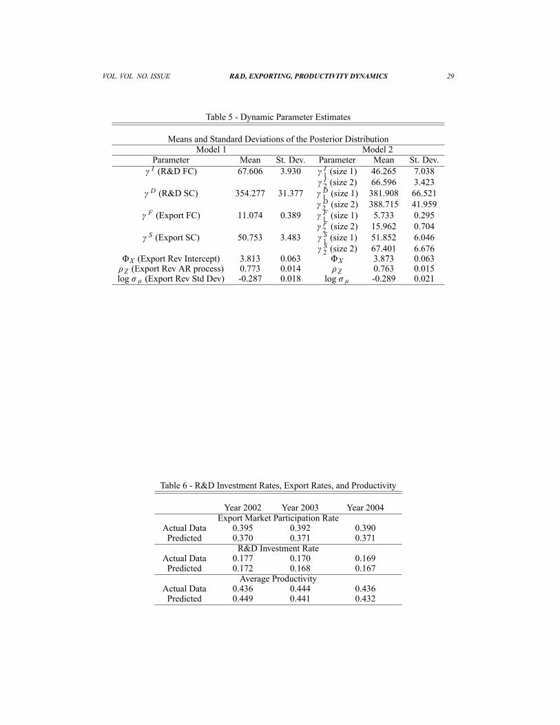
VOL. VOL NO. ISSUE R&D, EXPORTING, PRODUCTIVITY DYNAMICS 29
Table 5 - Dynamic Parameter Estimates
Means and Standard Deviations of the Posterior DistributionModel 1 Model 2
Parameter Mean St. Dev. Parameter Mean St. Dev. I (R&D FC) 67.606 3.930 I1 (size 1) 46.265 7.038
I2 (size 2) 66.596 3.423 D (R&D SC) 354.277 31.377 D1 (size 1) 381.908 66.521
D2 (size 2) 388.715 41.959 F (Export FC) 11.074 0.389 F1 (size 1) 5.733 0.295
F2 (size 2) 15.962 0.704 S (Export SC) 50.753 3.483 S1 (size 1) 51.852 6.046
S2 (size 2) 67.401 6.6768X (Export Rev Intercept) 3.813 0.063 8X 3.873 0.063�Z (Export Rev AR process) 0.773 0.014 �Z 0.763 0.015log �� (Export Rev Std Dev) -0.287 0.018 log �� -0.289 0.021
Table 6 - R&D Investment Rates, Export Rates, and Productivity
Year 2002 Year 2003 Year 2004Export Market Participation Rate
Actual Data 0.395 0.392 0.390Predicted 0.370 0.371 0.371
R&D Investment RateActual Data 0.177 0.170 0.169Predicted 0.172 0.168 0.167
Average ProductivityActual Data 0.436 0.444 0.436Predicted 0.449 0.441 0.432
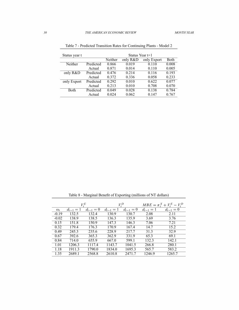
30 THE AMERICAN ECONOMIC REVIEW MONTH YEAR
Table 7 - Predicted Transition Rates for Continuing Plants - Model 2
Status year t Status Year t+1Neither only R&D only Export Both
Neither Predicted 0.866 0.019 0.110 0.008Actual 0.871 0.014 0.110 0.005
only R&D Predicted 0.476 0.214 0.116 0.193Actual 0.372 0.336 0.058 0.233
only Export Predicted 0.292 0.010 0.622 0.077Actual 0.213 0.010 0.708 0.070
Both Predicted 0.049 0.028 0.138 0.784Actual 0.024 0.062 0.147 0.767
Table 8 - Marginal Bene�t of Exporting (millions of NT dollars)
V Et V Dt MBE D � Xt C V Et � V Dt!t dt�1 D 1 dt�1 D 0 dt�1 D 1 dt�1 D 0 dt�1 D 1 dt�1 D 0-0.19 132.5 132.4 130.9 130.7 2.08 2.11-0.02 138.9 138.5 136.3 135.9 3.69 3.760.15 151.8 150.9 147.3 146.3 7.06 7.210.32 179.4 176.3 170.9 167.4 14.7 15.20.49 245.3 235.6 228.9 217.7 31.3 32.90.67 392.6 365.3 362.9 331.9 65.3 69.10.84 714.0 655.9 667.0 599.1 132.3 142.11.01 1206.3 1117.4 1143.7 1041.5 266.8 280.11.18 1911.3 1790.0 1834.0 1695.3 565.7 583.21.35 2689.1 2568.8 2610.8 2471.7 1246.9 1265.7

VOL. VOL NO. ISSUE R&D, EXPORTING, PRODUCTIVITY DYNAMICS 31
Table 9 - Export Policy Functions: Pr.et D 1jet�1; dt�1/
!t et�1 D 1 et�1 D 0 et�1 D 1 et�1 D 0dt�1 D 1 dt�1 D 1 dt�1 D 0 dt�1 D 0
-0.19 0.156 0.032 0.157 0.032-0.02 0.246 0.055 0.248 0.0560.15 0.365 0.098 0.369 0.0990.32 0.518 0.178 0.523 0.1810.49 0.710 0.309 0.718 0.3170.67 0.895 0.485 0.907 0.5030.84 0.969 0.653 0.980 0.6931.01 0.988 0.749 0.994 0.7851.18 0.997 0.835 0.999 0.8731.35 0.997 0.874 0.999 0.901
Table 10 - Costs of Exporting and R&D (millions of NT dollars)
Mean Export Costs among Exportersa Mean R&D Costs among Investorsb!t Fixed Cost Sunk Cost Fixed Cost Sunk Cost-0.19 0.97 1.036 1.32 1.34-0.02 1.61 1.80 2.06 2.120.15 2.64 3.33 3.41 3.590.32 4.18 6.50 6.55 7.280.49 6.21 12.32 12.83 15.640.67 8.50 21.06 24.01 33.740.84 9.86 30.72 36.28 60.781.01 10.35 37.17 43.49 86.611.18 10.67 43.54 49.35 113.931.35 10.70 47.02 48.26 114.87a. For plants with dt�1 D 1b. For plants with et D 1

32 THE AMERICAN ECONOMIC REVIEW MONTH YEAR
Table 11 - Marginal Bene�t of R&D Investment (millions of NT dollars)
EVtC1.dt D 1; et / EVtC1.dt D 0; et / MBR!t et D 1 et D 0 et D 1 et D 0 et D 1 et D 0-0.19 142.2 140.7 139.3 137.6 2.8 3.2-0.02 150.2 147.9 145.8 142.9 4.5 5.00.15 166.2 162.1 158.6 153.7 7.6 8.40.32 200.3 192.1 184.6 175.1 15.7 17.00.49 278.6 262.5 244.3 224.6 34.3 37.90.67 447.3 417.5 371.2 333.0 76.1 84.50.84 797.2 749.5 654.2 583.3 143.0 166.31.01 1320.2 1255.6 1105.7 1004.1 214.5 251.51.18 2065.7 1985.2 1773.5 1637.5 292.2 347.71.35 2883.8 2802.5 2575.2 2425.5 308.6 377.0
Table 12 - R&D Policy Functions: Pr.dt D 1jet ; dt�1/
!t et D 1 et D 1 et D 0 et D 0dt�1 D 1 dt�1 D 0 dt�1 D 1 dt�1 D 0
-0.19 0.041 0.007 0.046 0.008-0.02 0.063 0.011 0.070 0.0120.15 0.101 0.018 0.109 0.0200.32 0.182 0.036 0.192 0.0390.49 0.329 0.075 0.347 0.0820.67 0.566 0.155 0.590 0.1690.84 0.777 0.265 0.812 0.2961.01 0.872 0.360 0.899 0.3991.18 0.940 0.455 0.959 0.5041.35 0.928 0.451 0.951 0.505

VOL. VOL NO. ISSUE R&D, EXPORTING, PRODUCTIVITY DYNAMICS 33
Table 13 - Plant Response to Exogenous Increase in Export Market Size
Year 2 5 10 15Endogenous productivity: !i t D g.!i t�1; di t�1; ei t�1/C � i t
Change in Proportion of Exporters 5.2 9.0 10.0 10.2Change in Proportion of R&D Performers 2.5 3.5 4.1 4.7Percentage Change in Mean Productivity 0.5 1.5 3.7 5.3
Endogenous productivity: !i t D g.!i t�1; di t�1/C � i t
Change in Proportion of Exporters 2.0 3.9 4.0 4.4Change in Proportion of R&D Performers 1.8 2.6 3.5 4.0Percentage Change in Mean Productivity 0.0 0.8 1.9 2.9
Endogenous productivity: !i t D g.!i t�1; ei t�1/C � i t
Change in Proportion of Exporters 3.4 5.9 7.2 7.6Percentage Change in Mean Productivity 0.0 0.0 1.2 1.8
Exogenous productivity !i t D g.!i t�1/C � i t
Change in Proportion of Exporters 4.6 5.7 5.8 5.5