R&D and the Incentives from Merger and …faculty.tuck.dartmouth.edu/.../gordon-phillips/rd_acquisitions.pdfR&D and the Incentives from Merger and AcquisitionActivity ... R&D and the

[17:53 25/10/2012 OEP-hhs109.tex] Page: 1 1–45

R&D and the Incentives from Merger andAcquisition Activity

Gordon M. PhillipsUniversity of Southern California and NBER

Alexei ZhdanovUniversity of Lausanne and Swiss Finance Institute

We provide a model and empirical tests showing how an active acquisition market affectsfirm incentives to innovate and conduct R&D. Our model shows that small firms optimallymay decide to innovate more when they can sell out to larger firms. Large firms mayfind it disadvantageous to engage in an “R&D race” with small firms, as they can obtainaccess to innovation through acquisition. Our model and evidence also show that theR&D responsiveness of firms increases with demand, competition, and industry mergerand acquisition activity. All of these effects are stronger for smaller firms than for largerfirms. (JEL G34, L11, L22, L25, O31, O34)

We examine how the market for mergers and acquisitions affects the decisionto conduct research and development (R&D) and innovate. We argue thatan active acquisition market encourages innovation, particularly by smallfirms in an industry. Instead of conducting R&D in-house, large firms canoptimally outsource R&D investment to small firms and then acquire those thatsuccessfully innovate. Successful innovation makes firms attractive acquisitiontargets, and exit through strategic sales becomes an important motivation tocontinue to spend on R&D.

Recent articles describe how acquisitions are often attempts by large firms togrow by buying innovation (Forbes 2008; Bloomberg 2008).1 This acquisitionpotential provides stronger incentives for small firms to engage in R&D. Arecent prominent example is Google. Google made 48 acquisitions of smallerfirms in 2010, six years after it went public, and 60 acquisitions in the previous

Phillips was supported by the National Science Foundation [grants #0823319 and #0965328]. We would like tothank the editor, Andrew Karolyi, and two anonymous referees for their especially helpful comments, and UlfAxelson, Denis Gromb, Naveen Khanna, Erwan Morellec, Urs Peyer, Adriano Rampini, Matthew Rhodes-Kropf,Merih Sevilir, Rajdeep Singh, Toni Whited, and seminar participants at Boston University, HKUST, Insead, theUniversity of Lausanne, the University of New South Wales, Tsinghua University, the 2011 Duke/UNC corporatefinance conference, the 2011 Paris Corporate Finance conference, the 2011 Western Finance Association, and the2011 UBC summer conference for helpful comments and discussion. Send correspondence to Gordon M. Phillips,511 Hoffman Hall, Marshall School of Business, University of Southern California, CA 90089; telephone: (213)740-0598. E-mail: [email protected]. Zhdanov can be reached at [email protected].

1 Companies “cited” as buying others for their innovation include Cisco, General Electric, and Microsoft.

© The Author 2012. Published by Oxford University Press on behalf of The Society for Financial Studies.All rights reserved. For Permissions, please e-mail: [email protected]:10.1093/rfs/hhs109

RFS Advance Access published October 27, 2012 by guest on O

ctober 29, 2012http://rfs.oxfordjournals.org/

Dow

nloaded from

http://rfs.oxfordjournals.org/

[17:53 25/10/2012 OEP-hhs109.tex] Page: 2 1–45

The Review of Financial Studies / v 0 n 0 2012

five years, for a combined total of 108 acquisitions in the six years post–initial public offering (IPO).2 Early in its life, Google bought three smallersearch engines for their technology assets and patents. Each of these companiesoperated search engines with additional features that Google incorporatedinto its online search capabilities.3 Another example is Cisco. To extend itsnetworking offerings, Cisco has purchased 16 computer networking companiesand five computer security companies since 1999.

We present a model and empirical tests showing how an active acquisitionmarket positively affects both small and large firms’ incentives to innovate andconduct R&D. We also show that mergers can be a way to acquire innovationas a substitute strategy for conducting R&D. This motive is distinct from othermotives for acquisitions that include neoclassical theories or agency theoriesof mergers4 and is closest to recent theories and evidence by Rhodes-Kropfand Robinson (2008) and Hoberg and Phillips (2010b) that emphasize assetcomplementarities and product market synergies.

Our model shows why large firms optimally may decide to let small firmsconduct R&D and then subsequently acquire the companies that have successfulinnovated. We show that firms’ incentives to conduct R&D increase withthe probability that they are taken over and how this effect decreases withsize. This result is consistent with evidence that post-acquisition larger firmsinnovate less and with evidence that larger firms conduct less R&D per unitof firm size. Seru (forthcoming) recently finds that patenting goes down post-acquisition and concludes that large conglomerate firms “stifle” innovation,while noting that they are more likely to sign alliances and joint ventures—afact consistent with the outsourcing of R&D. Our interpretation of the decreasein innovative activity is different. Our model and evidence show that R&Dmay optimally decline for large firms but increase for small firms with mergeractivity. Large firms may find it optimal to buy other firms to gain access tosuccessful innovations instead of investing in R&D themselves, while smallfirms face increased incentives to invest in R&D with an active takeover market.An additional benefit of acquisition results from the ability of the merged entityto apply innovation to both the bidder’s and the target’s product ranges.

Specifically, the model provides the following predictions. First, thepossibility of an acquisition induces attempts to innovate by both small and largefirms, but this effect decreases with size as large firms may find it optimal to buysmaller firms that successfully innovate and cannot prevent small firms fromattempting to innovate. The possibility of an acquisition amplifies the potential

2 See “Google Cranks Up M&A Machine,” Wall Street Journal, March 5, 2011.

3 These purchases include Outride (see http://www.google.com/press/pressrel/outride.html), Kaltix (seehttp://en.wikipedia.org/wiki/Kaltix), and Orion (see http://searchengineland.com/google-implements-orion-technology-improving-search-refinements-adds-longer-snippets-17038).

4 See Maksimovic and Phillips (2001) and Jovanovic and Rousseau (2002) for neoclassical and q theories andMorck, Shleifer, and Vishny (1990) for an agency motivation for mergers. See Maksimovic and Phillips (2008)for how conglomerate firms may relax financial constraints in order to acquire other firms.

2

by guest on October 29, 2012

http://rfs.oxfordjournals.org/D

ownloaded from

http://www.google.com/press/pressrel/outride.html

http://en.wikipedia.org/wiki/Kaltix

http://searchengineland.com/google-implements-orion-technology-improving-search-refinements-adds-longer-snippets-17038


[17:53 25/10/2012 OEP-hhs109.tex] Page: 3 1–45

R&D and the Incentives from Merger and Acquisition Activity

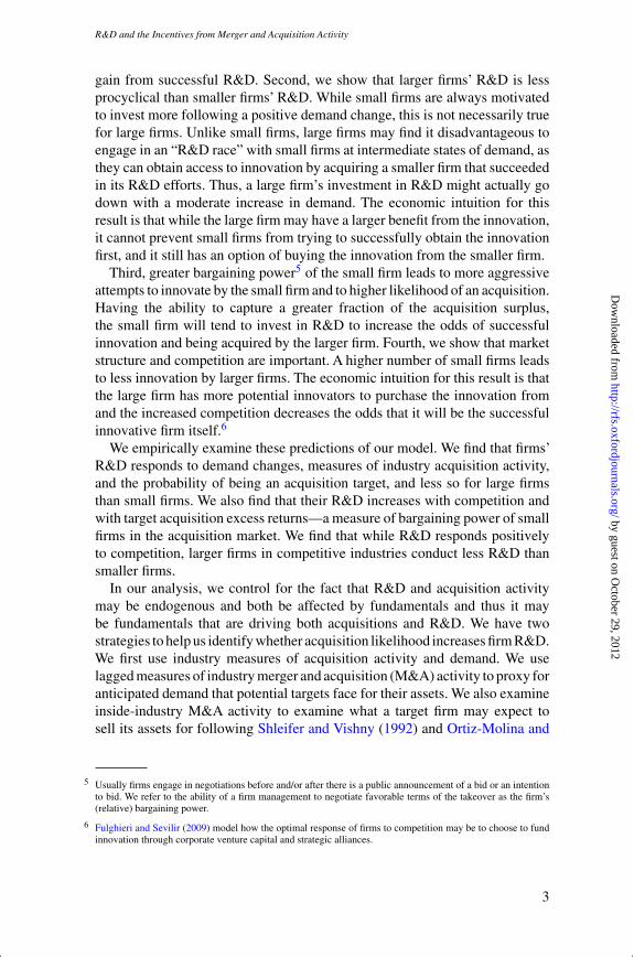
gain from successful R&D. Second, we show that larger firms’ R&D is lessprocyclical than smaller firms’ R&D. While small firms are always motivatedto invest more following a positive demand change, this is not necessarily truefor large firms. Unlike small firms, large firms may find it disadvantageous toengage in an “R&D race” with small firms at intermediate states of demand, asthey can obtain access to innovation by acquiring a smaller firm that succeededin its R&D efforts. Thus, a large firm’s investment in R&D might actually godown with a moderate increase in demand. The economic intuition for thisresult is that while the large firm may have a larger benefit from the innovation,it cannot prevent small firms from trying to successfully obtain the innovationfirst, and it still has an option of buying the innovation from the smaller firm.

Third, greater bargaining power5 of the small firm leads to more aggressiveattempts to innovate by the small firm and to higher likelihood of an acquisition.Having the ability to capture a greater fraction of the acquisition surplus,the small firm will tend to invest in R&D to increase the odds of successfulinnovation and being acquired by the larger firm. Fourth, we show that marketstructure and competition are important. A higher number of small firms leadsto less innovation by larger firms. The economic intuition for this result is thatthe large firm has more potential innovators to purchase the innovation fromand the increased competition decreases the odds that it will be the successfulinnovative firm itself.6

We empirically examine these predictions of our model. We find that firms’R&D responds to demand changes, measures of industry acquisition activity,and the probability of being an acquisition target, and less so for large firmsthan small firms. We also find that their R&D increases with competition andwith target acquisition excess returns—a measure of bargaining power of smallfirms in the acquisition market. We find that while R&D responds positivelyto competition, larger firms in competitive industries conduct less R&D thansmaller firms.

In our analysis, we control for the fact that R&D and acquisition activitymay be endogenous and both be affected by fundamentals and thus it maybe fundamentals that are driving both acquisitions and R&D. We have twostrategies to help us identify whether acquisition likelihood increases firm R&D.We first use industry measures of acquisition activity and demand. We uselagged measures of industry merger and acquisition (M&A) activity to proxy foranticipated demand that potential targets face for their assets. We also examineinside-industry M&A activity to examine what a target firm may expect tosell its assets for following Shleifer and Vishny (1992) and Ortiz-Molina and

5 Usually firms engage in negotiations before and/or after there is a public announcement of a bid or an intentionto bid. We refer to the ability of a firm management to negotiate favorable terms of the takeover as the firm’s(relative) bargaining power.

6 Fulghieri and Sevilir (2009) model how the optimal response of firms to competition may be to choose to fundinnovation through corporate venture capital and strategic alliances.

3



ownloaded from


[17:53 25/10/2012 OEP-hhs109.tex] Page: 4 1–45


Phillips (forthcoming). Second, we also control for endogenous acquisitionprobability by estimating the probability of being an acquisition target usingan plausibly exogenous instrument, unexpected mutual fund flow into and outof stocks, that can affect persistent firm valuation and thus acquisition activitybut not affect firm fundamentals.7

Our research adds to the current academic literature in several areas. First,we provide a new theory for the incentive effects of M&A that has not beenexplored in the literature. The existing literature has emphasized neoclassicalmodels or q-based theories where highly productive firms buy less productivefirms and has also emphasized managerial agency theories of mergers. It alsoadds to the theories that emphasize asset complementarity or product marketsynergies, by emphasizing that new innovations produced through R&D can beused by existing firms with complementary assets. Our paper directly examinesthe effect of acquisition probabilities, market structure, and firm size on R&D.

Second, our model and evidence is consistent with large firms optimallyreducing innovation, letting small firms innovate, and acquiring them later.We focus on the selection effect and how this potential effect may impact pre-acquisition R&D. Other papers focus on treatment effects and examine R&D orpatents post-acquisition. Our evidence is consistent (although the interpretationis different) with other recent papers that examine R&D and patents post-acquisition. Seru (forthcoming) finds conglomerate firms reduce innovationpost-acquisition. Hall (1999) finds no effect on R&D expenditures from mergersof public firms, while a reduction in R&D following going-public transactions.8

A direct implication of our paper is that instead of interpreting low R&D asa sign of managerial inefficiency or myopia, low R&D can be optimal sincethe firm can instead be intending to acquire innovation. Our paper is consistentwith the recent working paper by Bena and Li (2012), who show that largecompanies with large patent portfolios and low R&D expenses are more likelyto be acquirers.

Related literature looks at the relation between competition in productmarkets and innovation, without paying attention to acquisitions. Vives(2008) provides a detailed overview of theoretical and empirical work.Recently, Fulghieri and Sevilir (2011) theoretically model the ex ante effectsof mergers and competition on innovation. They model how a reductionin competition through mergers reduces employee incentives to innovate.The empirical evidence is favorable to the positive effect of competition

7 See Edmans, Goldstein, and Jiang (2012) for the description of and successful use of this instrument. We thankthem for sharing this mutual fund flow instrument with us.

8 Note that our model and evidence are about small firms optimally deciding to sell out. We do not model agencyconflicts nor anti-takeover amendments that are common for larger firms that may be subject to conflicts betweenmanagers and shareholders. See Atanassov (2009) and Chemmanur and Tian (2010) for articles that deal withanti-takeover devices or laws. The anti-takeover laws passed in the United States apply more to large firmtakeovers in more mature industries as they reduce post-acquisition asset sales and are thus not relevant foracquisitions of smaller innovative firms. Also note that these state-level anti-takeover laws were not passed inCalifornia or Texas, two states with a high technology focus.

4



ownloaded from


[17:53 25/10/2012 OEP-hhs109.tex] Page: 5 1–45


on innovation, including Baily and Gersbach (1995), Nickell (1996), andBlundell, Griffin, and Van Reenen (1999). However, most of these papers lookat productivity rather than R&D. Theoretical work seems to support a negativerelation between innovation and competitive pressure. Standard industrialorganization theory predicts that innovation should decline with competition, asmore competition reduces the monopoly rents that reward successful innovators(Dasgupta and Stiglitz 1980). Other theoretical papers suggest a positive(Aghion et al. 2001) or U-shaped relation (Aghion et al. 2002) betweeninnovation and product market competition. We complement and extend thisliterature by focusing on the effect of a potential acquisition on firm innovationincentives.9

Overall our contribution is to focus on the trade-off for large firmsbetween innovating themselves or acquiring small firms that have successfullyinnovated. Acquiring firms that have successfully innovated can be a more-efficient path to obtaining innovation than innovating directly oneself. Weillustrate this effect in a theoretical model and provide rigorous empiricaltests. Second, we generate new empirical predictions regarding procyclicalityof R&D investments and their relation to firm size, the effect of potentialacquisitions on R&D, the link of R&D to industry structure, and the effectof bargaining power and asset liquidity on small firms’ R&D decisions.

1. The Model

We present a model that allows us to draw empirical predictions about therelation between R&D, acquisitions, and firm size. We begin the model witha simple utility function for consumers who value product variety but arewilling to substitute between products. In the base version of the model,we assume heterogeneous products and price (Bertrand) competition.10 Webelieve this type of competition fits the case of many industries such ascomputer networking, cell phones, and consumer products, among others,where companies compete based on product differentiation. We define theproduct space broadly, with specific features that can be patented that represent“local products,” which may affect the demand for existing products. Our ideais that multiple firms can try for a particular product characteristic ex ante yetonly one will obtain the particular product characteristic with a patent. Ex post,one firm innovating does not preclude product differentiation across existing or

9 Our paper is also related to the literature that studies the procyclicality of R&D (e.g., Barlevy 2007 and Aghionet al. 2008).

10 In the online appendix we also examine an alternative competition mechanism, Cournot competition, wherebyfirms produce homogeneous products and innovation results in cost savings, and find similar results. UnderCournot competition with similar competitors, mergers will not take place as rival firms expand output after themerger. This result is a well-known Cournot-merger paradox (Salant, Switzer, and Reynolds 1983). However,the literature (Gaudet and Salant 1992 and Zhou 2008, among others) has shown that under Cournot competitionwith cost savings mergers will take place. In our setting, if the innovation produces large cost savings, mergerswill take place with positive demand shocks.

5



ownloaded from


[17:53 25/10/2012 OEP-hhs109.tex] Page: 6 1–45


new products as the patented product/characteristic, when obtained, may affectthe demand for other firms’ existing products. The rationale is that areas of theproduct space are large enough to contain subareas with differentiated products,each with their own particular differentiation. Thus ex post competition ischaracterized by product differentiation. What is required is that the cross-partial price elasticity of demand is not zero and not infinity. Thus, changesin one product’s price or characteristic affect the other product’s demand butthere is not perfect competition.

The previously cited examples of Google purchasing smaller search enginesfor the different ways they conduct searches and the different features theyoffer in their search engines fits the assumption of differentiated products. Toextend its networking offerings, Cisco has purchased 16 computer networkingcompanies and five computer security companies since 1999. Since 2004,Google has bought many advertising firms (Admeld, Admob) and even theAndroid software firm, which allows it to develop and extend its advertisingbusiness. Note that Admeld and Admob were close competitors of Googleand not just supply-chain related. Google had moved into the business sellingadvertising through display ads, not directly connected to searches, as displayads appear after you visit a firm’s Web site. Admeld and Admob were alsoselling advertising through display ads. From an advertiser’s perspective, adsoffered through search or display ads on the Internet are differentiated productsthat they purchase. The pricing for one product affects the demand for theother, but they serve the same function of getting the advertiser’s messageout to consumers. Admeld and Admob had a different technology for sellingdisplay ads and as such had product extensions that were useful to Google andwere viewed by many industry participants as competitors with differentiatedproducts.11

Our model captures both heterogeneous products and the intensity of productmarket competition in a simple setting. We believe that this setting provides arealistic background for the issues of interest, as a positive effect of innovationby a small firm is likely to result in a shift in consumers’demands. However, ouranalysis is robust to the scenario in which innovation results in cost savings andfirms compete in quantities (see the online appendix for results). We study onelarge firm and up to two small firms, but the model can potentially be extendedto allow additional firms. We allow each firm to innovate and introduce a new

11 Admeld’s Web site (http://www.admeld.com/about/overview/) highlights the technology and methods thatthey use to display advertising on Web sites. As their Web site states, “Admeld was first to introduce theprivate exchange (November 2010), first to optimize mobile (January 2010), and the first to launch anad monitoring browser plugin (March 2009). Quite simply, our engineers are building things better andfaster to keep our clients on the cutting edge.” Many articles have discussed the potential for decreasedcompetition post-deal, including one stating, “So what is the Admeld deal really about for Google? Thecompany is seeking to expand its monopoly power in search advertising to other aspects of online advertising,where Google is already the 800 lb. gorilla between its acquisition of DoubleClick in 2008, and Google’smulti-billion-dollar annual AdSense business” (http://www.fairsearch.org/acquisitions/approval-for-admeld-deal-could-make-google-another-category-killer/).

6



ownloaded from

http://www.admeld.com/about/overview/

http://www.fairsearch.org/acquisitions/approval-for-admeld-deal-could-make-google-another-category-killer/


[17:53 25/10/2012 OEP-hhs109.tex] Page: 7 1–45


product, but they can also choose to purchase other firms instead of innovatingthemselves.

1.1 General setup1.1.1 Consumers. We follow Vives (2000, 2008) and Bernile, Lyandres, andZhdanov (2012) and consider an industry with n (n∈{2,3}) firms. Initially, eachproduct is produced by a single firm. There is a representative consumer, with ageneral quadratic utility function that allows for concavity in consumer utilityas she consumes more of any given product and also allows for differentiatedproducts captured by the parameter γ, the degree of substitutability among theproducts:

U (−→q )=√

x

m∑i=1

αiqi − 1

2

⎡⎣ m∑

i=1

βq2i +2

∑j �=i

γ qiqj

⎤⎦, (1)

where αi >0 represents consumer preferences for product i, β measures theconcavity of the utility function, γ represents the degree of substitutabilitybetween products i and j, and m is the number of different products in themarket. We assume that β >γ >0,12 αi >αj implies that the consumer prefersproduct i to product j, but still consumes both products as long as they areimperfect substitutes (γ <β). In (1),qi is consumption of good i,n is the numberof active firms in the industry, and, thus, the number of available products, andx is the stochastic shock to the representative consumer’s utility. γ >0 ensuresthat the products are (imperfect) substitutes. The higher the γ, the more alike arethe products and the more intense is competition in the industry. Furthermore,we follow Vives (2008) and assume that, in addition to the products above, thereis a numeraire good (or money), which represents the rest of the economy, andincome is large enough that the income and wealth constraints never bind andall income effects are captured by consumption of the numeraire good. In whatfollows, we normalize β to 1. (The results are insensitive to this normalization.)In this setting, as γ approaches 1, the consumer becomes indifferent betweenthe products and is better off having a high quantity of the product with thelower price and none of the others.

1.1.2 Production technology. There are n (n∈{2,3}) firms in the industry.Firms have a similar production technology, but we allow heterogeneity inthe size of firms, with each firm initially endowed with capital Ki . The firms’production functions are of the Cobb-Douglas specification with two factors:

qi =√

KiLi, (2)

where qi is the quantity produced by firm i, and Li is the amount of the secondfactor (e.g., labor) employed by firm i.

12 This assumption ensures that the utility function is concave. For high values of γ, the consumer is better offhaving a high quantity of one product and none of the other products rather than moderate amounts of all products.

7



ownloaded from


[17:53 25/10/2012 OEP-hhs109.tex] Page: 8 1–45


The cost of one unit of labor is denoted pl . The amount of capital is fixed,hence labor is the only variable input. Given this specification, firm i’s cost ofproducing qi units is

Ci(qi)=q2

i

Ki

pl. (3)

This specification results in profit functions of the following form:

πi =qipi −Ci(qi). (4)

Firms are heterogeneous in the amount of capital. There is one big dominatingfirm with capital K1 and one or two small firms with capital K2,(3) <K1 each.In what follows, we assume that pl =1 (the results are insensitive to thisassumption).

1.1.3 R&D and innovation. Each firm in the industry has an option to investin R&D to potentially obtain and develop an innovative technology at a cost ofRDi. If one firm invests in R&D, then it develops the innovation with 100%certainty. If multiple firms invest in R&D, the probability that any individualfirm develops the innovation decreases to 1/n.13 The innovative technology,once developed, can be brought to the market through commercialization. Forthe sake of simplicity, we assume that commercialization is costless, but weobtain similar results under the assumption that commercialization requiresa certain cost of Ii to be incurred by firm i. Bringing to market the productbased on this innovation results in an enhanced product that results in increasedconsumer utility for the product, as reflected in an increase of the parameterαi from αi1 to αi2, where αi1 <αi2. For simplicity, we assume that αi1 =α andαi2 =α′, i ∈{1,2,3}.

1.1.4 The acquisition market. The big firm, whether or not it has acquiredthe innovative technology, has an option to take over one small firm. Weassume (for simplicity to focus on innovation) that there are no economiesof scale and that the merged firms utilize all the pre-merged firms’ capitaland do not reallocate capital between their production facilities (or that it isprohibitively costly to do so). Nevertheless, there are two consequences ofan acquisition on the profit of the merged entity (and its competitors, if any).First, the two firms are now able to coordinate their pricing strategies, whichleads to greater market power and increases equilibrium prices and profits.Second, the merged entity can apply innovation to its entire product line,resulting in an increase of the consumer preference parameter from α to α′ for

13 In section 2 of the online appendix, we also analyze the case in which the probability of innovating successfullydoes not depend on the number of firms that attempt to innovate and multiple firms can develop the innovation.Our results are robust to this case.

8



ownloaded from


[17:53 25/10/2012 OEP-hhs109.tex] Page: 9 1–45


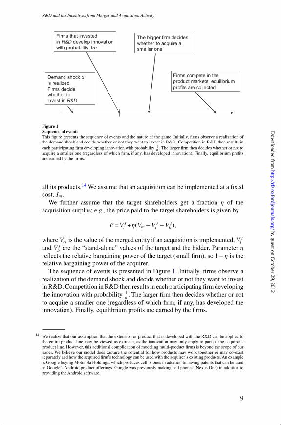
Figure 1Sequence of eventsThis figure presents the sequence of events and the nature of the game. Initially, firms observe a realization ofthe demand shock and decide whether or not they want to invest in R&D. Competition in R&D then results ineach participating firm developing innovation with probability 1

n . The larger firm then decides whether or not toacquire a smaller one (regardless of which firm, if any, has developed innovation). Finally, equilibrium profitsare earned by the firms.

all its products.14 We assume that an acquisition can be implemented at a fixedcost, Im.

We further assume that the target shareholders get a fraction η of theacquisition surplus; e.g., the price paid to the target shareholders is given by

P =V st +η(Vm−V s

t −V sb ),

where Vm is the value of the merged entity if an acquisition is implemented, V st

and V sb are the “stand-alone” values of the target and the bidder. Parameter η

reflects the relative bargaining power of the target (small firm), so 1−η is therelative bargaining power of the acquirer.

The sequence of events is presented in Figure 1. Initially, firms observe arealization of the demand shock and decide whether or not they want to investin R&D. Competition in R&D then results in each participating firm developingthe innovation with probability 1

n. The larger firm then decides whether or not

to acquire a smaller one (regardless of which firm, if any, has developed theinnovation). Finally, equilibrium profits are earned by the firms.

14 We realize that our assumption that the extension or product that is developed with the R&D can be applied tothe entire product line may be viewed as extreme, as the innovation may only apply to part of the acquirer’sproduct line. However, this additional complication of modeling multi-product firms is beyond the scope of ourpaper. We believe our model does capture the potential for how products may work together or may co-existseparately and how the acquired firm’s technology can be used with the acquirer’s existing products. An exampleis Google buying Motorola Holdings, which produces cell phones in addition to having patents that can be usedin Google’s Android product offerings. Google was previously making cell phones (Nexus One) in addition toproviding the Android software.

9



ownloaded from


[17:53 25/10/2012 OEP-hhs109.tex] Page: 10 1–45


1.2 Solution

The equilibrium prices and profits of firms in the industry depend on whichfirm has successfully innovated (if any) and on whether an acquisition occurs.In the following subsections, we allow for a large firm and a small firm withvarying degrees of bargaining power. We start with a case when a merger isprecluded and then proceed by incorporating a possibility of an acquisition. Wealso analyze an industry with two small firms and one big firm to illustrate theeffect of increasing competition.

Case 1: One small firm and one large firm: No acquisition is possible

To find the equilibrium profits, we first differentiate the utility function withrespect to quantities and set the derivatives equal to prices. Solving the resultingsystem of equations for quantities gives the demand functions

q1 =

√x (α1 −α2γ )−p1 +p2γ

1−γ 2, (5)

q2 =

√x (α2 −α1γ )−p2 +p1γ

1−γ 2. (6)

The inverse demand functions are linear in prices. We then substitute thesefunctions into profit functions (4), differentiate with respect to prices (firmsmaximize their profits by setting prices competitively), set the derivatives equalto zero, and solve the resulting system of equations. This produces equilibriumprices, provided in the appendix. We then substitute equilibrium prices backinto the inverse demand functions to get equilibrium quantities, then into profitfunctions (4) to obtain equilibrium profits.

Figure 2 plots the equilibrium profit of a firm as a function of “consumerpreferences”; equivalently, this can be thought of as a firm’s “product innovationparameter,” αi, for its product, that of its competitor, αj , the relative size of thetwo firms, K1/K2, and the degree of product differentiation, γ.The comparativestatics are based on the following parameter values: K1 =10, K2 =1, γ =0.5,

α1 =10, α2 =10. For each graph, we compute the profits with these valuesbut vary one of them as indicated on the x-axis. Consistent with intuition,equilibrium profit of one firm increases in its own product innovation parameterαi, and decreases with its product substitutability γ, its rival’s capitalizationKj, and its rival’s product innovation parameter, αj .

Let us denote the equilibrium profit of firm i by πi(Ai,Aj ), where Ai =NI if firm i decides not to invest in R&D and Ai =I if it invests. Lemma 1establishes certain relations between equilibrium profits in different scenarios.These relations prove useful in the subsequent analysis of the optimal R&Dand acquisition policies.

10



ownloaded from


[17:53 25/10/2012 OEP-hhs109.tex] Page: 11 1–45


Figure 2Equilibrium profits: two firms, no acquisition possibleThis figure presents the equilibrium profit of a firm as a function of its “innovation parameter,” α, the capitalratio of the firms K1/K2, and the degree of product differentiation, γ, for the following set of input parameters:K1 =10, K2 =1, γ =0.5, α1 =10,α2 =10. For each graph, we compute the profits with these values but vary oneof them as indicated on the x-axis. Consistent with intuition, equilibrium profit of one firm increases in its owninnovation parameter αi , and decreases with its product substitutability γ , its rival’s capitalization Kj , and itsinnovation parameter αj .

Lemma 1. Let K1 >K2 and Im =0.15 Then, the following inequalities hold:

a) π1(I,NI )>π1(NI,NI )>π1(NI,I ).

b) π2(NI,I )>π2(NI,NI )>π2(I,NI ).

c) Let γ =0.5. Then π1(I,NI )−π1(NI,NI )>π2(NI,I )−π2(NI,NI ).

d) π1(I,NI )−π1(NI,I )> π2(NI,I )−π2(I,NI ).

e) Let γ =0.5 and K2 =1. Then, there exists μ>1 and αh >>α such thatfor K1/K2 >μ and α<αi <αh, the following inequality holds:

π1(I,NI )−π1(NI,I )

2>π2(NI,I )−π2(NI,NI ).

15 Our results hold for positive merger cost Im >0. Assuming a positive merger cost is only useful to illustrate theprocyclicality of takeovers.

11



ownloaded from


[17:53 25/10/2012 OEP-hhs109.tex] Page: 12 1–45


f) Let γ =0.5 and K2 =1. Then, there exists μ1 >1 such that for K1/K2 >

μ1 the following inequality holds:

2(π1(I,NI )−π1(NI,NI ))>π2(NI,I )−π2(I,NI ).

g) The following relation holds: π2(NI,I )−2π2(NI,NI )+π2(I,NI )>0.

Proof. See Appendix. �Parts a and b of Lemma 1 simply state that the profit of a firm increases if

it innovates and decreases if a competitor implements innovation, as shownin Figure 1. Parts c and d state that a successfully implemented innovationhas a greater effect on the profit of the larger, more capital-intensive firm.While we impose some parameter restrictions in parts c, e, and f, we alsoperform numerical simulations to investigate the robustness of our results andfind that in general the statements of Lemma 1 hold for a large set of reasonableparameter values, and even when some of these statements are violated, ourmajor predictions still go through. See the online appendix for details.16

Let us now introduce the following threshold boundary parameters. Theseboundary parameters are useful as they define important thresholds that shapefirms’ equilibrium R&D policies:

x1 =RD

π1(I,NI )−π1(NI,NI ); x2 =

RD

π2(NI,I )−π2(NI,NI );

x3 =2RD

π2(NI,I )−π2(I,NI ); x4 =

2RD

π1(I,NI )−π1(NI,I ).

Note that Lemma 1 a) and b) ensure that all these values are positive, whileLemma 1 e) ensures that x4 <x2. Lemma 1 c) ensures that x1 <x2. Lemma 1d) ensures that x4 <x3. Lemma 1 f) ensures that x1 <x3. Lemma 1 g) ensuresthat x2 <x3.

The optimal R&D policy of each firm depends on the current state of demandx and on the actions of its opponent. Each firm first decides whether it wants toinvest in R&D. If neither firm invests, then neither develops the innovation andthe profits of the two firms are given by π1(NI,NI ) and π2(NI,NI ). If onlyone firm invests in R&D, then it acquires the new technology with certainty.If both firms invest in R&D, then each of them has a 50% chance of obtainingthe patent. The successful firm then commercializes the innovation.

Proposition 2 defines the equilibrium R&D strategies of the two firms in theabsence of takeovers.

16 Lemma 1 part c and Lemma 1 part f hold for a large set of parameter values. For example, both these conditionshold if K1 =10;a =10; 0.1�γ �0.9; 1�K2 �9; 11�α′ �30. Lemma 1 part e is, however, more restrictive. Itholds well when the ratio of the capital stocks of the two firms K1/K2 is relatively high. For example, it holds forthe following parameter combinations: K1 =10;a =10; 0.25�γ �0.75; K2 �1; 11�α′ �18, or K1 =10;a =10;0.05�γ �0.95; K2 �0.5; 11�α′ �30. We believe that our story is more relevant for large firms acquiringmuch smaller ones, and less for a merger of similar firms. However, numerical analysis suggests that even whenlemma 1 part e is violated, our major predictions still obtain.

12



ownloaded from


[17:53 25/10/2012 OEP-hhs109.tex] Page: 13 1–45


Proposition 2. Assume that conditions a–f of Lemma 1 hold. Then, thereare three Nash equilibria in pure strategies, depending on the value of x. Inparticular, for x <x1, the only Nash equilibrium is (NI,NI ) (no firm invests).For x1 <x <x3, the only Nash equilibrium is (I,NI ) (the big firm invests andthe small firm does not). For x >x3, the only equilibrium is (I,I ) (both firmsinvest).

Proof. See Appendix. �Figure 3 presents the equilibrium strategies of the two firms in the space

(α′,x). The results in Figure 3 are based on the following set of parametervalues: K1 =10, K2 =1, γ =0.5, α =10, α′ =15,RD1 =RD2 =15. There arethree regions in Figure 3. For very low states of x, the NPV of investing in R&Dfor the big firm, NPV1, is negative, and so is the NPV of investing in R&Dfor the small firm, NPV2, so both firms optimally choose not to invest (regionI). For sufficiently high values of x, NPV1 becomes positive and the big firminvests; while NPV2 is still negative, the benefit of applying innovation to thecapital stock of the small firm is less valuable than that of the big firm with moreabundant capital (region II). Finally, for even higher states of x, the small firmchooses to join the R&D race with the big firm, as the value of the option tojoin becomes positive (region III). Regions I and II are separated by thresholdx1, while regions II and III are separated by threshold x3. As shown in Figure 3,the incentive to invest in innovation for both firms is greater when the benefitof innovation α′ is high.

Figure 3Equilibrium strategies: two firms, no acquisition possibleThis figure presents the equilibrium investment thresholds of the two firms in the case when an acquisition isprecluded, as functions of the innovation parameter α′. The set of input parameters is as follows: K1 =10, K2 =1,

γ =0.5, α1 =α2 =10,α′ =15,RD1 =RD2 =15. No firm invests in Region I, only the big firm invests in Region II,and both firms invest in Region III. Regions I and II are separated by x1; Regions II and III are separated by x3.

13



ownloaded from


[17:53 25/10/2012 OEP-hhs109.tex] Page: 14 1–45


Case 2: One small firm and one large firm: Acquisitions are possible

We now assume that the big firm has an option to acquire the small one. Asuccessful acquisition results in a single firm in the industry, which sets pricesto maximize its total (monopoly) profits. If either the small or the big firm hasdeveloped the innovation, then the merged firm will commercialize it. Note thatthe merged entity still produces two separate products, and demand for eachproduct will be characterized by the parameter α =α′. The profit of the mergedentity is given in the appendix. We denote by πm(I ) the profit of the mergedentity if it implements the innovation and by πm(NI ) its profit if it does notimplement the innovation.

The equilibrium investment choices of firms are found similarly to theprevious case by comparing expected firm values in different scenarios. Whendeciding whether or not to invest in R&D, the big firm now takes into accountthe possibility of acquiring the small firm if the latter develops the innovation.Likewise, the small firm incorporates the possibility of being acquired by thebig firm in its optimization problem.

Proposition 3 establishes the equilibrium R&D strategies of the two firms ifan acquisition is possible.

Proposition 3. Assume η=0 (the big firm captures 100% of thetakeover surplus). Also assume that the following conditions hold:πm(I )−πm(NI )>π1(I,NI )−π1(NI,NI )17 and π2(NI,I )−π2(NI,NI )>π2(NI,NI )−π2(I,NI ).18 If takeovers are possible, then the following arethe Nash equilibria in pure strategies. If x <x1m, where

x1m =RD

πm(I )−πm(NI )+π2(NI,NI )−π2(I,NI ),

then the only Nash equilibrium is (NI,NI ) (no firm invests). If x1m <x <x2,

then the only Nash equilibrium is (I,NI ) (big firm invests). If x2 <x <x3, thenthere are two pure-strategy Nash equilibria: (NI,I ) (small firm invests andbig firm does not) and (I,NI ) (big firm invests and small firm does not). Inaddition, there is a mixed-strategy equilibrium in which the big firm invests withprobability p1 and the small firm invests with probability p2 (these probabilitiesare determined in the appendix). If x >x3, then the only equilibrium is (I,I )(both firms invest).

17 This condition stipulates that the acquisition benefit is greater for the merged entity than it is for the big firm (asa stand-alone entity). It is intuitive and holds for a large set of reasonable parameter values.

18 This condition also holds for a large set of reasonable parameter values. It is also intuitive and implies that thepositive effect of its own innovation on the profit of the small firm is greater in absolute value than the negativeeffect due to the large firm innovating. See the online appendix for details.

14



ownloaded from


[17:53 25/10/2012 OEP-hhs109.tex] Page: 15 1–45


Figure 4Equilibrium strategies: two firms, an acquisition is possibleThis figure presents the equilibrium investment thresholds of the two firms in the case when an acquisition ispossible, as functions of the innovation parameter α′. The set of input parameters is as in Figure 3. In addition,the relative bargaining power of target is assumed to be zero (η=0). At low states of the demand shock x, bothfirms prefer not to invest in R&D (Region I). In Region II, only the big firm invests. In Region III, there are twopure-strategy Nash equilibria: (small firm invests, big firm does not; big firm invests, small firm does not) and amixed-strategy equilibrium (the small firm invests with probability φ2 and the big firm invests with probabilityφ1; φ2 and φ1 are determined in the appendix). Both firms invest in Region IV.

Proof. See Appendix. �Figure 4 illustrates the equilibrium innovation strategies of the two firms.

There are two important differences between Figures 3 and 4. First, innovationby the big firm starts at a lower state of demand x, because the potential benefitof innovation is greater—the big firm has an option to acquire the small oneand apply the innovation to both its capacity and production and the productioncapacity acquired from the non-innovating small firm so x1m is less x1 (see proofof Proposition 2 in the appendix). Second, there is a region in which there isa pure-strategy equilibrium, in which the small firm innovates while the bigfirm does not, and another mixed-strategy equilibrium, in which the small firminnovates with a certain probability φ2. (For the set of parameter values usedin Figure 4, the state of demand x =1.5, and the innovation parameter α′ =12,

the corresponding probabilities are φ1 =0.58 and φ2 =0.91.)Note that while our modeling framework does not allow us to determine

which firm is going to invest in the intermediate region, any advantage in termsof flexibility or speed of reacting to current market conditions would lead to afirst-mover advantage and would make the more inert firm less likely to invest.Since it cannot outpace the faster firm, it would be forced not to invest. It isreasonable to think of small firms as being more flexible and able to adaptfaster to changes in the market. In this case, by investing first a small firmwould rule out the (I,NI ) equilibrium and the mixed-strategy equilibrium.

15



ownloaded from


[17:53 25/10/2012 OEP-hhs109.tex] Page: 16 1–45


Furthermore, numerical results show that in the mixed-strategy equilibrium,the probability of the small firm investing is typically higher than that of thelarge firm. On the other hand, for larger, capital-intensive R&D projects, thelarge firm can potentially commit more capital than the small one and that cangive it a competitive edge and result in the (I,NI ) outcome.

Overall, by comparing Figures 3 and 4, we conclude that the possibility oftakeover intensifies the small firm’s R&D investment. Indeed, in region III inFigure 4 there is no equilibrium in which the small firms invest if takeoversare not allowed (Figure 3), while there are multiple equilibria in this regionif takeovers are possible (Figure 4). Furthermore, when we analyze below (inextensions of the model) the case where bargaining power of the target mayvary, for some values of the bargaining parameter η, there is a region in which(NI,I) is the only equilibrium.

We proceed to analyze the effect of takeover cost Im on the dynamics oftakeovers. A takeover always results in a reduction in the number of firmsand therefore in greater market power and increased combined profits for thecombined firms, as the firms can now internalize their pricing decisions. Thus,πm(I )>π1(I,I )+π2(I,I ). As shown by Proposition 2, at high values of x bothfirms optimally decide to innovate even if takeovers are precluded, because thebenefit of innovation is proportional to x. Given the bargaining power parameterη, the fraction of the surplus captured by the large firm is η(πm(I )−π1(I,I )−π2(I,I ))x and increasing in x. Clearly, for

x >Im

η(πm(I )−π1(I,I )−π2(I,I )),

the takeover benefit outweighs the cost and the large firm initiates the takeover.On the other hand, for very low x the benefit of the takeover is not enoughto compensate for the cost. Thus, if x < Im

η(πm(NI )−π1(NI,NI )−π2(NI,NI )) , takeoverdoes not occur. This leads to the procyclicality of takeovers. Takeovers alwayshappen at sufficiently high values of x and never happen at low x, as long asthe takeover cost Im is positive. This logic is summarized in Proposition 4 andis illustrated in Figure 5.

Proposition 4. If Im >0, then takeovers are procyclical.This result is consistent with the large theoretical literature on acquisitions

and capital reallocation (e.g., Lambrecht 2004; Morellec and Zhdanov 2005;Eisfeldt and Rampini 2006) and supported by empirical evidence (Mitchelland Mulherin 1996; Maksimovic and Phillips 2001; Harford 2005). Figure 5plots the demand threshold, x, at which the acquisition just becomes profitable,as a function of the acquisition cost Im. We solve the model numerically forpositive values of Im.Acquisition is optimal for the states of demand exceedingx. As Figure 5 shows, acquisitions are procyclical and acquisition thresholdsincrease in the cost of merger Im.Note that in general there are two acquisitionthresholds that divide the space (x,Im) into three different regions. In the bottom

16



ownloaded from


[17:53 25/10/2012 OEP-hhs109.tex] Page: 17 1–45


Figure 5Acquisition thresholdsThis figure presents the equilibrium acquisition strategy as a function of the demand shock x and the takeovercost Im. The set of input parameters is as in Figure 3. Above the higher boundary (Region III), an acquisitionoccurs with certainty. Between the lower and the upper thresholds (Region II), an acquisition is optimal onlyif the small firm obtains the innovation. Below the lower threshold (Region I) acquisition never occurs. Thus,the probability of an acquisition is positively related to the state of the demand shock x and acquisitions areprocyclical.

region (region I), acquisitions never occur. The cost of merger is too high inthat region for an acquisition to be optimal. In the top region (region III),acquisitions occur with probability one. In that region, even if the big firmdevelops the innovation it still wishes to acquire the small one because it canapply the innovation to its capital stock as well. On the other hand, it willalso benefit from reduced industry competition. In the middle region (regionII), an acquisition occurs only if the small firm has successfully developed theinnovation. Because of the relatively large cost of an acquisition, the big firmdoes not find it optimal to acquire the small one if the former has accessedthe innovation through its own R&D program. It can commercialize withoutperforming an acquisition. By contrast, if the small firm obtains the innovativetechnology, the big firm has more incentives to initiate an acquisition, becauseit will also result in gaining access to the innovation. Note that in our modela merger always has a positive effect on the combined profit of the mergedentity even if the innovation is not commercialized. This pure market powereffect arises because competition becomes less intense following the mergerand the equilibrium profits rise. Therefore, even in the absence of innovation,takeovers occur with 100% certainty at very high states of x.

1.3 Extensions of the modelIn this section, we allow for varying bargaining power of the small firm and formultiple small firms and analyze the effect of these features on firm incentives

17



ownloaded from


[17:53 25/10/2012 OEP-hhs109.tex] Page: 18 1–45


to invest in R&D. We start with the analysis of varying bargaining power.For our analysis, it is convenient to introduce the following notations:

x1η =RD

η(π1 (I,NI )−π1 (NI,NI ))+(1−η)(πm (I )−πm (NI )+π2 (NI,NI )−π2 (I,NI ))

x5η =2 RD

(1−η)[π2 (NI,I )−π2 (I,NI )]+η[π1 (I,NI )−π1 (NI,I )]

x2η =RD

(1−η)(π2 (NI,I )−π2 (NI,NI ))+η(πm (I )−πm (NI )+π2 (NI,NI )−π2 (I,NI )).

Proposition 5 establishes the equilibrium R&D strategies of the two firms if anacquisition is possible and the small firm has positive bargaining power.

Proposition 5. Assume 0<η<1 (the small firm captures a fraction of thetakeover surplus). Also assume that the following inequalities hold:19 x2η <

x5η and x1η <x5η. If takeovers are possible, then the following are the Nashequilibria in pure strategies:

a) If x1η <x2η, then if x <x1η, the only Nash equilibrium is (NI,NI )(no firm invests). If x1η <x <x2η, the only Nash equilibrium is (I,NI )(only big firm invests). If x2η <x <x5η, then there are two pure-strategyNash equilibria: (NI,I ) (small firm invests and big firm does not) and(I,NI ) (big firm invests and small firm does not). In addition, there is amixed-strategy equilibrium in which the big firm invests with probabilityp1 and the small firm invests with probability p2. If x >x5η, the onlyequilibrium is (I,I ) (both firms invest).

b) If x2η <x1η, then if x <x2η, the only Nash equilibrium is (NI,NI ) (nofirm invests). If x2η <x <x1η, the only Nash equilibrium is (NI,I ) (onlysmall firm invests). If x1η <x <x5η, then there are two pure-strategyNash equilibria: (NI,I ) (small firm invests and big firm does not) and(I,NI ) (big firm invests and small firm does not). In addition, there is amixed-strategy equilibrium in which the big firm invests with probabilityp1 and the small firm invests with probability p2. If x >x5η, the onlyequilibrium is (I,I ) (both firms invest).

Proof. See Appendix. �

Corollary 6. x5η is decreasing in η; furthermore, if πm(I )−πm(NI )>π1(I,NI )−π1(NI,NI ), then x1η is increasing in η and x2η is decreasing in η.

Proof. The first statement follows from Lemma 1 d). The last two statementsfollow from Lemma 1 a) and b) and the definitions of x1η and x2η. �

19 These inequalities hold for a large set of reasonable parameter values. See the online appendix for a discussion.

18



ownloaded from


[17:53 25/10/2012 OEP-hhs109.tex] Page: 19 1–45


Corollary 6 implies that the small firm invests more aggressively as itsbargaining power, η, increases. When η goes up, x2η declines. Note that x2η

is the border of the region in which there are equilibria with the small firminvesting, so this region expands downward when η increases. Furthermore, asseen in Figure A.1 of the online appendix, for low enough η,x2η falls below x1η

and there appears a region in which the only equilibrium entails the small firminvesting.At higher states of demand, the small firm is again more aggressive asx5η is decreasing in η.The big firm responds to a greater bargaining power of thesmall firm in a different way: on one hand, it invests more aggressively at higherstates of demand (x5η goes down); on the other, it invests less aggressively atlow states of demand (x1η goes up). Because it has to share the takeover surpluswith the small firm, it becomes less motivated to invest when expected profitsare low.

Figure 6Equilibrium strategies: two firms with target bargaining powerFigure 6 presents the equilibrium investment thresholds of the two firms in the case when an acquisition ispossible, as functions of the innovation parameter α′. The set of input parameters is as follows: K1 =10, K2 =1,

γ =0.5, α1 =α2 =10,α′ =15,RD1 =RD2 =15. In addition, the relative bargaining power of target shareholdersη=0.5. In Region II, only the big firm invests. In Region III, there are three Nash equilibria: two pure-strategyones (small firm invests, the big firm does not; big firm invests, small firm does not) and a mixed-strategyequilibrium. Both firms invest in Region IV. It follows from comparing with Figure 4 that greater bargainingpower of the potential target (small firm) increases its innovation incentives.

Figure 6 shows the equilibrium R&D strategies of the firms when the smallfirm has greater bargaining power and captures a fraction of acquisition surplus,η=0.5.

There are two important differences between Figure 4 (η=0) and Figure 6(η=0.5). First, the intermediate region (region III) is much wider. Since thesmall firm gets a share of the acquisition benefit, it is more motivated to engagein R&D, so it could sell out to the big firm at a higher price. Because of a

19



ownloaded from


[17:53 25/10/2012 OEP-hhs109.tex] Page: 20 1–45


high potential payoff in the event of successful innovation and subsequentacquisition, the small firm is motivated to pursue an aggressive R&D strategy.Second, the boundary at which both firms decide to invest in R&D shifts down,consistent with Corollary 6.

In addition, we show in section 2 of the online appendix that furtherincreasing the bargaining power of the small firm gives rise to a new region inwhich the only equilibrium is the one in which only the small firm invests (andthe big firm does not; see Figure A1 in the online appendix).

Finally, we consider the case when there are multiple small firms and onelarge firm. Due to the complexity of this case, we solve it numerically. Weanalyze this case in section 3 of the online appendix. Analysis of this case givesus two new results. First, the aggregate investment in R&D is higher whenthere are two small firms in the industry than when there is only one small firm.Second, and more importantly, a small firm has a stronger motivation to engagein R&D and get a better chance of being acquired by the larger firm. A smallfirm that does not become a takeover target will face intensified competitionwith the bigger entity (formed in result of the acquisition of its rival) that alsocommercializes the new technology. While it faces potential competition in theR&D market with the other small firm, it has a stronger incentive to becomea takeover target and to avoid becoming an outsider. On the other hand, thebig firm is less motivated to invest when there are two small firms, given moreaggressive investment in R&D by the small firms and because it has a lowerprobability of success facing competition with two firms. Therefore, the big firmprefers to let one of them develop an innovative technology and consequentlyacquire the innovation through an acquisition. As a consequence, there exists aregion that is shown graphically in which in the only pure-strategy equilibrium,both small firms invest, while the big firm does not.

1.4 Discussion of modeling assumptions

In this section, we discuss the main modeling assumptions that we have made inthe paper. We also discuss the potential limitations, robustness, and extensionsof these assumptions.

First, we assume in our analysis that the amount of R&D spending is fixedand also that it is the same for the large and the small firm. An interestingextension would be to examine continuous investment whereby each extradollar spent on R&D increases the probability of success. Incorporating thisassumption would, however, make the model much more complex. We believe,however, that our major qualitative results will still obtain in this case. R&Dwill still be procyclical (though the relation between R&D spending and x willbe continuous and not binary as in our model). If acquisitions are allowed,then the same economic mechanism will apply and the big firm will have lessincentives to invest in R&D at intermediate demand states as it will have anoption to obtain access to innovation through acquisition. At high levels of

20



ownloaded from


[17:53 25/10/2012 OEP-hhs109.tex] Page: 21 1–45


demand, big and small firms will invest in R&D given the large gains fromsuccessful innovation.

Second, we assume that the probability of successful innovation equals 1/n,

where n is the number of firms that invest in R&D. As shown in the onlineappendix, our general results hold if the probability of successful innovationby a firm is independent of the number of other firms that invest in R&D. Wethank the referee for suggesting this alternative specification.

Third, we need to impose some restrictions on parameter values to be ableto analytically prove some of our results. However, further analysis shows thatour results are robust to reasonable variations of parameter values. We presentthis additional analysis in the online appendix.

Finally, in generating our predictions, we implicitly assume that a wide rangeof the values of x is feasible so there is a positive probability of finding the firmin various regions in Figures 3, 4, and 6. Thus, substantial variation in demandis required to generate the full spectrum of our predictions.

1.5 Predictions of the model

Below we summarize the empirical predictions we generate with the model.We test these predictions in the empirical section of this paper.

P1. Acquisitions are procyclical.

This result is illustrated in Figure 5 and follows from the fact thatequilibrium profits as well as the benefit of acquisitions are increasingin the demand level x. It is supported by Proposition 4.

P2. Firm R&D is procyclical.

This prediction follows from Propositions 2 and 3 and is illustrated inFigures 3 and 4. Higher values of demand make it more attractive forfirms to invest in R&D either to keep innovation to themselves or tobecome an attractive acquisition target, if an acquisition is possible.

P3. Large firms’ R&D is less procyclical than small firms’ R&D.

Unlike small firms, large firms may find it disadvantageous to engagein an “R&D race” with small firms at intermediate states of demand, asthey can obtain access to innovation by later acquiring a small firm thatsucceeded in its R&D efforts. It follows from Proposition 2 that thereis a non-monotonic relation between the large firm’s investment policyand the state of x. This is also illustrated in Figure 4. It always investsin regions II and IV in Figure 4, never invests in region I, and there areequilibria in region III in which it does not invest either. Furthermore,Propositions 4 and 5 show that there exists an intermediate region inwhich only the big firm invests. A similar situation occurs with twosmall firms, as illustrated in Figure A.2 of the online appendix. Theregions in which the big firm invests alternate with those in which it

21



ownloaded from


[17:53 25/10/2012 OEP-hhs109.tex] Page: 22 1–45


does not, giving rise to a non-monotonic relation between demand andthe large firm’s R&D investment.20

P4. Possibility of being acquired induces innovation efforts by large andsmall firms, but especially by the small firms.

This prediction is illustrated in Figures 3 and 4 and follows from thefact that the possibility of an acquisition amplifies the potential gainfrom successful R&D. It follows from Lemma 1, part g, that x2 <x3,

so there always exists a region (x2,x3) such that there is no equilibriumwith the small firm investing if takeovers are precluded, while there areequilibria in the same region that involve the small firm investing iftakeovers are allowed. Thus, possibility of being acquired leads to moreR&D by small firms.

P5. Greater bargaining power of the small firm leads to more aggressiveinnovation efforts by the small firm.

This prediction follows from the fact that, having the ability to capturea greater fraction of the acquisition surplus, the small firm will tend toinvest in R&D more aggressively to increase the odds of being acquiredby the larger firm. This prediction follows from Proposition 5 andCorollary 6. It is also illustrated in Figure 6 and Figure A.1 in the onlineappendix. The region in which only the big firm invests shrinks withincreased bargaining power of the small firm, as shown in Figure 6, andcompletely disappears with very high bargaining power of the small firm(η=0.9, fig A.1), while the region in which both firms invest expands.

P6. Increased product market competition leads to more R&D but less sofor large firms.

The intuition for this prediction is similar to that of prediction 3. Withmore small firms in the industry, big firms become less motivated toinvest in their own R&D programs (and face intense competition withsmall firms) and are more inclined to let small firms innovate and thenacquire those that innovate successfully. This result is illustrated inFigure A.2 of the online appendix. We show that small firms invest moreaggressively when facing competition with another small firm in bothR&D and acquisition markets. The regions with at least one equilibriumin which a small firm invests expand. In addition, there emerges a regionin which in the only pure-strategy Nash equilibrium, both small firmsinvest, while the big firm does not.

20 To generate this prediction, we implicitly assume that a wide range of the values of x is feasible, including thosein regions I–IV in Figure 4. Thus, a substantial variability of demand conditions is necessary for the mechanismsin our model to work. We thank the referee for pointing this out.

22



ownloaded from


[17:53 25/10/2012 OEP-hhs109.tex] Page: 23 1–45


2. Data and Empirical Methodology

2.1 SampleOur data come from the merged CRSP-Compustat Database, the Securities DataCorporation (SDC), the St. Louis Federal Reserve Economic Database (FRED),and the Census of Manufactures. We start with the merged CRSP-CompustatDatabase and exclude companies in the financial (SIC codes 6000 to 6999)and utilities (SIC codes 4900 to 4999) industries. Our initial sample includes12,941 firms operating in 181 different three-digit SIC industries and 117,151firm-year observations during the period 1984–2006. We merge with thesedata a sample of mergers and acquisitions from Securities Data Corporation(SDC) from the same period of time. We also drop companies for which weare unable to compute acquisition liquidity or our main control variables. Ourfinal sample of firms with matched industry demand data, and with lagged andcontemporaneous non-zero assets, includes 11,288 firms with 84,471 firm-yearobservations.

Table 1 presents the summary statistics for our main variable, annual R&Dexpenditures scaled by sales,21 and also the annual acquisition rate by differentsize groups. PanelAshows that the highest R&D activity as a percentage of salesis concentrated among firms with below-median size. R&D for firms betweenthe 25th and 50th percentiles of market capitalization is 2.4% of sales. Giventhat market capitalization reflects growth options and R&D may capture manygrowth options, the fact that R&D is very low at the lowest size decile is notsurprising.At the highest size decile, R&D is also a low fraction of stock marketcapitalization, consistent with many growth options being already exercised forthese large firms. Panel B shows the acquisition rates of firms based on theirstock market capitalization. Firms in the lowest size groups are more likely tobe acquired.

2.2 Identification strategy: Acquisition activity and industry demandand supply

In our analysis, we wish to examine the effect of expected acquisition activityon firm R&D. We face a fundamental identification problem that R&D andacquisitions may both result from fundamental demand conditions. Firmsconduct R&D not just because they may sell out to another firm but alsobecause of fundamental demand conditions. Acquisitions as well also respondto these fundamental demand conditions. Thus, to separate out the effect ofexpected acquisition activity on R&D, we have to control for industry demandand also find exogenous asset liquidity shift variables or instruments that

21 We note that the distribution of R&D/Sales is skewed to the right, with many firms reporting zero R&D. Weexamined whether this had an effect on our regression results and found that it did not. Our results hold usingquantile regressions at the 50th (median regression) and 75th percentiles, and the results with these quantileregressions are actually slightly stronger than the results we report. We also examine R&D scaled by assets, andour results, including later regression results, are robust to this alternative scaling.

23



ownloaded from


[17:53 25/10/2012 OEP-hhs109.tex] Page: 24 1–45


Table 1R&D and acquisition summary statistics

Panel A: R&D/Sales

Variable Mean Median Std. Dev. N

R&D/Sales, size < 10% 0.266 0.000 1.716 7348R&D/Sales, 10% < size < 25% 0.487 0.016 2.793 11018R&D/Sales, 25% < size < 50% 0.669 0.024 3.125 18381R&D/Sales, 50% < size < 75% 0.450 0.015 2.324 18381R&D/Sales, 75% < size < 90% 0.153 0.001 1.063 11019R&D/Sales, 90% < size < 100% 0.056 0.004 0.271 7348

Panel B: Acquisition rate

Annual acquisition rate, size < 10% 0.162 0.186 0.087 23Annual acquisition rate, 10% < size < 25% 0.099 0.098 0.026 23Annual acquisition rate, 25% < size < 50% 0.095 0.097 0.026 23Annual acquisition rate, 50% < size < 75% 0.086 0.080 0.025 23Annual acquisition rate, 75% < size < 90% 0.070 0.071 0.034 23Annual acquisition rate, 90% < size < 100% 0.055 0.051 0.028 23

Table 1 reports summary statistics for R&D scaled by sales and number of acquisitions by year for different sizegroups. After assigning firms to size groups by year, we average the rates by year and then average over all theyears in our data. Size is defined as the log of the market equity value.

affect acquisition activity but do not affect firm-level corporate R&D. Wethus construct several different measures of industry asset liquidity. We alsoconstruct the direct probability that a firm is a target using an instrumentalvariable approach. Thus, we do not rely solely on exogenous variables or ourinstrumental variable approach. This dual approach provides reassurance thatour results are robust to different methods to control for endogeneity.

To begin, we discuss our controls for fundamental industry demandconditions. We then discuss our measures of acquisition activity and liquidityin the market for acquisitions. Finally, we discuss our instrumental variableregression approach where we endogenize the probability that a firm is anacquisition target and the instruments we use to help with identification.

2.2.1 Industry demand conditions. To capture industry demand, we usemeasures of downstream demand that we obtain from the Federal Reserve onthe value of industrial production seasonally by industry, converted into fourdigit SIC codes. The industrial production data are publicly available seriesavailable from the Federal Reserve based on data from the Census Bureau.22 Weaggregate these measures to the three-digit level and then calculate the annualchange for each year. We then link these data to each industry by “downstream”industries using the input output matrix of the U.S. economy from the Bureauof EconomicAnalysis in the closest lagged census year (this matrix is publishedevery five years) using the Bureau of Economic Analysis “use” tables, where

22 These data are available at http://www.federalreserve.gov/releases/g17/table1_2.htm, starting from the year 1919.

24



ownloaded from

http://www.federalreserve.gov/releases/g17/table1protect LY1extunderscore 2.htm


[17:53 25/10/2012 OEP-hhs109.tex] Page: 25 1–45


a downstream industry is one that uses 1% or more of the industry’s output.23

Given that most industries sell to multiple downstream industries, to constructour final measure of changes in demand we weight the percentage changeof each downstream industry by the percentage sold to that industry at thethree-digit level. For industries that sell directly to consumers, we use thechange in consumer income in real dollars. For industries that sell directly tothe government, we use the change in government military expenditures in realdollars as the downstream demand index, as military expenditures are plausiblyexogenous to each industry’s shipments itself.

We construct two measures of demand changes using these data. First,following Maksimovic and Phillips (2001), Vdshock is the detrended annualpercentage change in the downstream industry using the input-output matrix. Todetrend this variable, we regress it on industry and year fixed effects indicatorvariables and then take the residual from this regression. The detrended variablerepresents the “shock” or unanticipated change to demand. Vexpand is a“discretized” version of Vdshock, which equals one when Vdshock is positiveand zero otherwise. We use both variables in our tests because of potentialnon-linearities in the effect of increases in demand on R&D. In our model, theresponse of R&D intensity to changes in demand is highly non-linear.

2.2.2 Industry acquisition activity. Our first measure of expected assetliquidity in the market for acquisitions is a three-year lagged average measureof industry asset transactions, broken up into inside and outside industrytransactions. It follows Schlingemann, Stulz, and Walkling (SSW) (2002) in thatSSW examine how a firm’s probability of selling is related to overall industryacquisition activity. We differ from SSW as we average the lagged industryM&A activity to capture what a firm might expect will be the potential marketfor its assets, following Ortiz-Molina and Phillips (forthcoming), who examinethe effect of inside liquidity on a firm’s cost of capital. This measure capturesthe historical liquidity of an industry’s assets using the value of past M&Aactivity in the firm’s industry over the last three years (we also examine thelast five years, and our results are robust to this change). Shleifer and Vishny(1992) argue that a high volume of transactions in an industry is evidence ofhigh liquidity because the discounts that sellers must offer to attract buyers aresmaller in more active resale markets.

We thus obtain the value of all M&A activity involving publicly tradedtargets in each three-digit SIC industry and in each year from the Securities DataCorporation (SDC). We include both mergers and acquisitions of assets. For fullfirm purchases, deal value is the purchase price paid to target shareholders. Foracquisition of assets, deal value is the reported purchase price. Acquisitions

23 Input output tables are from the Bureau of Economic Analysis Web site and are publicly available at http://www.bea.gov/industry/#io. The latest input-output table at the time of our analysis is for 2007. We match thesedata into SIC codes using publicly available correspondence tables.

25



ownloaded from

http://www.bea.gov/industry/#io


[17:53 25/10/2012 OEP-hhs109.tex] Page: 26 1–45


of assets are important conceptually and economically to our argument.Conceptually there are many firms who develop R&D in divisions and thensell that division. In our sample, overall acquisitions of assets are particularlyimportant as they comprise approximately 75% of the total deals by number.

If SDC does not report corporate transactions in an industry-year, we setthe value of transactions equal to zero. We then scale the value of transactionsin the industry by the total book value of assets in the industry, and averagethis ratio over the past three years, not including the contemporaneous year.To compute the value of the assets in each industry, we sum the assets inthe industry reported by single-segment firms and the segment-level assetsreported by multiple-segment firms in the Compustat segment data, breakingup the multiple-segment firms into their component industries using the valueof reported assets by their component industries. Averaging over past yearssmooths the temporary ups and downs in M&A activity and allows us to bettercapture the intrinsic saleability of an industry’s assets.24

We decompose our measure of asset liquidity to distinguish between insidebuyers of assets–those who operate in the same three-digit SIC industry as thetarget–and outside buyers–those who do not currently operate in the industry.We use the Compustat Segment tapes to further refine this calculation followingOrtiz-Molina and Phillips (forthcoming). We classify a purchase as an insidepurchase if the buyer has any segments with the same three-digit SIC code asthe assets purchased–checking over each reported SIC code of the target if thetarget reports multiple SIC codes. Inside Industry M&A is the value of M&Aactivity in the industry involving acquirers that operate within the industry,scaled by the book value of the assets in the industry. Outside Industry M&Ais the value of M&A activity in the industry involving acquirers that operateoutside the industry, scaled by the book value of the assets in the industry. Bothof these variables are again averaged over the past five years.

We also calculate the cumulative abnormal announcement return to pasttargets in each industry in the prior year as an additional measure of what atarget firm might expect to receive if they receive a buyout offer. We calculatethe cumulative abnormal return for each past deal in the industry and averageover all deals in each industry at the three-digit SIC code level. Excess returnsare cumulated from 30 days prior to the announcement date of each deal to 10days post-deal. Parameters of the market model (α,β) used to calculate excessreturns are estimated from regressions of each stock return on the S&P marketreturn using trading days -255 to - 31 prior to the announcement date.

2.2.3 The probability of being a target. Our second main measure ofexpected asset liquidity in the market for acquisitions is a firm’s individual

24 Our analysis is unaffected if we use five years of M&A data instead of three years. We have calculated thepersistence of lagged industry M&A and found it to be very persistent. The correlation between 1 and 3-yearslagged inside industry M&A activity is 0.752. The correlation between 1- and 5-year inside M&A activity is0.640. The correlation between 3- and 5-year lagged inside industry M&A activity is .898.

26



ownloaded from


[17:53 25/10/2012 OEP-hhs109.tex] Page: 27 1–45


probability of being an acquisition target. We thus include the target dummyvariable in the R&D regressions and instrument this endogenous variable usingas an instrument a measure of the unexpected mutual fund flow followingEdmans, Goldstein, and Jiang (2012). This method is analogous to a two-stageleast squares method, where the first stage is a linear probability model of theprobability a firm is a target.

We use this second approach as there is the concern that the previous laggedindustry acquisition activity may itself be caused by something fundamentalthat is driving both industry acquisition activity and R&D. For example, ifdemand shocks are persistent, they may affect both the probability of a merger(historically) and may continue to affect the demand for the product. The IVapproach combined with the industry lagged fundamentals provides additionalconfidence in our results and conclusions.

The unexpected mutual flow variable captures the pricing pressure fromchanges in mutual fund holdings that are caused by redemptions that induces themutual fund to sell stocks. This unexpected mutual fund flow has been shownto have persistent valuation effects that Edmans, Goldstein, and Jiang (2012)show extend up to 24 months. It is likely to be exogenous to fundamentals butmay impact acquisition likelihood through a firm’s discount from fundamentalsas it captures deviations from predicted valuation that are caused by investorsredeeming mutual fund shares that subsequently cause the mutual funds to sellstocks. The mutual fund flow instrument has been used successfully recently byEdmans, Goldstein, and Jiang (2012) as an exogenous instrument that affectsfirm’s acquisition probability through the discount or valuation channel. Wetest in the next section whether this variable affects firm R&D only through theprobability of an acquisition and find that this is indeed the case.25

We estimate the regression using an instrumental variable approach (seecommand ivreg2 in Stata). In unreported results, we also used a two-stepgeneralized method of moments (GMM) approach and obtained similar results.Standard errors are estimated that allow for heteroscedasticity and industry-year clustering of the errors. While we use a single-equation instrumentalvariable approach, for general interest and to motivate the other controlvariables for the R&D regression, we also use the results of the first-stagetarget prediction model using a linear probability model. The variables usedin this target prediction model include variables motivated by Ambrose andMegginson (1992), Maksimovic and Phillips (2001), and Harford (2005),as well as the mutual fund flow instrument excluded from the R&Dregressions.

25 Edmans, Goldstein, and Jiang (2012) show that Mfflow only affects takeovers indirectly, through its effect onfirm valuation. It is still a valid instrument for our purpose as long as it is exogenous to fundamentals but affectstakeover probability either directly or indirectly.

27



ownloaded from


[17:53 25/10/2012 OEP-hhs109.tex] Page: 28 1–45


2.2.4 Control variables. The firm-specific control variables included in boththe target prediction regression and the R&D regressions follow the basicspecification of Ambrose and Megginson (1992) and Harford (2005). We lagthese variables one period. These control variables include Log(Cash/Sales),which is the natural log of the ratio of cash to sales, NWCNA, which is networking capital divided by sales, Tangibility, which is the proportion of tangibleassets, and the P-E ratio, which is the price-to-earnings ratio. The institutionalownership variable follows Edmans, Goldstein, and Jiang (2012). Institutionalownership is the percentage of stock owned by institutional investors.

We also include an economy-wide variable to the supply of capital. Weuse the spread between the rate on commercial & industrial (C&I) loans andthe Fed funds rate as a measure for aggregate liquidity following Harford(2005) and also shown by Maksimovic, Phillips, and Yang (forthcoming) toaffect both private and public merger waves. Lown et al. (2000) find thatthis spread is strongly correlated with the tightening of liquidity measuredfrom the Federal Reserve Senior Loan Officer (SLO) survey. We also controlfor industry competition and firm misvaluation or unexplained valuation. Ourmeasure of industry competition is based on the Census Herfindahls as updatedand extended to non-manufacturing industries by Hoberg and Phillips (2010a).The variable “compete” is equal to one minus the Herfindahl index. We alsoexamine if our results are robust to the text-based industry concentrationmeasure developed in Hoberg and Phillips (2011). This later measure is onlyavailable for years 1997 onward, and thus these results are only available for asubset of our sample period.

In addition, several authors have also recently argued that a significantfraction of merger activity of public firms can be explained by misvaluationor unexplained valuation. For example, Rhodes-Kropf, Robinson, andViswanathan (RKRV) (2005) argue that while economic shocks might befundamental determinants of merger activity, misvaluation by public marketsmay determine who buys whom and how mergers are clustered in time. Weadopt a variant of the RKRV measure of firm- and industry-specific unexplainedvaluation and check whether the addition of this variable affects our findings.We label this variable in our tables UV, RKRV to indicate that it is unexplainedvaluation based on the RKRV model. To calculate the measures of unexplainedvaluation, we use model (3) from RKRV, as updated by Hoberg and Phillips(2010a).26 First, we regress log market value of equity on log book valueof equity, net income, an indicator for negative net income, and leverageratio by industry using a historical lagged 10-year rolling window. FollowingHoberg and Phillips, we use only lagged data in the calculation of these

26 As discussed by Rhodes-Kropf, Robinson, and Viswanathan (2005), the key to investigating these effects isobtaining a good measure of misvaluation. Just using reported Tobin’s q cannot distinguish fundamental valuefrom potential misvaluation. Measures of misvaluation are of necessity valuation anomalies relative to a modelof market expectations. While intended to measure misvaluation, they may also pick up the market’s expectationof future performance.

28



ownloaded from


[17:53 25/10/2012 OEP-hhs109.tex] Page: 29 1–45


coefficients to avoid any look-ahead bias. Then, we use the estimated industry-specific regression coefficients to compute the predicted market value of equity,assuming that a firm’s market value at time t is a function of its currentcharacteristics and the industry-specific value of characteristics estimated frompast years. The unexplained valuation measure is then the difference betweenthe actual valuation and the predicted valuation both at time t. For robustnesswe also calculate a second unexplained valuation measure using the valuationmodel from the Pastor and Veronesi (2003) (PV), model 1, as described inHoberg and Phillips (2010a). In our tables, this variable is reported as UV, PV.Firm-level UV, PV is the firm-level unexplained valuation computed based onthe PV model. Firm-level UV, RKRV is the firm-level unexplained valuationcomputed based on the RKRV model. Industry-level UV, RKRV and Industry-level UV, PV are the industry-level unexplained valuation variables based onRKRV and PV, respectively.27

2.3 Summary statisticsTable 2 presents summary statistics for our sample of Compustat Firms.

Our demand variables are presented in the first group. We present thedetrended annual percentage change (Vdshock) in the downstream industryand also its discretized version (Vexpand). We study the effect of both demandshock variables in our regressions.

The second group of variables in Table 2 represents measures of theliquidity in the market for mergers. Industry M&A Activity is the asset liquiditymeasure capturing the value of M&A activity in the industry, while. InsideIndustry M&A is the value of M&A activity involving acquirers from thesame industry. Outside Industry M&A is the value of M&A activity involvingacquirers operating outside the industry. Cum. Abn. announcement return is theindustry-level mean abnormal announcement returns to acquisition targets inthe previous year.

The third group of variables in Table 2 is our unexplained valuation variableswhich may capture either unexplained future growth prospects or misvaluation.The last group of variables is our ownership and the instruments for the targetinstrumental variable regression, unexpected mutual fund flow, from Edmans,Goldstein, and Jiang (2012).

3. Firm R&D Multivariate Results

3.1 R&D and industry M&A activityWe now turn to our main results where we examine firm-level R&D. Weexamine R&D scaled by sales. We examine whether industry merger activityaffects firm R&D. We include variables capturing size, demand changes, and

27 In our sample, the correlation between the PV and RKRV measures is 0.93.

29



ownloaded from


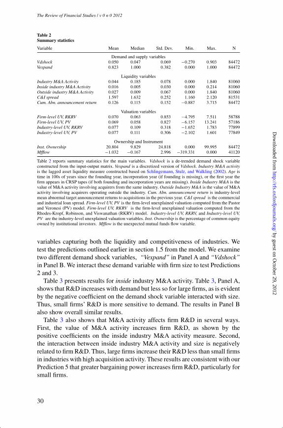
[17:53 25/10/2012 OEP-hhs109.tex] Page: 30 1–45


Table 2Summary statistics

Variable Mean Median Std. Dev. Min. Max. N

Demand and supply variablesVdshock 0.050 0.047 0.069 −0.270 0.903 84472Vexpand 0.823 1.000 0.382 0.000 1.000 84472

Liquidity variablesIndustry M&A Activity 0.044 0.185 0.078 0.000 1.840 81060Inside industry M&A Activity 0.016 0.005 0.030 0.000 0.214 81060Outside industry M&A Activity 0.027 0.009 0.067 0.000 1.840 81060C&I spread 1.597 1.632 0.252 1.160 2.120 81531Cum. Abn. announcement return 0.126 0.115 0.152 −0.887 3.715 84472

Valuation variablesFirm-level UV, RKRV 0.070 0.063 0.853 −4.795 7.511 58788Firm-level UV, PV 0.069 0.058 0.827 −6.157 13.241 57186Industry-level UV, RKRV 0.077 0.109 0.318 −1.652 1.783 77899Industry-level UV, PV 0.077 0.111 0.306 −2.102 1.601 77849

Ownership and InstrumentInst. Ownership 20.804 9.829 24.818 0.000 99.995 84472Mfflow −1.032 −0.167 2.996 −319.331 0.000 41120

Table 2 reports summary statistics for the main variables. Vdshock is a de-trended demand shock variableconstructed from the input-output matrix. Vexpand is a discretized version of Vdshock. Industry M&A activityis the lagged asset liquidity measure constructed based on Schlingemann, Stulz, and Walkling (2002). Age istime in 100s of years since the founding year, incorporation year (if founding is missing), or the first year thefirm appears in CRSP tapes (if both founding and incorporation years are missing). Inside Industry M&A is thevalue of M&A activity involving acquirers from the same industry. Outside Industry M&A is the value of M&Aactivity involving acquirers operating outside the industry. Cum. Abn. announcement return is industry-levelmean abnormal target announcement returns to acquisitions in the previous year. C&I spread is the commercialand industrial loan spread. Firm-level UV, PV is the firm-level unexplained valuation computed from the Pastorand Veronesi (PV) model. Firm-level UV, RKRV is the firm-level unexplained valuation computed from theRhodes-Kropf, Robinson, and Viswanathan (RKRV) model. Industry-level UV, RKRV, and Industry-level UV,PV are the industry-level unexplained valuation variables. Inst. Ownership is the percentage of common equityowned by institutional investors. Mfflow is the unexpected mutual funds flow variable.

variables capturing both the liquidity and competitiveness of industries. Wetest the predictions outlined earlier in section 1.5 from the model. We examinetwo different demand shock variables, “Vexpand” in Panel A and “Vdshock”in Panel B. We interact these demand variable with firm size to test Predictions2 and 3.

Table 3 presents results for inside industry M&A activity. Table 3, Panel A,shows that R&D increases with demand but less so for large firms, as is evidentby the negative coefficient on the demand shock variable interacted with size.Thus, small firms’ R&D is more sensitive to demand. The results in Panel Balso show overall similar results.

Table 3 also shows that M&A activity affects firm R&D in several ways.First, the value of M&A activity increases firm R&D, as shown by thepositive coefficients on the inside industry M&A activity measure. Second,the interaction between inside industry M&A activity and size is negativelyrelated to firm R&D. Thus, large firms increase their R&D less than small firmsin industries with high acquisition activity. These results are consistent with ourPrediction 5 that greater bargaining power increases firm R&D, particularly forsmall firms.

30



ownloaded from


[17:53 25/10/2012 OEP-hhs109.tex] Page: 31 1–45


Table 3R&D regressions with inside industry M&A activity

Panel A: Regressions with Vexpand

Independent Dependent variable :variable R&D expenditures scaled by sales

Vexpand 0.350∗∗∗ 0.327∗∗∗ 0.656∗∗∗ 0.537∗∗∗ 0.508∗∗∗ 0.497∗∗∗ 0.454∗∗∗(0.100) (0.096) (0.135) (0.123) (0.128) (0.131) (0.126)

Log(net assets) −0.117∗∗∗ −0.056∗∗∗ −0.038∗∗∗ −0.029∗∗∗ −0.043∗∗∗ −0.124∗∗∗(0.017) (0.011) (0.009) (0.009) (0.011) (0.025)

Age −0.249∗∗∗ −0.249∗∗∗ −0.220∗∗∗ −0.218∗∗∗ −0.159∗∗∗ −0.194∗∗∗(0.042) (0.042) (0.036) (0.036) (0.033) (0.036)

Vexpand*Log(net assets) −0.075∗∗∗ −0.063∗∗∗ −0.055∗∗∗ −0.055∗∗∗ −0.052∗∗∗(0.019) (0.018) (0.016) (0.017) (0.015)

Inside industry 6.825∗∗ 6.305∗∗ 6.229∗∗ 5.065∗M&A Activity (2.941) (2.928) (2.828) (2.920)

Ins M&A * Log(net assets) −0.665∗∗ −0.621∗∗ −0.620∗∗ −0.514∗∗(0.279) (0.285) (0.261) (0.252)

Compete 0.017∗∗ 0.113∗∗∗(0.007) (0.027)

Compete*Log(net assets) −0.016∗∗∗(0.004)

Firm-level UV, PV 0.141∗∗∗ 0.141∗∗∗ 0.143∗∗∗(0.016) (0.017) (0.017)

Industry-level UV, PV −0.139 −0.133 −0.130(0.116) (0.109) (0.126)

C&I spread 0.423∗(0.254)

Observations 84,471 84,459 84,459 81,047 56,934 51,001 49,233R-squared 0.017 0.033 0.034 0.037 0.034 0.052 0.047Adj. R-squared 0.0165 0.0326 0.0333 0.0369 0.0340 0.0517 0.0462Control variables No No No No No Yes YesYear dummies Yes Yes Yes Yes Yes Yes No

Panel B: Regressions with Vdshock

Vdshock 0.561 0.247 1.078∗ 1.044∗∗ 0.708 0.705 0.682(0.435) (0.440) (0.594) (0.517) (0.543) (0.568) (0.573)

Log(net assets) −0.118∗∗∗ −0.109∗∗∗ −0.079∗∗∗ −0.066∗∗∗ −0.080∗∗∗ −0.163∗∗∗(0.017) (0.018) (0.013) (0.013) (0.017) (0.033)

Age −0.252∗∗∗ −0.256∗∗∗ −0.227∗∗∗ −0.227∗∗∗ −0.162∗∗∗ −0.197∗∗∗(0.044) (0.044) (0.038) (0.039) (0.032) (0.037)

Vdshock*Log(net assets) −0.195∗∗ −0.222∗∗∗ −0.149∗ −0.146∗ −0.130∗(0.099) (0.083) (0.079) (0.080) (0.075)

Inside industry 7.274∗∗ 6.709∗∗ 6.598∗∗ 5.461∗M&A Activity (2.939) (2.915) (2.830) (2.908)

Ins M&A * Log(net assets) −0.696∗∗ −0.649∗∗ −0.655∗∗ −0.546∗∗(0.272) (0.280) (0.258) (0.253)

Compete 0.020∗∗∗ 0.117∗∗∗(0.007) (0.028)

Compete*Log(net assets) −0.016∗∗∗(0.004)

Firm-level UV, PV 0.141∗∗∗ 0.142∗∗∗ 0.144∗∗∗(0.016) (0.017) (0.017)

Industry-level UV, PV −0.111 −0.104 −0.065(0.115) (0.109) (0.125)

C&I spread 0.423∗(0.256)

Observations 84,471 84,459 84,459 81,047 56,934 51,001 49,233R-squared 0.014 0.031 0.031 0.035 0.032 0.050 0.045Adj. R-squared 0.0142 0.0305 0.0306 0.0345 0.0315 0.0494 0.0442Control variables No No No No No Yes YesYear dummies Yes Yes Yes Yes Yes Yes No

Table 3 reports estimates from R&D regressions. The dependent variable is R&D expense scaled by sales in the previous year.Vdshock is a de-trended demand shock variable constructed from the input-output matrix. Vexpand is a discretized versionof Vdshock. Inside industry M&A Activity is the lagged value of M&A activity involving acquirers from the same industryaveraged over the past three years. Compete is a measure of industry concentration equaling one minus the Herfindahl index.Firm-level UV, PV is the firm-level unexplained computed from the Pastor and Veronesi (PV) model. Industry-level UV,PV is the industry-level unexplained valuation variable. C&I spread is the commercial and industrial loan spread. Controlvariables are tangible assets, cash, and net working capital scaled by sales, price-to-earnings ratio, dividend payment dummy,and institutional ownership. Standard errors are clustered by industry-year. *, **, and *** indicate statistical significance atthe 10%, 5%, and 1% levels, respectively.

31



ownloaded from


[17:53 25/10/2012 OEP-hhs109.tex] Page: 32 1–45


We also examine outside industry M&A purchasing activity. In this case, wesum the value of all M&Aactivity when the acquirer is outside the target’s three-digit SIC code. We find that outside M&A activity does not significantly impactR&D, which is consistent with targets getting lower premiums from outsideindustry purchasers and thus facing lower incentive effects. The coefficientsare significantly lower than those for inside M&A activity. For brevity, we donot present these results for outside industry M&A purchasing activity.

The much stronger, significant results for inside industry M&A activity areconsistent with firms looking to competitor inside-industry firms as potentialacquirers when they evaluate the payoffs of conducting R&D. The overallresults are consistent with Shleifer and Vishny (1992), who predict that insideindustry acquirers are willing to pay more for competitor firms, and withincreased competition from potential buyers leading small firms to invest morein R&D.

Our final test is to examine Prediction 6 that product market competitionincreases firm R&D and more so for small firms. We test this prediction byincluding the variable “Compete” and also interacting it with firm size. Wefind that product market competition increases firm R&D but less so for largefirms. The intuition is that firms have to do more R&D to stay competitivein competitive industries and that small firms incentive to increase R&D isparticular large, either because they can sell out to larger firms or because itenables them to survive in the longer run.

The results in Table 3 are economically significant. For example, a one-standard-deviation decrease in Size (log of net assets) results in an increase inthe R&D-to-Sales ratio by 25.9 percentage points (0.259). Increasing Insideindustry M&A Activity by one standard deviation leads 8.1 percentage pointsmore R&D per dollar of sales. Also, firms spend 24.8 percentage points less(.248) on R&D in times of economic expansions (Vexpand = 1) than in timeswhen industries are contracting (Vexpand = 0).

Table 4 tests Prediction 5 that the bargaining power of target firms increasespotential target firm’s R&D. To test Prediction 5, we examine the averagecumulative abnormal returns to acquisition announcements in the previous yearby other target firms in the same three-digit SIC code industry. The rationaleis that abnormal announcement returns to past industry targets are likely tobe related to the expected return a target will get if they receive a takeoveroffer. The returns are likely to be correlated with the probability that a firmis a target, and we thus do not include other M&A activity variables in thisregression.

The idea is that following periods of high abnormal returns to other firms’acquisition announcements in their industries, target shareholders may naturallyanticipate high returns to their firms and higher bargaining power in the eventof an acquisition. This anticipation may encourage potential target firms tointensify their R&D programs in an effort to create a successful innovation andattract potential bidders.

32



ownloaded from


[17:53 25/10/2012 OEP-hhs109.tex] Page: 33 1–45


Table 4R&D and abnormal announcement returns

Independent Dependent variable:variable R&D expenditures scaled by sales

Vexpand 0.189∗∗∗ 0.112∗(0.065) (0.061)

Log(net assets) −0.010 −0.122∗∗∗ −0.037∗∗∗ −0.144∗∗∗(0.012) (0.019) (0.009) (0.024)

Age −0.177∗∗∗ −0.231∗∗∗ −0.180∗∗∗ −0.234∗∗∗(0.031) (0.039) (0.031) (0.040)

Vexpand*Log(net assets) −0.042∗∗∗ −0.033∗∗∗(0.012) (0.012)

Abn. announcement return 0.593∗∗ 0.520∗∗ 0.579∗∗ 0.511∗∗(0.271) (0.225) (0.267) (0.226)

(Abn. AR)*Log(net assets) −0.086∗∗ −0.077∗∗ −0.085∗∗ −0.076∗∗(0.040) (0.035) (0.039) (0.036)

Compete 0.142∗∗∗ 0.145∗∗∗(0.019) (0.020)

Compete*Log(net assets) −0.016∗∗∗ −0.017∗∗∗(0.003) (0.003)

Vdshock 0.447 0.267(0.508) (0.462)

Vdshock*Log(net assets) −0.152∗∗ −0.129∗∗(0.065) (0.061)

Observations 65,341 58,852 65,341 58,852R-squared 0.140 0.147 0.140 0.147Adj. R-squared 0.138 0.145 0.138 0.145Industry dummies Yes Yes Yes YesControl variables Yes Yes Yes Yes

Table 4 reports estimates from R&D regressions. The dependent variable is R&D expense scaled by sales in theprevious year. Vdshock is a de-trended demand shock variable constructed from the input-output matrix. Vexpandis a discretized version of Vdshock. Log(net assets) is the natural log of the asset value. Age is time in 100s ofyears since the founding year, incorporation year (if founding is missing), or the first year the firm appears inCRSP tapes (if both founding and incorporation years are missing). Abn. AR is industry-level mean cumulativeabnormal announcement returns surrounding acquisition announcements to target firms in the previous year.Compete is a measure of industry competitiveness equaling one minus the Herfindahl index. Standard errors areclustered by industry-year. Control variables are tangible assets, cash, and net working capital scaled by sales,price-to-earnings ratio, dividend payment dummy, and institutional ownership. *, **, and *** indicate statisticalsignificance at the 10%, 5%, and 1% levels, respectively.

Table 4 shows strong support for Prediction 5. The bargaining power oftarget firms strongly increases firm R&D as shown by the significant positivecoefficients on the lagged cumulative abnormal returns ( lagCARsic). The tablealso shows that this effect is larger for smaller firms as the coefficient on theinteraction variable of “lagCARsic” with firm size is negative. Overall thistable supports the conclusion that small firms’ R&D increases strongly whentheir bargaining power in acquisitions increases.

3.2 R&D and the probability of being a targetIn this section, when examining R&D, instead of variables capturing industryM&A activity, we compute a firm-specific measure of the probability a firm isa target. As discussed earlier, there is a potential identification problem given afirm’s predicted probability of being a target and its R&D may respond to thesame demand changes. We thus reexamine our results using as an instrumentunexpected mutual fund redemption flow, Mfflow, for an indicator variable“target” thus capturing the predicted probability of being a target in the R&D

33



ownloaded from


[17:53 25/10/2012 OEP-hhs109.tex] Page: 34 1–45


regression. The assumption is that the instrument, the unexpected mutual flowvariable, only affects R&D by affecting a firm’s probability of being a target.

We first report the results of the first-stage regression where we predict theprobability of being a target. For all specifications, the dependent variableequals one if the firm was a target in an acquisition attempt in a given year andzero otherwise. In Table 5, we estimate a linear probability model to predictthe probability of being a target given that we include interaction variables. Wealso use both fundamental demand and supply variables and other lagged firm-specific variables, Log(Cash/Sales), NWC, which is net working capital dividedby sales, Tangibility, P-E ratio, following the basic specification of Ambroseand Megginson (1992) and Harford (2005). In the last two specifications, weinclude the unexpected mutual fund flow, Mfflow.28

Table 5 shows that coefficients of most variables have the expected signs.The coefficient for Vdshock is positive and marginally significant in regressionswith no year dummies. Vdshock is an annual measure, so inclusion of yeardummies makes it insignificant. Size is positively related to the probability ofbeing taken over; however, size interacted with demand shock is negative—small firms have a relatively higher probability of acquisition at high industrydemand states.

Columns 1 and 2 in Table 5 use the unexpected valuation from RKRV, andcolumns 3 through 6 use the unexpected valuation measures based on model 1 inPastor and Veronesi’s (2003) paper, as adapted by Hoberg and Phillips (2010a).Industry-level unexplained valuation is positive throughout, perhaps reflectingindustries that are viewed as having positive future cash flows or that industriesthat are more positively “misvalued” may have higher acquisition intensity.However, within industries, firm-level unexplained valuation is negative, asacquirers target relatively undervalued firms. These facts are consistent withRKRV and also Maksimovic and Phillips (2001). Finally, the coefficient on C&Ispread is negative as expected, as low spreads make debt capital very accessible.

With respect to our controls, the coefficient on institutional ownership forall specifications is positive, consistent with institutional owners facilitatingacquisitions, and the evidence in Ferreira, Massa, and Matos (2010). In columns5 and 6 in Table 6, we report the results that include our instrument, unexpectedmutual fund redemption flow. Unexpected mutual fund redemption flow,Mfflow, is positive and significantly related to the probability of an acquisition.

We now present the regression for firm R&D with the merger target dummyvariable that is instrumented with Mfflow and its squared value. We alsoinclude all control variables. We estimate the model using a single-equationinstrumental variable estimator allowing for the target indicator variable to be

28 We also estimate the IV model using a probit model as the first stage. These results are presented as Tables 3and 4 of the online appendix. Angrist and Krueger (2001, p. 80) note serious potential concerns with the probittwo-stage model, and as such we rely on the linear probability model. The misspecification worry is that theerrors are not normal.

34



ownloaded from


[17:53 25/10/2012 OEP-hhs109.tex] Page: 35 1–45


Table 5Target prediction regressions

Independent Dependent variable:variable Target dummy

Vdshock 0.018 0.080 0.023 0.087 0.157(0.071) (0.070) (0.071) (0.070) (0.136)

Log(equity value) −0.002 −0.003 −0.005∗ −0.005 −0.013∗∗(0.003) (0.003) (0.003) (0.003) (0.005)

Age 0.087∗∗∗ 0.086∗∗∗ 0.087∗∗∗ 0.086∗∗∗ 0.073∗∗∗(0.010) (0.011) (0.010) (0.011) (0.012)

Vdshock*Log(equity value) −0.010 −0.015 −0.011 −0.015 −0.022(0.015) (0.016) (0.015) (0.016) (0.025)

Firm-level UV, RKRV −0.013∗∗∗ −0.012∗∗∗(0.004) (0.004)

Industry-level UV, RKRV 0.026∗∗∗ 0.018∗∗(0.009) (0.009)

C&I spread −0.048∗∗∗ −0.049∗∗∗ −0.089∗∗∗(0.010) (0.010) (0.013)

Compete 0.033∗∗∗ 0.034∗∗∗ 0.035∗∗∗ 0.036∗∗∗ 0.055∗∗∗∗(0.003) (0.003) (0.003) (0.003) (0.005)

Compete*Log(net assets) −0.006∗∗∗ −0.006∗∗∗ −0.006∗∗∗ −0.006∗∗∗ −0.009∗∗∗(0.001) (0.001) (0.000) (0.001) (0.001)

Cash/Sales −0.002 −0.001 −0.001 −0.001 −0.009∗(0.004) (0.004) (0.004) (0.004) (0.005)

Leverage 0.055∗∗∗ 0.054∗∗∗ 0.055∗∗∗ 0.054∗∗∗ 0.075∗∗∗(0.008) (0.009) (0.008) (0.009) (0.014)

Net WC/Sales 0.014 0.019 0.016 0.021 −0.111∗∗(0.019) (0.018) (0.019) (0.018) (0.043)

Tangibility −0.201∗∗∗ −0.184∗∗ −0.196∗∗ −0.180∗∗ −1.959∗∗∗(0.076) (0.074) (0.077) (0.075) (0.411)

P/E −0.084∗∗ −0.069∗ −0.083∗∗ −0.068∗ −0.092∗∗(0.035) (0.036) (0.035) (0.036) (0.047)

Divd dummy 0.001 0.001 0.001 0.001 −0.002(0.005) (0.005) (0.005) (0.005) (0.007)

InstOwn 0.001∗∗∗ 0.001∗∗∗ 0.001∗∗∗ 0.001∗∗∗ 0.001∗∗∗(0.000) (0.000) (0.000) (0.000) (0.000)

Firm-level UV, PV −0.008∗∗ −0.008∗∗ −0.014∗∗∗(0.003) (0.003) (0.005)

Industry-level UV, PV 0.021∗∗ 0.013 0.016(0.009) (0.009) (0.012)

Mfflow 0.365∗∗∗(0.129)

Observations 49,946 47,433 49,840 47,329 28,575R-squared 0.086 0.078 0.086 0.078 0.075Year dummies Yes No Yes No No

Table 5 presents results from our target prediction regression estimated with a linear probability model. Thedependent variable is the target dummy, equaling one if the firm was a target in an acquisition attempt in agiven year, and zero otherwise. Vdshock is a de-trended version of demand shock variable constructed from theinput-output matrix. Log(market value) is the natural log of the market value of equity. Cash/Sales is the ratio ofcash to sales. Net WC/ Sales is the ratio of net working capital to sales. Tangibility is the ratio of tangible assets.P-E ratio is the price-to-earnings ratio. Divd dummy is a dummy variable equaling one for dividend-paying firmsand zero otherwise. Inst. Ownership is the percentage of common equity owned by institutional investors. C&Ispread is the commercial and industrial loan spread. Firm-level UV, PV is the firm-level unexplained valuationcomputed from the Pastor and Veronesi (PV) model. Firm-level UV, RKRV is the firm-level unexplained valuationcomputed from the Rhodes-Kropf, Robinson, and Viswanathan (RKRV) model. Industry-level UV, RKRV andIndustry-level UV, PV are the industry-level unexplained valuation variables. Standard errors are clustered byindustry-year. *, **, and *** indicate statistical significance at the 10%, 5%, and 1% levels, respectively.

35



ownloaded from


[17:53 25/10/2012 OEP-hhs109.tex] Page: 36 1–45


Table 6R&D with instrumented target from mutual fund flows

Dependent variable:R&D expenditures scaled by sales

Target dummy 3.528∗∗ 3.896∗∗∗ 3.764∗∗∗(1.451) (1.462) (1.394)

Vexpand 0.767∗∗∗ 0.647∗∗∗ 0.666∗∗∗(0.241) (0.206) (0.209)

Log(net assets) −0.316∗∗∗ −0.305∗∗∗ −0.291∗∗∗(0.078) (0.080) (0.075)

Age −0.345∗∗∗ −0.371∗∗∗ −0.364∗∗∗(0.129) (0.128) (0.124)

Vexpand*Log(net assets) −0.108∗∗∗ −0.093∗∗∗ −0.095∗∗∗(0.035) (0.031) (0.031)

Compete 0.083∗∗ 0.041 0.044(0.039) (0.039) (0.038)

Compete*Log(net assets) −0.010∗ −0.004 −0.004(0.005) (0.005) (0.005)

Firm-level UV, RKRV 0.208∗∗∗(0.045)

Industry-level UV, RKRV −0.188∗(0.105)

Firm-level UV, PV 0.181∗∗∗(0.039)

Industry-level UV, PV −0.212∗∗(0.100)

C&I spread 0.908∗∗ 0.904∗∗∗ 0.872∗∗∗(0.360) (0.341) (0.332)

Observations 46,470 44,510 44,410Control variables Yes Yes Yes

Table 6 reports estimates from R&D regressions using instrumental variable approach and Mfflow as an instrumentfor the target indicator variable and all the control variables from the target prediction regression. The dependentvariable is R&D expense scaled by sales in the previous year. Log(net assets) is the log of the asset value. Ageis time in 100s of years since the founding year, incorporation year (if founding is missing), or the first year thefirm appears in CRSP tapes (if both founding and incorporation years are missing). Compete is a measure ofindustry competitiveness equaling one minus the Herfindahl index. C&I spread is the commercial and industrialloan spread. Firm level UV, RKRV is the firm-level unexplained valuation computed from the Rhodes-Kropf,Robinson, and Viswanathan (RKRV) model. Industry-level UV, RKRV is the industry-level unexplained valuationvariable. C&I spread is the commercial and industrial loan spread. Control variables include tangible assets,cash, and net working capital scaled by sales, price-to-earnings ratio, dividend payment dummy, and institutionalownership. Standard errors are clustered by industry-year. *, **, and *** indicate statistical significance at the10%, 5%, and 1% levels, respectively.

endogenous. All models are estimated allowing for robust standard errors withindustry-year clustering.

Table 6 presents the results using the excluded mutual fund flow instrument,Mfflow. The regressions include all control variables that we use in the previouslinear probability target model in Table 5. The results for all specifications showthat firms invest more in R&D when the predicted probability of being acquiredis higher. Results in Table 6 show that takeover probability has an economicallysignificant effect on firms’ R&D. Thus, a 10-percentage-point increase in theprobability of being taken over results in 35.3 to 38.9 percentage points (0.353in column 1, to 0.389 in column 2) more R&D expenditures per dollar of sales.

Firms also invest more in R&D when there are positive demand realizations,particularly for small firms. Firms also invest more in R&D in more competitiveindustries but less for large firms. The variables interacted with firm size show

36



ownloaded from


[17:53 25/10/2012 OEP-hhs109.tex] Page: 37 1–45


Table 7R&D with instrumented target from mutual fund flows and HP concentration measures

Independent Dependent variable:variable R&D expenditures scaled by sales

Target dummy 2.496∗∗ 5.008∗∗ 4.783∗∗ 2.269∗∗ 4.819∗∗ 4.597∗∗(1.110) (2.011) (1.870) (1.064) (1.951) (1.814)

Vexpand 0.897∗∗∗ 0.678∗∗∗ 0.699∗∗∗ 0.868∗∗∗ 0.659∗∗∗ 0.679∗∗∗(0.239) (0.236) (0.235) (0.233) (0.231) (0.230)

Log(net assets) 0.276∗∗∗ 0.104 0.124 0.003 −0.246∗ −0.221∗(0.097) (0.090) (0.086) (0.076) (0.138) (0.126)

Age −0.225∗∗∗ −0.422∗∗∗ −0.413∗∗∗ −0.235∗∗∗ −0.436∗∗∗ −0.427∗∗∗(0.085) (0.158) (0.151) (0.085) (0.160) (0.153)

Vexpand*Log(net assets) −0.116∗∗∗ −0.101∗∗∗ −0.103∗∗∗ −0.112∗∗∗ −0.097∗∗∗ −0.099∗∗∗(0.031) (0.036) (0.036) (0.030) (0.035) (0.035)

HP variable comp. measure 3.885∗∗∗ 3.799∗∗∗ 3.785∗∗∗(1.003) (1.096) (1.078)

HP variable*Log(net assets) −0.534∗∗∗ −0.573∗∗∗ −0.570∗∗∗(0.143) (0.180) (0.175)

HP fixed comp. measure 1.574∗∗∗ 1.102∗∗∗ 1.128∗∗∗(0.331) (0.305) (0.302)

HP fixed*Log(net assets) −0.223∗∗∗ −0.175∗∗∗ −0.179∗∗∗(0.047) (0.051) (0.050)

Firm-level UV, RKRV 0.237∗∗∗ 0.238∗∗∗(0.056) (0.056)

Industry-level UV, RKRV −0.140 −0.143(0.118) (0.119)

Firm-level UV, PV 0.206∗∗∗ 0.207∗∗∗(0.048) (0.048)

Industry-level UV, PV −0.146 −0.150(0.107) (0.108)

C&I spread 0.747∗∗ 0.958∗∗∗ 0.924∗∗∗ 0.693∗∗ 0.914∗∗ 0.880∗∗(0.299) (0.368) (0.356) (0.290) (0.358) (0.347)

Observations 46,401 39,619 39,536 46,420 39,647 39,564Control variables Yes Yes Yes Yes Yes Yes

Table 7 reports estimates from R&D regressions using the instrumental variable approach and Mfflow as aninstrument for the target indicator variable. The dependent variable is R&D expense scaled by sales in theprevious year. Log(net assets) is the log of the asset value. Age is time in 100s of years since the founding year,incorporation year (if founding is missing), or the first year the firm appears in CRSP tapes (if both founding andincorporation years are missing). HP fixed comp. measure is 1-Hoberg-Phillips Herfindahl based on fixed industrydefinitions. HP variable comp. measure is 1-Hoberg-Phillips Herfindahl based on variable industry definitions.C&I spread is the commercial and industrial loan spread. Firm-level UV, RKRV (PV) is the firm-level unexplainedvaluation computed from the Rhodes-Kropf, Robinson, and Viswanathan (RKRV) model. (Pastor and Veronesimodel). Industry-level UV, RKRV (PV) is the industry-level unexplained valuation variable. C&I spread is thecommercial and industrial loan spread. Control variables include tangible assets, cash, and net working capitalscaled by sales, price-to-earnings ratio, dividend payment dummy, and institutional ownership. Standard errorsare clustered by industry-year. *, **, and *** indicate statistical significance at the 10%, 5%, and 1% levels,respectively.

that the effects are stronger for small firms than for large firms as the sizeinteraction variables are negative and significant.

In Table 7, instead of the Census Herfindahl-based competition measure, weestimate the regression using the text-based industry concentration measuresdeveloped in Hoberg and Phillips (2011). We use their text-based networkvariable classification, similar to a Facebook circle of friends, where each firmhas its own distinct set of competitors. Thus, each firm has its own firm-specificHerfindahl. This measure is only available since 1997, so we use it for thesubsample starting in 1997 (resulting in a loss of observations) and we alsoextrapolate it over the whole sample using the 1997 value for earlier years.

37



ownloaded from


[17:53 25/10/2012 OEP-hhs109.tex] Page: 38 1–45


Table 7 shows that results are similar to those presented in Table 6 acrossour target prediction dummy, with text-based concentration measures beingmore significant and precise than the Census Herfindahls used in Table 6 forall regression specifications. Table 7 shows that R&D increases with productmarket competition, but less so for large firms in all specifications. The product-market competition effect is largest for the HP text-based network industry(TNIC) Herfindahl, consistent with this measure capturing competition that islocalized around each firm.

Overall, the results are similar to the previous results that show that industryM&A activity is correlated with R&D. Firms invest more in R&D whenthe market for acquisitions is stronger as the acquisition market presents anadditional way for firms to monetize their investment. Results are stronger incompetitive markets as firms are more likely to find a buyer in more competitivemarkets. The results are also consistent with acquirers buying other firms todifferentiate themselves from their competition and to potentially reduce thecompetition they face.

4. Conclusions

In this paper, we examine how M&A activity and competition affect thedecision to conduct R&D and innovate. Our model and empirical tests showthat the acquisition market impacts the decision to conduct R&D. We modelthe incentives for large and small firms to conduct R&D based on their size, thegains of commercialization, and the potential for firms to merge or acquire otherfirms post-innovation. Our model shows that large firms optimally may decideto let small firms conduct R&D and innovate and then subsequently acquirethese small innovative companies. Unlike small firms, large firms may find itdisadvantageous to engage in an “R&D race” with small firms at intermediatestates of demand, as they can obtain access to innovation by acquiring smallinnovative firms.

Our results show that the possibility of an acquisition amplifies the potentialgains from innovation, particularly for smaller firms. We show that firms’incentives to conduct R&D to innovate increase with industry acquisitionactivity and more so for small firms than large firms. R&D also varies positivelywith industry demand and the expected probability that a firm is an acquisitiontarget. Both of these effects are stronger for small firms than for large firms.

We also show that greater bargaining power of small firms, captured by thepast target excess returns on acquisition announcements, as well as higher insideasset liquidity in the M&A market, leads to more investment in R&D by smallfirms. Having the ability to capture a greater fraction of the acquisition surplusprovides incentives for firms to increase their investment in R&D to increasethe possibility of being acquired. Finally, we show that market structure andcompetition are important. Increased competition leads to more R&D by firmsbut less so for large firms.

38



ownloaded from


[17:53 25/10/2012 OEP-hhs109.tex] Page: 39 1–45


We conclude that M&A activity strongly increases firms’ incentives toconduct R&D, but less for large firms as they may buy smaller firms fortheir technology to use it in their existing business. Competition also increasesincentives for firms to conduct R&D, especially for small firms.

Appendix1. Equilibrium profit functionsOne small firm: no acquisition: equilibrium profits. The inverse demand functions (5) and (6)are linear in prices. We then substitute these functions into profit functions (4), differentiate withrespect to prices (firms maximize their profits by setting prices competitively), set the derivativesequal to zero, and solve the resulting system of equations. This produces equilibrium prices

p1 =(−2+

(−1+γ 2

)K1

)(α2γK2 +α1

(−2+

(−2+γ 2

)K2

))κ√

x,

p2 =(−2+

(−1+γ 2

)K2

)(α1γK1 +α1

(−2+

(−2+γ 2

)K1

))κ√

x,

where

κ =[4−2

(−2+γ 2

)K2 +K1

(γ 4K2 +4(1+K2)−γ 2(2+5K2)

)]−2.

We then substitute equilibrium prices into inverse demand functions (5) and (6) to getequilibrium quantities, then into profit functions (4) to obtain profits.

The equilibrium profits of the two firms are given by

π1(α1,α2)=xκK1(1+(1−γ 2)K1)(α2γK2 +α1((γ 2 −2)K2 −2))2,

π2(α1,α2)=xκK2(1+(1−γ 2)K2)(α1γK1 +α2((γ 2 −2)K1 −2))2.

The profit of the merged firm. The profit of the merged firm is obtained by optimizing over theproduct prices and is given by

πm(x,αm)=α2

mx[−2γK1K2+(1+K1)K2+(1+K2)K1

]−4(1+K2)+4K1((γ 2−1)K2−1)

, (A1)

where αm=α′ if the merged entity commercializes innovation and αm=α otherwise.

Two small firms, equilibrium profits. For ease of exposition, we assume α1 =α2 =α3 = α. Whenthere are two small firms, the profit functions are computed analogously to the case with one smallfirm and are given by (for K1 =10,K2 =1)

π1(α,α,α)=−5α2x(1+γ )(4−3(−1+γ )γ )2(−11+γ (−11+20γ ))κ1,

π2(α,α,α)=π3(α,α,α)=−2α2x(11+3(2−5γ )γ )2(−1−2γ +γ 3)κ1,

whereκ1 = (44−3γ (−33+γ (2+27γ )))−2,

if neither firm innovates.If the big firm innovates,

π1(α′,α,α)=5x(1+γ )(−11+γ (−11+20γ ))(2αγ (1+γ )+α′(−4+(−5+γ )γ ))2κ1,

π2(α′,α,α)=π3(α′,α,α)=−2x(−1−2γ +γ 3)(5α′γ (1+γ )+α(−11+γ (−11+10γ )))2κ1.

If one small firm (firm 2) innovates,

π1(α,α′,α)=−2.5x(1+γ )(−11+γ (−11+20γ ))(α′γ (1+γ )+2α(−2+(−2+γ )γ ))2)κ1,

π2(α,α′,α)=x(αγ (1+γ )(−31+3γ (−7+10γ ))+α′(44+γ (88+γ (−23+3γ (−24+5γ )))))2κ2,

where

κ2 =−2(−1−2γ +γ 3)

(4−3(−1+γ )γ )2κ1

π3(α,α′,α)=x(11+3(2−5γ )γ )2(α′γ (1+γ )+2α(−2+(−2+γ )γ ))2κ2.

39



ownloaded from


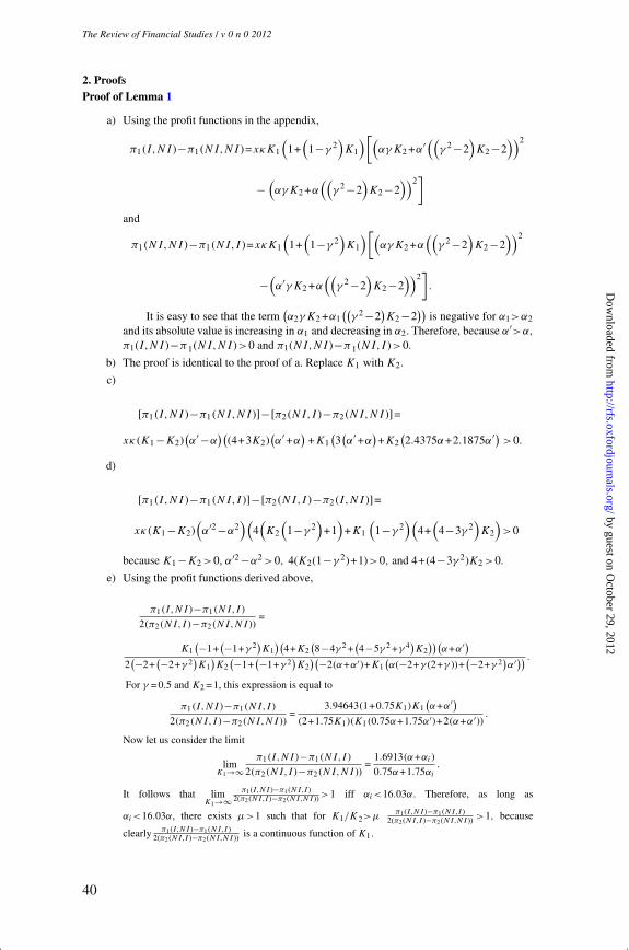
[17:53 25/10/2012 OEP-hhs109.tex] Page: 40 1–45


2. ProofsProof of Lemma 1

a) Using the profit functions in the appendix,

π1 (I,NI )−π1 (NI,NI )=xκK1

(1+

(1−γ 2

)K1

)[(αγK2 +α′((

γ 2 −2)K2 −2

))2

−(αγK2 +α

((γ 2 −2

)K2 −2

))2]

and

π1 (NI,NI )−π1 (NI,I )=xκK1

(1+

(1−γ 2

)K1

)[(αγK2 +α

((γ 2 −2

)K2 −2

))2

−(α′γK2 +α

((γ 2 −2

)K2 −2

))2].

It is easy to see that the term(α2γK2 +α1

((γ 2 −2

)K2 −2

))is negative for α1>α2

and its absolute value is increasing in α1 and decreasing in α2. Therefore, because α′>α,

π1(I,NI )−π1(NI,NI )>0 and π1(NI,NI )−π1(NI,I )>0.

b) The proof is identical to the proof of a. Replace K1 with K2.

c)

[π1 (I,NI )−π1 (NI,NI )]−[π2 (NI,I )−π2 (NI,NI )]=

xκ (K1 −K2)(α′ −α

)((4+3K2)

(α′ +α

)+K1

(3(α′ +α

)+K2

(2.4375α+2.1875α′) >0.

d)

[π1 (I,NI )−π1 (NI,I )]−[π2 (NI,I )−π2 (I,NI )]=

xκ (K1 −K2)(α′2 −α2

)(4(K2

(1−γ 2

)+1

)+K1

(1−γ 2

)(4+

(4−3γ 2

)K2

)>0

because K1 −K2 >0, α′2 −α2 >0, 4(K2(1−γ 2)+1)>0, and 4+(4−3γ 2)K2 >0.

e) Using the profit functions derived above,

π1 (I,NI )−π1 (NI,I )

2(π2 (NI,I )−π2 (NI,NI ))=

K1(−1+

(−1+γ 2)K1

)(4+K2

(8−4γ 2 +

(4−5γ 2 +γ 4

)K2

))(α+α′)

2(−2+

(−2+γ 2)K1

)K2

(−1+(−1+γ 2

)K2

)(−2(α+α′)+K1(α(−2+γ (2+γ ))+

(−2+γ 2)α′)) .

For γ =0.5 and K2 =1, this expression is equal to

π1 (I,NI )−π1 (NI,I )

2(π2 (NI,I )−π2 (NI,NI ))=

3.94643(1+0.75K1)K1(α+α′)

(2+1.75K1)(K1 (0.75α+1.75α′)+2(α+α′)) .

Now let us consider the limit

limK1→∞

π1 (I,NI )−π1 (NI,I )

2(π2 (NI,I )−π2 (NI,NI ))=

1.6913(α+αi )

0.75α+1.75αi

.

It follows that limK1→∞

π1(I,NI )−π1(NI,I )2(π2(NI,I )−π2(NI,NI )) >1 iff αi<16.03α. Therefore, as long as

αi<16.03α, there exists μ>1 such that for K1/K2>μπ1(I,NI )−π1(NI,I )

2(π2(NI,I )−π2(NI,NI )) >1, because

clearly π1(I,NI )−π1(NI,I )2(π2(NI,I )−π2(NI,NI )) is a continuous function of K1.

40



ownloaded from


[17:53 25/10/2012 OEP-hhs109.tex] Page: 41 1–45


f) If γ =0.5 and K2 =1, then

2(π1 (I,NI )−π1 (NI,NI ))

π2 (NI,I )−π2 (I,NI )=

0.203175(4/3+K1)(21.0938α2

i −5.625ααi −15.4688α2)

(k1 +8/9)(k1 +1.6)(α2

i −α2) .

The limit of this expression for K1 →∞ is4.2856α2

i −1.1429ααi−3.1419α2

α2i −α2 >1for αi >α.

g) Consider the quantity π2(NI,I )−2π2(NI,NI )+π2(I,NI )=

xκK2(1+(1−γ 2)K2)[((α′−α)((γ 2−2)K1−2)2+γK2)]>0, where

κ =[4−2

(−2+γ 2

)K2 +K1

(γ 4K2 +4(1+K2)−γ 2(2+5K2)

)]−2.

�

Proof of Proposition 2

1) Let V1,2(A1,A2) be the value of the big (small) firm as a function of its own actions andthose of its competitor. Then, for x <x1,

V1(I,NI )=π1(I,NI )x−RD; V1(NI,NI )=π1(NI,NI )x.

It follows that for x <x1 V1(I,NI )<V1(NI,NI ). It also follows from Lemma 1 c) thatV2(NI,I )<V2(NI,NI ). Then, (NI,NI ) is the Nash equilibrium for x <x1, while neither(I,NI ) nor (NI,I ) is an equilibrium in this region. Furthermore, the value of the small firmif both firms invest is V2(I,I )=0.5[(π2(I,NI )+π2(I,NI )]x−RD, while V2(I,NI )=π2(I,NI )x, so x <x3 (I,I ) is not a Nash equilibrium. Lemma 1 f) establishes that x1 <x3;therefore, the only Nash equilibrium for x <x1 is (NI,NI ).

2) If x1 <x <x3, then (I,NI ) is a Nash equilibrium. Indeed, V1(NI,NI )<V1(I,NI ) forx1 <x, and V2(I,I )<V2(I,NI ) for x <x3. It follows that neither (I,I ) nor (NI,NI ) isan equilibrium. (NI,I ) is not an equilibrium either as long as condition e) of Lemma 1holds: it is straightforward to see that for x >x4V1(NI,I )<V1(I,I ).Thus, (I,NI ) is theonly Nash equilibrium in this region.

3) Finally, for x >x3 it becomes optimal for the small firm to invest as well. In this region,

V2(I,I )=(π2(NI,I )+π2(I,NI ))x

2−RD; V2(I,NI )=π2(I,NI )x,

so V2(I,I )>V2(I,NI ). On the other hand, V1(I,I )>V1(NI,I ) for x >x3 >x4

(Lemma 1 d) establishes that x3 >x4). It is also straightforward to see that (NI,NI )is not an equilibrium for x >x1. Lemma 1 f) ensures that x3 >x1. Therefore, (I,I ) is theonly Nash equilibrium in this region. �

Proof of Proposition 3Note that a merger always results in increased market power, so if Im =0, a merger always occurs.Also note that condition π2(NI,I )−π2(NI,NI )>π2(NI,NI )−π2(I,NI ) implies that x2 <x3.

Then, for x <x1m,

V1(I,NI )= (πm(I )−π2(I,NI ))x−RD; V1(NI,NI )= (πm(NI )−π2(NI,NI ))x.

Therefore, V1(I,NI )<V1(NI,NI ). On the other hand, πm(I )−πm(NI )>0, and therefore

πm(I )−πm(NI )+π2(NI,NI )−π2(I,NI )>π2(NI,NI )−π2(I,NI ).

It follows that x1m <x2 and for x <x1mV2(NI,NI )>V2(NI,I ). It follows that (NI,NI ) is aNash equilibrium, while neither (I,NI ) nor (NI,I ) is an equilibrium. Furthermore, because

41



ownloaded from


[17:53 25/10/2012 OEP-hhs109.tex] Page: 42 1–45


πm(I )−πm(NI )>π1(I,NI )−π1(NI,NI ), it follows that x1m <x1 <x3 (Lemma 1 f), andV2(I,NI )>V2(I,I ),so (I,I ) is not a Nash equilibrium.

For x1m <x <x2, the only Nash equilibrium is (I,NI ). Indeed, in this region V2(NI,NI )>V2(NI,I )>V2(I,I ) and the small firm never invests in this region, while the big firm invests asV1(I,NI )>V1(NI,NI ).

For x2 <x <x3, the following inequalities hold: V1(I,NI )>V1(NI,NI );V1(I,I )<V1(NI,I );V2(I,NI )>V2(I,I );V2(NI,I )>V2(NI,NI ).

The first inequality has been proven above for x >x1m. The second results from comparing thevalues of the big firm if it invests:

V1(I,I )=0.5(πm(I )−π2(I,NI ))x+0.5(πm(I )−π2(NI,I ))x−RD,

and if it does not:V1(NI,I )= (πm(I )−π2(NI,I ))x.

The third equation comes from comparing the values of the small firm if it invests: V2(I,I )=(π2(NI,I )−π2(I,NI ))x

2 −RD and if it does not: V2(I,NI )=π2(I,NI )x, the fourth equation has beenproven above.

Therefore, both (I,NI ) and (NI,I ) are Nash equilibria. In addition, there is a mixed-strategyequilibrium in which the big firm invests with probability φ1 and the small firm invests withprobability φ2.To find these probabilities, note that in this equilibrium both firms must be indifferentbetween investing and not. Therefore,

φ1V2(I,I )+(1−φ1)V2(NI,I )=φ1V2(I,NI )+(1−φ1)V2(NI,NI )

andφ2V1(I,I )+(1−φ2)V1(I,NI )=φ2V1(NI,I )+(1−φ2)V1(NI,NI )

or

φ1 =V2(NI,NI )−V2(NI,I )

V2(I,I )−V2(NI,I )−V2(I,NI )+V2(NI,NI )

and

φ2 =V1(NI,NI )−V1(I,NI )

V1(I,I )−V1(NI,I )−V1(I,NI )+V1(NI,NI ).

It is straightforward to see that 0<φ1 <1 and 0<φ2 <1 so the mixed-strategy equilibrium alwaysexists.

Finally, for x >x3,V1(I,I )>V1(NI,I ) and V2(I,NI )<V2(I,I ); therefore, (I,I ) is the onlyNash equilibrium. �

Proof of Proposition 5First consider the case x1η <x2η. Consider the values of the big firm:

V1(I,NI )=π1(I,NI )x+(1−η)(πm(I )−π1(I,NI )−π2(I,NI ))x−RD

andV1(NI,NI )=π1(NI,NI )x+(1−η)(πm(NI )−π1(NI,NI )−π2(NI,NI ))x.

It follows that if x <x1η, then V1(NI,NI )>V1(I,NI ). Similarly, the values of the small firm are

V2(NI,I )=π2(NI,I )x+η(πm(I )−π1(NI,I )−π2(NI,I ))x−RD,

V2(NI,NI )=π2(NI,NI )x+η(πm(NI )−π1(NI,NI )−π2(NI,NI ))x.

So, for x <x1η <x2η , V2(NI,NI )>V2(NI,I ). Finally, because x1η <x2η <x3η,V2(I,I )<V2(I,NI ), neither (NI,I ) nor (I,NI ) nor (I,I ) is a Nash equilibrium.

42



ownloaded from


[17:53 25/10/2012 OEP-hhs109.tex] Page: 43 1–45


If x1η <x <x2η it can be easily verified that V2(I,NI )>V2(I,I ), V1(I,NI )>V1(NI,NI ), andV2(NI,I )<V2(NI,NI ), so (I,NI ) is the only equilibrium in this region. The proof of equilibriumstrategies for x >x2η follows exactly the proof of Proposition 3.

Now consider the case x1η >x2η. Clearly (NI,NI ) is the only Nash equilibrium if x <x2η.

If x2η <x <x1η, it is easy to verify that V1(NI,NI )>V1(I,NI ), V2(NI,NI )<V2(NI,I ), andV2(I,I )<V2(I,NI ). It follows that the only Nash equilibrium in this region is (NI,I ). The restof the proof follows closely the proof of Proposition 3. �

References

Aghion, P., N. Bloom, R. Blundell, R. Griffin, and P. Howitt. 2002. Competition and innovation: An invertedU-shaped relationship. Working Paper, Harvard University.

Aghion, P., C. Harris, P. Howitt, and J. Vickers. 2001. Competition, imitation, and growth with step-by-stepinnovation. Review of Economic Studies 68:467–92.

Aghion, P., P. Askenazy, N. Berman, G. Cette, and L. Eymard. 2008. Credit constraints and the cyclicality ofR&D investment: Evidence from France. Working Paper, Harvard University.

Ambrose, B., and W. Megginson. 1992. The role of asset structure, ownership structure, and takeover defensesin determining acquisition likelihood. Journal of Financial and Quantitative Analysis 27:575–89.

Atanassov, J. 2009. Do hostile takeovers stifle innovation? Evidence from antitakeover legislation and corporatepatenting. Working Paper, University of Oregon.

Baily, M., and H. Gersbach. 1995. Efficiency in manufacturing and the need for global competition. BrookingsPapers on Economic Activity: Macroeconomics 307–47.

Barlevy, G. 2007. On the cyclicality of research and development. American Economic Review 97:1131–64.

Bena, J., and K. Li. 2012. Corporate innovations and mergers and acquisitions. Working Paper, University ofBritish Columbia.

Bernile, G., E. Lyandres, and A. Zhdanov. 2012. A theory of strategic mergers. Review of Finance 16:517–75.

Bloomberg. 2008. Innovation through acquisition. February 29.

Blundell, R., R. Griffin, and J. Van Reenen. 1999. Market share, market value, and innovation in a panel ofBritish manufacturing firms. Review of Economic Studies 66:529–54.

Chemmanur, T., and X. Tian. 2010. Do anti-takeover provisions spur corporate innovation? Working Paper,Boston College.

Dasgupta, P., and J. Stiglitz. 1980. Industrial structure and the nature of innovative activity. Economic Journal90:266–93.

Edmans, A., I. Goldstein, and W. Jiang. 2012. The real effects of financial markets: The impact of prices ontakeovers. Journal of Finance 67:933–71.

Eisfeldt,A., andA. Rampini. 2006. Capital reallocation and liquidity. Journal of Monetary Economics 53:369–99.

Ferreira, M., M. Massa, and P. Matos. 2010. Shareholders at the gate? Institutional investors and cross-bordermergers and acquisitions. Review of Financial Studies 23:601–44.

Forbes. 2005. Does innovation through acquisition work? November 8.

Forbes. 2008. Art of acquiring growth. January 4.

Fulghieri, P., and M. Sevilir. 2009. Organization and financing of innovation, and the choice between corporateand independent venture capital. Journal of Financial and Quantitative Analysis 44:1291–321.

Fulghieri, P., and M. Sevilir. 2011. Mergers, spin-offs, and employee incentives. Review of Financial Studies24:2207–41.

43



ownloaded from


[17:53 25/10/2012 OEP-hhs109.tex] Page: 44 1–45


Gaudet, G., and S. Salant. 1992. Towards a theory of horizontal mergers. In The New Industrial Economics, eds.G. Norman and M. La Manna. Brookfield, VT: Edward Elgar.

Hall, B. H. 1999. Mergers and R&D revisited. Working Paper, University of California at Berkeley.

Harford, J. 2005. What drives merger waves. Journal of Financial Economics 77:529–60.

Hoberg, G., and G. Phillips. 2010a. Real and financial industry booms and busts. Journal of Finance 65:45–86.

—–. 2010b. Product market synergies and competition in mergers and acquisitions: A text-based analysis. Reviewof Financial Studies 23:3773–811.

—–. 2011. Dynamic product-based industry classifications and endogenous product differentiation. WorkingPaper, University of Maryland.

Jovanovic, B., and P. L. Rousseau. 2002. The Q-theory of mergers. American Economic Review 92:198–204.

Lambrecht, B. 2004. The timing and terms of takeovers motivated by economies of scale. Journal of FinancialEconomics 72:41–62.

Lown, C., D. Morgan, and S. Rohatgi. 2000. Listening to loan officers: Commercial credit standards, lending,and output. In Federal Reserve Bank of New York Economic Policy Review.

Maksimovic, V., and G. Phillips. 2001. The market for corporate assets: Who engages in mergers and asset salesand are there efficiency gains? Journal of Finance 56:2019–65.

—–. 2008. The industry life-cycle, acquisitions, and investment: Does firm organization matter? Journal ofFinance 63:629–64.

Maksimovic, V., G. Phillips, and L. Yang. Forthcoming. Public and private merger waves. Journal of Finance.

Mitchell, M., and H. Mulherin. 1996. The impact of industry shocks on takeover and restructuring activity.Journal of Financial Economics 41:193–229.

Morck, R., A. Shleifer, and R. W. Vishny. 1990. Do managerial objectives drive bad acquisitions? Journal ofFinance 45:31–48.

Morellec, E., and A. Zhdanov. 2005. The dynamics of mergers and acquisitions. Journal of Financial Economics77:649–72.

Ortiz-Molina, H., and G. Phillips. Forthcoming. Real asset illiquidity and the cost of capital. Journal of Financialand Quantitative Analysis.

Pastor, L., and P. Veronesi. 2009. Technological revolutions and stock prices. American Economic Review99:1451–63.

Rhodes-Kropf, M., and S. Viswanathan. 2004. Market valuation and merger waves. Journal of Finance 59:2685–718.

Rhodes-Kropf, M., D. Robinson, and S. Viswanathan. 2005. Valuation waves and merger activity: The empiricalevidence. Journal of Financial Economics 77:561–603.

Rhodes-Kropf, M., and D. Robinson. 2008. The market for mergers and the boundaries of the firm. Journal ofFinance 63:1169–211.

Salant, S., S. Switzer, and R. Reynolds. 1983. Losses from horizontal merger: The effects of an exogenous changein industry structure on Cournot-Nash equilibrium. Quarterly Journal of Economics 98:185–199.

Nickell, S. J. 1996. Competition and corporate performance. Journal of Political Economy 104:724–46.

Schlingemann, F. P., R. M. Stulz, and R. A. Walkling. 2002. Divestitures and the liquidity of the market forcorporate assets Journal of Financial Economics 64:117–44.

Seru, A. Forthcoming. Firm boundaries matter: Evidence from conglomerates and R&D activity. Journal ofFinancial Economics.

44



ownloaded from


[17:53 25/10/2012 OEP-hhs109.tex] Page: 45 1–45


Shleifer, A., and R. Vishny. 1992. Liquidation values and debt capacity: A market equilibrium approach. Journalof Finance 47:1343–66.

Vives, X. 2000. Oligopoly pricing—old ideas and new tools. Cambridge, MA: MIT Press.

—–. 2008. Innovation and competitive pressure. Journal of Industrial Economics 56:419–69.

Zhou, W. 2008. Endogenous horizontal mergers under cost uncertainty. International Journal of IndustrialOrganization 26:903–12.

45



ownloaded from


Documents

R&D and the Incentives from Merger and …faculty.tuck.dartmouth.edu/.../gordon-phillips/rd_acquisitions.pdfR&D and the Incentives from Merger and AcquisitionActivity ... R&D and the