Embed Size (px)
Citation preview
Mathematical Programming Computation manuscript No.(will be inserted by the editor)
RBFOpt: an open-source library for black-boxoptimization with costly function evaluations
Alberto Costa · Giacomo Nannicini
Received: date / Accepted: date
Abstract We consider the problem of optimizing an unknown function givenas an oracle over a mixed-integer set. We assume that the oracle is expen-sive to evaluate, so that estimating partial derivatives by finite differences isimpractical. In the literature, this is typically called a black-box optimizationproblem with costly evaluation. Our approach is based on the Radial BasisFunction method originally proposed by Gutmann (2001), which builds anditeratively refines a surrogate model of the unknown objective function. Thetwo main methodological contributions of this paper are an approach to exploita noisy but less expensive oracle to accelerate convergence to the optimum ofthe exact oracle, and the introduction of an automatic model selection phaseduring the optimization process. Numerical experiments show that these con-tributions significantly improve the performance of the algorithm on a test setof continuous and mixed-integer nonlinear unconstrained problems taken fromthe literature. Our implementation is open-source and free for non-commercialacademic use.
Keywords Black-box optimization · Derivative free optimization · Globaloptimization · Radial basis function · Open-source software · Mixed-integernonlinear programming
A. CostaSingapore University of Technology and DesignE-mail: [email protected]
G. NanniciniSingapore University of Technology and DesignE-mail: [email protected]
2 Alberto Costa, Giacomo Nannicini
1 Introduction
In this paper, we address a problem cast in the following form:
min f(x)x ∈ [xL, xU ]x ∈ Zq × Rn−q,
(1)
where f : Rn → R, xL, xU ∈ Rn are vectors of lower and upper bounds on thedecision variables, and q ≤ n. We assume that f is continuous with respectto all variables, even though some of the variables are restricted to take onlyon integer values. Furthermore, we assume that the analytical expression forf is unknown and function values are only available through an oracle that isexpensive to evaluate, e.g. a time-consuming simulation. In the literature, thisis typically called a black-box optimization problem with costly evaluation.
This problem class finds many applications. Our work originated from aproject in architectural design where we faced the following problem (see also[9]). During the design phase, a building can be described by a parametricmodel and the parameters are the decision variables, that can be continuousor discrete. Lighting and heating simulation software can be used to studyenergy profiles of buildings, simulating sun exposure over a prescribed periodof time. This information can be used to determine a performance measure,i.e. an objective function, but the analytical expression is not available due tothe complexity of the simulations. The goal is to optimize this function to finda good parameterization of the parametric model of the building. However,each run of the simulation software usually takes considerable time: up toseveral hours. Thus, we want to optimize the objective function within a smallbudget of function evaluations to keep computing times under control. Otherapplications of this approach can be found in engineering disciplines wherethe simulation relies on the solution of a system of PDEs, for example inthe context of performance optimization for complex physical devices such asengines, see e.g. [2,18].
There is a very large stream of literature on black-box optimization ingeneral, also called derivative-free optimization (sometimes generating confu-sion). Numerous methods have been proposed, and the choice of a particularmethod should depend on the number of function evaluations allowed, the di-mension of the problem, and its structural properties. Heuristic approaches arevery common thanks to their simplicity, for example scatter search, simulatedannealing and evolutionary algorithms; see [13,12] for an overview. However,these methods are not specifically tailored for the setting of this paper andoften require a large number of function evaluations, as has been noted by [15,29] among others. In general, methods that do not take advantage of the in-herent smoothness of the objective function may take a long time to converge[6]. Unfortunately, because of the assumption of expensive function evaluation,estimating partial derivatives by finite differences is impractical and often hasprohibitive computational cost. A commonly used approach in this contextis that of building an approximation model of f , also called response surface
A library for black-box optimization 3
or surrogate model. Examples of this approach are the Radial Basis Function(RBF) method of [15] (see also [27]), the stochastic RBF method [29], andthe kriging-based Efficient Global Optimization method (EGO) of [23]. Thesurrogate model constructed by these methods is a global model that usesall available information on f , as opposed to methods that only build a localmodel such as trust-region based methods [6,7]. Other methods for black-boxoptimization rely on direct search, i.e., they do not build a surrogate model ofthe objective function. An overview of direct search methods can be found in[24], and a comprehensive treatment is given in [7]. We refer the reader to [31]and the references therein for a very recent survey on black-box methods andan extensive computational evaluation.
In this paper we focus on problems that are nonconvex, relatively small-dimensional, and for which only a small number of function evaluations isallowed. For this type of problems, algorithms based on a surrogate modelare typically considered among the most effective. In particular, empirical ev-idence [20] suggests that the RBF method is more effective on engineeringproblems, despite the appealing theoretical properties of other methodologiessuch as EGO. Besides this empirical evidence, there are three additional rea-sons that make a surrogate model method more appealing than direct searchin our context. The first reason is that looking for alternative optima, or atleast a set of good solutions, is easier if we can rely on a surrogate model. Thesecond reason is that it is intuitively easier to “warm-start” such a methodin a context where each function evaluation (i.e. simulation) produces somedata that allows for fast recomputation of different but related objective func-tions, because the model of these new objective functions can be quickly built.The third reason is that the surrogate model can sometimes be used to allowthe fast (potentially inaccurate) exploration of the objective function aroundthe optimum: we study this possibility in Section 5.7. These properties areimportant for our motivating application from a practical perspective, whichexplains our choice.
In this paper, we review the RBF method and present some extensionsaimed at improving its practical performance. Our most significant contribu-tions to the class of RBF methods are a fast procedure for automatic modelselection, and an approach to accelerate convergence in case we have access toan additional oracle that returns noisy function values (i.e. affected by error)but is less expensive to evaluate than the exact oracle for f . These contribu-tions could be adapted to other surrogate model based methods and shouldtherefore be considered of general interest, rather than specific for the RBFmethod. Our implementation of the method is an open-source library calledRBFOpt, and we show that it is competitive with state-of-the-art commercialsoftware on a set of test problems taken from the literature. In particular, thetwo main contributions of these paper significantly decrease the number offunction evaluations for global convergence on our test set. Furthermore, weshow that on our test set, the proposed methodology for automatic model se-lection yields a measure of model quality that is helpful in deciding whether or
4 Alberto Costa, Giacomo Nannicini
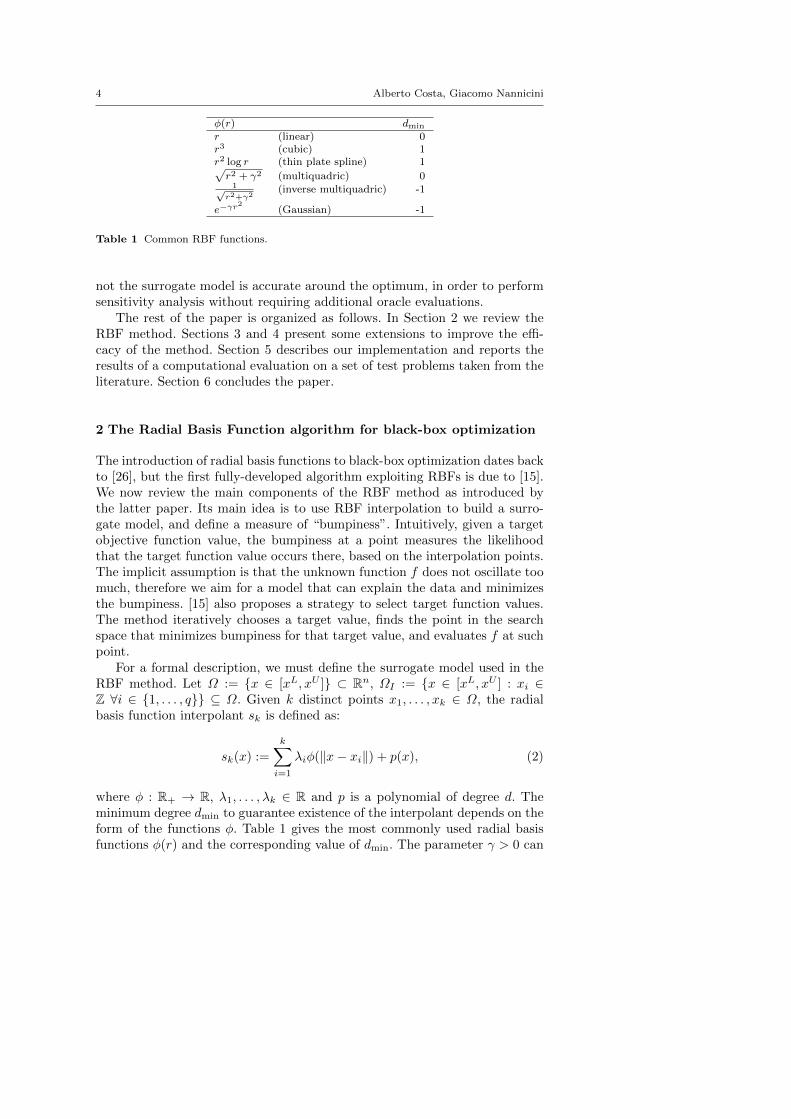
φ(r) dmin
r (linear) 0r3 (cubic) 1r2 log r (thin plate spline) 1√r2 + γ2 (multiquadric) 01√
r2+γ2(inverse multiquadric) -1
e−γr2
(Gaussian) -1
Table 1 Common RBF functions.
not the surrogate model is accurate around the optimum, in order to performsensitivity analysis without requiring additional oracle evaluations.
The rest of the paper is organized as follows. In Section 2 we review theRBF method. Sections 3 and 4 present some extensions to improve the effi-cacy of the method. Section 5 describes our implementation and reports theresults of a computational evaluation on a set of test problems taken from theliterature. Section 6 concludes the paper.
2 The Radial Basis Function algorithm for black-box optimization
The introduction of radial basis functions to black-box optimization dates backto [26], but the first fully-developed algorithm exploiting RBFs is due to [15].We now review the main components of the RBF method as introduced bythe latter paper. Its main idea is to use RBF interpolation to build a surro-gate model, and define a measure of “bumpiness”. Intuitively, given a targetobjective function value, the bumpiness at a point measures the likelihoodthat the target function value occurs there, based on the interpolation points.The implicit assumption is that the unknown function f does not oscillate toomuch, therefore we aim for a model that can explain the data and minimizesthe bumpiness. [15] also proposes a strategy to select target function values.The method iteratively chooses a target value, finds the point in the searchspace that minimizes bumpiness for that target value, and evaluates f at suchpoint.
For a formal description, we must define the surrogate model used in theRBF method. Let Ω := x ∈ [xL, xU ] ⊂ Rn, ΩI := x ∈ [xL, xU ] : xi ∈Z ∀i ∈ 1, . . . , q ⊆ Ω. Given k distinct points x1, . . . , xk ∈ Ω, the radialbasis function interpolant sk is defined as:
sk(x) :=
k∑i=1
λiφ(‖x− xi‖) + p(x), (2)
where φ : R+ → R, λ1, . . . , λk ∈ R and p is a polynomial of degree d. Theminimum degree dmin to guarantee existence of the interpolant depends on theform of the functions φ. Table 1 gives the most commonly used radial basisfunctions φ(r) and the corresponding value of dmin. The parameter γ > 0 can
A library for black-box optimization 5
be used to change the shape of these functions (but it is usually set to 1).If φ(r) is cubic or thin plate spline, dmin = 1 and we obtain an interpolant
of the form:
sk(x) :=
k∑i=1
λiφ(‖x− xi‖) + hT(x1
), (3)
where h ∈ Rn+1. The values of λi, h can be determined by solving the followinglinear system: (
Φ PPT 0(n+1)×(n+1)
)(λh
)=
(F
0n+1
), (4)
with:
Φ = (φ(‖xi − xj‖))i,j=1,...,k , P =
xT1 1...
...xTk 1
, λ =
λ1...λk
, F =
f(x1)...
f(xk)
.
If rank(P ) = n+ 1, the system (4) is nonsingular [15].If φ(r) is linear or multiquadric, dmin = 0 and P is the all-one column
vector of dimension k, whereas in the inverse multiquadric and Gaussian case,dmin = −1 and P is removed from system (4). The dimensions of the zeromatrix and vector in (4) are adjusted accordingly.
Next, we define the measure of bumpiness σ. The motivation for the useof bumpiness comes from the theory of natural cubic spline interpolation indimension one (RBFs can be seen as its extension to multivariate functions).It is well known that the natural cubic spline interpolant whose parametersare found by solving a system as (4) (where n = 1 and φ(r) = r3) is thefunction which minimizes
∫R[g′′(x)]2 dx among all the functions g : R→ R such
that ∀i ∈ 1, . . . , k g(xi) = f(xi). Hence,∫R[g′′(x)]2dx is a good measure of
bumpiness. It is shown in [15] that in the case of RBF interpolants in dimensionn, this can be generalized to:
σ(sk) = (−1)dmin+1k∑i=1
λisk(xi) = (−1)dmin+1k∑i=1
k∑j=1
λiλjφ(‖xi − xj‖) =
= (−1)dmin+1λTΦλ.
(5)
Let us assume that after k function values f(x1), . . . , f(xk) are evaluated, wewant to find a point in ΩI where it is likely that the unknown function attainsa target value f∗k ∈ R (strategies for selecting f∗k will be discussed in thefollowing). Let sy be the RBF interpolant subject to the conditions:
sy(xi) = f(xi) ∀i ∈ 1, . . . , k (6)
sy(y) = f∗k . (7)
The assumption of the RBF method is that a likely location for the point ywith function value f∗k is the one that minimizes σ(sy). That is, we look for

6 Alberto Costa, Giacomo Nannicini
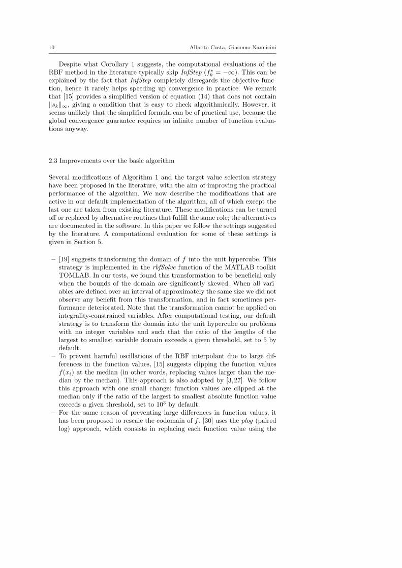
f ∗
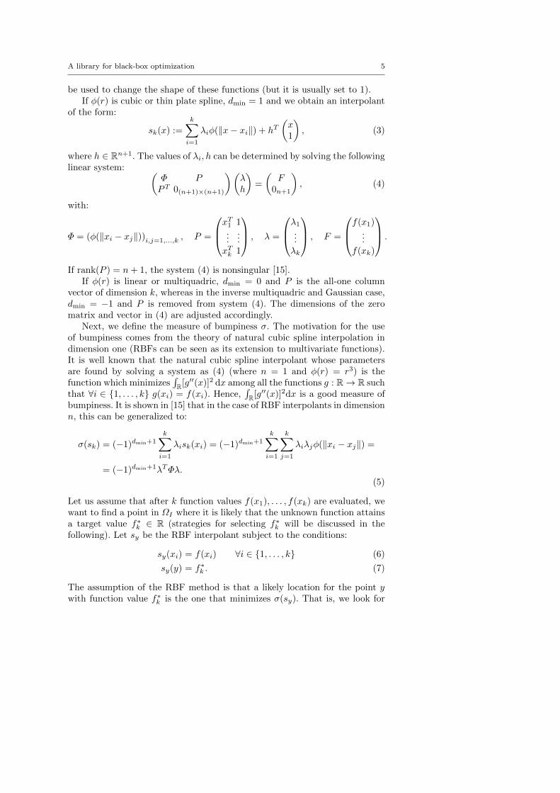
Fig. 1 An example with four interpolation points (circles) and a value of f∗k represented bythe horizontal dashed line. The RBF method assumes that it is more likely that a point withvalue f∗k is located at the diamond rather than the square, because the resulting interpolantis less bumpy.
the interpolant that is “the least bumpy”. A sketch of this idea is given inFigure 1.
Instead of computing the minimum of σ(sy) to find the least bumpy inter-polant, we define an equivalent optimization problem that is easier to solve.Let `k be the RBF interpolant to the points (xi, 0), ∀i ∈ 1, . . . , k and (y, 1).A solution to (6)-(7) can be rewritten as:
sy(x) = sk(x) + [f∗k − sk(y)]`k(x), x ∈ Rn,
which clearly interpolates at the desired points by definition of `k. Let µk(y) bethe coefficient corresponding to y of `k. µk(y) can be computed by extendingthe linear system (4), which becomes [15]: Φ u(y) P
u(y)T φ(0) π(y)T
PT π(y) 0
α(y)µk(y)b(y)
=
0k
10n+1
, (8)
where u(y) = (φ(‖y − x1‖), . . . , φ(‖y − xk‖))T and π(y) is(yT 1
)when dmin =
1, 1 when dmin = 0 and it is not used when dmin = −1. With algebraicmanipulations (see [15,27]) we can obtain from the system (8) the followingexpression for µk(y):
µk(y) =1
φ(0)− (u(y) π(y))T
(Φ PPT 0
)−1(u(y) π(y))
. (9)
A way of storing the factorization of Φ to speed up the computation of µk(y)is described in [3].
It can be shown [15] that computing the minimum of σ(sy) over y ∈ Rn isequivalent to minimizing the utility function:
gk(y) = (−1)dmin+1µk(y)[sk(y)− f∗k ]2, y ∈ Ω \ x1, . . . , xk.
A library for black-box optimization 7
Unfortunately gk and µk are not defined at x1, . . . , xk, and limx→xi µk(x) =∞, ∀i ∈ 1, . . . , k. To avoid numerical troubles, [15] suggests maximizing thefollowing function:
hk(x) =
1
gk(x)if x 6∈ x1, . . . , xk
0 otherwise,(10)
which is differentiable everywhere on Ω.We now have all the necessary ingredients to describe the RBF algorithm,
first introduced in [15]. We remark that q = 0 in the framework of [15], i.e.there are no integer variables. An extension to q > 0 is given in [20], andour exposition below follows the latter paper. The original algorithm can berecovered by substituting Ω for ΩI .
– Initial step: Choose linearly independent x1, . . . , xn ∈ ΩI using an ini-tialization strategy. Set k ← n. Compute the RBF sk that minimizes σ(sk)subject to the interpolation conditions:
sk(xi) = f(xi) ∀i ∈ 1, . . . , k.
– Iteration step: Repeat the following steps.– Choose a target value f∗k ∈ [−∞,minx∈ΩI
sk(x)](the choice f∗k = minx∈ΩI
sk(x) is admissible only if f∗k 6= f(xi) ∀i ∈1, . . . , k).
– Computexk+1 = arg max
x∈ΩI
hk(x), (11)
where h(x) is defined as in (10).– Evaluate f at xk+1 and compute the RBF interpolant sk+1 that mini-
mizes σ(sk+1) subject to sk+1(xi) = f(xi) ∀i ∈ 1, . . . , k + 1.– If we exceed a prescribed number of function evaluations, stop. Other-
wise, set k ← k + 1.
The pseudo-code of the RBF method is given in Algorithm 1.We still need to specify a strategy for choosing sample points in the Initial
step and the target value f∗k at each Iteration step. These will be the subjectof the next two sections. Afterwards, we discuss a number of modifications tothe basic algorithms that have been proposed in the literature and found tobe beneficial in practice.
2.1 Choice of the initial sample points
A natural choice for the initial sample points is to pick the 2n corner points ofthe box Ω, but this is reasonable only for small values of n. A commonly usedstrategy [15,19,20] for selecting the initial sample points is to choose n + 1corner points of the box Ω, and the central point of Ω, but this could prioritizethe exploration in a part of the domain. [20] chooses xL and xL+eTi (xUi −xLi )
8 Alberto Costa, Giacomo Nannicini
input : oracle for f , domain [xL, xU ], maximum # evaluations nmax
output: best solution found within nmax evaluations
evaluate f at k0 starting points x1 . . . xk0 with n+ 1 ≤ k0 ≤ nmax;i←− arg minf(xi), ∀i ∈ 1, . . . , k0;(x∗, f∗)←− (xi, f(xi));k ←− k0;while k < nmax do
compute the interpolant sk(x) using the k points evaluated so far;choose a target value f∗k and select the next evaluation point xk+1;evaluate f(xk+1) through the oracle;if f(xk+1) < f∗ then
x∗ ←− xk+1;f∗ ←− f(xk+1);
endk ←− k + 1;
endreturn (x∗, f∗)
Algorithm 1: Pseudo-code of the RBF method.
for i = 1, . . . , n as initial corner points, where ei is the i-th vector of thestandard orthonormal basis. Note that these points may not be feasible forΩI . We can round the integer components of the points to achieve feasibility.
Another commonly used strategy is to use a Latin Hypercube experimen-tal design, typically chosen among some randomly generated Latin Hypercubedesigns according to a maximum minimum distance or a minimum maximumcorrelation criterion. Again, points sampled this way may not be feasible forΩI , and we apply rounding. Note that some of the rounded points may coin-cide, in which case additional sample points have to be constructed because werequire linear independence. This is our default strategy in the computationalexperiments.
[20] considers the case where some explicit constraints are given in theproblem formulation and added to ΩI , and suggests sampling more pointsthan strictly necessary (i.e. > n+ 1), and picking the first n+ 1 feasible ones.In practice, feasibility for ΩI should not be too difficult to obtain, otherwisesolving the initial problem (1) is hopeless. In our setting, where ΩI is a boxwith integrality on some variables, the simple rounding strategy appears to besufficient for practical purposes.
2.2 Selection of the target value f∗k
To tackle the problem of selecting the target value f∗k at each Iteration step,we employ the technique proposed in [20], that generalizes [15], as describedbelow. Let y∗ := arg minx∈ΩI
sk(x), fmin := mini=1,...,k f(xi), and fmax :=maxi=1,...,k f(xi). In particular, we employ a cyclic strategy that picks targetvalues f∗k ∈ [−∞, sk(y∗)] according to the following sequence of length κ+ 2:
A library for black-box optimization 9
– Step −1 (InfStep): Choose f∗k = −∞. In this case the problem of findingxk+1 can be rewritten as:
xk+1 = arg maxx∈ΩI
1
(−1)dmin+1µk(x).
This is an exploration phase: the algorithm tries to improve the surrogatemodel in unknown parts of the domain.
– Step h ∈ 0, . . . , κ− 1 (Global search): Choose
f∗k = sk(y∗)− (1− h/κ)2(fmax − sk(y∗)). (12)
In this case, there is a balance between improving the model quality andfinding the minimum. Notice that if f∗k = sk(y∗), then
xk+1 = arg maxx∈ΩI
1
(−1)dmin+1sk(x). (13)
Hence, if (−1)dmin+1 = 1 there is not need to solve the problem, as xk+1 =y∗.
– Step κ (Local search): If sk(y∗) < fmin − 10−10|fmin| accept y∗ as the newsample point xk+1 without solving (11). Otherwise choose f∗k = fmin −10−2|fmin|. This is an exploitation phase: we try to find the best objectivefunction value based on the current surrogate model.
The choice of the target values is important for convergence of the method.In order to show ε-convergence to a global optimum for any continuous func-tion, it is necessary and sufficient [33] that the sequence of points (xk) gen-erated by the algorithm is dense in the projection of ΩI over Rn−q, i.e. thecontinuous variables, for every value of the integer variables in Zq ∩ ΩI . [15]considers the case where q = 0 and shows that (xk) is dense over Ω when φis linear, cubic or thin plate spline, if f∗ is “small enough” throughout theoptimization algorithm.
Theorem 1 [15] Let q = 0, φ(r) = r, φ(r) = r2 log r or φ(r) = r3. Further,choose the integer m such that 0 ≤ m ≤ n in the linear case, 1 ≤ m ≤ n + 1in the thin plate spline case, and 1 ≤ m ≤ n + 2 in the cubic case. Let (xk),k ∈ N be the sequence generated by Algorithm 1, and sk be the the RBFthat interpolates (xi, f(xi)), ∀i ∈ 1, . . . , k. Assume that, for infinitely manyk ∈ N, the choice of f∗k satisfies:
miny∈Ω
sk(y)− f∗k > τ∆ρ/2k ‖sk‖∞, (14)
where τ > 0, 0 ≤ ρ < dmin are constants, and ∆k := min1≤i≤k−1 ‖xk − xi‖.Then the sequence (xk) is dense in Ω.
Corollary 1 [15] Let f be continuous and the assumptions of Theorem 1 hold.Furthermore, assume that f∗k = −∞ for infinitely many k ∈ N. Then Algo-rithm 1 converges to a global optimum of f as k →∞.
10 Alberto Costa, Giacomo Nannicini
Despite what Corollary 1 suggests, the computational evaluations of theRBF method in the literature typically skip InfStep (f∗k = −∞). This can beexplained by the fact that InfStep completely disregards the objective func-tion, hence it rarely helps speeding up convergence in practice. We remarkthat [15] provides a simplified version of equation (14) that does not contain‖sk‖∞, giving a condition that is easy to check algorithmically. However, itseems unlikely that the simplified formula can be of practical use, because theglobal convergence guarantee requires an infinite number of function evalua-tions anyway.
2.3 Improvements over the basic algorithm
Several modifications of Algorithm 1 and the target value selection strategyhave been proposed in the literature, with the aim of improving the practicalperformance of the algorithm. We now describe the modifications that areactive in our default implementation of the algorithm, all of which except thelast one are taken from existing literature. These modifications can be turnedoff or replaced by alternative routines that fulfill the same role; the alternativesare documented in the software. In this paper we follow the settings suggestedby the literature. A computational evaluation for some of these settings isgiven in Section 5.
– [19] suggests transforming the domain of f into the unit hypercube. Thisstrategy is implemented in the rbfSolve function of the MATLAB toolkitTOMLAB. In our tests, we found this transformation to be beneficial onlywhen the bounds of the domain are significantly skewed. When all vari-ables are defined over an interval of approximately the same size we did notobserve any benefit from this transformation, and in fact sometimes per-formance deteriorated. Note that the transformation cannot be applied onintegrality-constrained variables. After computational testing, our defaultstrategy is to transform the domain into the unit hypercube on problemswith no integer variables and such that the ratio of the lengths of thelargest to smallest variable domain exceeds a given threshold, set to 5 bydefault.
– To prevent harmful oscillations of the RBF interpolant due to large dif-ferences in the function values, [15] suggests clipping the function valuesf(xi) at the median (in other words, replacing values larger than the me-dian by the median). This approach is also adopted by [3,27]. We followthis approach with one small change: function values are clipped at themedian only if the ratio of the largest to smallest absolute function valueexceeds a given threshold, set to 103 by default.
– For the same reason of preventing large differences in function values, ithas been proposed to rescale the codomain of f . [30] uses the plog (pairedlog) approach, which consists in replacing each function value using the
A library for black-box optimization 11
following transformation:
plog(x) =
log(1 + x) if x ≥ 0,
− log(1− x) if x < 0.
[20] replaces the values f(xi) > max(0, fmin)+105 with max(0, fmin)+105+log10(f(xi)−max(0, fmin) + 105). Our implementation offers the followingthree choices for function scaling:– off : we employ the original, unscaled function values;– log scaling: if fmin ≥ 1 we replace each f(xi) with log(f(xi)), otherwise
we replace it with log(f(xi) + 1 + |fmin|) (similar to [20]);
– affine scaling: we replace each f(xi) with f(xi)−fmin
fmax−fmin.
– In the Global search step, [15,27] replace fmax in equation (12) with a dy-namically chosen value f(xπ(α(k))), defined as follows. Let k0 be the numberof initial sampling points, h the index of the current Global search itera-tion as in Section 2.2, π a permutation of 1, . . . , k such that f(xπ(1)) ≤f(xπ(2)) ≤ · · · ≤ f(xπ(k)), and
α(k) =
k if h = 0
α(k − 1)−⌊k−k0κ
⌋otherwise.
As a result, fmax is used to define the target value f∗k only at the firststep (h = 0) of each Global search cycle. In subsequent steps, we pickprogressively lower values of f(xi), so as to stabilize search by avoiding toolarge differences between the minimum of the RBF interpolant, and thetarget value.
– If the initial sample points are chosen with a random strategy (for exam-ple, a Latin Hypercube design), whenever we detect that the algorithm isstalling, we apply a complete restart strategy [27, Sect. 5]. Restart strate-gies have been applied to numerous combinatorial optimization problems,such as satisfiability [14] and integer programming [1]. In the context ofthe RBF algorithm, the restart strategy as introduced in [27] works byrestarting the algorithm from scratch (including the generation of new ini-tial sample points) whenever the best known solution does not improve byat least a specified value (0.1% by default) after a given number of opti-mization cycles (5 by default). In our experience restarts tend to be moreuseful if the initial sample points are chosen according to a randomizedstrategy (otherwise the random number generator has impact only on thesolvers for the auxiliary problems).
– A known issue of the RBF method, explicitly pointed out in [27, Sect. 4],is that large values of h in Global search do not necessarily imply that thealgorithm is performing a “relatively local” search as intended. In fact, thenext iterate can be arbitrarily far from the currently known best point, andthis can severely hamper convergence on problems where the global mini-mum is in a steep valley. To alleviate this issue, [27, Sect. 4.3] proposes a“restricted global minimization of the bumpiness function”. The basic idea
12 Alberto Costa, Giacomo Nannicini
is to progressively restrict the search box around the best known solutionduring a Global search cycle. In particular, instead of solving (13) over ΩI ,we intersect ΩI with the box [miny∈ΩI
sk(y)− βk(xUxL),miny∈ΩIsk(y) +
βk(xUxL)], where βk = 0.5(1− h/κ) if (1− h/κ) ≤ 0.5, and βk = 1 other-wise (the numerical constants indicated are the values suggested by [27]).It is easy to verify that this restricts the global search to a box centered onthe global minimizer of the RBF interpolant: the box coincides with ΩI atthe beginning of every Global search cycle, but gets smaller as h increases.This turns out to be very beneficial on problems with steep global minima.
– A simple strategy that we found to be effective (see Section 5) is to repeatthe Local search step in case a Local search successfully improves the bestknown solution. In our experiments, it was not beneficial to perform Localsearch more than twice in a row, as this runs a high risk of focusing toomuch on a local minimum, forsaking global search.
3 Automatic model selection
One of the drawbacks of the RBF method is that there is no mechanism toassess model quality. There are many possible surrogate models depending onthe choice of the basis functions among those of Table 1, and it is difficult topredict a priori which one of these models would have the best performanceon a specific problem.
We propose an assessment of model quality using a cross validation scheme.This allows us to dynamically choose the surrogate model that appears to bethe most accurate for the problem at hand. Cross validation is a commonlyused model validation technique in statistics. Given a data set, cross validationconsists in using part of the data set to fit a model, and testing its quality onthe remaining part of the data set. The process is then iterated rotating theparts of the data set used for model fitting and for testing.
Let sk be our surrogate model for f based on k evaluation points x1, . . . , xk.We assume that the points are sorted by increasing function value: f(x1) ≤f(x2) ≤ · · · ≤ f(xk). We perform cross validation as follows. For j ∈ 1, . . . , k,we can fit a surrogate model sk,j to the points (xi, f(xi)) for i = 1, . . . , k, i 6= jand evaluate the performance of sk,j at (xj , f(xj)). In particular, we computethe value qk,j = |sk,j(xj)− f(xj)| to assess the predictive power of the model.We then average qk,j over j = 1, . . . , k to compute a model quality score. Thisapproach is known as leave-one-out cross validation in statistics.
We perform model selection at the beginning of every cycle of the searchstrategy to select f∗k , see Section 2.2. Our aim is to select the RBF model withthe best predictive power. Since the algorithm iterates between local searchand global search, we choose two different models: one for local search, one forglobal search. We achieve this goal by computing the average value q10% of qk,jfor j = 1, . . . , b0.1kc, and the average value q70% of qk,j for j = 1, . . . , b0.7kc,for a subset of the basis functions of Table 1. The rationale of our approachis that q10% is an estimate of how good a particular surrogate model is at
A library for black-box optimization 13
predicting function values for the points that have a low function value, whichare arguably the most important for local search. On the other hand, forglobal search it seems reasonable to choose a model that has good predictiveperformance on a larger range of function values, hence we use q70%. Thepoints with the highest function values are the farthest from the minimumand our assumption is that they can be disregarded.
The RBF model with the lowest value of q10% is employed in the subsequentoptimization cycle for the Local search step and the Global search step withh = κ − 1, while the RBF model with lowest value of q70% is employed forall the remaining steps. In our experiments, the RBF models that we considerare those with cubic, thin plate spline or multiquadric (with γ = 1) basisfunctions. We exclude the linear basis function because in our experience itsometimes leads to numerically unstable models, and its inclusion did not yielda noticeable performance increase in terms of model quality. It is possible toalso include different scaling parameters as described in Section 2.3 in theevaluation, but we did not pursue this possibility.
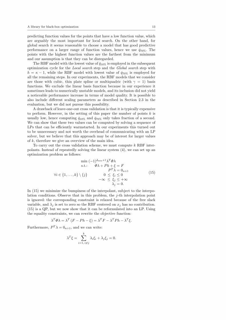
A drawback of leave-one-out cross validation is that it is typically expensiveto perform. However, in the setting of this paper the number of points k isusually low, hence computing q10% and q70% only takes fraction of a second.We can show that these two values can be computed by solving a sequence ofLPs that can be efficiently warmstarted. In our experiments this turned outto be unnecessary and not worth the overhead of communicating with an LPsolver, but we believe that this approach may be of interest for larger valuesof k, therefore we give an overview of the main idea.
To carry out the cross validation scheme, we must compute k RBF inter-polants. Instead of repeatedly solving the linear system (4), we can set up anoptimization problem as follows:
min (−1)dmin+1λTΦλs.t.: Φλ+ Ph+ ξ = F
PTλ = 0n+1
∀i ∈ 1, . . . , k \ j 0 ≤ ξi ≤ 0−∞ ≤ ξj ≤ +∞
λj = 0.
(15)
In (15) we minimize the bumpiness of the interpolant, subject to the interpo-lation conditions. Observe that in this problem, the j-th interpolation pointis ignored: the corresponding constraint is relaxed because of the free slackvariable, and λj is set to zero so the RBF centered on xj has no contribution.(15) is a QP, but we now show that it can be reformulated into an LP. Usingthe equality constraints, we can rewrite the objective function:
λTΦλ = λT (F − Ph− ξ) = λTF − λTPh− λT ξ.
Furthermore, PTλ = 0n+1, and we can write:
λT ξ =
k∑i=1, i 6=j
λiξi + λjξj = 0.
14 Alberto Costa, Giacomo Nannicini
This holds because λj = 0 and ξi = 0 ∀i 6= j. Hence the objective functionof (15) can be rewritten as λTF , and the problem can be reformulated as thefollowing LP:
min (−1)dmin+1λTFs.t.: Φλ+ Ph+ ξ = F
PTλ = 0n+1
∀i ∈ 1, . . . , k \ j 0 ≤ ξi ≤ 0−∞ ≤ ξj ≤ +∞
λj = 0.
(16)
Notice that changing the index j in (16) involves modifications of the variablebounds. Therefore, we can solve a sequence of LP problems of the form (16)with the dual simplex method.
4 The RBF method with a noisy oracle
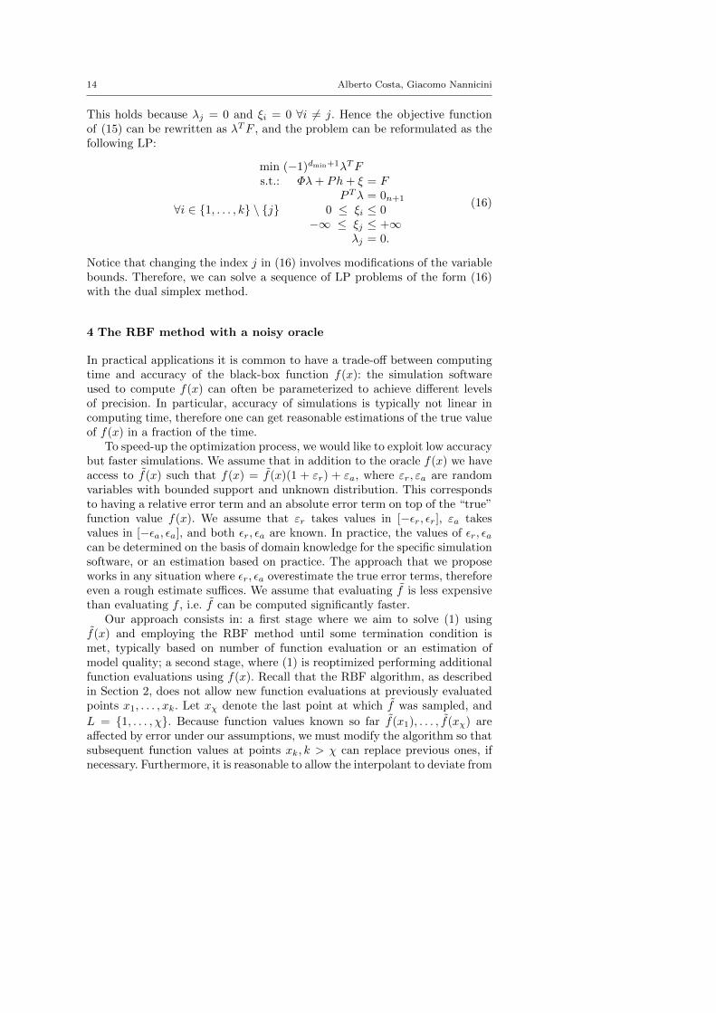
In practical applications it is common to have a trade-off between computingtime and accuracy of the black-box function f(x): the simulation softwareused to compute f(x) can often be parameterized to achieve different levelsof precision. In particular, accuracy of simulations is typically not linear incomputing time, therefore one can get reasonable estimations of the true valueof f(x) in a fraction of the time.
To speed-up the optimization process, we would like to exploit low accuracybut faster simulations. We assume that in addition to the oracle f(x) we haveaccess to f(x) such that f(x) = f(x)(1 + εr) + εa, where εr, εa are randomvariables with bounded support and unknown distribution. This correspondsto having a relative error term and an absolute error term on top of the “true”function value f(x). We assume that εr takes values in [−εr, εr], εa takesvalues in [−εa, εa], and both εr, εa are known. In practice, the values of εr, εacan be determined on the basis of domain knowledge for the specific simulationsoftware, or an estimation based on practice. The approach that we proposeworks in any situation where εr, εa overestimate the true error terms, thereforeeven a rough estimate suffices. We assume that evaluating f is less expensivethan evaluating f , i.e. f can be computed significantly faster.
Our approach consists in: a first stage where we aim to solve (1) usingf(x) and employing the RBF method until some termination condition ismet, typically based on number of function evaluation or an estimation ofmodel quality; a second stage, where (1) is reoptimized performing additionalfunction evaluations using f(x). Recall that the RBF algorithm, as describedin Section 2, does not allow new function evaluations at previously evaluatedpoints x1, . . . , xk. Let xχ denote the last point at which f was sampled, and
L = 1, . . . , χ. Because function values known so far f(x1), . . . , f(xχ) areaffected by error under our assumptions, we must modify the algorithm so thatsubsequent function values at points xk, k > χ can replace previous ones, ifnecessary. Furthermore, it is reasonable to allow the interpolant to deviate from

A library for black-box optimization 15
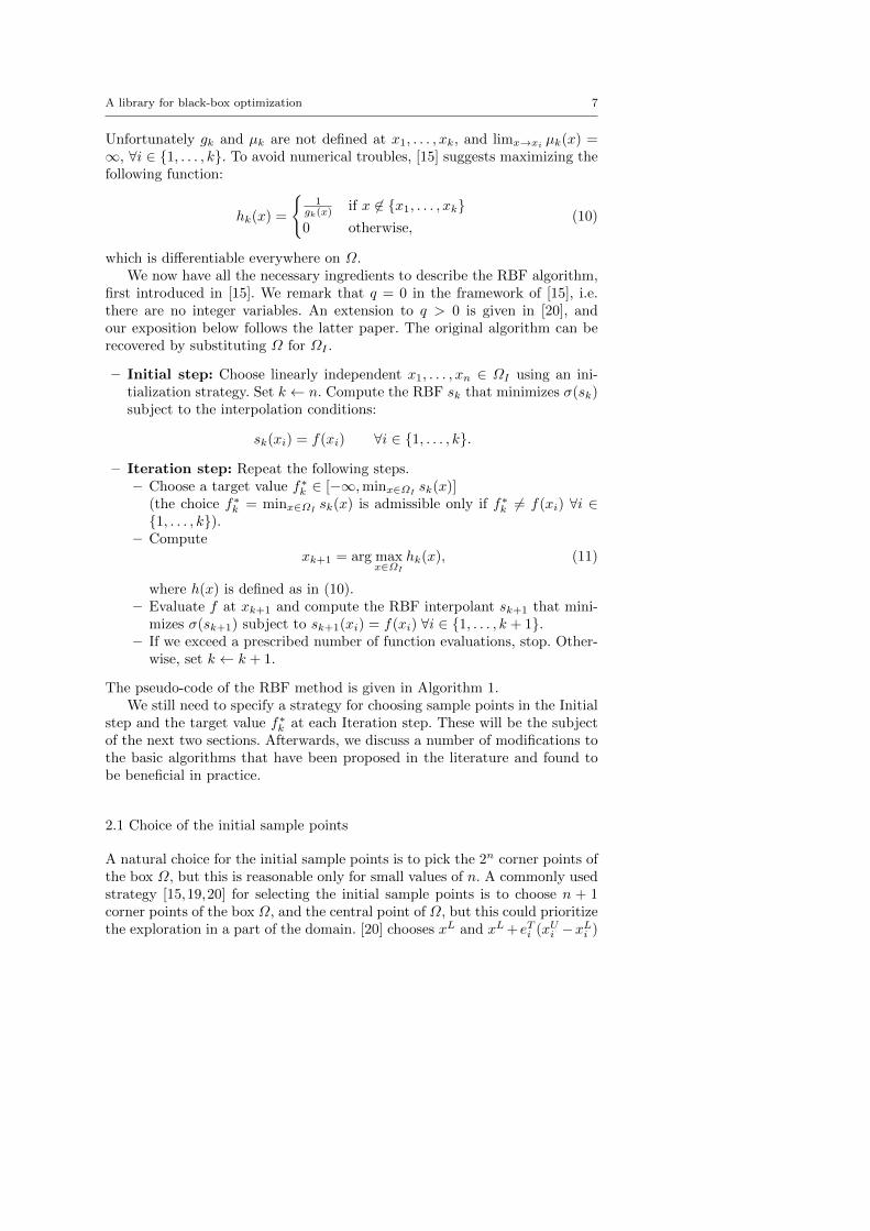
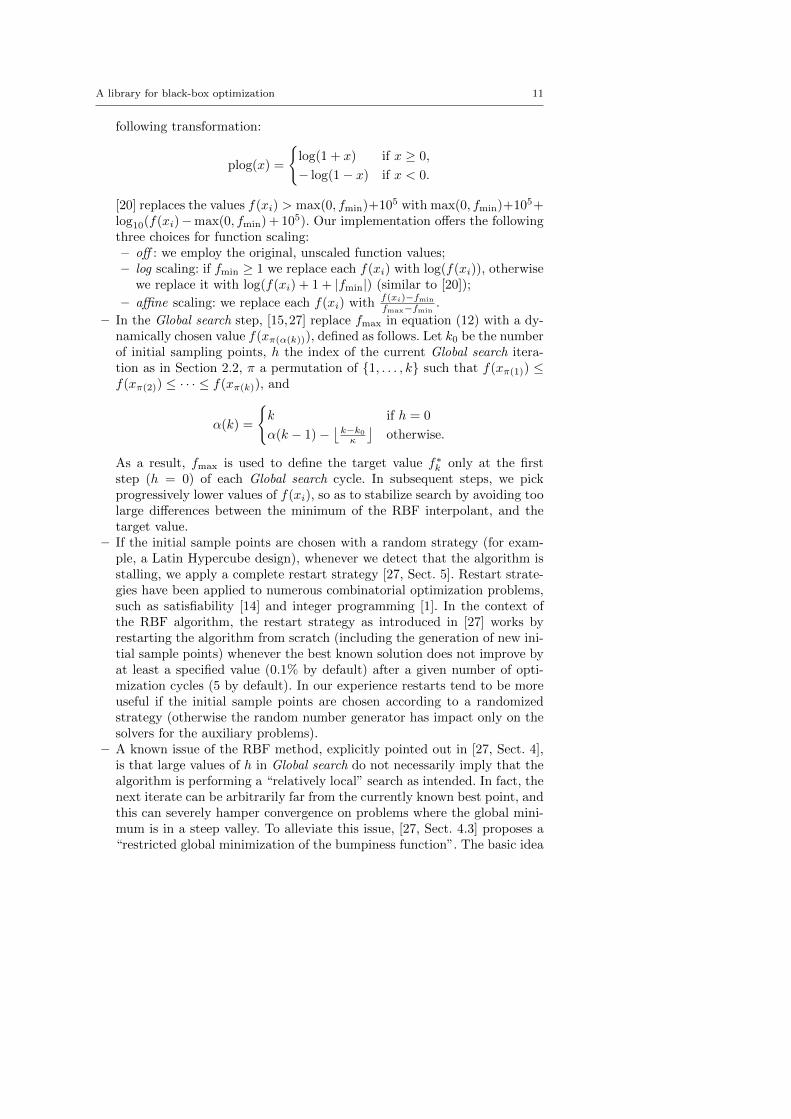
Fig. 2 Function evaluations affected by errors: the values returned by f are the circles. Thedashed line interpolates exactly at those points, the solid line is a less bumpy interpolant, andis still within the allowed error tolerances. Problem (17) would prefer the latter interpolant.
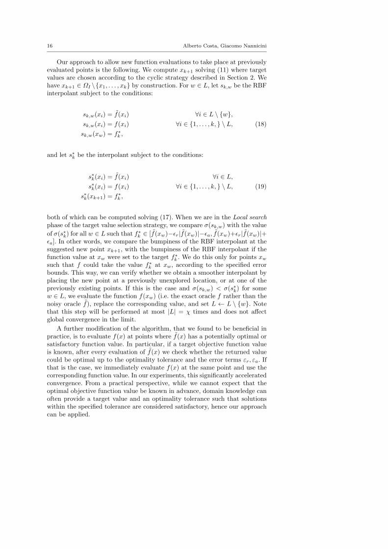
the values f(x1), . . . , f(xχ) by an amount within the allowed error estimatesεr, εa. In particular, instead of solving (4) to determine the interpolant, weintroduce a vector of slack variables ξ ∈ Rk and solve the problem:
min (−1)dmin+1λTΦλs.t.: Φλ+ Ph+ ξ = F
PTλ = 0n+1
∀i ∈ L −εr|f(xi)| − εa ≤ ξi ≤ εr|f(xi)|+ εa∀i ∈ 1, . . . , k \ L ξi = 0.
(17)
Here, F is assumed to contain f(xi) instead of f(xi) for all i ∈ L. Problem (17)minimizes the bumpiness of the RBF interpolant, subject to the interpolationconditions. The inequalities involving ξ allow the interpolant to take any valuewithin the error tolerances εr, εa of the noisy function values f(xi), i ∈ L. Asketch of this idea is given in Figure 2. If we set ξ = 0 for all i, thereby eliminat-ing ξ from the problem, deriving the KKT optimality conditions recovers theoriginal system (4). Note that (17) admits at least one solution if (4) admitsa solution, and (17) is a convex quadratic problem because of the conditionalpositive semidefiniteness of Φ. In practice, to avoid numerical difficulties in thesolution of (17) we use a local solver starting from the solution of (4).
A drawback of this method is that it requires an estimation of ε. A relatedapproach was adopted by [21], whereby all function values are allowed todeviate from the given f(x1), . . . , f(xk), but these deviations are penalizedin the objective function according to a pre-specified penalty parameter. Thedifference between our approach and the one of [21] is that we require tospecify the range within which function values are allowed to vary, whereas[21] requires to specify the value of the penalty parameter in the objectivefunction and computes the error terms accordingly. We believe that estimatinga penalty parameter may prove harder in practice than providing an errorrange, hence our approach may be more natural for practitioners.
16 Alberto Costa, Giacomo Nannicini
Our approach to allow new function evaluations to take place at previouslyevaluated points is the following. We compute xk+1 solving (11) where targetvalues are chosen according to the cyclic strategy described in Section 2. Wehave xk+1 ∈ ΩI \x1, . . . , xk by construction. For w ∈ L, let sk,w be the RBFinterpolant subject to the conditions:
sk,w(xi) = f(xi) ∀i ∈ L \ w,sk,w(xi) = f(xi) ∀i ∈ 1, . . . , k, \ L, (18)
sk,w(xw) = f∗k ,
and let s∗k be the interpolant subject to the conditions:
s∗k(xi) = f(xi) ∀i ∈ L,s∗k(xi) = f(xi) ∀i ∈ 1, . . . , k, \ L, (19)
s∗k(xk+1) = f∗k ,
both of which can be computed solving (17). When we are in the Local searchphase of the target value selection strategy, we compare σ(sk,w) with the value
of σ(s∗k) for all w ∈ L such that f∗k ∈ [f(xw)−εr|f(xw)|−εa, f(xw)+εr|f(xw)|+εa]. In other words, we compare the bumpiness of the RBF interpolant at thesuggested new point xk+1, with the bumpiness of the RBF interpolant if thefunction value at xw were set to the target f∗k . We do this only for points xwsuch that f could take the value f∗k at xw, according to the specified errorbounds. This way, we can verify whether we obtain a smoother interpolant byplacing the new point at a previously unexplored location, or at one of thepreviously existing points. If this is the case and σ(sk,w) < σ(s∗k) for somew ∈ L, we evaluate the function f(xw) (i.e. the exact oracle f rather than thenoisy oracle f), replace the corresponding value, and set L ← L \ w. Notethat this step will be performed at most |L| = χ times and does not affectglobal convergence in the limit.
A further modification of the algorithm, that we found to be beneficial inpractice, is to evaluate f(x) at points where f(x) has a potentially optimal orsatisfactory function value. In particular, if a target objective function valueis known, after every evaluation of f(x) we check whether the returned valuecould be optimal up to the optimality tolerance and the error terms εr, εa. Ifthat is the case, we immediately evaluate f(x) at the same point and use thecorresponding function value. In our experiments, this significantly acceleratedconvergence. From a practical perspective, while we cannot expect that theoptimal objective function value be known in advance, domain knowledge canoften provide a target value and an optimality tolerance such that solutionswithin the specified tolerance are considered satisfactory, hence our approachcan be applied.

A library for black-box optimization 17
5 Computational experiments
In this section we discuss computational experiments performed with RBFOpt,our implementation of the RBF method. All experiments were carried out ona server equipped with four Intel Xeon E5-4620 CPUs (2.20 GHz, 8 cores,Hyper Threading and Turbo Boost disabled) and 128GB RAM (32GB foreach processor), running Linux.
5.1 Implementation
We implemented the RBF method in Python and in MATLAB/Octave. Thetests reported in this paper use our Python implementation, therefore we referto the Python version, that relies on Pyomo [17,16] and the Coopr library. Weuse PyDOE to generate experimental designs, and NumPy for linear algebra.The Python implementation is Python3-compliant, but some of the requiredpackages – most notably Coopr – rely on Python2.7, hence we only supportPython2.7 until all required packages switch to Python3.
Our implementation can be downloaded from the website of the authors.It is open-source and is free for non-commercial academic use: more specifi-cally, academic users are free to use, modify and redistribute the source codeunder the same licensing terms. The exact licensing terms are available on thewebsite.
To solve the nonlinear (mixed-integer in the presence of integer variables)optimization problems generated during the various steps of the algorithm, anonlinear solver is necessary. In our tests, we use IPOPT [34] for continuousproblems, and BONMIN [4] with the NLP-based Branch-and-Bound algorithmfor mixed-integer problems. To optimize nonconvex functions such as (10),we rely on a simple multi-start strategy for IPOPT if there are no integervariables, and on BONMIN’s Branch-and-Bound algorithm in the presence ofinteger variables.
Besides our own version, we are aware of only one available implementa-tion of the RBF method: rbfSolve in the commercial TOMLAB toolkit forMATLAB.
5.2 Test instances
We test our implementation on 26 unconstrained problems taken from the lit-erature, listed in Table 2. We provide more information on the instances below.These problems were originally proposed as a testbed for global optimizationsolvers, and are now considered fairly easy in terms of global optimization.However, they can prove very challenging for black-box solvers that do notexploit analytical information on the problems.
– Dixon-Szego [11] problems: we included the most common instances in thetest set. These instances are the de-facto standard test set used in all com-

18 Alberto Costa, Giacomo Nannicini
Table 2 Details of the instances used for the tests.
Instance Dimension Domain Type Source
branin 2 [−5, 10]× [0, 15] NLP Dixon-Szego [11]camel 2 [−3, 3]× [−2, 2] NLP Dixon-Szego [11]ex4 1 1 1 [−2, 11] NLP GLOBALLIBex4 1 2 1 [1, 2] NLP GLOBALLIBex8 1 1 2 [−1, 2]× [−1, 1] NLP GLOBALLIBex8 1 4 2 [−2, 4]× [−5, 2] NLP GLOBALLIBgear 4 [12, 60]4 MINLP MINLPLib [5]goldsteinprice 2 [−2, 2]2 NLP Dixon-Szego [11]hartman3 3 [0, 1]3 NLP Dixon-Szego [11]hartman6 6 [0, 1]6 NLP Dixon-Szego [11]least 3 [0, 600]× [−200, 200]× [−5, 5] NLP GLOBALLIBnvs04 2 [0, 50]2 MINLP MINLPLib [5]nvs06 2 [1, 50]2 MINLP MINLPLib [5]nvs09 10 [3, 9]10 MINLP MINLPLib [5]nvs16 2 [0, 50]2 MINLP MINLPLib [5]perm0 8 8 [−1, 1]8 NLP Neumaier [25]perm 6 6 [−6, 6]6 NLP Neumaier [25]rbrock 2 [−10, 5]× [−10, 10] NLP GLOBALLIBschoen 10 1 10 [0, 1]10 NLP Schoen [32]schoen 10 2 10 [0, 1]10 NLP Schoen [32]schoen 6 1 6 [0, 1]6 NLP Schoen [32]schoen 6 2 6 [0, 1]6 NLP Schoen [32]shekel10 4 [0, 10]4 NLP Dixon-Szego [11]shekel5 4 [0, 10]4 NLP Dixon-Szego [11]shekel7 4 [0, 10]4 NLP Dixon-Szego [11]
putational evaluations of the RBF method and in many other derivative-free approaches, see e.g. [15,27,19].
– MINLPLib [5] problems: we included all unconstrained instances in thelibrary. For some problems, none of the tested algorithms was able to findthe optimal solution if applied on the problem with the original variablebounds. Therefore, in some cases we restricted the bounds to decrease thedifficulty.
– GLOBALLIB problems: we selected a subset of the unconstrained instancesin the library. Some problems were excluded because too easy or too similarto other problems in our collection.
– Schoen [32] problems: we randomly generated two problems of dimension6 and two of dimension 10. All problems have 50 stationary point, three ofwhich are global minima with value −1000, and the remaining ones attaina value picked uniformly at random in the interval [0, 1000]. Having steepglobal minima allows us to test the performance of our implementationin a situation that is considered difficult to handle for the RBF method,see [27]. Another advantage of using problems of this class is that we canchoose the dimension of the space. In particular, we test problems with 10decision variables, which is larger than most of the instances encounteredin RBF literature. To avoid overrepresentation of a class of instances inour test set, we generate only four random problems of this class.

A library for black-box optimization 19
– Neumaier [25] problems: we included one problem of class “perm”, and oneof class “perm0”, generated with parameters n = 6, β = 60 and n = 8, β =100 respectively. These problems were conceived to be challenging for globaloptimization solvers, and are in our experience very difficult to solve with ablack-box approach. The global minimum of these instances is originally 0,but achieving an optimality tolerance of 1% or 0.01 is essentially hopelessfor these problems. Hence, we translated the functions up by 1000.
An extensive computational evaluation of black-box solvers is discussed in[31], which uses a much larger test set than ours. However, the setting of thatpaper is different because the variable bounds are relatively large, the problemdimension is typically higher, and a larger budget of function evaluations isallowed (up to 2500, while we limit ourselves to 150). The type of problems onwhich the RBF method is expected to perform better is different, and for thesereasons, [31] does not provide computational results for any implementationof the RBF method despite discussing it.
5.3 Comparison of algorithmic settings
The following list summarizes the different settings that we considered, seeSections 2.3 and 3 for details:
– scaling [affine, log, off]: the type of scaling used;– R: restart the algorithm after 6 cycles without improvement of the best
solution found;– B: restricted global minimization of the bumpiness function;– L: if the local search step improves the best solution, it is repeated a second
time;– auto: automatic model selection using cross validation to choose the basis
function
The “default” configuration employs the cubic basis function, a random LatinHypercube design (generated with the maximum minimum distance criterion)for the selection of the first sampling points, no InfStep, and 5 global searchsteps (i.e., κ = 5). This is in accordance with [15,27]. The number of functionevaluations is capped at 150, the time limit for the NLP solver is set to 60seconds, and for the MINLP solver to 120 seconds. We parameterize BONMINto repeat NLP solutions up to 20 times at the root (effectively, this acts asa multi-start approach on nonconvex continuous problems), and 10 times atnodes in case of infeasibility. The time limit for each run is set to 4 hours.Typically, hitting this time limit is indicative of numerical problems in the so-lution process, e.g. the system (4) becomes badly conditioned. If this happens,we consider the corresponding run as a failure.
We evaluate the performance obtained with our implementation on the testinstances of Table 2. Detailed results are given in the Appendix; here we give asummary reporting: the geometric mean of the number of function evaluations
20 Alberto Costa, Giacomo Nannicini
to find a solution within 1% of the global optimum (over 20 runs with differ-ent random seeds – a value of 150 evaluations was used for failed runs), thegeometric standard deviation in parentheses, the total number or successfulruns. Each row represents a different configuration of the algorithm. The bestvalues are in boldface. The geometric means are computed as follows: first,for each instance we compute the arithmetic average of the number of func-tion evaluations. Then, we compute the geometric mean of these arithmeticaverages across the instances. The reason for choosing this approach is thatwithin the same instance, we perform several random trials to get an estimateof the expected number of function evaluations through sampling, hence thearithmetic average is the natural estimator. After obtaining these numbers,we aggregate them with a geometric mean so that each instance is given equalweight, rather than putting more emphasis on problems that require morefunction evaluations (such as problems where the algorithm does not convergewithin the 150 function evaluations).
To compare different versions of the algorithm, we perform a Friedmantest using the average number of function evaluations on each instance asblocks (rows), and the versions of the algorithm as groups (columns). Thenull hypothesis of the test is that there is no difference among the groups.This allows us to assess if one of the algorithms is consistently better thanthe others on the majority of the instances. For details on and assumptionsof the Friedman test, we refer to [8]. Note that the Friedman test does nottake into account the magnitude of the differences among the values, butresults with the Quade test (a non-parametric statistical test that takes intoaccount differences in magnitude) are essentially in agreement, hence we onlyreport results for the Friedman test. All comparisons are performed at the95% significance level. If an algorithm on the row is better (i.e. fewer functionevaluations according to the Friedman test) than an algorithm on the column,we indicate it with a “*”. This is detected using post-hoc analysis when thep-value < 0.05. The p-value is reported in the caption, along with a referenceto the table(s) in the Appendix with the detailed results.
We would like to answer the following research questions:
1. Which algorithmic configuration is the best, and in particular, are theimprovements of Section 2.3 beneficial in practice?
2. Is our approach to handle noisy function evaluations effective?3. Is automatic model selection using cross validation beneficial in practice?4. Is our implementation competitive with the state-of-the-art?5. Can the surrogate models produced by the algorithm be useful to perform
sensitivity analysis around the optimum?
The first question is investigated in the rest of this section. The second andthe third questions are investigated in Sections 5.4-5.5. The fourth question isdiscussed in Section 5.6. The fifth question is discussed in Section 5.7.
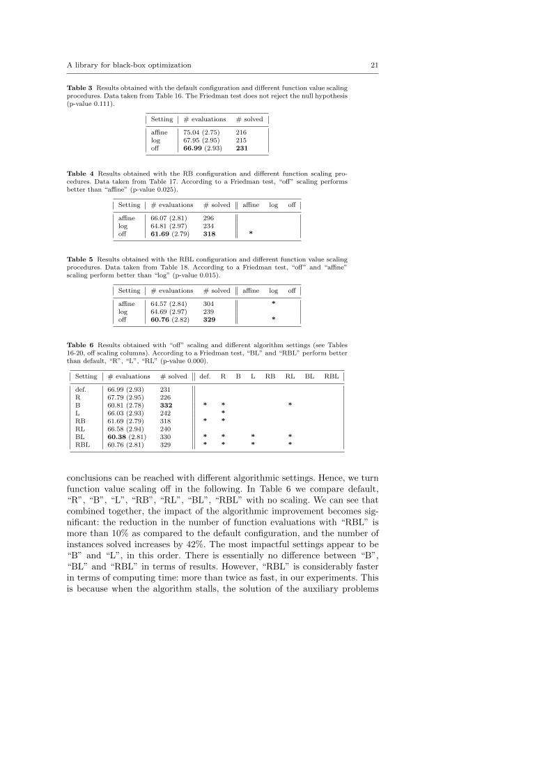
We report the performance of with different settings of the algorithms anddifferent scaling procedures in Tables 3-5. It appears that “off” scaling is al-ways not worse and sometimes better than other scaling procedures. Similar
A library for black-box optimization 21
Table 3 Results obtained with the default configuration and different function value scalingprocedures. Data taken from Table 16. The Friedman test does not reject the null hypothesis(p-value 0.111).
Setting # evaluations # solved
affine 75.04 (2.75) 216log 67.95 (2.95) 215off 66.99 (2.93) 231
Table 4 Results obtained with the RB configuration and different function scaling pro-cedures. Data taken from Table 17. According to a Friedman test, “off” scaling performsbetter than “affine” (p-value 0.025).
Setting # evaluations # solved affine log off
affine 66.07 (2.81) 296log 64.81 (2.97) 234off 61.69 (2.79) 318 *
Table 5 Results obtained with the RBL configuration and different function value scalingprocedures. Data taken from Table 18. According to a Friedman test, “off” and “affine”scaling perform better than “log” (p-value 0.015).
Setting # evaluations # solved affine log off
affine 64.57 (2.84) 304 *log 64.69 (2.97) 239off 60.76 (2.82) 329 *
Table 6 Results obtained with “off” scaling and different algorithm settings (see Tables16-20, off scaling columns). According to a Friedman test, “BL” and “RBL” perform betterthan default, “R”, “L”, “RL” (p-value 0.000).
Setting # evaluations # solved def. R B L RB RL BL RBL
def. 66.99 (2.93) 231R 67.79 (2.95) 226B 60.81 (2.78) 332 * * *L 66.03 (2.93) 242 *RB 61.69 (2.79) 318 * *RL 66.58 (2.94) 240BL 60.38 (2.81) 330 * * * *RBL 60.76 (2.81) 329 * * * *
conclusions can be reached with different algorithmic settings. Hence, we turnfunction value scaling off in the following. In Table 6 we compare default,“R”, “B”, “L”, “RB”, “RL”, “BL”, “RBL” with no scaling. We can see thatcombined together, the impact of the algorithmic improvement becomes sig-nificant: the reduction in the number of function evaluations with “RBL” ismore than 10% as compared to the default configuration, and the number ofinstances solved increases by 42%. The most impactful settings appear to be“B” and “L”, in this order. There is essentially no difference between “B”,“BL” and “RBL” in terms of results. However, “RBL” is considerably fasterin terms of computing time: more than twice as fast, in our experiments. Thisis because when the algorithm stalls, the solution of the auxiliary problems
22 Alberto Costa, Giacomo Nannicini
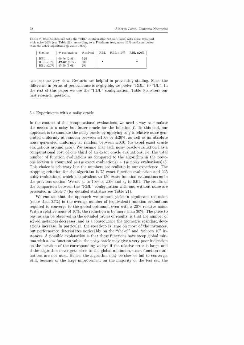
Table 7 Results obtained with the “RBL” configuration without noise, with noise 10%, andwith noise 20% (see Table 21). According to a Friedman test, noise 10% performs betterthan the other algorithms (p-value 0.006).
Setting # evaluations # solved RBL RBL n10% RBL n20%
RBL 60.76 (2.81) 329RBL n10% 42.67 (3.77) 300 * *RBL n20% 45.50 (3.61) 293
can become very slow. Restarts are helpful in preventing stalling. Since thedifference in terms of performance is negligible, we prefer “RBL” to “BL”. Inthe rest of this paper we use the “RBL” configuration. Table 6 answers ourfirst research question.
5.4 Experiments with a noisy oracle
In the context of this computational evaluations, we need a way to simulatethe access to a noisy but faster oracle for the function f . To this end, ourapproach is to simulate the noisy oracle by applying to f a relative noise gen-erated uniformly at random between ±10% or ±20%, as well as an absolutenoise generated uniformly at random between ±0.01 (to avoid exact oracleevaluations around zero). We assume that each noisy oracle evaluation has acomputational cost of one third of an exact oracle evaluations, i.e. the totalnumber of function evaluations as compared to the algorithm in the previ-ous section is computed as (# exact evaluations) + (# noisy evaluations)/3.This choice is arbitrary but the numbers are realistic in our experience. Thestopping criterion for the algorithm is 75 exact function evaluation and 225noisy evaluations, which is equivalent to 150 exact function evaluations as inthe previous section. We set εr to 10% or 20% and εa to 0.01. The results ofthe comparison between the “RBL” configuration with and without noise arepresented in Table 7 (for detailed statistics see Table 21).
We can see that the approach we propose yields a significant reduction(more than 25%) in the average number of (equivalent) function evaluationsrequired to converge to the global optimum, even with a 20% relative noise.With a relative noise of 10%, the reduction is by more than 30%. The price topay, as can be observed in the detailed tables of results, is that the number ofsolved instances decreases, and as a consequence the geometric standard devi-ations increase. In particular, the speed-up is large on most of the instances,but performance deteriorates noticeably on the “shekel” and “schoen 10” in-stances. A possible explanation is that these functions have steep global min-ima with a low function value: the noisy oracle may give a very poor indicationon the location of the corresponding valleys if the relative error is large, andif the algorithm never gets close to the global minimum, exact function eval-uations are not used. Hence, the algorithm may be slow or fail to converge.Still, because of the large improvement on the majority of the test set, the
A library for black-box optimization 23
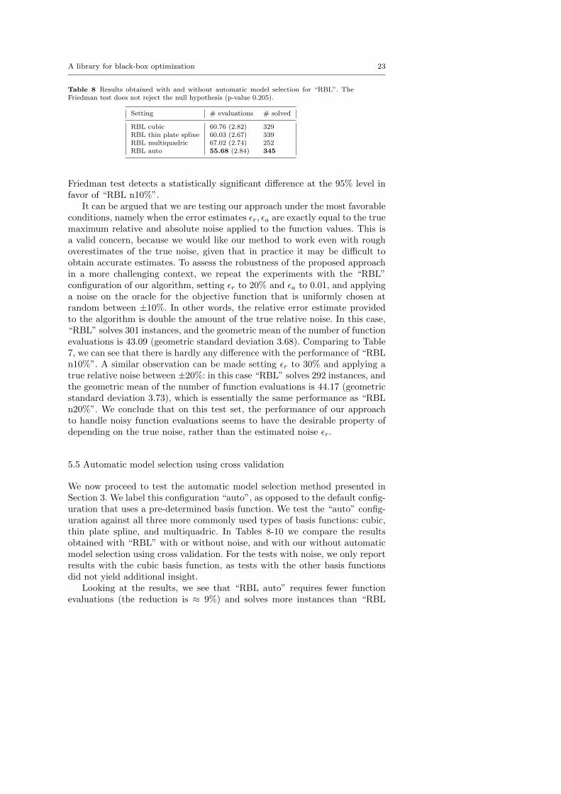
Table 8 Results obtained with and without automatic model selection for “RBL”. TheFriedman test does not reject the null hypothesis (p-value 0.205).
Setting # evaluations # solved
RBL cubic 60.76 (2.82) 329RBL thin plate spline 60.03 (2.67) 339RBL multiquadric 67.02 (2.74) 252RBL auto 55.68 (2.84) 345
Friedman test detects a statistically significant difference at the 95% level infavor of “RBL n10%”.
It can be argued that we are testing our approach under the most favorableconditions, namely when the error estimates εr, εa are exactly equal to the truemaximum relative and absolute noise applied to the function values. This isa valid concern, because we would like our method to work even with roughoverestimates of the true noise, given that in practice it may be difficult toobtain accurate estimates. To assess the robustness of the proposed approachin a more challenging context, we repeat the experiments with the “RBL”configuration of our algorithm, setting εr to 20% and εa to 0.01, and applyinga noise on the oracle for the objective function that is uniformly chosen atrandom between ±10%. In other words, the relative error estimate providedto the algorithm is double the amount of the true relative noise. In this case,“RBL” solves 301 instances, and the geometric mean of the number of functionevaluations is 43.09 (geometric standard deviation 3.68). Comparing to Table7, we can see that there is hardly any difference with the performance of “RBLn10%”. A similar observation can be made setting εr to 30% and applying atrue relative noise between ±20%: in this case “RBL” solves 292 instances, andthe geometric mean of the number of function evaluations is 44.17 (geometricstandard deviation 3.73), which is essentially the same performance as “RBLn20%”. We conclude that on this test set, the performance of our approachto handle noisy function evaluations seems to have the desirable property ofdepending on the true noise, rather than the estimated noise εr.
5.5 Automatic model selection using cross validation
We now proceed to test the automatic model selection method presented inSection 3. We label this configuration “auto”, as opposed to the default config-uration that uses a pre-determined basis function. We test the “auto” config-uration against all three more commonly used types of basis functions: cubic,thin plate spline, and multiquadric. In Tables 8-10 we compare the resultsobtained with “RBL” with or without noise, and with our without automaticmodel selection using cross validation. For the tests with noise, we only reportresults with the cubic basis function, as tests with the other basis functionsdid not yield additional insight.
Looking at the results, we see that “RBL auto” requires fewer functionevaluations (the reduction is ≈ 9%) and solves more instances than “RBL

24 Alberto Costa, Giacomo Nannicini
Table 9 Results obtained with and without automatic model selection for “RBL” with noiselevel 10% (see Table 23). The Friedman test does not reject the null hypothesis (p-value0.503).
Setting # evaluations # solved
RBL n10% cubic 42.68 (3.77) 300RBL n10% auto 40.87 (3.59) 320
Table 10 Results obtained with and without automatic model selection for “RBL” withnoise level 20%. The Friedman test does not reject the null hypothesis (p-value 0.832)
Setting # evaluations # solved
RBL n20% cubic 45.50 (3.60) 293RBL n20% auto 45.38 (3.57) 303
cubic” or “RBL thin plate spline”, although the difference is not detected bya Friedman test. This is our best performing algorithm configuration so far,solving more instances than any other tested configuration and showing thatthe automatic model selection is useful in our experiments. In particular, auto-matic model selection improves over any one of the three tested basis function,suggesting that it is able to find the best performing model. It is interesting tocompare our “auto” configuration with the best single basis function for eachinstance, i.e. the results that could be obtained in the hypothetical situationof being able to guess the best performing basis function before solving theinstance. This “RBL best-basis-function” would require on average 54.33 func-tion evaluations (geometric standard deviation 2.81), solving 364 instances,and is therefore only marginally better than “RBL auto” on our test set. Theresults suggest that our model selection scheme is able to correctly guess thebest surrogate model in most situations.
The same results carry over when exploiting a noisy oracle with relativeerror at most 10%: automatic model selection is able to reduce the numberof function evaluations by ≈ 7%, and solves more instances. However, with arelative noise of 20%, the benefit from using automatic model selection thinsout considerably and is hardly noticeable. This can be explained with the factthat automatic model selection relies on the function evaluations to assessmodel performance: in a context where the function evaluations are affectedby a significant relative error, assessing model quality becomes difficult, andtherefore our proposed procedure brings little advantage. Still, even with alarge noise our “auto” configuration is no worse than the default one and findsthe global optimum on a few more instances. This answers our third researchquestion.
5.6 Comparison with the literature
In this section we investigate how our implementation compares with resultsfrom the literature. The testbed for this section consists of the seven Dixon-
A library for black-box optimization 25
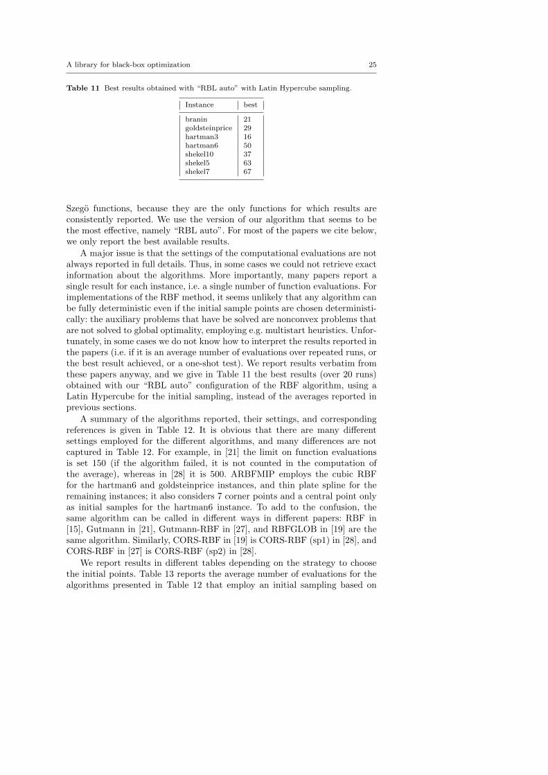
Table 11 Best results obtained with “RBL auto” with Latin Hypercube sampling.
Instance best
branin 21goldsteinprice 29hartman3 16hartman6 50shekel10 37shekel5 63shekel7 67
Szego functions, because they are the only functions for which results areconsistently reported. We use the version of our algorithm that seems to bethe most effective, namely “RBL auto”. For most of the papers we cite below,we only report the best available results.
A major issue is that the settings of the computational evaluations are notalways reported in full details. Thus, in some cases we could not retrieve exactinformation about the algorithms. More importantly, many papers report asingle result for each instance, i.e. a single number of function evaluations. Forimplementations of the RBF method, it seems unlikely that any algorithm canbe fully deterministic even if the initial sample points are chosen deterministi-cally: the auxiliary problems that have be solved are nonconvex problems thatare not solved to global optimality, employing e.g. multistart heuristics. Unfor-tunately, in some cases we do not know how to interpret the results reported inthe papers (i.e. if it is an average number of evaluations over repeated runs, orthe best result achieved, or a one-shot test). We report results verbatim fromthese papers anyway, and we give in Table 11 the best results (over 20 runs)obtained with our “RBL auto” configuration of the RBF algorithm, using aLatin Hypercube for the initial sampling, instead of the averages reported inprevious sections.
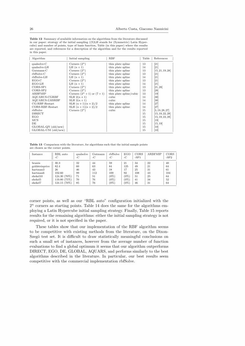
A summary of the algorithms reported, their settings, and correspondingreferences is given in Table 12. It is obvious that there are many differentsettings employed for the different algorithms, and many differences are notcaptured in Table 12. For example, in [21] the limit on function evaluationsis set 150 (if the algorithm failed, it is not counted in the computation ofthe average), whereas in [28] it is 500. ARBFMIP employs the cubic RBFfor the hartman6 and goldsteinprice instances, and thin plate spline for theremaining instances; it also considers 7 corner points and a central point onlyas initial samples for the hartman6 instance. To add to the confusion, thesame algorithm can be called in different ways in different papers: RBF in[15], Gutmann in [21], Gutmann-RBF in [27], and RBFGLOB in [19] are thesame algorithm. Similarly, CORS-RBF in [19] is CORS-RBF (sp1) in [28], andCORS-RBF in [27] is CORS-RBF (sp2) in [28].
We report results in different tables depending on the strategy to choosethe initial points. Table 13 reports the average number of evaluations for thealgorithms presented in Table 12 that employ an initial sampling based on
26 Alberto Costa, Giacomo Nannicini
Table 12 Summary of available information on the algorithms from the literature discussedin our paper: strategy of the initial sampling ((S)LH stands for (Symmetric) Latin Hyper-cube) and number of points, type of basis function, Table (in this paper) where the resultsare reported, and references for a description of the algorithm and for the results reportedin this paper.
Algorithm Initial sampling RBF Table References
qualsolve-C Corners (2n) thin plate spline 13 [21]qualsolve-LH LH (n+ 1) thin plate spline 14 [21]Gutmann-C Corners (2n) thin plate spline 13 [15,21,19,28]rbfSolve-C Corners (2n) thin plate spline 13 [21]rbfSolve-LH LH (n+ 1) thin plate spline 14 [21]EGO-C Corners (2n) thin plate spline 13 [21]EGO-LH LH (n+ 1) thin plate spline 14 [21]CORS-SP1 Corners (2n) thin plate spline 13 [21,28]CORS-SP2 Corners (2n) thin plate spline 13 [28]ARBFMIP Corners (2n + 1) or (7 + 1) thin plate spline/cubic 13 [19]AQUARUS-CGRBF SLH 2(n+ 1) cubic 14 [30]AQUARUS-LMSRBF SLH 2(n+ 1) cubic 14 [30]CG-RBF-Restart SLH (n+ 1)(n+ 2)/2 thin plate spline 14 [27]CORS-RBF-Restart SLH (n+ 1)(n+ 2)/2 thin plate spline 14 [27]rbfSolve Corners (2n) cubic 15 [3,19,28,27]DIRECT 15 [15,19,22,28]EGO 15 [15,19,23,28]MCS 15 [19]DE 15 [15,19]GLOBAL-QN (old/new) 15 [10]GLOBAL-UNI (old/new) 15 [10]
Table 13 Comparison with the literature, for algorithms such that the initial sample pointsare chosen as the corner points.
Instance RBL auto qualsolve Gutmann rbfSolve EGO CORS ARBFMIP CORS-C -C -C -C -C -SP1 -SP2
branin 30.3 32 44 59 21 34 22 40goldsteinprice 82.4 60 63 84 125 49 21 64hartman3 26 46 43 18 17 25 31 61hartman6 102.60 99 112 109 92 108 43 104shekel10 124.30 (70%) 71 51 (0%) (0%) 51 25 64shekel5 119.80 (75%) 70 76 (0%) (0%) 41 34 52shekel7 124.15 (70%) 85 76 (0%) (0%) 46 31 64
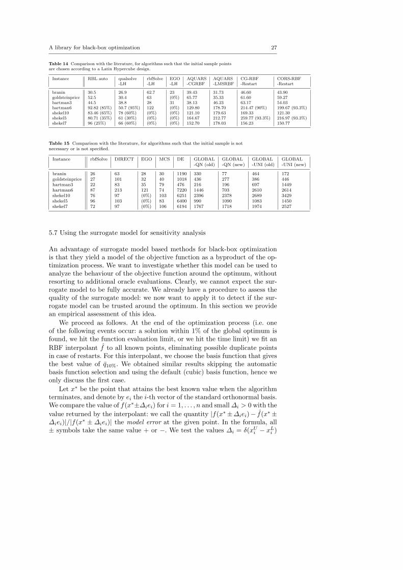
corner points, as well as our “RBL auto” configuration initialized with the2n corners as starting points. Table 14 does the same for the algorithms em-ploying a Latin Hypercube initial sampling strategy. Finally, Table 15 reportsresults for the remaining algorithms: either the initial sampling strategy is notrequired, or it is not specified in the paper.
These tables show that our implementation of the RBF algorithm seemsto be competitive with existing methods from the literature, on the Dixon-Szego test set. It is difficult to draw statistically meaningful conclusions onsuch a small set of instances, however from the average number of functionevaluations to find a global optimum it seems that our algorithm outperformsDIRECT, EGO, DE, GLOBAL, AQUARS, and performs similarly to the bestalgorithms described in the literature. In particular, our best results seemcompetitive with the commercial implementation rbfSolve.
A library for black-box optimization 27
Table 14 Comparison with the literature, for algorithms such that the initial sample pointsare chosen according to a Latin Hypercube design.
Instance RBL auto qualsolve rbfSolve EGO AQUARS AQUARS CG-RBF CORS-RBF-LH -LH -LH -CGRBF -LMSRBF -Restart -Restart
branin 30.5 26.9 62.7 23 39.43 31.73 46.60 43.90goldsteinprice 52.5 30.4 63 (0%) 65.77 35.33 61.60 59.27hartman3 44.5 38.8 28 31 38.13 46.23 63.17 54.03hartman6 92.82 (85%) 50.7 (95%) 122 (0%) 129.80 178.70 214.47 (90%) 199.67 (93.3%)shekel10 83.46 (65%) 78 (60%) (0%) (0%) 121.10 179.63 169.33 121.30shekel5 80.71 (35%) 61 (30%) (0%) (0%) 164.67 212.77 259.77 (93.3%) 216.97 (93.3%)shekel7 96 (25%) 66 (60%) (0%) (0%) 152.70 178.03 156.23 150.77
Table 15 Comparison with the literature, for algorithms such that the initial sample is notnecessary or is not specified.
Instance rbfSolve DIRECT EGO MCS DE GLOBAL GLOBAL GLOBAL GLOBAL-QN (old) -QN (new) -UNI (old) -UNI (new)
branin 26 63 28 30 1190 330 77 464 172goldsteinprice 27 101 32 40 1018 436 277 386 446hartman3 22 83 35 79 476 216 196 697 1449hartman6 87 213 121 74 7220 1446 703 2610 2614shekel10 76 97 (0%) 103 6251 2396 2378 2689 3429shekel5 96 103 (0%) 83 6400 990 1090 1083 1450shekel7 72 97 (0%) 106 6194 1767 1718 1974 2527
5.7 Using the surrogate model for sensitivity analysis
An advantage of surrogate model based methods for black-box optimizationis that they yield a model of the objective function as a byproduct of the op-timization process. We want to investigate whether this model can be used toanalyze the behaviour of the objective function around the optimum, withoutresorting to additional oracle evaluations. Clearly, we cannot expect the sur-rogate model to be fully accurate. We already have a procedure to assess thequality of the surrogate model: we now want to apply it to detect if the sur-rogate model can be trusted around the optimum. In this section we providean empirical assessment of this idea.
We proceed as follows. At the end of the optimization process (i.e. oneof the following events occur: a solution within 1% of the global optimum isfound, we hit the function evaluation limit, or we hit the time limit) we fit an
RBF interpolant f to all known points, eliminating possible duplicate pointsin case of restarts. For this interpolant, we choose the basis function that givesthe best value of q10%. We obtained similar results skipping the automaticbasis function selection and using the default (cubic) basis function, hence weonly discuss the first case.
Let x∗ be the point that attains the best known value when the algorithmterminates, and denote by ei the i-th vector of the standard orthonormal basis.We compare the value of f(x∗±∆iei) for i = 1, . . . , n and small∆i > 0 with the
value returned by the interpolant: we call the quantity |f(x∗±∆iei)− f(x∗±∆iei)|/|f(x∗ ± ∆iei)| the model error at the given point. In the formula, all± symbols take the same value + or −. We test the values ∆i = δ(xUi − xLi )

28 Alberto Costa, Giacomo Nannicini
0
20
40
60
80
100
0 5 10 15 Infty
Perc
enta
ge
Threshold
accurate at stepsize 0.005accurate at stepsize 0.01accurate at stepsize 0.02accurate at stepsize 0.05accurate at stepsize 0.1
model trusted0
20
40
60
80
100
0 5 10 15 Infty
Perc
enta
ge
Threshold
accurate at stepsize 0.005accurate at stepsize 0.01accurate at stepsize 0.02accurate at stepsize 0.05accurate at stepsize 0.1
model trusted
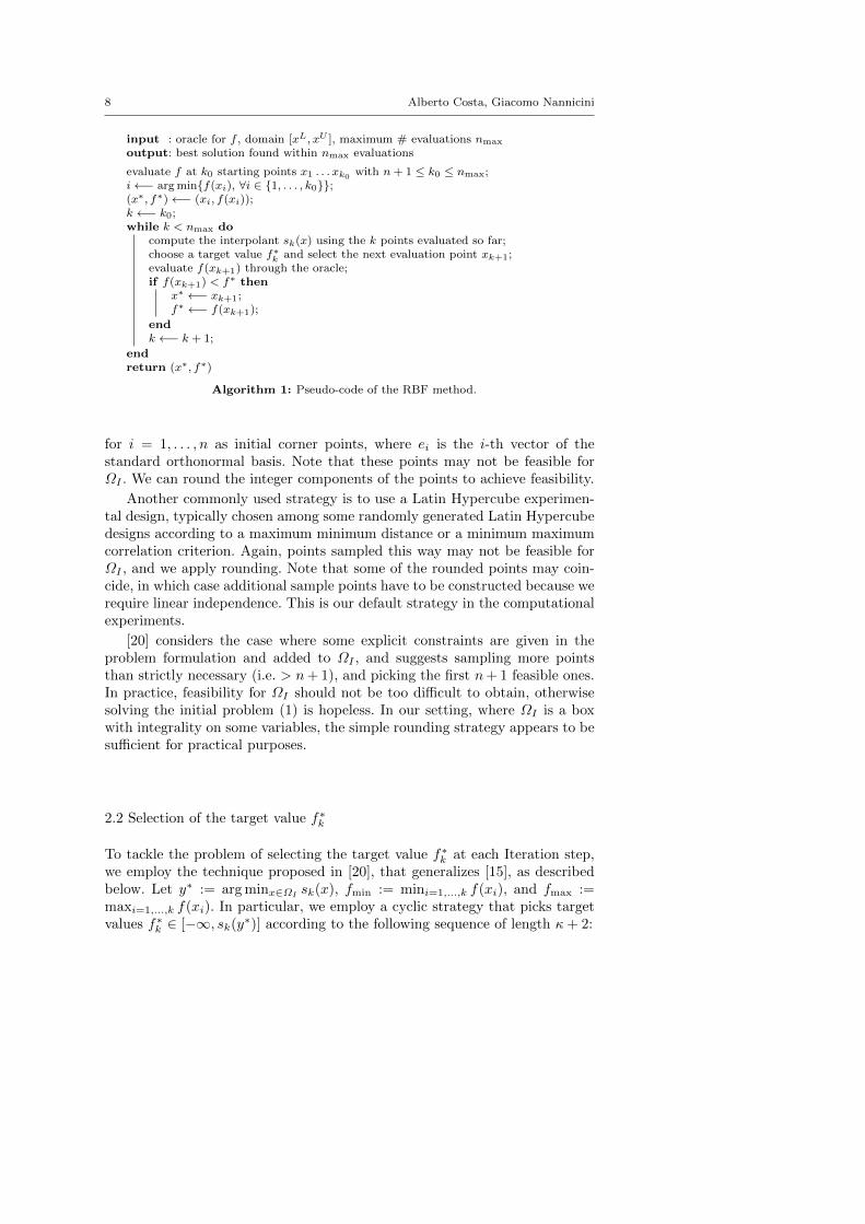
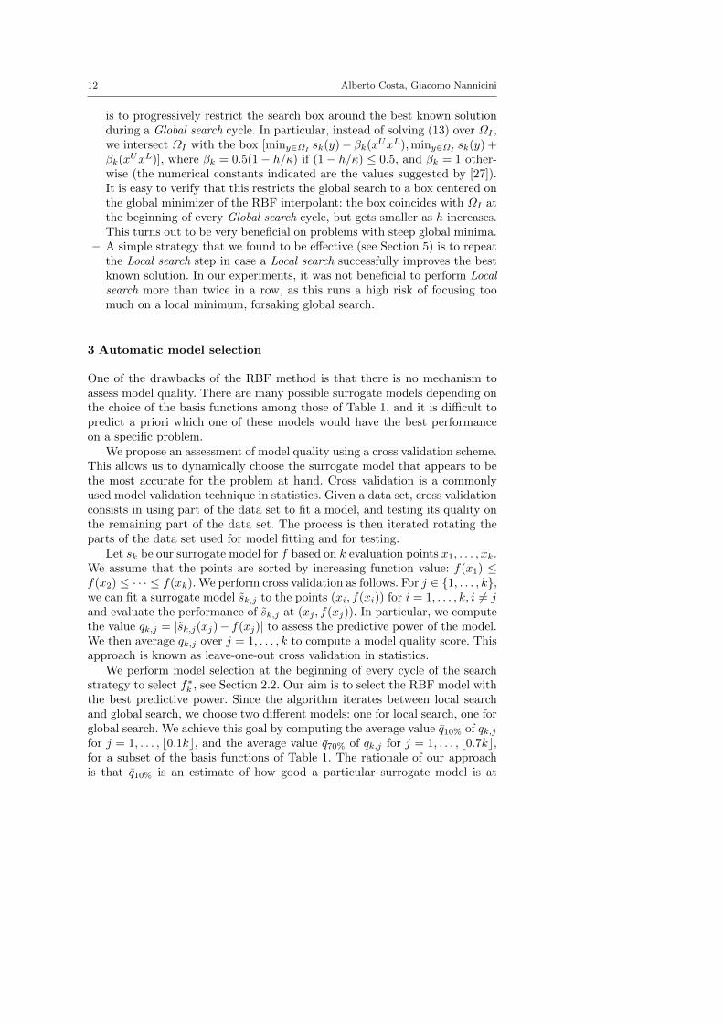
Fig. 3 Percentage of surrogate models that are trusted and corresponding percentage ofmodel errors that are below 10%, for threshold policies of the form q10% ≤ x (left figure)and q20% ≤ x (right figure), where x is the value on the x-axis. The left axis goes from 0to 20 with 0.5 increments, but the last point is out-of-scale and indicates x = ∞ (label:“Infty”).
for δ = 0.005, 0.01, 0.02, 0.05, 0.1. Our main question is whether the values qk%provide useful information about the accuracy of the model for some values ofk. We plotted graphs of qk% for k = 10, 20, . . . , 100 against the model errors.This is a large amount of data; we report a summary of our findings.
For practical purposes, we decided that model errors of more than 10% arenot acceptable, and that we are looking for a simple threshold policy for qk%to determine whether or not the surrogate model should be trusted aroundthe optimum. For the tested values of k%, we tried different thresholds t andplotted the aggregated model errors. We plot these graphs for k = 10, 20 inFigure 3, where we give the fraction of model errors (among all points withinthe domain located ±∆iei away from x∗, i = 1, . . . , n) that are below 10%,and the fractions of models that are trusted based on the given threshold.Ideally, we want these values to be as high as possible; for k ≥ 30, all thecurves are shifted noticeably towards the bottom, therefore we do not reportthe corresponding results. From the graphs, it seems that q20% ≤ 10% performsrelatively well in practice: up to δ = 0.02, about 75% of the time the modelerrors stay below 10%.
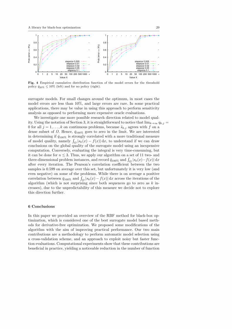
A natural question is to determine if there is benefit in using the thresholdpolicy for q20% as compared to simply trusting the model every time. To answerthis question, in Figure 4 we compare the model errors for the models thatare trusted by our threshold policy, to the errors for all the models. We cansee that the reduction is significant. Using our policy, ≈ 60% of the errors arewithin 1% for δ = 0.01, and more importantly, in almost 90% of the cases theerrors are smaller than 50%, whereas without the threshold policy we observea significant fraction of the errors above 50%.
To summarize, one should not expect that the surrogate model can alwayspredict the unknown objective function with high accuracy. However, in ourexperiments evaluating the quality of the model via cross-validation is helpfulin assessing model accuracy: using a simple threshold policy on a measureof model quality, we are able to identify a large number of the inaccurate
A library for black-box optimization 29
0
0.2
0.4
0.6
0.8
1
0 1 2 5 10 20 50 100 200 500 1000 +
Pro
b (
err
or
<=
X%
)
Value X
stepsize 0.005stepsize 0.01stepsize 0.02stepsize 0.05stepsize 0.1
0
0.2
0.4
0.6
0.8
1
0 1 2 5 10 20 50 100 200 500 1000 +
Pro
b (
err
or
<=
X%
)
Value X
stepsize 0.005stepsize 0.01stepsize 0.02stepsize 0.05stepsize 0.1
Fig. 4 Empirical cumulative distribution function of the model errors for the thresholdpolicy q20% ≤ 10% (left) and for no policy (right).
surrogate models. For small changes around the optimum, in most cases themodel errors are less than 10%, and large errors are rare. In some practicalapplications, there may be value in using this approach to perform sensitivityanalysis as opposed to performing more expensive oracle evaluations.
We investigate one more possible research direction related to model qual-ity. Using the notation of Section 3, it is straightforward to notice that limk→∞ qk,j =0 for all j = 1, . . . , k on continuous problems, because sk,j agrees with f on adense subset of Ω. Hence, q100% goes to zero in the limit. We are interestedin determining if q100% is strongly correlated with a more traditional measureof model quality, namely
∫Ω|sk(x) − f(x)|dx, to understand if we can draw
conclusions on the global quality of the surrogate model using an inexpensivecomputation. Conversely, evaluating the integral is very time-consuming, butit can be done for n ≤ 3. Thus, we apply our algorithm on a set of 11 two- andthree-dimensional problem instances, and record q100% and
∫Ω|sk(x)−f(x)|dx
after every iteration. The Pearson’s correlation coefficient between the twosamples is 0.599 on average over this set, but unfortunately it is very low (andeven negative) on some of the problems. While there is on average a positivecorrelation between q100% and
∫Ω|sk(x)− f(x)|dx across the iterations of the
algorithm (which is not surprising since both sequences go to zero as k in-creases), due to the unpredictability of this measure we decide not to explorethis direction further.
6 Conclusions
In this paper we provided an overview of the RBF method for black-box op-timization, which is considered one of the best surrogate model based meth-ods for derivative-free optimization. We proposed some modifications of thealgorithm with the aim of improving practical performance. Our two maincontributions are a methodology to perform automatic model selection usinga cross-validation scheme, and an approach to exploit noisy but faster func-tion evaluations. Computational experiments show that these contributions arebeneficial in practice, yielding a noticeable reduction in the number of function

30 Alberto Costa, Giacomo Nannicini
evaluations to achieve convergence to within 1% of the global optimum on acollection of test problems taken from the literature.
Our implementation of the algorithm is open-source and available in alibrary called RBFOpt, which is free for noncommercial academic use. A com-parison with other implementations of the RBF algorithm, as well as othermethods from the literature, shows that RBFOpt is competitive with the bestperforming methods available, including commercial software.
Acknowledgements The authors are grateful for the financial support by the SUTD-MITInternational Design Center under grant IDG21300102.
References
1. Achterberg, T.: SCIP: Solving constraint integer programs. Mathematical ProgrammingComputation 1(1), 1–41 (2009)
2. Baudoui, V.: Optimisation robuste multiobjectifs par modeles de substitution. Ph.D.thesis, University of Toulouse Paul Sabatier (2012)
3. Bjorkman, M., Holmstrom, K.: Global optimization of costly nonconvex functions usingradial basis functions. Optimization and Engineering 1(4), 373–397 (2000)
4. Bonami, P., Biegler, L., Conn, A., Cornuejols, G., Grossmann, I., Laird, C., Lee, J.,Lodi, A., Margot, F., Sawaya, N., Wachter, A.: An algorithmic framework for convexMixed Integer Nonlinear Programs. Discrete Optimization 5, 186–204 (2008)
5. Bussieck, M.R., Drud, A.S., Meeraus, A.: MINLPLib — a collection of test modelsfor Mixed-Integer Nonlinear Programming. INFORMS Journal on Computing 15(1)(2003). URL http://www.gamsworld.org/minlp/minlplib.htm
6. Conn, A.R., Scheinberg, K., Toint, P.L.: Recent progress in unconstrained nonlinearoptimization without derivatives. Mathematical Programming 79(1-3), 397–414 (1997).DOI 10.1007/BF02614326
7. Conn, A.R., Scheinberg, K., Vicente, L.N.: Introduction to Derivative-Free Optimiza-tion. MPS-SIAM Series on Optimization. Society for Industrial and Applied Mathe-matics (2009)
8. Conover, W.J.: Practical Nonparametric Statistics, 3rd edition. Wiley (1999)9. Costa, A., Nannicini, G., Schroepfer, T., Wortmann, T.: Black-box optimization of
lighting simulation in architectural design. In: CSD&M Asia 2014. Springer (2014).Accepted for publication
10. Csendes, T., Pal, L., Sendn, J.O.H., Banga, J.R.: The global optimization method re-visited. Optimization Letters 2(4), 445–454 (2008)
11. Dixon, L., Szego, G.: The global optimization problem: an introduction. In: L. Dixon,G. Szego (eds.) Towards Global Optimization, pp. 1–15. North Holland, Amsterdam(1975)
12. Gendreau, M., Potvin, J.Y. (eds.): Handbook of Metaheuristics, 2nd edition. Kluwer,Dordrecht (2010)
13. Glover, F., Kochenberger, G. (eds.): Handbook of Metaheuristics. Kluwer, Dordrecht(2003)
14. Gomes, C.P., Selman, B., Crato, N., Kautz, H.: Heavy-tailed phenomena in satisfiabilityand constraint satisfaction problems. Journal of Automated Reasoning 24(1-2), 67–100(2000). DOI 10.1023/A:1006314320276
15. Gutmann, H.M.: A radial basis function method for global optimization. Journal ofGlobal Optimization 19, 201–227 (2001). 10.1023/A:1011255519438
16. Hart, W.E., Laird, C., Watson, J.P., Woodruff, D.L.: Pyomo – Optimization Modelingin Python, Springer Optimization and Its Applications, vol. 67. Springer (2012)
17. Hart, W.E., Watson, J.P., Woodruff, D.L.: Pyomo: modeling and solving mathematicalprograms in python. Mathematical Programming Computation 3(3), 219–260 (2011).DOI 10.1007/s12532-011-0026-8

A library for black-box optimization 31
18. Hemker, T.: Derivative free surrogate optimization for mixed-integer nonlinear black-box problems in engineering. Master’s thesis, Technischen Universitat Darmstadt (2008)
19. Holmstrom, K.: An adaptive radial basis algorithm (ARBF) for expensive black-boxglobal optimization. Journal of Global Optimization 41(3), 447–464 (2008)
20. Holmstrom, K., Quttineh, N.H., Edvall, M.M.: An adaptive radial basis algorithm (arbf)for expensive black-box mixed-integer constrained global optimization. Optimizationand Engineering 9(4), 311–339 (2008)
21. Jakobsson, S., Patriksson, M., Rudholm, J., Wojciechowski, A.: A method for simulationbased optimization using radial basis functions. Optimization and Engineering 11(4),501–532 (2010)
22. Jones, D., Perttunen, C., Stuckman, B.: Lipschitzian optimization without the lipschitzconstant. Journal of Optimization Theory and Applications 79(1), 157–181 (1993)
23. Jones, D., Schonlau, M., Welch, W.: Efficient global optimization of expensive black-boxfunctions. Journal of Global optimization 13(4), 455–492 (1998)
24. Kolda, T.G., Lewis, R.M., Torczon, V.J.: Optimization by direct search: new perspec-tives on some classical and modern methods. SIAM Review 45(3), 385–482 (2003)
25. Neumaier, A.: Neumaier’s collection of test problems for global optimization. URL http:
//www.mat.univie.ac.at/~neum/glopt/my_problems.html. Retrieved in May 201426. Powell, M.: Recent research at cambridge on radial basis functions. In: New Develop-
ments in Approximation Theory, International Series of Numerical Mathematics, vol.132, pp. 215–232. Birkhauser Verlag, Basel (1999)
27. Regis, R., Shoemaker, C.: Improved strategies for radial basis function methodsfor global optimization. Journal of Global Optimization 37, 113–135 (2007).10.1007/s10898-006-9040-1
28. Regis, R.G., Shoemaker, C.A.: Constrained global optimization of expensive black boxfunctions using radial basis functions. Journal of Global Optimization 31(1), 153–171(2005)
29. Regis, R.G., Shoemaker, C.A.: A stochastic radial basis function method for the globaloptimization of expensive functions. INFORMS Journal on Computing 19(4), 497–509(2007). DOI 10.1287/ijoc.1060.0182
30. Regis, R.G., Shoemaker, C.A.: A quasi-multistart framework for global optimizationof expensive functions using response surface models. Journal of Global Optimization56(4), 1719–1753 (2013)
31. Rios, L.M., Sahinidis, N.V.: Derivative-free optimization: a review of algorithms andcomparison of software implementations. Journal of Global Optimization 56(3), 1247–1293 (2013)
32. Schoen, F.: A wide class of test functions for global optimization. Journal of GlobalOptimization 3(2), 133–137 (1993)
33. Torn, A., Zilinskas: Global optimization. Springer (1987)34. Wachter, A., Biegler, L.T.: On the implementation of a primal-dual interior point filter
line search algorithm for large-scale nonlinear programming. Mathematical Program-ming 106(1), 25–57 (2006)
Tables of results
The details of the numerical results obtained with the RBF algorithm are presented in Tables16-25. For each instance we perform 20 runs of the algorithm, changing the random seed.The algorithm fails if it cannot find a solution having a relative error less than or equal to1% from the global optimum within 150 function evaluations. The relative error is computedas |f∗ −F ∗|/|F ∗|, where f∗ is the best solution found and F ∗ is the global optimum of theproblem. In case of F ∗ = 0, the error is computed as |f∗ − F ∗|. The statistics presentedon the tables are the number of successful trials out of 20 (“#sol.”), the average number offunction evaluations, the standard deviation from the mean, and the average relative errorafter 150 evaluations for those instances where the algorithm does not converge.
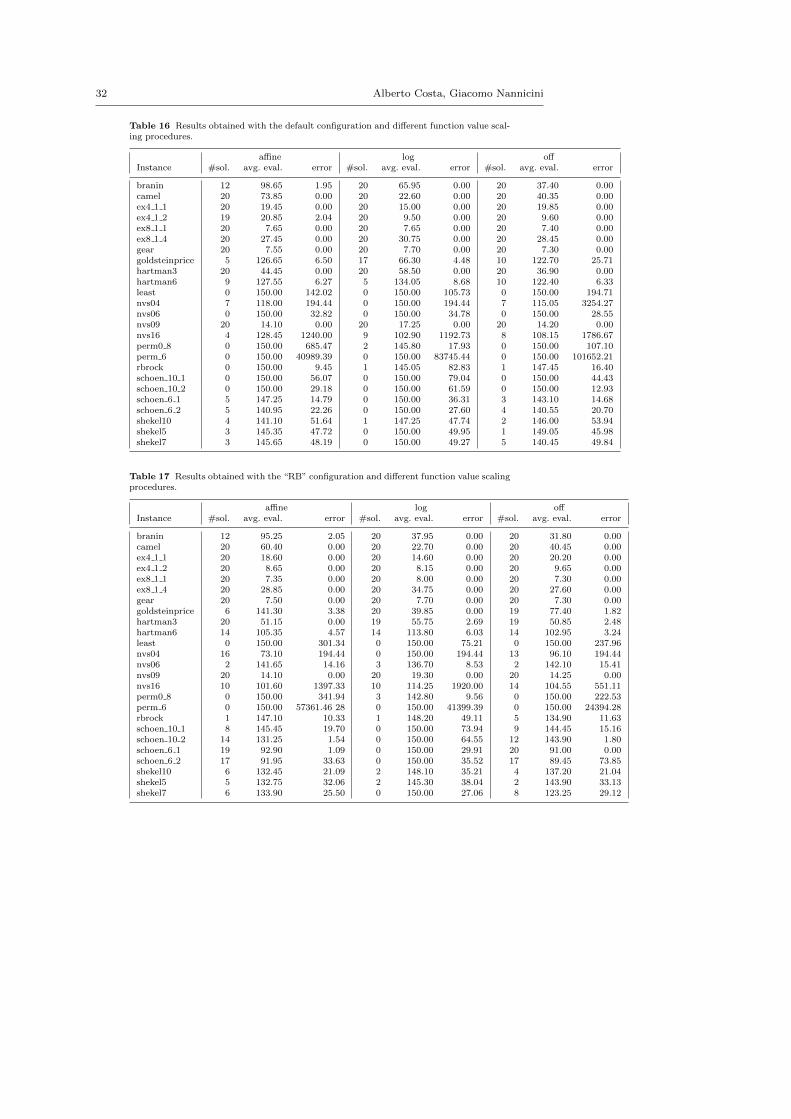
32 Alberto Costa, Giacomo Nannicini
Table 16 Results obtained with the default configuration and different function value scal-ing procedures.
affine log offInstance #sol. avg. eval. error #sol. avg. eval. error #sol. avg. eval. error
branin 12 98.65 1.95 20 65.95 0.00 20 37.40 0.00camel 20 73.85 0.00 20 22.60 0.00 20 40.35 0.00ex4 1 1 20 19.45 0.00 20 15.00 0.00 20 19.85 0.00ex4 1 2 19 20.85 2.04 20 9.50 0.00 20 9.60 0.00ex8 1 1 20 7.65 0.00 20 7.65 0.00 20 7.40 0.00ex8 1 4 20 27.45 0.00 20 30.75 0.00 20 28.45 0.00gear 20 7.55 0.00 20 7.70 0.00 20 7.30 0.00goldsteinprice 5 126.65 6.50 17 66.30 4.48 10 122.70 25.71hartman3 20 44.45 0.00 20 58.50 0.00 20 36.90 0.00hartman6 9 127.55 6.27 5 134.05 8.68 10 122.40 6.33least 0 150.00 142.02 0 150.00 105.73 0 150.00 194.71nvs04 7 118.00 194.44 0 150.00 194.44 7 115.05 3254.27nvs06 0 150.00 32.82 0 150.00 34.78 0 150.00 28.55nvs09 20 14.10 0.00 20 17.25 0.00 20 14.20 0.00nvs16 4 128.45 1240.00 9 102.90 1192.73 8 108.15 1786.67perm0 8 0 150.00 685.47 2 145.80 17.93 0 150.00 107.10perm 6 0 150.00 40989.39 0 150.00 83745.44 0 150.00 101652.21rbrock 0 150.00 9.45 1 145.05 82.83 1 147.45 16.40schoen 10 1 0 150.00 56.07 0 150.00 79.04 0 150.00 44.43schoen 10 2 0 150.00 29.18 0 150.00 61.59 0 150.00 12.93schoen 6 1 5 147.25 14.79 0 150.00 36.31 3 143.10 14.68schoen 6 2 5 140.95 22.26 0 150.00 27.60 4 140.55 20.70shekel10 4 141.10 51.64 1 147.25 47.74 2 146.00 53.94shekel5 3 145.35 47.72 0 150.00 49.95 1 149.05 45.98shekel7 3 145.65 48.19 0 150.00 49.27 5 140.45 49.84
Table 17 Results obtained with the “RB” configuration and different function value scalingprocedures.
affine log offInstance #sol. avg. eval. error #sol. avg. eval. error #sol. avg. eval. error
branin 12 95.25 2.05 20 37.95 0.00 20 31.80 0.00camel 20 60.40 0.00 20 22.70 0.00 20 40.45 0.00ex4 1 1 20 18.60 0.00 20 14.60 0.00 20 20.20 0.00ex4 1 2 20 8.65 0.00 20 8.15 0.00 20 9.65 0.00ex8 1 1 20 7.35 0.00 20 8.00 0.00 20 7.30 0.00ex8 1 4 20 28.85 0.00 20 34.75 0.00 20 27.60 0.00gear 20 7.50 0.00 20 7.70 0.00 20 7.30 0.00goldsteinprice 6 141.30 3.38 20 39.85 0.00 19 77.40 1.82hartman3 20 51.15 0.00 19 55.75 2.69 19 50.85 2.48hartman6 14 105.35 4.57 14 113.80 6.03 14 102.95 3.24least 0 150.00 301.34 0 150.00 75.21 0 150.00 237.96nvs04 16 73.10 194.44 0 150.00 194.44 13 96.10 194.44nvs06 2 141.65 14.16 3 136.70 8.53 2 142.10 15.41nvs09 20 14.10 0.00 20 19.30 0.00 20 14.25 0.00nvs16 10 101.60 1397.33 10 114.25 1920.00 14 104.55 551.11perm0 8 0 150.00 341.94 3 142.80 9.56 0 150.00 222.53perm 6 0 150.00 57361.46 28 0 150.00 41399.39 0 150.00 24394.28rbrock 1 147.10 10.33 1 148.20 49.11 5 134.90 11.63schoen 10 1 8 145.45 19.70 0 150.00 73.94 9 144.45 15.16schoen 10 2 14 131.25 1.54 0 150.00 64.55 12 143.90 1.80schoen 6 1 19 92.90 1.09 0 150.00 29.91 20 91.00 0.00schoen 6 2 17 91.95 33.63 0 150.00 35.52 17 89.45 73.85shekel10 6 132.45 21.09 2 148.10 35.21 4 137.20 21.04shekel5 5 132.75 32.06 2 145.30 38.04 2 143.90 33.13shekel7 6 133.90 25.50 0 150.00 27.06 8 123.25 29.12
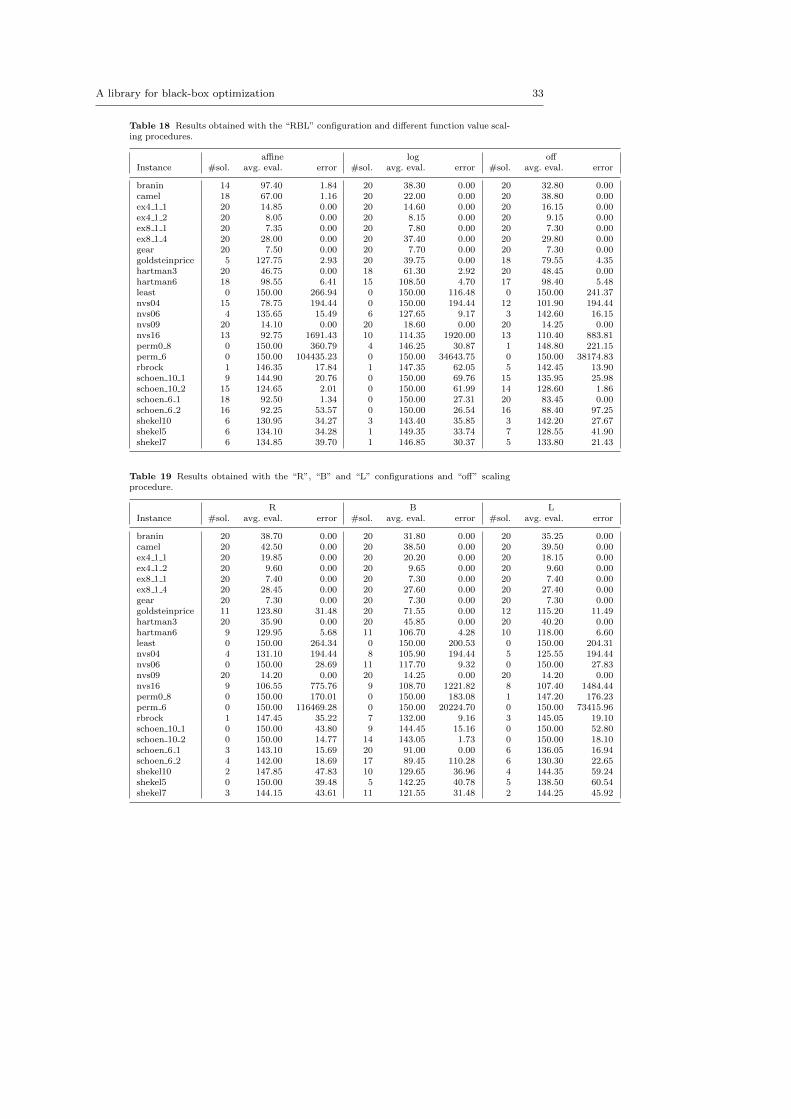
A library for black-box optimization 33
Table 18 Results obtained with the “RBL” configuration and different function value scal-ing procedures.
affine log offInstance #sol. avg. eval. error #sol. avg. eval. error #sol. avg. eval. error
branin 14 97.40 1.84 20 38.30 0.00 20 32.80 0.00camel 18 67.00 1.16 20 22.00 0.00 20 38.80 0.00ex4 1 1 20 14.85 0.00 20 14.60 0.00 20 16.15 0.00ex4 1 2 20 8.05 0.00 20 8.15 0.00 20 9.15 0.00ex8 1 1 20 7.35 0.00 20 7.80 0.00 20 7.30 0.00ex8 1 4 20 28.00 0.00 20 37.40 0.00 20 29.80 0.00gear 20 7.50 0.00 20 7.70 0.00 20 7.30 0.00goldsteinprice 5 127.75 2.93 20 39.75 0.00 18 79.55 4.35hartman3 20 46.75 0.00 18 61.30 2.92 20 48.45 0.00hartman6 18 98.55 6.41 15 108.50 4.70 17 98.40 5.48least 0 150.00 266.94 0 150.00 116.48 0 150.00 241.37nvs04 15 78.75 194.44 0 150.00 194.44 12 101.90 194.44nvs06 4 135.65 15.49 6 127.65 9.17 3 142.60 16.15nvs09 20 14.10 0.00 20 18.60 0.00 20 14.25 0.00nvs16 13 92.75 1691.43 10 114.35 1920.00 13 110.40 883.81perm0 8 0 150.00 360.79 4 146.25 30.87 1 148.80 221.15perm 6 0 150.00 104435.23 0 150.00 34643.75 0 150.00 38174.83rbrock 1 146.35 17.84 1 147.35 62.05 5 142.45 13.90schoen 10 1 9 144.90 20.76 0 150.00 69.76 15 135.95 25.98schoen 10 2 15 124.65 2.01 0 150.00 61.99 14 128.60 1.86schoen 6 1 18 92.50 1.34 0 150.00 27.31 20 83.45 0.00schoen 6 2 16 92.25 53.57 0 150.00 26.54 16 88.40 97.25shekel10 6 130.95 34.27 3 143.40 35.85 3 142.20 27.67shekel5 6 134.10 34.28 1 149.35 33.74 7 128.55 41.90shekel7 6 134.85 39.70 1 146.85 30.37 5 133.80 21.43
Table 19 Results obtained with the “R”, “B” and “L” configurations and “off” scalingprocedure.
R B LInstance #sol. avg. eval. error #sol. avg. eval. error #sol. avg. eval. error
branin 20 38.70 0.00 20 31.80 0.00 20 35.25 0.00camel 20 42.50 0.00 20 38.50 0.00 20 39.50 0.00ex4 1 1 20 19.85 0.00 20 20.20 0.00 20 18.15 0.00ex4 1 2 20 9.60 0.00 20 9.65 0.00 20 9.60 0.00ex8 1 1 20 7.40 0.00 20 7.30 0.00 20 7.40 0.00ex8 1 4 20 28.45 0.00 20 27.60 0.00 20 27.40 0.00gear 20 7.30 0.00 20 7.30 0.00 20 7.30 0.00goldsteinprice 11 123.80 31.48 20 71.55 0.00 12 115.20 11.49hartman3 20 35.90 0.00 20 45.85 0.00 20 40.20 0.00hartman6 9 129.95 5.68 11 106.70 4.28 10 118.00 6.60least 0 150.00 264.34 0 150.00 200.53 0 150.00 204.31nvs04 4 131.10 194.44 8 105.90 194.44 5 125.55 194.44nvs06 0 150.00 28.69 11 117.70 9.32 0 150.00 27.83nvs09 20 14.20 0.00 20 14.25 0.00 20 14.20 0.00nvs16 9 106.55 775.76 9 108.70 1221.82 8 107.40 1484.44perm0 8 0 150.00 170.01 0 150.00 183.08 1 147.20 176.23perm 6 0 150.00 116469.28 0 150.00 20224.70 0 150.00 73415.96rbrock 1 147.45 35.22 7 132.00 9.16 3 145.05 19.10schoen 10 1 0 150.00 43.80 9 144.45 15.16 0 150.00 52.80schoen 10 2 0 150.00 14.77 14 143.05 1.73 0 150.00 18.10schoen 6 1 3 143.10 15.69 20 91.00 0.00 6 136.05 16.94schoen 6 2 4 142.00 18.69 17 89.45 110.28 6 130.30 22.65shekel10 2 147.85 47.83 10 129.65 36.96 4 144.35 59.24shekel5 0 150.00 39.48 5 142.25 40.78 5 138.50 60.54shekel7 3 144.15 43.61 11 121.55 31.48 2 144.25 45.92

34 Alberto Costa, Giacomo Nannicini
Table 20 Results obtained with the “RL” and “BL” configurations and “off” scaling pro-cedure.
RL BLInstance #sol. avg. eval. error #sol. avg. eval. error
branin 20 35.25 0.00 20 32.80 0.00camel 20 39.50 0.00 20 36.90 0.00ex4 1 1 20 18.15 0.00 20 16.15 0.00ex4 1 2 20 9.60 0.00 20 9.15 0.00ex8 1 1 20 7.40 0.00 20 7.30 0.00ex8 1 4 20 27.40 0.00 20 29.80 0.00gear 20 7.30 0.00 20 7.30 0.00goldsteinprice 9 125.05 6.39 18 77.70 3.74hartman3 20 41.35 0.00 20 46.05 0.00hartman6 11 116.90 3.99 11 104.15 4.30least 0 150.00 271.77 0 150.00 213.07nvs04 5 138.50 194.44 7 112.90 194.44nvs06 0 150.00 24.66 6 133.95 8.58nvs09 20 14.20 0.00 20 14.25 0.00nvs16 11 104.60 675.56 8 113.55 1013.33perm0 8 1 147.20 201.63 1 148.80 147.19perm 6 0 150.00 163072.95 0 150.00 24567.01rbrock 2 148.85 35.28 7 135.20 10.72schoen 10 1 0 150.00 52.96 15 135.95 25.98schoen 10 2 0 150.00 19.02 16 127.15 2.25schoen 6 1 6 136.05 17.90 20 83.45 0.00schoen 6 2 6 130.30 17.39 16 88.40 110.26shekel10 2 145.70 49.02 8 136.15 47.75shekel5 5 138.50 56.27 8 127.75 46.82shekel7 2 144.25 41.60 9 127.95 29.08
Table 21 Results obtained with the “RBL” configuration using a noisy oracle with 10% or20% relative error.
RBL n10% RBL n20%Instance #sol. avg. eval. error #sol. avg. eval. error
branin 20 15.27 0.00 20 17.05 0.00camel 20 16.67 0.00 20 16.83 0.00ex4 1 1 20 8.62 0.00 20 9.70 0.00ex4 1 2 20 4.78 0.00 20 5.38 0.00ex8 1 1 20 4.63 0.00 20 6.17 0.00ex8 1 4 20 9.85 0.00 20 10.37 0.00gear 20 3.92 0.00 20 3.87 0.00goldsteinprice 20 36.73 0.00 20 36.87 0.00hartman3 20 28.25 0.00 20 29.32 0.00hartman6 17 67.15 4.96 16 78.55 3.77least 0 150.00 213.58 0 150.00 244.60nvs04 13 70.72 205.62 14 68.48 214.09nvs06 1 146.82 15.95 4 128.67 15.73nvs09 20 5.67 0.00 20 7.35 0.00nvs16 18 42.58 1114.05 16 54.25 1050.43perm0 8 0 150.00 193.64 0 150.00 138.00perm 6 0 150.00 46107.10 0 150.00 35623.78rbrock 4 131.08 15.59 4 126.13 19.37schoen 10 1 3 142.47 33.62 1 147.15 91.73schoen 10 2 7 128.25 6.04 2 145.07 19.94schoen 6 1 15 90.62 8.74 15 95.58 21.51schoen 6 2 14 84.08 51.15 15 96.22 8.54shekel10 6 131.88 31.68 3 142.85 38.53shekel5 1 147.13 43.51 2 145.18 44.30shekel7 1 145.50 36.54 1 147.38 43.56
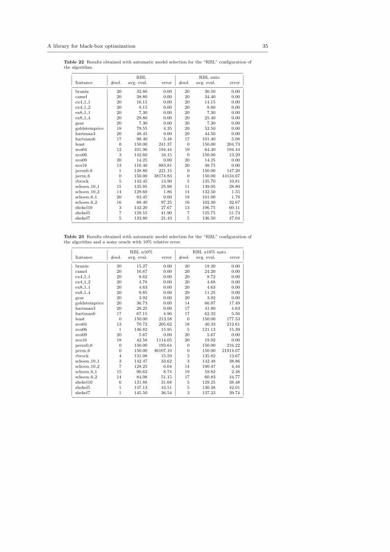
A library for black-box optimization 35
Table 22 Results obtained with automatic model selection for the “RBL” configuration ofthe algorithm.
RBL RBL autoInstance #sol. avg. eval. error #sol. avg. eval. error
branin 20 32.80 0.00 20 30.50 0.00camel 20 38.80 0.00 20 34.40 0.00ex4 1 1 20 16.15 0.00 20 14.15 0.00ex4 1 2 20 9.15 0.00 20 8.60 0.00ex8 1 1 20 7.30 0.00 20 7.30 0.00ex8 1 4 20 29.80 0.00 20 25.40 0.00gear 20 7.30 0.00 20 7.30 0.00goldsteinprice 18 79.55 4.35 20 52.50 0.00hartman3 20 48.45 0.00 20 44.50 0.00hartman6 17 98.40 5.48 17 101.40 5.08least 0 150.00 241.37 0 150.00 204.73nvs04 12 101.90 194.44 19 64.40 194.44nvs06 3 142.60 16.15 0 150.00 13.29nvs09 20 14.25 0.00 20 14.25 0.00nvs16 13 110.40 883.81 20 48.75 0.00perm0 8 1 148.80 221.15 0 150.00 147.20perm 6 0 150.00 38174.83 0 150.00 44134.67rbrock 5 142.45 13.90 5 135.70 10.81schoen 10 1 15 135.95 25.98 11 139.05 28.80schoen 10 2 14 128.60 1.86 14 132.50 1.55schoen 6 1 20 83.45 0.00 18 101.00 1.78schoen 6 2 16 88.40 97.25 16 102.30 32.67shekel10 3 142.20 27.67 13 106.75 60.11shekel5 7 128.55 41.90 7 125.75 51.73shekel7 5 133.80 21.43 5 136.50 47.04
Table 23 Results obtained with automatic model selection for the “RBL” configuration ofthe algorithm and a noisy oracle with 10% relative error.
RBL n10% RBL n10% autoInstance #sol. avg. eval. error #sol. avg. eval. error
branin 20 15.27 0.00 20 18.20 0.00camel 20 16.67 0.00 20 24.20 0.00ex4 1 1 20 8.62 0.00 20 8.72 0.00ex4 1 2 20 4.78 0.00 20 4.68 0.00ex8 1 1 20 4.63 0.00 20 4.63 0.00ex8 1 4 20 9.85 0.00 20 11.25 0.00gear 20 3.92 0.00 20 3.92 0.00goldsteinprice 20 36.73 0.00 14 66.07 17.49hartman3 20 28.25 0.00 17 41.80 4.63hartman6 17 67.15 4.96 17 62.32 5.56least 0 150.00 213.58 0 150.00 177.53nvs04 13 70.72 205.62 18 40.33 212.61nvs06 1 146.82 15.95 5 121.13 15.39nvs09 20 5.67 0.00 20 5.67 0.00nvs16 18 42.58 1114.05 20 19.92 0.00perm0 8 0 150.00 193.64 0 150.00 216.22perm 6 0 150.00 46107.10 0 150.00 21914.07rbrock 4 131.08 15.59 3 135.82 13.67schoen 10 1 3 142.47 33.62 3 142.48 38.86schoen 10 2 7 128.25 6.04 14 100.47 4.44schoen 6 1 15 90.62 8.74 19 59.82 2.48schoen 6 2 14 84.08 51.15 17 60.83 44.77shekel10 6 131.88 31.68 5 129.25 38.48shekel5 1 147.13 43.51 5 130.38 42.01shekel7 1 145.50 36.54 3 137.23 39.74

36 Alberto Costa, Giacomo Nannicini
Table 24 Results obtained with automatic model selection for the “RBL” configuration ofthe algorithm and a noisy oracle with 20% relative error.
RBL n20% RBL n20% autoInstance #sol. avg. eval. error #sol. avg. eval. error
branin 20 17.05 0.00 20 17.78 0.00camel 20 16.83 0.00 20 24.53 0.00ex4 1 1 20 9.70 0.00 20 9.17 0.00ex4 1 2 20 5.38 0.00 20 5.28 0.00ex8 1 1 20 6.17 0.00 20 6.30 0.00ex8 1 4 20 10.37 0.00 20 11.82 0.00gear 20 3.87 0.00 20 3.87 0.00goldsteinprice 20 36.87 0.00 14 81.55 8.04hartman3 20 29.32 0.00 20 33.72 0.00hartman6 16 78.55 3.77 17 80.85 2.82least 0 150.00 244.60 0 150.00 187.66nvs04 14 68.48 214.09 17 41.35 227.86nvs06 4 128.67 15.73 2 141.88 14.61nvs09 20 7.35 0.00 20 7.08 0.00nvs16 16 54.25 1050.43 20 24.33 0.00perm0 8 0 150.00 138.00 0 150.00 233.28perm 6 0 150.00 35623.78 0 150.00 46667.82rbrock 4 126.13 19.37 3 136.97 11.56schoen 10 1 1 147.15 91.73 1 147.75 92.31schoen 10 2 2 145.07 19.94 4 140.13 27.72schoen 6 1 15 95.58 21.51 17 90.15 9.95schoen 6 2 15 96.22 8.54 15 87.05 38.02shekel10 3 142.85 38.53 4 139.50 40.64shekel5 2 145.18 44.30 4 139.05 50.50shekel7 1 147.38 43.56 5 132.70 54.83
Table 25 Results obtained with the “RBL” configuration and “off” scaling procedures anda noisy oracle with 10% relative error, but relative error estimate εr of the algorithm set at20%, and with 20% relative error but relative error estimate εr set at 30%.
RBL n10% (εr = 20%) RBL n20% (εr = 30%)Instance #sol. avg. eval. error #sol. avg. eval. error
branin 20 17.70 0.00 20 17.40 0.00camel 20 16.22 0.00 20 20.32 0.00ex4 1 1 20 9.37 0.00 20 9.98 0.00ex4 1 2 20 5.10 0.00 20 5.18 0.00ex8 1 1 20 5.02 0.00 20 5.78 0.00ex8 1 4 20 10.57 0.00 20 10.32 0.00gear 20 4.05 0.00 20 3.75 0.00goldsteinprice 18 40.78 1.59 18 41.83 14.63hartman3 20 28.42 0.00 20 24.02 0.00hartman6 19 63.47 6.49 15 78.87 3.81least 0 150.00 210.17 1 145.67 231.35nvs04 18 50.45 239.58 13 89.67 243.78nvs06 1 146.55 16.24 5 126.83 6.36nvs09 20 6.40 0.00 20 6.05 0.00nvs16 20 30.52 0.00 20 19.60 0.00perm0 8 1 145.82 175.63 1 148.12 115.15perm 6 0 150.00 21109.16 0 150.00 68840.79rbrock 3 138.22 14.23 4 130.48 28.16schoen 10 1 2 145.35 52.51 1 147.85 81.46schoen 10 2 5 136.15 21.75 3 141.90 27.15schoen 6 1 14 96.63 17.81 6 131.88 27.13schoen 6 2 14 89.97 38.24 14 97.67 24.28shekel10 1 146.55 53.14 6 133.03 35.57shekel5 1 147.50 52.46 2 145.50 41.92shekel7 4 137.03 41.23 3 139.68 56.29


![arXiv:1708.03684v2 [cs.DM] 1 Oct 2017 Introduction to Quantum Computing, Without the Physics Giacomo Nannicini IBM T.J. Watson, Yorktown Heights, NY nannicini@us.ibm.com Last updated:](https://img.dokumen.tips/doc/110x75/5aed28bb7f8b9a585f8fd3da/arxiv170803684v2-csdm-1-oct-2017-introduction-to-quantum-computing-without.jpg)