CHAPTER 1 Tutorial

This chapter gives a short overview of the interpretation of seismic refraction traveltime data with RayfractTM. For more detailed instruc-tions, please refer to the online help and tutorials as available on our web site.

Copyright © 1996-2006 Intelligent Resources Inc. All rights reserved.

Table of Contents

Rayfract Manual 1

CHAPTER 1 TutorialCreate new profile ...............................................................................2Seismic data import .............................................................................3Review first breaks ..............................................................................4Smooth inversion.................................................................................5Automatic refractor mapping ..............................................................6Wavefront method ...............................................................................7Automatic picking ...............................................................................8Manual refractor mapping ...................................................................9Wavefront LINE14 ............................................................................10Wavefront PALMFIG4 ...................................................................... 11ASCII data import .............................................................................12Refractor mapping TRA02ASC ........................................................13Wavefront TRA02ASC .....................................................................14Smooth inversion TRA02ASC ..........................................................15Wavepath coverage............................................................................16Forward model first breaks................................................................17

Tutorial - Create new profile

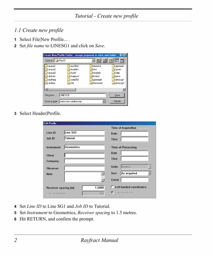
1.1 Create new profile1 Select File|New Profile... . 2 Set file name to LINESG1 and click on Save.

3 Select Header|Profile.

4 Set Line ID to Line SG1 and Job ID to Tutorial.5 Set Instrument to Geometrics, Receiver spacing to 1.5 metres.6 Hit RETURN, and confirm the prompt.

2 Rayfract Manual

Tutorial - Seismic data import

1.2 Seismic data importYour software supports the import of both binary trace data and ASCII formatted files with first breaks and recording geometry, as generated with popular third-party packages. We use the sample W_GeoSoft WinSism file JENNYSG1.XYZ to get you started.

1 Download http://rayfract.com/samples/JENNYSG1.ZIP into a temporary directory.2 Copy JENNYSG1.ZIP into directory \RAY32\JENNYSG1\INUT and unzip it.3 Select File|Import Data to obtain a dialog as shown here :

4 Set Import data type to W_GeoSoft WinSism .XYZ. 5 Click Select, select file JENNYSG1.XYZ in \RAY32\JENNYSG1\INPUT, click Open.6 Set Default shot hole depth to 0.5 metres.7 Set Default spread type to 02: 48 channels.8 Click on Import shots, and confirm the prompt.9 If required, edit Shot pos., Layout start etc. in the following dialog. See above at right.10 Click on Read for all shots as displayed in that dialog, once you have edited these values.11 Click on Skip for shots which you do not want to import at this time, in the same dialog.

Rayfract Manual 3

Tutorial - Review first breaks

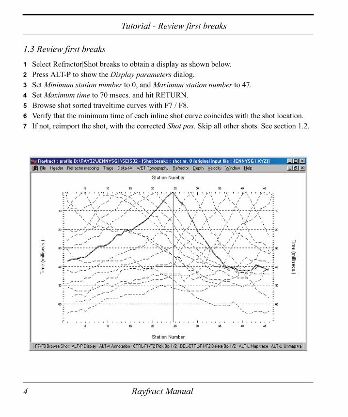
1.3 Review first breaks1 Select Refractor|Shot breaks to obtain a display as shown below.2 Press ALT-P to show the Display parameters dialog.3 Set Minimum station number to 0, and Maximum station number to 47.4 Set Maximum time to 70 msecs. and hit RETURN.5 Browse shot sorted traveltime curves with F7 / F8.6 Verify that the minimum time of each inline shot curve coincides with the shot location.7 If not, reimport the shot, with the corrected Shot pos. Skip all other shots. See section 1.2.

4 Rayfract Manual

Tutorial - Smooth inversion

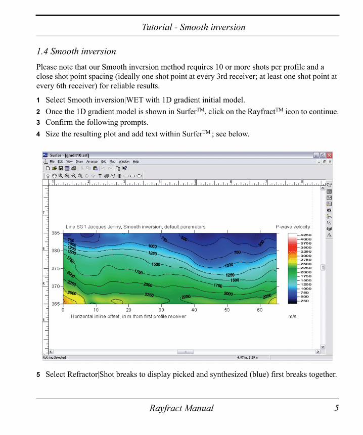
1.4 Smooth inversionPlease note that our Smooth inversion method requires 10 or more shots per profile and a close shot point spacing (ideally one shot point at every 3rd receiver; at least one shot point at every 6th receiver) for reliable results.

1 Select Smooth inversion|WET with 1D gradient initial model.2 Once the 1D gradient model is shown in SurferTM, click on the RayfractTM icon to continue.3 Confirm the following prompts.4 Size the resulting plot and add text within SurferTM ; see below.

5 Select Refractor|Shot breaks to display picked and synthesized (blue) first breaks together.

Rayfract Manual 5

Tutorial - Automatic refractor mapping

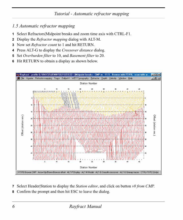
1.5 Automatic refractor mapping1 Select Refractors|Midpoint breaks and zoom time axis with CTRL-F1.2 Display the Refractor mapping dialog with ALT-M. 3 Now set Refractor count to 1 and hit RETURN. 4 Press ALT-G to display the Crossover distance dialog. 5 Set Overburden filter to 10, and Basement filter to 20. 6 Hit RETURN to obtain a display as shown below.

7 Select Header|Station to display the Station editor, and click on button v0 from CMP.8 Confirm the prompt and then hit ESC to leave the dialog.

6 Rayfract Manual

Tutorial - Wavefront method

1.6 Wavefront method1 Select Window|Close All and then Depth|Wavefront.2 Confirm the following prompts.3 Select Depth conversion|Display Wavefront rays.4 Press ALT-P to show the Display parameters dialog.5 Set Minimum station number to 0, and Maximum station number to 47. Hit RETURN.6 Select Velocity|Wavefront. Scale the plot as in previous two steps.7 Select Window|Tile horizontal to obtain a display as shown here :

Rayfract Manual 7

Tutorial - Automatic picking

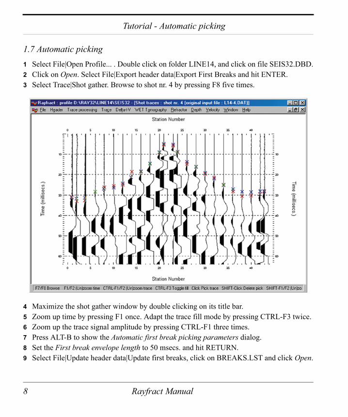
1.7 Automatic picking1 Select File|Open Profile... . Double click on folder LINE14, and click on file SEIS32.DBD.2 Click on Open. Select File|Export header data|Export First Breaks and hit ENTER.3 Select Trace|Shot gather. Browse to shot nr. 4 by pressing F8 five times.

4 Maximize the shot gather window by double clicking on its title bar.5 Zoom up time by pressing F1 once. Adapt the trace fill mode by pressing CTRL-F3 twice.6 Zoom up the trace signal amplitude by pressing CTRL-F1 three times.7 Press ALT-B to show the Automatic first break picking parameters dialog.8 Set the First break envelope length to 50 msecs. and hit RETURN.9 Select File|Update header data|Update first breaks, click on BREAKS.LST and click Open.

8 Rayfract Manual

Tutorial - Manual refractor mapping

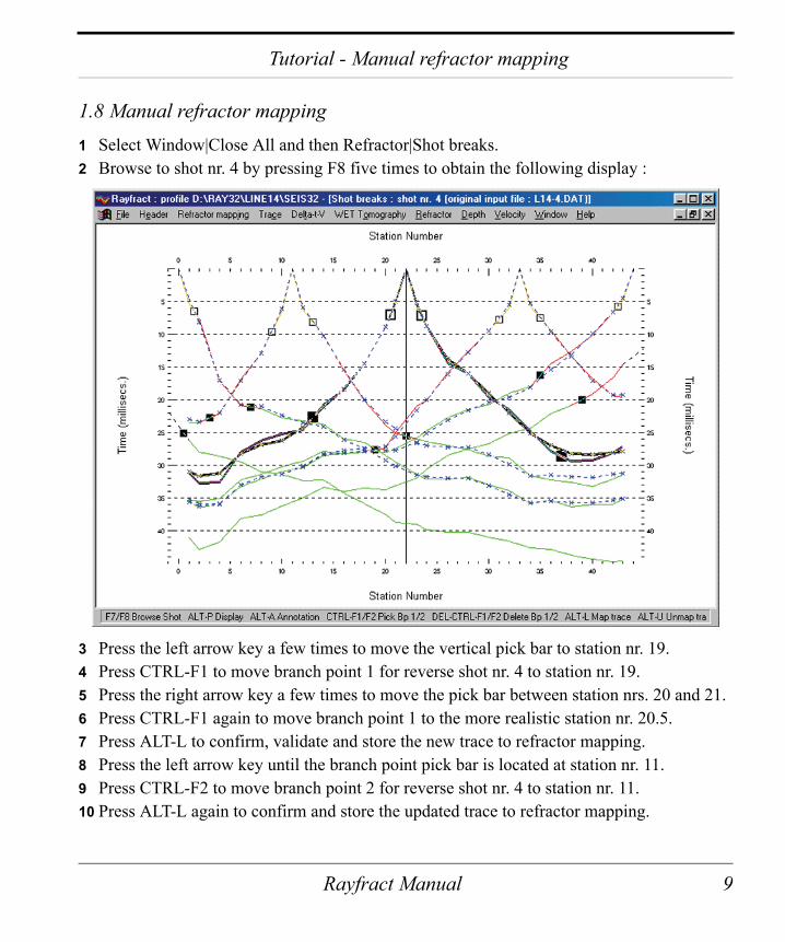
1.8 Manual refractor mapping1 Select Window|Close All and then Refractor|Shot breaks.2 Browse to shot nr. 4 by pressing F8 five times to obtain the following display :

3 Press the left arrow key a few times to move the vertical pick bar to station nr. 19.4 Press CTRL-F1 to move branch point 1 for reverse shot nr. 4 to station nr. 19.5 Press the right arrow key a few times to move the pick bar between station nrs. 20 and 21.6 Press CTRL-F1 again to move branch point 1 to the more realistic station nr. 20.5.7 Press ALT-L to confirm, validate and store the new trace to refractor mapping.8 Press the left arrow key until the branch point pick bar is located at station nr. 11.9 Press CTRL-F2 to move branch point 2 for reverse shot nr. 4 to station nr. 11.10 Press ALT-L again to confirm and store the updated trace to refractor mapping.

Rayfract Manual 9

Tutorial - Wavefront LINE14

1.9 Wavefront LINE141 Select Header|Station to display the Station editor, and click on button v0 from Shots.2 Confirm the prompt and then hit ESC to leave the dialog.3 Select Window|Close All and then Depth|Wavefront. Confirm the following prompts.4 Select Depth conversion|Display Wavefront rays.5 Scale the Wavefront depth and Wavefront velocity sections as described in section 1.6.6 Select Window|Tile horizontal to obtain a display as shown here :

Our Wavefront method is a ray inversion method based on publications by E. Brueckl 1987, and Glyn M. Jones and D. B. Jovanovich 1985. We support modeling of one or two refractors.

10 Rayfract Manual

Tutorial - Wavefront PALMFIG4

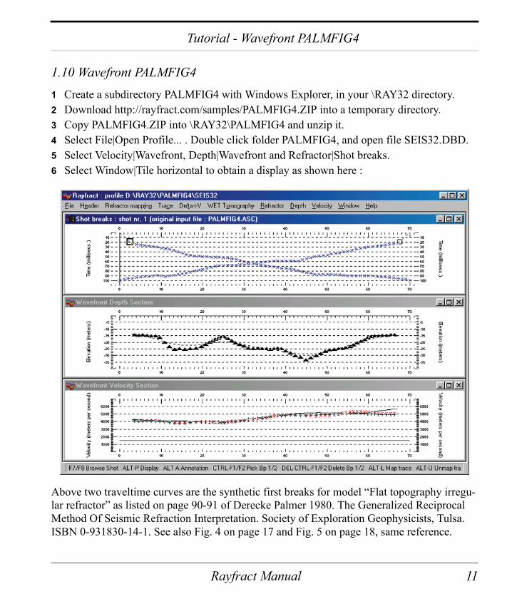
1.10 Wavefront PALMFIG41 Create a subdirectory PALMFIG4 with Windows Explorer, in your \RAY32 directory.2 Download http://rayfract.com/samples/PALMFIG4.ZIP into a temporary directory.3 Copy PALMFIG4.ZIP into \RAY32\PALMFIG4 and unzip it.4 Select File|Open Profile... . Double click folder PALMFIG4, and open file SEIS32.DBD.5 Select Velocity|Wavefront, Depth|Wavefront and Refractor|Shot breaks.6 Select Window|Tile horizontal to obtain a display as shown here :

Above two traveltime curves are the synthetic first breaks for model “Flat topography irregu-lar refractor” as listed on page 90-91 of Derecke Palmer 1980. The Generalized Reciprocal Method Of Seismic Refraction Interpretation. Society of Exploration Geophysicists, Tulsa. ISBN 0-931830-14-1. See also Fig. 4 on page 17 and Fig. 5 on page 18, same reference.

Rayfract Manual 11

Tutorial - ASCII data import

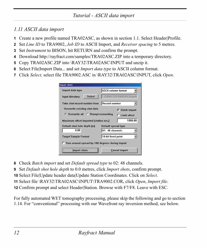
1.11 ASCII data import1 Create a new profile named TRA02ASC, as shown in section 1.1. Select Header|Profile.2 Set Line ID to TRA9002, Job ID to ASCII Import, and Receiver spacing to 5 metres.3 Set Instrument to BISON, hit RETURN and confirm the prompt.4 Download http://rayfract.com/samples/TRA02ASC.ZIP into a temporary directory.5 Copy TRA02ASC.ZIP into \RAY32\TRA02ASC\INPUT and unzip it.6 Select File|Import Data... and set Import data type to ASCII column format.7 Click Select, select file TRA9002.ASC in \RAY32\TRA02ASC\INPUT, click Open.

8 Check Batch import and set Default spread type to 02: 48 channels.9 Set Default shot hole depth to 0.0 metres, click Import shots, confirm prompt.10 Select File|Update header data|Update Station Coordinates. Click on Select.11 Select file \RAY32\TRA02ASC\INPUT\TRA9002.COR, click Open, Import file.12 Confirm prompt and select Header|Station. Browse with F7/F8. Leave with ESC.

For fully automated WET tomography processing, please skip the following and go to section 1.14. For “conventional” processing with our Wavefront ray inversion method, see below.

12 Rayfract Manual

Tutorial - Refractor mapping TRA02ASC

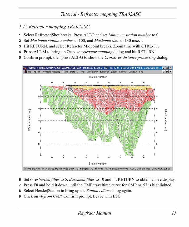
1.12 Refractor mapping TRA02ASC1 Select Refractor|Shot breaks. Press ALT-P and set Minimum station number to 0.2 Set Maximum station number to 100, and Maximum time to 130 msecs.3 Hit RETURN. and select Refractor|Midpoint breaks. Zoom time with CTRL-F1.4 Press ALT-M to bring up Trace to refractor mapping dialog and hit RETURN.5 Confirm prompt, then press ALT-G to show the Crossover distance processing dialog.

6 Set Overburden filter to 5, Basement filter to 10 and hit RETURN to obtain above display.7 Press F8 and hold it down until the CMP traveltime curve for CMP nr. 57 is highlighted.8 Select Header|Station to bring up the Station editor dialog again.9 Click on v0 from CMP. Confirm prompt. Leave with ESC.

Rayfract Manual 13

Tutorial - Wavefront TRA02ASC

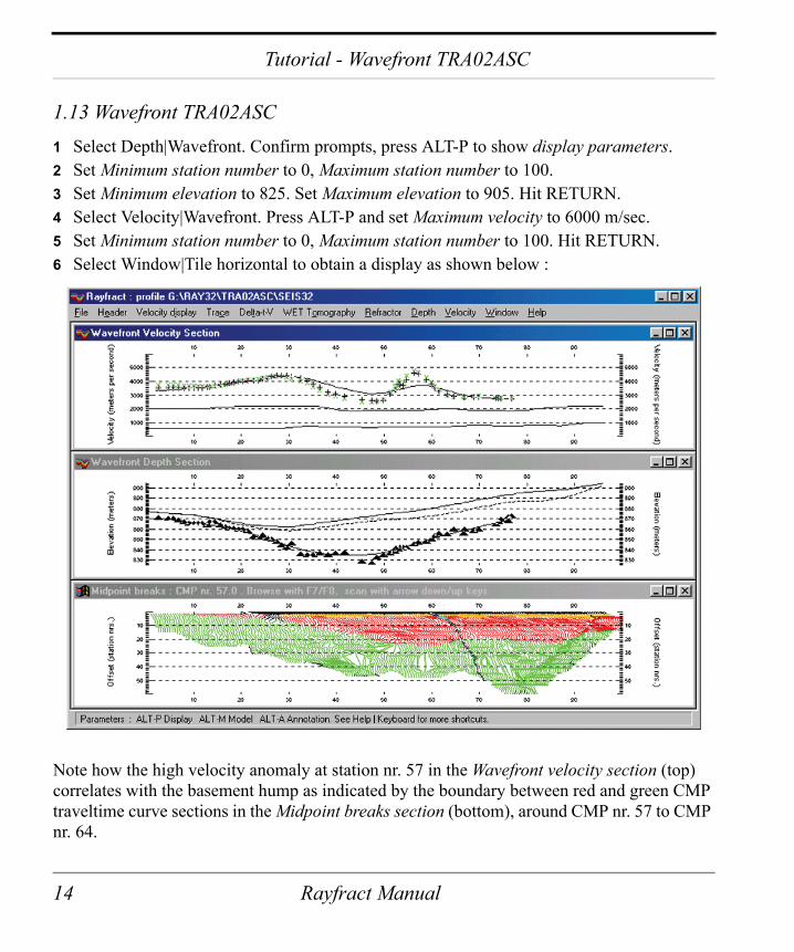
1.13 Wavefront TRA02ASC1 Select Depth|Wavefront. Confirm prompts, press ALT-P to show display parameters.2 Set Minimum station number to 0, Maximum station number to 100.3 Set Minimum elevation to 825. Set Maximum elevation to 905. Hit RETURN.4 Select Velocity|Wavefront. Press ALT-P and set Maximum velocity to 6000 m/sec.5 Set Minimum station number to 0, Maximum station number to 100. Hit RETURN.6 Select Window|Tile horizontal to obtain a display as shown below :

Note how the high velocity anomaly at station nr. 57 in the Wavefront velocity section (top) correlates with the basement hump as indicated by the boundary between red and green CMP traveltime curve sections in the Midpoint breaks section (bottom), around CMP nr. 57 to CMP nr. 64.

14 Rayfract Manual

Tutorial - Smooth inversion TRA02ASC

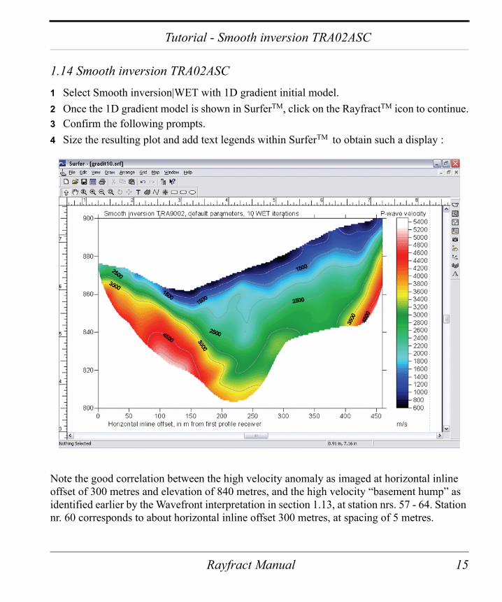
1.14 Smooth inversion TRA02ASC1 Select Smooth inversion|WET with 1D gradient initial model.2 Once the 1D gradient model is shown in SurferTM, click on the RayfractTM icon to continue.3 Confirm the following prompts.4 Size the resulting plot and add text legends within SurferTM to obtain such a display :

Note the good correlation between the high velocity anomaly as imaged at horizontal inline offset of 300 metres and elevation of 840 metres, and the high velocity “basement hump” as identified earlier by the Wavefront interpretation in section 1.13, at station nrs. 57 - 64. Station nr. 60 corresponds to about horizontal inline offset 300 metres, at spacing of 5 metres.

Rayfract Manual 15

Tutorial - Wavepath coverage

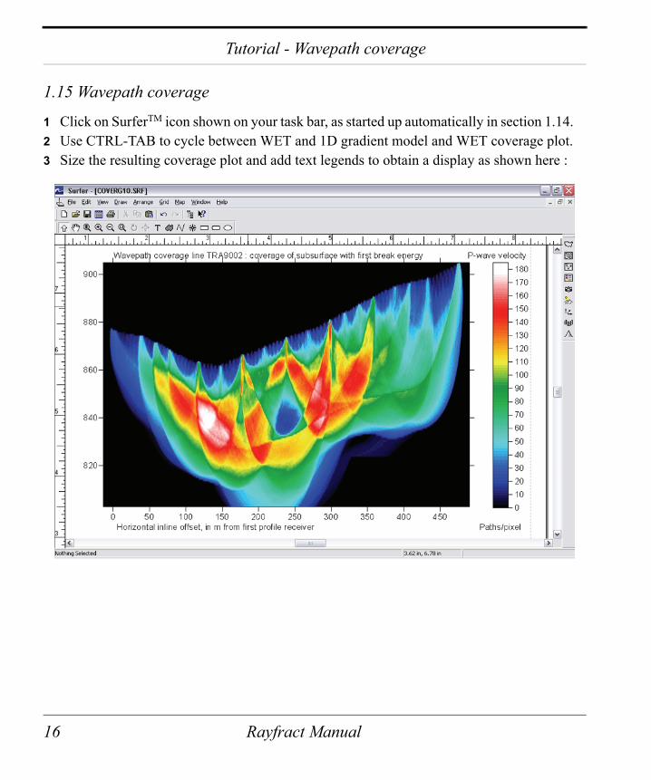
1.15 Wavepath coverage

1 Click on SurferTM icon shown on your task bar, as started up automatically in section 1.14.

2 Use CTRL-TAB to cycle between WET and 1D gradient model and WET coverage plot.3 Size the resulting coverage plot and add text legends to obtain a display as shown here :

16 Rayfract Manual

Tutorial - Forward model first breaks

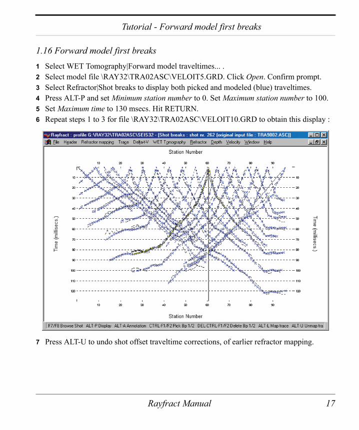
1.16 Forward model first breaks1 Select WET Tomography|Forward model traveltimes... .2 Select model file \RAY32\TRA02ASC\VELOIT5.GRD. Click Open. Confirm prompt.3 Select Refractor|Shot breaks to display both picked and modeled (blue) traveltimes.4 Press ALT-P and set Minimum station number to 0. Set Maximum station number to 100.5 Set Maximum time to 130 msecs. Hit RETURN.6 Repeat steps 1 to 3 for file \RAY32\TRA02ASC\VELOIT10.GRD to obtain this display :

7 Press ALT-U to undo shot offset traveltime corrections, of earlier refractor mapping.

Rayfract Manual 17