University of Applied Sciences Basel (FHBB)Diploma Thesis

DA07 0405 RayTracing on GPU

Ray Tracing on GPU

Martin Christenmartin.christen@stud.fhbb.ch

January 19, 2005

Assistant Professor: Marcus HudritschSupervisor: Wolfgang Engel

Abstract

In this paper I present a way to implement Whitted style (“classic”) recursive raytracing on current generation consumer level GPUs using the OpenGL ShadingLanguage (GLSL) and the Direct3D High Level Shading Language (HLSL). Ray trac-ing is implemented using a simplified, abstracted stream programming model forthe GPU, written in C++.

A ray tracer on current graphics hardware reaches the speed of a good CPUimplementation already. Combined with classic triangle based real time rendering,the GPU based ray tracing algorithm could already be used today for certain specialeffects in computer games.

2

Contents

1. Introduction 5

2. Introduction to Ray Tracing 62.1. What is Ray Tracing ? . . . . . . . . . . . . . . . . . . . . . . . . . . . . . 62.2. Simple Ray Tracing Implementation . . . . . . . . . . . . . . . . . . . . 72.3. Accelerating Ray Tracing . . . . . . . . . . . . . . . . . . . . . . . . . . . 8

2.3.1. Using Spatial Data Structures . . . . . . . . . . . . . . . . . . . . 82.3.2. Eliminating Recursion . . . . . . . . . . . . . . . . . . . . . . . . . 8

3. GPU Programming 93.1. Programmable Graphics Hardware Pipeline . . . . . . . . . . . . . . . . 9

3.1.1. Programmable Vertex Processor . . . . . . . . . . . . . . . . . . . 103.1.2. Primitive Assembly and rasterization . . . . . . . . . . . . . . . . 103.1.3. Programmable Fragment Processor . . . . . . . . . . . . . . . . . 103.1.4. Raster Operations . . . . . . . . . . . . . . . . . . . . . . . . . . . 11

3.2. Examples of Common Shader Applications . . . . . . . . . . . . . . . . 113.2.1. Advanced Lighting Model . . . . . . . . . . . . . . . . . . . . . . . 113.2.2. Bump Mapping . . . . . . . . . . . . . . . . . . . . . . . . . . . . . 123.2.3. Non Photorealistic Rendering . . . . . . . . . . . . . . . . . . . . . 12

4. Stream Programming on GPU 134.1. Streaming Model for GPUs . . . . . . . . . . . . . . . . . . . . . . . . . . 13

4.1.1. Definitions . . . . . . . . . . . . . . . . . . . . . . . . . . . . . . . 134.1.2. Implementing the Model on GPU . . . . . . . . . . . . . . . . . . . 14

4.2. C++ Implementation . . . . . . . . . . . . . . . . . . . . . . . . . . . . . . 154.2.1. Kernel and Array Definition . . . . . . . . . . . . . . . . . . . . . . 154.2.2. Loops and Termination Conditions . . . . . . . . . . . . . . . . . 16

4.3. Kernel Chains . . . . . . . . . . . . . . . . . . . . . . . . . . . . . . . . . 174.3.1. Sequence . . . . . . . . . . . . . . . . . . . . . . . . . . . . . . . . 174.3.2. For-loop . . . . . . . . . . . . . . . . . . . . . . . . . . . . . . . . . 174.3.3. While Loop over one kernel . . . . . . . . . . . . . . . . . . . . . . 184.3.4. While-Loop over several kernels . . . . . . . . . . . . . . . . . . . 18

3

4.3.5. Nested-While-Loop . . . . . . . . . . . . . . . . . . . . . . . . . . . 19

5. Ray Tracing on GPU 205.1. Choosing the Acceleration Structure . . . . . . . . . . . . . . . . . . . . 20

5.1.1. Creating the Uniform Grid . . . . . . . . . . . . . . . . . . . . . . 215.1.2. Traversing the Uniform Grid . . . . . . . . . . . . . . . . . . . . . 21

5.2. Removing Recursion . . . . . . . . . . . . . . . . . . . . . . . . . . . . . . 255.2.1. Reflection . . . . . . . . . . . . . . . . . . . . . . . . . . . . . . . . 255.2.2. Refraction . . . . . . . . . . . . . . . . . . . . . . . . . . . . . . . . 26

5.3. Storing the 3D Scene . . . . . . . . . . . . . . . . . . . . . . . . . . . . . 265.4. Kernels for Ray Tracing . . . . . . . . . . . . . . . . . . . . . . . . . . . . 27

5.4.1. Primary Ray Generator . . . . . . . . . . . . . . . . . . . . . . . . 285.4.2. Voxel Precalculation . . . . . . . . . . . . . . . . . . . . . . . . . . 285.4.3. Ray Traverser . . . . . . . . . . . . . . . . . . . . . . . . . . . . . . 295.4.4. Ray Intersector . . . . . . . . . . . . . . . . . . . . . . . . . . . . . 30

5.5. Early-Z Culling . . . . . . . . . . . . . . . . . . . . . . . . . . . . . . . . . 305.6. Load Balancing Traversing and Intersection Loop . . . . . . . . . . . . . 31

6. Results 336.1. Implementation . . . . . . . . . . . . . . . . . . . . . . . . . . . . . . . . 336.2. Benchmark . . . . . . . . . . . . . . . . . . . . . . . . . . . . . . . . . . . 34

6.2.1. Demo Scenes . . . . . . . . . . . . . . . . . . . . . . . . . . . . . . 346.2.2. Result: GPU . . . . . . . . . . . . . . . . . . . . . . . . . . . . . . . 376.2.3. Result: GPU vs. CPU . . . . . . . . . . . . . . . . . . . . . . . . . 38

6.3. Observations . . . . . . . . . . . . . . . . . . . . . . . . . . . . . . . . . . 396.4. Possible Future Improvements . . . . . . . . . . . . . . . . . . . . . . . . 39

7. Conclusion 40

A. Screenshots 41

Bibliography 43

4

1. Introduction

Today, there are already computer games running in real time raytracing usingclusters of PCs[14]. Now the questions is if future generations of GPUs (GraphicsProcessing Units) will make real time ray tracing possible on single CPU consumercomputers.

Dual GPU solutions are entering the market, NVidia’s SLI1 and it seems Gigabytewill release a dual GPU one-board-solution with 2 GeForce 6600 GT2. There is a lotof promising development from GPU producers.

There have been several approaches to map ray tracing to GPUs. One is theapproach described by Timothy J. Purcell[11], several of his ideas were used forthis project.

The GPU Ray Tracer created for this paper – including the source code – is down-loadable at the project site.3. Be advised that the current version runs on NVidiaGeForce 6 cards only.

1http://www.nvidia.com2 http://www.tomshardware.com/hardnews/20041216 115811.html3http://www.fhbb.ch/informatik/bvmm/

5

2. Introduction to Ray Tracing

2.1. What is Ray Tracing ?

Ray tracing is a method of generating realistic images, in which the paths of indi-vidual rays of light are followed from the viewer to their points of origin.

The core concept of any kind of ray tracing algorithm is to efficiently find inter-sections of a ray with a scene consisting of a set of geometric primitives.

The scene to be rendered consists of a list of geometric primitives, which areusually simple geometric shapes such as as polygons, spheres, cones, etc. In fact,any kind of object can be used as a ray tracing primitive as long as it is possible tocompute an intersection between a ray and the primitive.

eye

Object

primary ray

Figure 2.1.: Ray Tracing: Basic Concept

However, supporting triangles only[15] makes it easier to write, maintain, andoptimize the ray tracer, and thus greatly simplifies both design and optimized im-plementation. Most scenes usually contain few “perfect spheres” or other high-levelprimitives. Furthermore most programs in the industry are exclusively based ontriangular meshes.

Supporting triangles only does not really limit the kinds of scenes to be ren-dered, since all of these high-level primitives can usually be well approximated bytriangles.

6

2.2. Simple Ray Tracing Implementation

Turner Whitted[16] introduced a simple way to ray trace recursively.� �RayRender{

for each pixel x ,y{

calculatePrimaryRay (x ,y ,ray ) ; // Ray originating from thecamera/eye

color = RayTrace (ray ) ; // Start Recursion for thispixel

writePixel (x ,y ,color ) ; // write Pixel to Output Buffer}

}� �� �Color RayTrace (Ray& ray ){Color = BackgroundColor ;RayIntersect (ray ) ;if (ray .length < INFINITY ){color = RayShade (ray ) ;if (ray .depth < maxDepth && contribution > minContrib ){

if (ObjectIsReflective ( ) ) color += kr ∗ RayTrace (reflected_ray ) ;if (ObjectIsTransparent ( ) ) color += kt ∗ RayTrace (transmitted_ray

) ;}

}return color ;

}� �� �Color RayShade (Ray &ray ){

for all light sources{

shadowRay=GenerateShadowRay (ray , light [i ] ) ;if (shadowRay .length > light_distance ) localColor +=CalcLocalColor ( ) ;

}return localColor ;

}� �

7

2.3. Accelerating Ray Tracing

Ray Tracing is time consuming because of the high number of intersection tests.Each ray has to be checked against all objects in a scene, so the primary approachto accelerate ray tracing is to reduce the total number of hit tests.

2.3.1. Using Spatial Data Structures

Finding the closest object hit by a ray requires the ray to be intersected with theprimitives in the scene. A “brute force” approach of simply intersecting the raywith each geometric primitive is too expensive, therefore, accelerating this processusually involves traversing some form of an acceleration structure - in most casesa spatial data structure - is used to find objects nearby the ray. Spatial data struc-tures are for example bounding volume hierarchies, BSP trees, kd trees, octrees,uniform grids, adaptive grids, hierarchical grids, etc.[2]

2.3.2. Eliminating Recursion

As shown in section 2.1, Ray tracing is usually used in a recursive manner. Inorder to compute the color of primary rays, recursive ray tracing algorithm castsadditional, secondary rays creating indirect effects like shadows, reflection or re-fraction. It is possible to eliminate the need for recursion and to write the raytracer in an iterative way which runs faster since we don’t need function calls andthe stack.

8

3. GPU Programming

3.1. Programmable Graphics Hardware Pipeline

A pipeline is a sequence of steps operating in parallel and in a fixed order. Eachstage receives its input from the prior stage and sends its output to the subsequentstage.

Pretransformed Vertices

ProgrammableVertex Processor

Transformed Vertices

Primitive Assembly

Assembled Polygons,Lines, and Points

Rasterization andInterpolation

RasterizedPretransformedFragments

ProgrammableFragment Processor

Raster Operations

Transformed Fragments

Pixel Updates

Frame Buffer

Early-Z Culling

Figure 3.1.: Simplified Pipeline

9

3.1.1. Programmable Vertex Processor

The vertex processor is a programmable unit that operates on incoming vertex at-tributes, such as position, color, texture coordinates, and so on. The vertex proces-sor is intended to perform traditional graphics operations such as vertex transfor-mation, normal transformation/normalization, texture coordinate generation, andtexture coordinate transformation.

The vertex processor only has one vertex as input and only writes one vertexas output, therefore topological information of the vertices is not available to thevertex processor.

Vertex processing on GPU uses a limited number of mathemathical operationson floating-point vectors (two, three or four components). Operations include add,multiply, multiply-add, dot product, minumum, and maximum. Hardware supportfor vector negation and component-wise swizzling 1 is used to provide negation,subtraction, and cross products. The hardware also adds support for many utilityfunctions like approximations of exponential, logarithmic, and trigonometric func-tions.

3.1.2. Primitive Assembly and rasterization

After vertex processing all vertex attributes are completely determined. The vertexdata is then sent to the stage called Primitive Assembly. At this point vertex data isassembled into complete primitives. Points, lines, triangles, quads etc. may requireclipping to the view frustum or application specified clip planes. The rasterizer mayalso discard polygons that are front or backfacing (culling).

3.1.3. Programmable Fragment Processor

The programmable fragment processor has most of the operations as the program-mable vertex processor provides. In addition the fragment processor requires tex-ture operations to access texture images. On current generation GPUs, floating-point values are supported.

The fragment processor is intended to perform traditional graphics operationssuch as operations on interpolated values, texture access, texture application, fog,and color sum.

To support parallelism at the fragment processing level, fragment programs onlywrite one pixel. Newer GPUs provide multiple rendering target support which allowsto write up to 4 fragments to 4 different render targets in one fragment program.

1Swizzling is the ability to reorder vector components arbitrarily.

10

3.1.4. Raster Operations

Each fragment is checked based on a number of tests, including scissor, alpha,stencil, and depth tests. After those tests a blending operation combines the fi-nal color with the correpsonding pixel’s color value. On newer graphics cardsdepth testing can actually be done before calling the fragment processor (“Early-ZCulling”), and would not execute the fragment program if it is rejected[9]. This isuseful for very long fragment programs.

3.2. Examples of Common Shader Applications

Shader Programs are usually very small programs, mainly used in computer gamesfor special effects. There are many possible applications and only a few are pre-sented here, without going into detail.

3.2.1. Advanced Lighting Model

Figure 3.2.: Cook-Torrance Lighting Model

The processing of every fragment (fragment shader) makes it possible to implement(advanced) lighting models – like the Cook-Torrance lighting model[5] – using a perfragment calculation.

11

3.2.2. Bump Mapping

Figure 3.3.: Bump Mapping

Lighting calculations can be done in a different coordinate system like a TBN(tangent-binormal-normal) orthonormal base (“Texture Space”). This allows to eas-ily implement bump mapping[3] in real time rendering applications.

3.2.3. Non Photorealistic Rendering

Figure 3.4.: Non Photorealisic Rendering - Cartoon Effects

Using tricks, it is possible to add special effects like cartoon-like[6] rendering. Suchrendering is specially used in computer games.

12

4. Stream Programming on GPU

There are several approaches to abstract the GPU to a streaming graphics proces-sor. One such implementation is Brook for GPUs, a compiler and runtime imple-mentation of the brook stream program language[4] for GPUs. Another approachis Sh[8], a metaprogramming language for GPUs, which also has a stream abstrac-tion.

However, the approach used here is to hand-code a general purpose GPU programin GLSL and HLSL with a simple abstracted streaming model controlled in C++.

4.1. Streaming Model for GPUs

Shading languages are different from conventional programming languages. A GPUis not a serial processor, GPUs are based on a dataflow computational model - astreaming model. Computation occurs in response to data that flows through asequence of processing steps. A function is executed on a set of input records(fragments) and outputs a set of output records (pixels). Stream processors typi-cally refer to this function as “Kernel” and to the set of data as a “stream”.

For the ray tracer and for other general purpose programs on GPU, it makessense to abstract words like “fragment” or “pixel” to a higher level name, and tocreate a model to simplify the design of such programs.

4.1.1. Definitions

Stream A stream is a set of data. All data is of the same type. Stream elements canonly be accessed read-only or write-only.

Data Array A data array is a set of data of the same type. Data arrays providerandom access (“Gather”).

Kernel Kernels are small programs operating on streams. Kernels take a stream asinput and produce a stream as ouput. Kernels may also access several staticdata arrays. A kernel is allowed to reject input data and write no output.

13

4.1.2. Implementing the Model on GPU

Stream Streams are floating point textures with render target support.

Data Array data arrays are floating point textures.

Kernel Kernels are fragment shader programs.

A GPU fragment program can read from any location from texures (“gather”), butcannot write to arbitrary global memory (“scatter”). The output of the fragment pro-gram is an image in global memory, with each fragment computation correspondingto a separate pixel in that image. So we have an “input stream” and an “outputstream” to consider. The “output stream” may become an input of another kernel -or for loops an input of the same kernel.

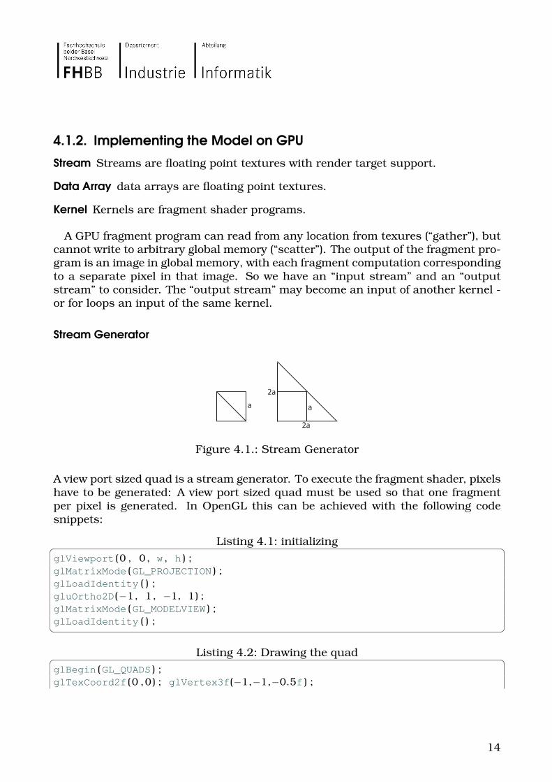
Stream Generator

a a

2a

2a

Figure 4.1.: Stream Generator

A view port sized quad is a stream generator. To execute the fragment shader, pixelshave to be generated: A view port sized quad must be used so that one fragmentper pixel is generated. In OpenGL this can be achieved with the following codesnippets:

Listing 4.1: initializing� �glViewport (0 , 0 , w , h ) ;glMatrixMode (GL_PROJECTION ) ;glLoadIdentity ( ) ;gluOrtho2D(−1, 1 , −1, 1) ;glMatrixMode (GL_MODELVIEW ) ;glLoadIdentity ( ) ;� �

Listing 4.2: Drawing the quad� �glBegin (GL_QUADS ) ;glTexCoord2f (0 ,0) ; glVertex3f(−1,−1,−0.5f ) ;

14

glTexCoord2f (1 ,0) ; glVertex3f ( 1,−1,−0.5f ) ;glTexCoord2f (1 ,1) ; glVertex3f ( 1 , 1,−0.5f ) ;glTexCoord2f (0 ,1) ; glVertex3f(−1, 1,−0.5f ) ;glEnd ( ) ;� �

The quad could also be generated using one triangle only, and adjust the viewportso that only a quad is drawn.

Process Flow of a General purpose GPU program

The usual process flow of a general purpose GPU program is:

1. Draw a quad, texels are mapped to pixels 1:1

2. Run a SIMD program (shader program, kernel) over each fragment

3. Resulting Texture-Buffer (output stream) can be treated as input texture (in-put stream) on the next pass.

4.2. C++ Implementation

4.2.1. Kernel and Array Definition

The C++ implementation uses 3 classes:

GPUStreamGenerator to generate a data stream (i.e. draw a quad).

GPUFloatArray to use as an input- or output-array.

GPUKernel to specifiy a GPU program and add input- and output arrays to it.

Listing 4.3: Example: Kernel and Array Definition� �GPUKernel∗ K = new GPUKernel (shaderFX , "ProgramName" ) ;GPUFloatArray D∗ = new GPUFloatArray (width ,height ,4 ) ;

K−>addInput (D , "VariableName" ) ;K−>addOutput (D ) ;

K−>execute ( ) ; // Start Kernel .� �

15

This example creates one array which will be used as input and output for thekernel. This information has to be set one time and then it is possible to start thekernel with “execute”. Using an Occlusion Query1, the function “execute” returnsthe actual number of values (pixels) written to the output array.

K1

1

Figure 4.2.: Visualisation of a kernel that is called one time

4.2.2. Loops and Termination Conditions

As we saw in last section, it is possible to retrieve the number of values that wereactually written to the output array. This leads to another function, “loop”. IfK->loop() is called, the kernel is executed until no values are written. This isdangerous, because it could lead to an infinte loop, so the kernel requires somesort of termination condition. It is in the response of the kernel programmer totake care of that. n = K->loop() returns the total number of performed kernelcalls.

Listing 4.4: HLSL Example: Termination Condition� �struct pixel{

float4 color : COLOR ;} ;

pixel demo (varying_data IN ){

pixel OUT ;OUT .color = tex2D (tex0 ,IN .texCoord ) ;OUT .color .r += 0.01;if (OUT .color .r >= 1.0) discard ;return OUT ;

}� �In this HLSL example the value of the first component (pixel red component) isincreased by 0.01. If the value reaches 1.0, the fragment is rejected and nothing willbe drawn. Imagine an array full of random values in the range [0, 1]. When you loop

1Occlusion Queries are generally used to enable Occlusion Culling - a technique to accelleraterendering by not rendering hidden objects. In general purpose GPU programming this techniqueis used to count values.

16

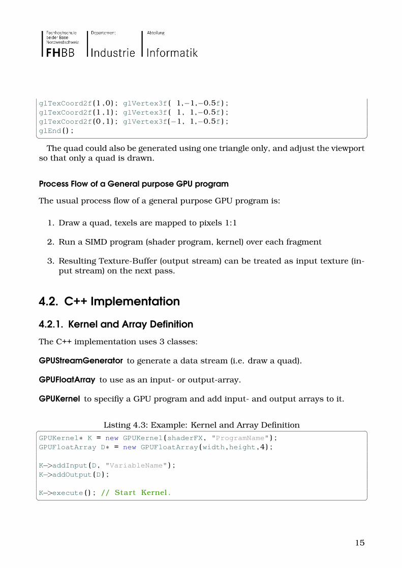
this kernel it will run until all values are 1.0, but there is no way to tell in advancehow many kernel calls are necessary to reach this state.

K1*

Figure 4.3.: Visualisation of a (terminating) kernel which can be used for loops

4.3. Kernel Chains

Kernels can be chained together (sequence) or same Kernels can be called severaltimes, using repetition or loops as shown in 4.2.2.

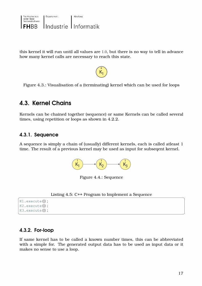
4.3.1. Sequence

A sequence is simply a chain of (usually) different kernels, each is called atleast 1time. The result of a previous kernel may be used as input for subseqent kernel.

K1 K2 K3

1 1 1

Figure 4.4.: Sequence

Listing 4.5: C++ Program to Implement a Sequence� �K1 .execute ( ) ;K2 .execute ( ) ;K3 .execute ( ) ;� �

4.3.2. For-loop

If same kernel has to be called a known number times, this can be abbreviatedwith a simple for. The generated output data has to be used as input data or itmakes no sense to use a loop.

17

K1 K2

115

Figure 4.5.: for

Listing 4.6: C++ Program to Implement a For-Loop� �for (int i=0;i<15;i++) K1 .execute ( ) ;K2 .execute ( ) ;� �4.3.3. While Loop over one kernel

If a kernel has to be looped until its internal termination condition is reached (asshown in 4.2.2) then it can be done using K->loop().

K1 K2* 1

Figure 4.6.: While-Loop over one kernel

Listing 4.7: C++ Program to Implement a While-Loop� �K1 .loop ( ) ;K2 .execute ( ) ;� �4.3.4. While-Loop over several kernels

It is not possible to use loop() if you want to loop over several kernels. Usually the2nd kernel contains the termination condition in this case. This scenario cannotbe reduced to one kernel in general.

K1 K2**

Figure 4.7.: While-Loop over several kernels

18

Listing 4.8: C++ Program to Implement a While-Loop over several kernels� �int n=0;while (n !=1){

n=0;K1 .execute ( ) ;if (K2 .execute ( ) ==0) n++;

}� �4.3.5. Nested-While-Loop

Sometimes loops may be nested, this situation is also easy to implement.

Listing 4.9: C++ Program to Implement a Nested-While-Loop� �int n=0;while (n !=2){

n=0;if (K1 .loop ( ) ==1) n++;if (K2 .loop ( ) ==1) n++;

}� �

19

5. Ray Tracing on GPU

5.1. Choosing the Acceleration Structure

The uniform grid is the easiest spatial data structure to implement on currentgeneration GPUs, because there is minimal data access when traversing it andtraversal is linear. In a uniform grid the scene is uniformly divided into voxelsand those voxels containing triangles or part of a triangle obtain a reference to thistriangle.

Figure 5.1.: Spatial Data Structure: Uniform Grid

20

Figure 5.2.: In the uniform grid, the triangle is referenced in every cell containinga part of the triangle

5.1.1. Creating the Uniform Grid

A simple approach can be used to create the uniform grid.For all triangles Ti in the scene:

1. Calculate the bounding cells (b1, b2) of Triangle Ti

2. Test triangle-box intersection: Ti with every cell Cj ∈ (b1, b2)

3. If triangle-box intersection returned true, add a reference of Ti to Cj.

Figure 5.3.: Scene Converted to Uniform Grid

The uniform grid is generated on CPU and stored in textures. This restricts thecurrent implementation rendering static scenes only. We will learn more aboutstoring data in textures in section 5.3.

5.1.2. Traversing the Uniform Grid

John Amanatides and Andrew Woo[1] presented a way to traverse the grid fastusing a 3D-DDA (digital differential) algorithm. With slight modifications, this al-gorithm can be mapped to the GPU.

21

Figure 5.4.: Traversing Uniform Grid using a 3D-DDA Algorithm

Because it is a very important algorithm for this approach of the ray tracer, itis explained in detail, including full source code (which is missing in the originalpaper of Amanatides/Woo).

The algorithm consists of two steps: initialization and incremental traversal.

Initialization

During the initialization the voxel-position of the origin of the ray is calculated. Thiscan be done with the function “world2voxel” which transforms world coordinates(x, y, z) to voxel coordinates (i, j, k).� �vec3 world2voxel (vec3 world ){

vec3 ijk = (world − g1 ) / _len ; // component−wise divis ionijk = INTEGER (ijk ) ;return ijk ;

}� �

22

g1 Start point (in world coordinates) of the grid.len Vector containing voxel size in x,y, and z direction.

curpos Current position on ray (world coordinates).r Size of grid (r, r, r).

raydir Direction of the ray.voxel Current voxel position.

Next step is to calculate the positions at which the ray crosses the voxel bound-aries in x-, y-, and z-direction. The positions are stored in variables tMaxX, tMaxY ,and tMaxZ.� �// transform voxel coordinates to world coordinatesfloat voxel2worldX (float x ) { return x ∗ _len .x + g1 .x ; }float voxel2worldY (float y ) { return y ∗ _len .y + g1 .y ; }float voxel2worldZ (float z ) { return z ∗ _len .z + g1 .z ; }

if (raydir .x < 0.0) tMax .x=(voxel2worldX (voxel .x ) − curpos .x ) / raydir .x ;if (raydir .x > 0.0) tMax .x=(voxel2worldX ( ( voxel .x+1.0) ) − curpos .x ) / raydir .x ;if (raydir .y < 0.0) tMax .y=(voxel2worldY (voxel .y ) − curpos .y ) / raydir .y ;if (raydir .y > 0.0) tMax .y=(voxel2worldY ( ( voxel .y+1.0) ) − curpos .y ) / raydir .y ;if (raydir .z < 0.0) tMax .z=(voxel2worldZ (voxel .z ) − curpos .z ) / raydir .z ;if (raydir .z > 0.0) tMax .z=(voxel2worldZ ( ( voxel .z+1.0) ) − curpos .z ) / raydir .z ;� �Incremental Traversal

tDeltaX, tDeltaY , tDeltaZ indicate how far along the ray must move to equal thecorresponding length (in x,y,z direction) of the voxel (length stored in len).

Another set of variables to calculate are stepX, stepY , stepZ which are either −1or 1 depending whether the voxel in direction of the ray is incremented or decre-mented. To reduce the number of instructions, it is possible to define variablesoutX, outY , outZ that specifiy the first value that is outside the grid, if negative −1or if positive r.1� �stepX = 1.0; stepY = 1.0; stepZ = 1.0;outX = _r ; outY = _r ; outZ = _r ;if (raydir .x < 0.0) {stepX = −1.0; outX = −1.0;}if (raydir .y < 0.0) {stepY = −1.0; outY = −1.0;}if (raydir .z < 0.0) {stepZ = −1.0; outZ = −1.0;}� �

Now the actual traversal can start. It is looped until a voxel with non-empty“Voxel Index” is found or if traversal falls out of the grid.� �bool c1 = bool (tMax .x < tMax .y ) ;

1The original proposal of the voxel traversal algorithm calculates these values during initialization.Becacuse of the limited storage capacity of the GPU version, it is calculated during traversal.

23

bool c2 = bool (tMax .x < tMax .z ) ;bool c3 = bool (tMax .y < tMax .z ) ;

if (c1 && c2 ){voxel .x += stepX ;if (voxel .x==outX ) voxel .w=−30.0; // out of voxel spacetMax .x += tDelta .x ;

}else if ( ( ( c1 && !c2 ) | | ( ! c1 && !c3 ) ) ){voxel .z += stepZ ;if (voxel .z==outZ ) voxel .w=−30.0; // out of voxel spacetMax .z += tDelta .z ;

}else if ( ! c1 && c3 ){voxel .y += stepY ;if (voxel .y==outY ) voxel .w=−30.0; // out of voxel spacetMax .y += tDelta .y ;

}

//check i f ( voxel . x , voxel . y , voxel . z ) contains datatest (voxel ) ;� �

24

5.2. Removing Recursion

5.2.1. Reflection

E

M1

M2

M3

r1

r2

r3

Figure 5.5.: Ray Path

The equation to calculate the color at iteration i can be obtained by simply removingthe recursion: calculate the color for 1 ray, then for 2 rays, then for 3 rays and soon, and then prove the result with complete induction. The result for n iterationsis:

c(n) =n∑

j=1

Mj(

j−1∏i=1

ri)(1 − rj) (5.1)

ri Reflection coefficient of material iMi Color of material in Maximal number of iterations

Table 5.1.: Variables

Equation 5.1 is very easy to implement, fast to calculate, and not very memoryintense.

25

R = 1, color = (0, 0, 0) color = color + R · M1 Iteration 1R = R · r1 color = color − R · M1

color = color + R · M2 Iteration 2R = R · r2 color = color − R · M2

... ...color = color + R · Mn Iteration n

R = R · rn color = color − R · Mn

“Iteration buffer R” can be stored as a float and the color as a 3-component-floatvector. Memory requirement is invariant over the total number of iterations: iffloats are stored as 32 bit, only 128 bit memory is required (per pixel) to store thetotal result of all iterations.

5.2.2. Refraction

It would be possible to add support to transmissive rays in a similar way like reflec-tion. The problem is for every transmissive ray, there could also be a reflective ray.One simple approach would be to add a new ray-texture for every transmissive ob-ject in the scene: Every ray would follow a different path which means to add a newtexture per object. But this would be very memory intensive and would require toomany additional passes. To keep the GPU based Ray Tracer simple, transmissiverays are not used.

Adding refraction on the CPU would be an easy task since we can add new raysanytime and are not limited to predefined memory.

5.3. Storing the 3D Scene

The whole scene, stored in a uniform grid structure, has to be mapped to texturememory. The layout is similar to that of Purcell et al. [12]. Each cell in the VoxelIndex structure contains a pointer to an element list. The element list points to theactual element data, the triangles. As stated in 2.1, for optimal performance theray tracer should only use triangles as element data, but it would be possible tosupport other shapes like perfect spheres here, for example a real time ray tracinggame using a lot of spheres, but for now, only triangles are used.

The approch presented here uses 2D textures to store the scene. Voxel Index andGrid Element are 32 bit floating point textures with 1 color component, ElementData is a 32 bit floating point texture with 4 components. Element data has to bealigned, so access in a 2D texture is optimal, one triangle must always be on thesame “line” in the 2D texture.

26

Voxel Index -1 0 -1 4 -1 -1

Grid Element

...

...0 2 3 -1 1 -1

Element Data

0 1 0 1 Element Type (optional)

m

v1xv1yv1z

n1xn1yn1z

t1xt1y

-- -

---- m

v2xv2yv2z

n2xn2yn2z

t2xt2y

-- -

---- m

v3xv3yv3z

n3xn3yn3z

t3xt3y

-- -

----

Figure 5.6.: Storing the uniform grid structure in textures

For bigger scenes, it would be possible to split the scene uniformly and store itin different textures. NVidia based GPUs support a 32 bit (s23e8), single precisionfloating point format that is very close to the IEEE 7542 standard. Theoretically itwould be possible to address 224, over 16 million triangles, in a scene, but currentgeneration consumer graphics hardware has limited memory of 256 MB3, so themaximum number of triangles would be around 1 million triangles.

5.4. Kernels for Ray Tracing

Ray Intersector

VoxelPrecalc

RayTraverser

Shader &Reflektor

* *i iRay

Generator

1

Figure 5.7.: Kernel Sequence Diagram of the Simple Ray Tracer

2http://grouper.ieee.org/groups/754/3Some models already have 512 MB graphics memory, but are still a rarity.

27

5.4.1. Primary Ray Generator

RayGenerator

Camera DataRay dir x

Ray dir y

Ray dir z

hitflag

Texture0

Ray Pos x

Ray Pos y

Ray Pos z

0

Texture1

Figure 5.8.: Primary Ray Generator

The primary ray generator receives camera data and generates rays for each pixel.Rays are tested for intersection and if the bounding box of the grid is not hit, therays are rejected. If the bounding box is hit, the start point of the ray is set to thehit point.

5.4.2. Voxel Precalculation

Ray dir x

Ray dir y

Ray dir z

-

Texture0

Ray Pos x

Ray Pos y

Ray Pos z

-

Texture1

Voxel x

Voxel y

Voxel z

-1

Texture2VoxelPrecalc

tMax x

tMax y

tMax z

-1

Texture3

0

0

0

-1

Texture4

Figure 5.9.: Voxel Precalculation

28

The voxel precalculation kernel takes a ray as input and calculates the startingvoxel (in voxel coordinates) and tMax, which was described in 5.1.2.

5.4.3. Ray Traverser

RayTraverserRay dir x

Ray dir y

Ray dir z

-

Texture0

VoxelIndex

VI-Texture

Voxel x

Voxel y

Voxel z

-

Texture2

tMax x

tMax y

tMax z

-

Texture3

Voxel x

Voxel y

Voxel z

emptyflag

Texture2

tMax x

tMax y

tMax z

-

Texture3

u

v

t

tri #

Texture4

u

v

t

tri #

Texture4

Figure 5.10.: Ray Traverser

The traverser checks if the current voxel contains elements (triangles). If trianglesare found, the ray is set to a “wait-state”, those triangles are ready to be checkedfor intersection, but during ray traversal there is nothing more to do, they arerejected for further traversal operations. If current voxel is empty, next voxel willbe calculated using a GPU port of the voxel traversal algorithm presented by JohnAmanatides and Andrew Woo[1]. The information if triangles are in voxels, is storedin the “Voxel Index” texture. A value of -1 means there are no triangles to check,otherwise it contains a value pointing to a “Grid Element” Texture, containing thelist of triangles for that voxel. If the end of the grid is reached, the ray is set to a“overflow-state” and is not processed anymore.

29

active traverse Gridwait ready to check intersectionsdead ray doesn’t hit grid (was already rejected in voxel precalculation)inactive a valid hit point was foundoverflow traversal left voxel space (no valid hits)

Table 5.2.: ray traversing state

5.4.4. Ray Intersector

Ray Intersector

u

v

t

tri #

Texture4

GridElementL

GE-Texture

ElementData

ED-Texture

Voxel x

Voxel y

Voxel z

voxelnum

Texture2

Voxel x

Voxel y

Voxel z

-2 / voxelnum

Texture2

Ray dir x

Ray dir y

Ray dir z

hitflag

Texture0

Ray Pos x

Ray Pos y

Ray Pos z

0

Texture1

u

v

t

tri #

Texture4

Figure 5.11.: Ray Intersector

The ray intersector receives those rays previously set to “wait-state” and a currenttriangle number to intersect. If last triangle was processed without a hit, it sets thisray back to “active-state”. If a valid hit was found the ray is set to “inactive-state”.

5.5. Early-Z Culling

As mentioned in 3.1.4, current graphics cards support Early-Z optimization. The“Ray Intersector” only processes those rays that are in “wait-state”. With Early-Z

30

culling rays that are in different states can be masked out by adding an additionalpass which sets the depth-values of those rays that don’t need processing to 1.0.Same can be done for traversal: only rays that are in “active-state” require updates.

5.6. Load Balancing Traversing and Intersection Loop

Camera

Uniform Grid, AABB

Camera

Primary Rays

Primary Ray Generator

Camera

Primary Rays

Ray Traversal KernelPass 1

Camera

Primary Rays

Ray Traversal KernelPass 2

WAIT

WAIT

Camera

Primary Rays

Ray Traversal KernelPass 3

WAIT

WAIT

Camera

Primary Rays

Ray Traversal KernelPass 4

WAIT

WAIT

WAIT

Camera

Primary Rays

Ray Intersector KernelPass 1-n

TEST

TEST

TEST

Camera

Primary Rays

Ray Intersector KernelPass n

NO

YES

NO

Camera

Primary Rays

Ray Traversal KernelPass 5

YES

Camera

Primary Rays

Ray Traversal KernelPass 6

YES

WAIT WAIT

Camera

Primary Rays

Ray Intersector Kernel

YES

TEST TEST

Camera

Primary Rays

Ray Traversal KernelPasses 7-11

YES

YES YES

Overflow

no more active rays!

Figure 5.12.: Example Traverse/Intersection Loop

31

One major problem is that both the intersector and the traverser kernel requireloops and both depend from eachother. The easiest way would be to loop thetraverser until no rays are in “active” state, then loop the intersector kernel until norays are in “wait” state. This is very inefficient, because the number of kernel callshas to be minimal to prevent z-culling operations to dominate the calculations. Theray intersector should only be called if enough rays are in “wait” state and ready forintersection. And the ray traverser should only be called if enough rays are readyfor traversal. Experiments show that performing intersections once 20% of the raysrequire intersection produce the minimal number of kernel calls[12].

32

6. Results

6.1. Implementation

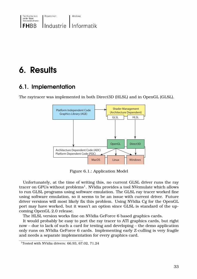
The raytracer was implemented in both Direct3D (HLSL) and in OpenGL (GLSL).

Shader Management(Architecture Dependent)

Platform Independent CodeGraphics Library (AGE)

GLSL

Architecture Dependent Code (ADC)Platform Dependent Code (PDC)

OpenGL Direct3D

Linux WindowsMacOS

HLSL

Figure 6.1.: Application Model

Unfortunately, at the time of writing this, no current GLSL driver runs the raytracer on GPUs without problems1. NVidia provides a tool NVemulate which allowsto run GLSL programs using software emulation. The GLSL ray tracer worked fineusing software emulation, so it seems to be an issue with current driver. Futuredriver versions will most likely fix this problem. Using NVidia Cg for the OpenGLport may have worked, but it wasn’t an option since GLSL is standard of the up-coming OpenGL 2.0 release.

The HLSL version works fine on NVidia GeForce 6 based graphics cards.It would probably be easy to port the ray tracer to ATI graphics cards, but right

now – due to lack of such a card for testing and developing – the demo applicationonly runs on NVidia GeForce 6 cards. Implementing early Z-culling is very fragileand needs a separate implementation for every graphics card.

1Tested with NVidia drivers: 66.93, 67.02, 71.24

33

There are only little optimizations in the current HLSL/GLSL code, there is roomfor much improvement. For this first implementation, clarity was the most impor-tant factor.

Figure 6.2.: Screenshot of the Demo Application

6.2. Benchmark

Rendering a scene can be done on both CPU and GPU. Both implementations usethe same approach (uniform grid, non recursive ray tracing), which allows bench-marking, however both versions have potential for optimizations.

6.2.1. Demo Scenes

There are 3 scenes. Scene A only has a few polygons, B has low polygon objectsdistributed in the scene and C has high and low polygon objects distributed in thescene.

34

Scene Description TrianglesA 3 Boxes 36B Cubes distributed in room 2064C High and low polygon objects 61562

Table 6.1.: Demo Scenes A,B, and C

Figure 6.3.: Scene A

Figure 6.4.: Scene B

35

Figure 6.5.: Scene C

Figure 6.6.: Scene B - Ray Traced

Figure 6.7.: Scene C - Ray Traced

36

6.2.2. Result: GPU

0.00

1.00

2.00

3.00

4.00

5.00

Ren

der

Tim

e [s

]

Scene AScene BScene C

Scene A 0.25 0.13 0.08

Scene B 0.51 0.26 0.17

Scene C 4.04 2.03 1.36

6600 PCI Express 6800 GT 6800 Ultra

Figure 6.8.: Render Time for Different GPUs, Grid Size: 20x20x20

0.00

0.02

0.04

0.06

0.08

0.10

0.12

Scene A 0.06 0.05 0.08 0.11

2x2x2 10x10x10 20x20x20 30x30x300.00

0.20

0.40

0.60

0.80

1.00

1.20

1.40

Scene B 1.32 0.22 0.17 0.32

2x2x2 10x10x10 20x20x20 30x30x300.00

5.00

10.00

15.00

20.00

25.00

30.00

35.00

40.00

Scene C 36.2 4.03 1.36 1.32

2x2x2 10x10x10 20x20x20 30x30x30

Figure 6.9.: Render Time: Different Grid Size, GeForce 6800 Ultra

All images were rendered into a 256x256 image/texture.

37

6.2.3. Result: GPU vs. CPU

0.00

0.20

0.40

0.60

0.80

1.00

1.20

1.40

1.60

1.80

2.00

Render Time [s]

Scene A

Scene B

Scene C

Scene A 0.08 0.24 0.15 0.08

Scene B 0.17 0.34 0.27 0.14

Scene C 1.36 1.72 1.03 0.81

NV40 [400 MHz]Pentium 4 [2.0

GHz]

Pentium 4 [3.0

GHz]AMD 64 [2.2 GHz]

Figure 6.10.: GPU vs. CPU: 1 Iteration

0.00

1.00

2.00

3.00

4.00

5.00

6.00

7.00

8.00

Ren

der T

ime

[s]

2 Iterations 0.32 0.15 0.56 0.34 3.24 2.79

3 Iterations 0.4 0.24 0.68 0.51 4.58 4.24

5 Iterations 0.57 0.42 0.88 0.85 6.93 7.14

Scene A:

CPU

Scene A:

GPU

Scene B:

CPU

Scene B:

GPU

Scene C:

CPU

Scene C:

GPU

Figure 6.11.: CPU vs. GPU: Different Iterations: Pentium 4 [2.0 GHz] vs. NVidiaGeForce 6800 Ultra

38

All images were rendered into a 256x256 image/texture.

6.3. Observations

A higher number iterations usually lead to a high amount of additional early-zculling passes and usually at a iteration depth of 4+ only few rays are still active.Using a high number of z-culling passes for only a few rays is very inefficent.

6.4. Possible Future Improvements

• Support for Textures, both procedural and bitmap based.

• Add transparent materials and use refraction.

• Implement GPU based Path Tracing.

• The application could be extended to support ray traced shadows in real timerendering2.

• Animated objects - with limited polygons - could be added to the static sceneusing a bounding box hierarchy.

2Regular triangle based real time rendering which is currenty used in computer games is meanthere.

39

7. Conclusion

Experiments with a lot of different scenes showed that ray tracing on GPU is feasi-ble.

Although there is enough computing power in a GPU, Ray Tracing is not yet muchfaster than an equal CPU implementation. There is also a possible instability withcertain hardware configurations. On Pentium based machines there are no errorswhen ray tracing with GPU, while on a AMD64 system there were artifacts whenrendering bigger scenes.

If GPU hardware would allow multipassing as presented in 4.1 directly on hard-ware - without the need of a CPU / occlusion query based control - a major gain inperformance would be possible.

GPUs don’t have much RAM and there are hardware specific limitations whenrendering high resolution meshes with a lot of textured objects.

However, if the current trend of enhancing graphics cards continues the sameway like past years, future generations of GPUs will make real time ray tracing incomputer games possible, provided that stability of graphics card drivers will bebetter.

40

A. Screenshots

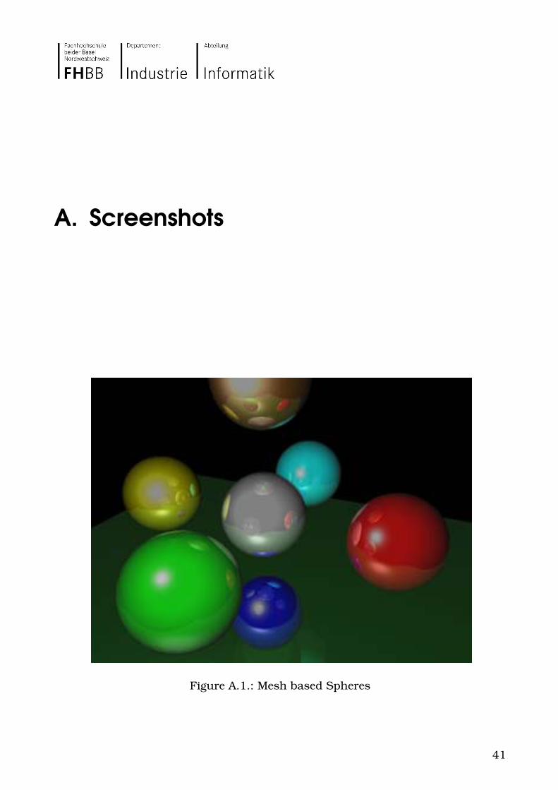
Figure A.1.: Mesh based Spheres

41

Figure A.2.: Reflect Box

Figure A.3.: Teapot (60k Triangles)

42

Bibliography

[1] John Amanatides, Andrew Woo. A Fast Voxel Traversal Algorithm for Ray Trac-ing, 1987.

[2] J. Avro, and D. Kirk. A survey of ray tracing acceleration techniques. In AnIntroduction to Ray Tracing, A. Glassner, Ed., pages 201–262. Academic Press,San Diego, CA, 1989.

[3] J. F. Blinn. Simulation of Wrinkled Surfaces, In Proceedings SIGGRAPH 78,pp. 286-292, 1978.

[4] I. Buck. Brook: A Streaming Programming Language, October 2001.

[5] Robert L. Cook, Kenneth E. Torrance. A reflectance model for computer graph-ics, 1981.

[6] Randima Fernando, Mark J. Kilgard. The Cg Tutorial, April 2003.

[7] GPGPU http://www.gpgpu.org, 2004.

[8] Michael McCool. http://libsh.sourceforge.net/, 2004.

[9] NVidia Corporation, NVIDIA GPU Programming Guide Version 2.2.0, 2004

[10] John D. Owens. GPUs tapped for general computing, EE Times, December2004

[11] Timothy John Purcell, Ray Tracing on a Stream Processor, 2004.

[12] Timothy J. Purcell, Ian Buck, William R. Mark, Pat Hanrahan. Ray Tracing onProgrammable Graphics Hardware, 2002

[13] Randi J. Rost. OpenGL Shading Language, February 2004

[14] Jorg Schmittler, Daniel Pohl, Tim Dahmen, Christian Vogelgesang, and PhilippSlusallek. Realtime Ray Tracing for Current and Future Games, 2004

43

[15] Ingo Wald. Realtime Ray Tracing and Interactive Global Illumination, January2004.

[16] Turner Whitted. An Improved Illumination Model for Shaded Display, June1980.

44