Rationality and Coherent Theoriesof Strategic Behavior†

Faruk Gul

Northwestern University

November 1999

† This paper relies heavily on the work of Douglas Bernheim, David Pearce and Phil Reny. I have alsobenefited from discussions with Dilip Abreu, Douglas Bernheim, Ken Binmore, Eddie Dekel-Tabak, DavidKreps, David Pearce, Andrew Postlewaite, Phil Reny, Hugo Sonnenschein and Robert Wilson on Nashequilibrium and subgame perfection. Geir Asheim, Chris Avery, Outi Lantto and Sonia Weyers have alsoprovided many valuable comments and criticisms. Financial support from the Alfred P. Sloan Foundationand the National Science Foundation is gratefully acknowledged.

Running head: Rationality and Coherent Theories

Faruk GulDepartment of EconomicsNorthwestern UniversityEvanston, IL 60208-2600

Abstract

A non-equilibrium model of rational strategic behavior that can be viewed as a refine-ment of (normal form) rationalizability is developed for both normal form and extensiveform games. This solution concept is called a τ -theory and is used to analyze the mainconcerns of the Nash equilibrium refinements literature such as dominance, iterative dom-inance, extensive form rationality, invariance, and backward induction. The relationshipbetween τ -theories and dynamic learning is investigated.

JEL classification number C72

1. Introduction

In their work on rationalizability, Bernheim [5] and Pearce [19] have shown that Nash

equilibrium behavior can not be deduced solely from assumptions regarding the rationality

of players and their knowledge of the rationality of their opponents. In particular, they have

shown that all rationalizable strategies, and only rationalizable strategies, are consistent

with the assumption that rationality is common knowledge.

Identification of the implications of the common knowledge of rationality is undoubt-

edly a most significant contribution to the theory of strategic behavior. Nevertheless, both

Bernheim and Pearce have noted that game theory need not restrict itself to this task

and that other factors may well be incorporated into the analysis. Specifically, Bernheim

has analyzed how learning and dynamics could impose restrictions on the beliefs of ratio-

nal players about the behavior of other rational players, while Pearce has considered the

implications of the extensive form. Both have dealt with the possible impact of rational

players’ concerns regarding “error” or irrationality on the part of their opponents. Similar

ideas have been advanced within the context of Nash equilibrium refinements as criteria

for ruling out certain Nash equilibria.1

The purpose of this paper is to develop a solution concept or a class of solution

concepts that describes how factors that can not be deduced from rationality assumptions

might interact with the Rationality Hypothesis to yield predictions about behavior which

are more restrictive than rationalizability.2 That is, I wish to present a general framework

for studying and/or developing non-equilibrium refinements of rationalizability.

All of the subsequent analysis will be guided by the following principles:

(1) I wish to distinguish between what is being assumed (i.e., exogenous) and what is

being deduced (i.e., endogenous). In particular, I will take the beliefs of rational players

regarding the behavior of their opponents as exogenous and the predictions regarding

the behavior of rational agents to be endogenous. I will insist that all conclusions

regarding the endogenous variable are implied by (rather than being merely consistent

with) the exogenous variables and the Rationality Hypothesis.

1 Selten [28] makes explicit reference to mistakes and irrationality.2 The Rationality Hypothesis is the assertion that rationality (i.e., expected utility maximization given

subjective probability assesment about opponents’ behavior) is (almost) common knowledge.

1

The difficulty in maintaining that a particular strategy must be played, even though a

continuum of other strategies would yield the same payoff given the conjecture held by

the player, is acknowledged within the Nash equilibrium framework as well (see Harsanyi

[12]). The first principle above reflects the same concern.

(2) I will insist that the assumptions regarding beliefs should be justifiable by the resulting

model. That is, the set of allowable beliefs of player i should include the convex hull

of the set of allowable profiles of strategies of player i’s rational opponents.

G 1

x

a

b

4, 1

0, 0

0, 0

1, 4

y

5, 0c –5,1

Figure 1.

Both of these principles can easily be illustrated with the aid of the game G1 in

figure 1. Let Ci for i = 1, 2 be the set of conjectures and Ri be the set of predictions

for player i. Consider the case in which C1 ={

15x + 4

5y}

and C2 ={

45a + 1

5b}. First

let R1 = C2 and R2 = C1. Note that a model with (Ci)ni=1 as the (exogenous) beliefs

and (Ri)ni=1 as the predicted behaviors is ruled out by principle (1) above since with these

restrictions on beliefs the Rationality Hypothesis does not enable us to deduce that any

other strategy with support {a, b} will not be played. Hence, principle (1) rules out the

possibility of interpreting any non-degenerate mixed strategy as a singleton prediction of

behavior.

Next, let R1 ={αa + (1 − α)b | α ∈ [0, 1]

}and R2 =

{βx + (1 − β)y | β ∈ [0, 1]

}.

Note that the model (R1, R2, C1, C2) satisfies the requirements of principle (1) but fails

to satisfy principle (2). Thus, principle (2) rules out the possibility of interpreting any

mixed strategy equilibrium as an equilibrium in beliefs. Principle (2) reflects the view

that it is unreasonable to insist that player 1 must believe 15x + 4

5y given the inability

2

of the theory to exclude any strategy in R2 as a possible rational choice for player 2.

The need to relate the predicted behavior to the initial restrictions on beliefs is shared by

the current and nearly all (Nash equilibrium and non-equilibrium) approaches to rational

strategic behavior. The novelty here is in the nature of this relation. The requirement

in principle (1), that conclusions regarding behavior should be implied by the exogenous

restrictions and the Rationality Hypothesis, together with the requirement in principle (2),

that the set of allowable beliefs about rational opponents should include the convex hull

of the allowable action profiles, will be called coherence .

(3) I will distinguish between rational and irrational players. It is not asserted that all

players are rational. However, the conclusions of the theory are only about the be-

havior of rational players and the coherence principle is imposed only on rational

players’ beliefs about rational opponents. Irrationality plays a role only because ra-

tional players assign some probability to the irrationality of their opponents. Hence,

the only beliefs that are considered are the beliefs of the rational players. I will focus

on the case in which it is common knowledge that players assign high probability to

the rationality of their opponents.

(4) In extensive form games, I will take the position that the Rationality Hypothesis offers

no guidance to a player who is in a position to choose an action after his rationally

held conjecture is violated.

This final principle is motivated by the work of Basu [2], Reny [23] and others and by what

was previously known as the paradox of backward induction.

In sections 2 and 3, I will formally define the notion of a τ -theory (for normal and

extensive form games) which results from the four principles above. Every τ -theory is

a refinement of rationalizability and shares many of the properties of the collection of

rationalizable strategies. The notion of a τ -theory enables a classification of the kind of

restrictions that have been employed in the refinements literature. Specifically, I will argue

that iterated dominance (Proposition 5) and backward induction (Proposition 8) can be

viewed, for two-person games, as restrictions on the nature of irrational behavior. I will

show in Proposition 7 that if (trembling-hand) perfection is imposed, then rationality in

3

the extensive form is equivalent to rationality in the equivalent normal form (invariance);

otherwise it is not. I will conclude that many of the apparent paradoxes in game theory

arise from game theorists’ insistence on interpreting possibly plausible restrictions on the

nature of irrational behavior (e.g., assessments of the relative likelihoods of various kinds

of errors) as implications of rationality. In section 4, I will analyze the possibility that

naive learning might substitute for the Rationality Hypothesis.

The works of Bernheim [5], Pearce [19], and Reny [23] play a central role in the

analysis below. Other related work on axiomatic foundations for perfection by Borgers

[8] and Dekel and Fudenberg [10], or iterated dominance by Borgers and Samuelson [9]

and Samuelson [26], will also be discussed. The section on learning relates to the work of

Milgrom and Roberts [17] and Sanchirico [27]. Rabin [20] also explores the possibility of

incorporating exogenous restrictions into the analysis of rational strategic behavior. His

consistent behavioral theories (CBT’s) have features in common with τ -theories for two-

person games. However, CBT’s may fail the coherence criterion by violating principle (1)

above. The section on normal form games relates to Rabin’s work. Within the refinements

literature, comments similar in spirit to my analysis of normal form games appear in Kalai

and Samet [13] and ideas related to my view of extensive form games can be found in

Reny [22]. However, the fact that the last two papers have taken Nash equilibrium as their

starting point makes any detailed comparison impossible.

2. Normal Form Games

In this section, I will utilize the principles outlined in the introduction to motivate

the definition of a normal form τ -theory. I will argue that the first three principles of the

introduction lead to the notion of a τ -theory. I will then discuss the relationship between

τ -theories and rationalizability, perfection, and iterative (weak) dominance. Before under-

taking the formal analysis, some basic definitions and a brief review of rationalizability are

in order.

Let G = (Ai, ui)ni=1 denote a finite n-person game. Hence, for i = 1, 2, . . . , n, Ai

is a finite set and ui : A → IR is a (von Neumann-Morgenstern) utility function, where

A =∏n

i=1 Ai. I assume that players have preferences over Si×S−i where A−i =∏

j 6=i Aj ,

4

Si and S−i denote the set of all probability distributions on Ai and A−i, respectively,

and the actions ai ∈ Ai and a−i ∈ A−i are identified with the appropriate degener-

ate distributions. For s−i ∈ S−i, let πj(s−i) ∈ Sj for j 6= i denote the marginal dis-

tribution of s−i on Aj . Finally let Ui : Si × S−i → IR be defined by Ui(si, s−i) =∑

ai

∑a−i

ui(ai, a−i)si(ai)s−i(a−i). I will refer to Si as the set of all mixed strategies and

S−i as the set of all conjectures of player i. For any set X ⊂ Si, Xi denotes the convex

hull of Xi and IntXi ={si ∈ Xi | s′i ∈ X , s′i(ai) > 0 implies si(ai) > 0

}.

The mapping Bi : S−i → Si denotes the best response correspondence of i. Hence,

si ∈ Bi(s−i) iff Ui(si, s−i) ≥ Ui(s′i, s−i) for all s′i ∈ Si. (Correlated) Rationalizability will

play an important role throughout this paper. A formal definition is presented below.

Definition 1: For all i = 1, 2, . . . , n, let Ri(0) = Si and Ri(t + 1) = {si ∈ Si | si ∈

Bi(s−i) for some s−i ∈ S−i such that πj(s−i) ∈ Rj(t) for all j 6= i}. The set R∗i =⋂∞

t=0 Ri(t) is called the set of rationalizable strategies of player i. Let ρ∗ := (R∗i )ni=1.

It is easy to verify that Ri(t + 1) ⊂ Ri(t) for all i and there exists some t such that for all

t ≥ t and i = 1, 2, . . . , n, Ri(t) = R∗i (see Pearce [19]).

The iterative procedure used above to define rationalizability can be interpreted as

follows:3

Suppose every player choosing a strategy behaves according to the following

axioms of rationality which I will call the “Rationality Hypothesis.”

(R1): Every player i has some conjecture s−i regarding the behavior of his oppo-

nents. Player i chooses some strategy si which maximizes his payoff given

his conjecture s−i.

(R2): Every player i knows (R1) above and knows that every player j 6= i knows

(R1) above and knows that every player j 6= i knows that every player k 6= j

knows (R1) above, etc.; that is, (R1) is common knowledge.4

3 Note that the definition above, and all of the subsequent analysis, allows for correlated conjectures,while Bernheim’s and Pearce’s original formulation does not. For an argument as to why correlatedconjectures may be appropriate, see Aumann [1]. The current formulation not only allows correlation, butmakes it impossible to restrict the extent of correlation. Some implications of this are discussed below.

4 It is possible, and in fact appropriate, to replace the phrase “common knowledge” with “commonbelief” throughout this paper. However, I will for the sake of simplicity reserve the word “belief” forconjectures about behavior, i.e., the elements of the set S−i.

5

It is easy to see that (R1) implies that every player i will choose some strategy si ∈

Ri(1), since Ri(1) is the set of all strategies which best respond to some conjecture s−i.

But by (R2), every player knows this. Hence by (R1), every player i will choose a best

response to some conjecture s−i such that s−i assigns zero probability to any strategy not

in Rj(1) for all j 6= i. But this is equivalent to saying that every player i will choose a

strategy in Ri(2). Repeating the above argument yields that every player i will choose a

strategy such that si ∈ R∗i =⋂

t≥1 Ri(t). Thus, (R1) and (R2) imply that every player will

choose some rationalizable strategy. A similar argument establishes that, in fact, every

si ∈ R∗i is a choice consistent with (R1) and (R2). Thus, the conclusion that every player

will choose a rationalizable strategy is equivalent to the assertion that every player will

choose a strategy as if (R1) and (R2) are satisfied.

As I have stated in the introduction, much of the criticism of rationalizability centers

on the fact that it rules out only those strategies that are inconsistent with (R1) and (R2).

Consider again the game G1 from figure 1 in section 1 above. Suppose in some context,

in addition to (R1) and (R2), it became common knowledge that player 2 believes that

player 1 will not play a. Then by (R1), player 2 will play y. But then (R2) implies that

player 1 knows that player 2 will play y. Hence (R1) implies that player 1 will play b.

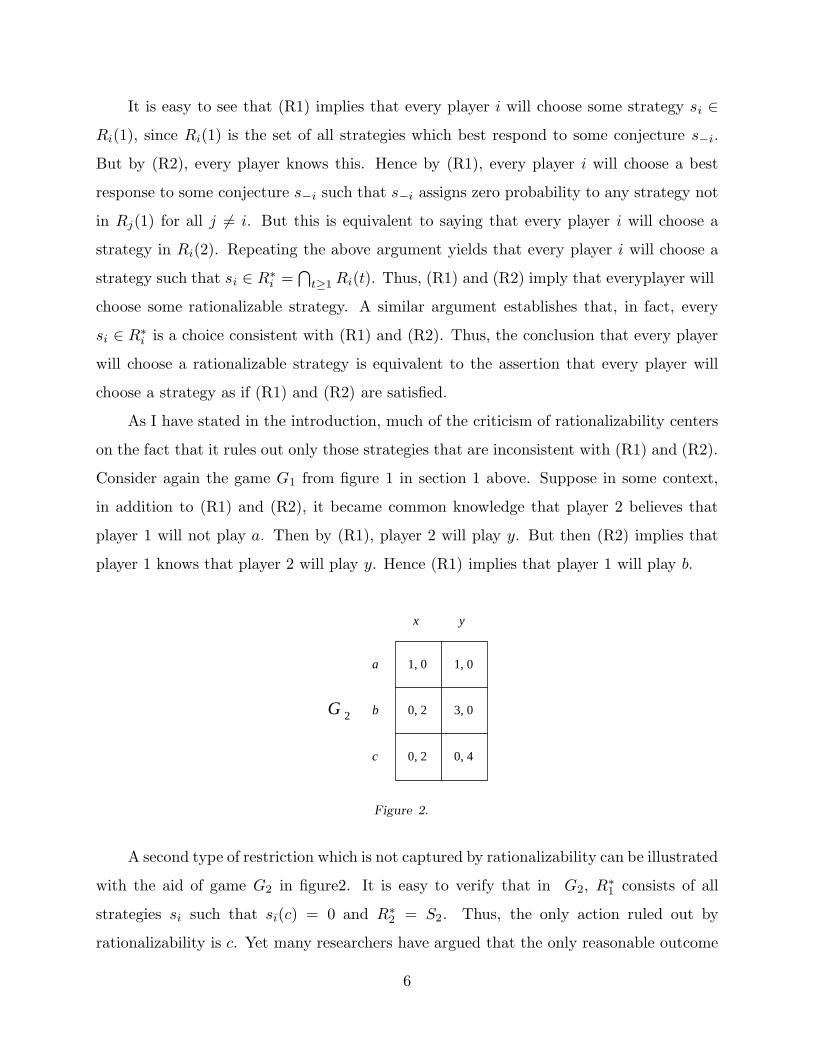
x y

G 2

a

b

c

1, 0

0, 2

0, 2

1, 0

3, 0

0, 4

Figure 2.

A second type of restriction which is not captured by rationalizability can be illustrated

with the aid of game G2 in figure 2. It is easy to verify that in G2, R∗1 consists of all

strategies si such that si(c) = 0 and R∗2 = S2. Thus, the only action ruled out by

rationalizability is c. Yet many researchers have argued that the only reasonable outcome

6

of this game is (1, 0). Indeed (1, 0) is the only payoff pair which is consistent with Nash

equilibrium or Pearce’s [19] cautious rationalizability. A possible argument for insisting on

(1, 0) as the only reasonable outcome of this game is the following:

Suppose we require that both players assign some small probability to the

possibility that their opponents might make an error—that is, they might be

irrational. Suppose we also assert that irrational players are capable of choosing

any strategy. Finally, we assume that even if player 1 is irrational, he is much less

likely to play c than a or b (after all, c is strictly dominated). This would imply

player 2, if rational, should not play y (since c is much less likely than b). But

knowing this and also assigning a high probability to the rationality of player 2,

player 1 should play a. Thus we are left with the unique strategy pair (a, x).

The solution concept to be defined in this section will allow for both types of re-

strictions described with the aid of G1 and G2 above. The basic idea is to modify the

two axioms (R1) and (R2) so as to incorporate exogenous restrictions on beliefs. Thus,

consider the following modified Rationality Hypothesis:

(T1): Every player i, if rational, has some conjecture s−i regarding the behavior

of his opponents. According to this conjecture, player j 6= i, if rational,

will choose some strategy in a set R0j ; if irrational, in a set Σj . Moreover,

there is probability at least 1 − ε(where ε ∈ (0, 1)

)that each opponent is

rational and some positive probability each opponent is irrational. Finally,

if rational, player i chooses a strategy si which maximizes his payoff given

his conjecture s−i.

(T2): Every player i, if rational, knows (T1), knows that every player j 6= i, if

rational, knows (T1), knows that every rational player j 6= i knows that

every rational player k 6= j knows (T1), etc. That is, (T1) is common

knowledge among rational players.

The real numbers ε and τ0 ≡ (R0i , Σi)

ni=1 for all i are to be viewed as parameters of

the given strategic situation. Given these initial parameters, (T1) and (T2) will enable

players to make further deductions regarding the behavior of rational players. The analysis

7

of this process will yield an iterative procedure similar to the one implied by (R1) and

(R2) above. Specifically, (T1) states that every rational player will best respond to some

allowable conjecture, where an allowable conjecture places at least a 1 − ε probability to

the rationality of his opponents and some probability to the irrationality of his opponents.

Moreover, each player i knows that a rational opponent j chooses a strategy in R0j and an

irrational opponent j chooses a strategy in Σj . Let R1i denote the set of all best responses

to such conjectures. But now, by (T2), each player i can refine his understanding of what

a rational player will do and conclude that opponent j, if rational, will choose a strategy

in R1i ∩ R0

i . But by (T1), this reduces the set of conjectures that a rational player may

entertain, and hence further reduces the set of possible strategies that rational players can

choose and so on. Definitions 2 and 3 below provide some notation regarding this iterative

process.

Definition 2:

(a) Let Pi = 2Si , Υi = Pi × Pi, P =

∏ni=1Pi, and Υ =

∏ni=1 Υi.5

(b) Let º be the following binary relation on P: (Ri)ni=1 º (R′i)

ni=1 iff Ri ⊇ R′i for all i.

Definition 3:

(a) For any τ = (ρ, ρ′) =((Ri)

ni=1, (Σi)

ni=1

)and ε > 0, define Cε

−i(τ) :={s−i ∈ S−i | for

all j 6= i, πj(s−i) = αjs1j + (1− αj)s

2j for some αj ∈ [ 1− ε, 1), s1

j ∈ Rj and s2j ∈ Σj

}.

Let C−i(τ) ≡ C−i(ρ) ={s−i ∈ S−i | for all j 6= i, πj(s−i) ∈ Rj

}.

(b) For any τ = (Ri,Σi)ni=1 and ε > 0, define Bε

i(τ) ={si ∈ Bi(s−i) | s−i ∈ Cε

−i(τ )}. By

convention, Bεi(τ) = ∅ if Rj = ∅ for some j 6= i and Bε(τ) = (Bε

i(τ ))ni=1.

For τ = (ρ, ρ′) we will call C−i(τ ) the set of all τ -allowable, or equivalently ρ-allowable,

conjectures and Cε−i(τ) the set of all (ε − τ)-allowable conjectures. The mapping Bε

describes the rational response to a given set of parameters.

Letting ε > 0 and τ0 = (ρ0, ρ′), define τk+1 =((

Bi(τk) ∩ Rk

i

)n

i=1, ρ

)where ρk =

(Rki )n

i=1 and τk = (ρk, ρ′) for all k. Let Ri =⋂

k≥1 Rki and ρ = (Ri)

ni=1. As I have argued

above, the implication of (T1), (T2), and the initial parameters ε and τ0 is that every

rational agent i must choose a strategy in Ri. Given ε and τ0, the following problems

5 I will write both τ = (Ri, Σi)ni=1 and τ = ((Ri)n

i=1, (Σi)ni=1) to denote a generic element τ of Υ.

8

could arise. It could be that some Rki = 0 for some k (and hence, by our convention in

defining Bεi , Rj = 0 for all j = 1, . . . , n). In this case, we conclude that the exogenous

restrictions (i.e., parameters) (T1) and (T2) are logically inconsistent. Or it could be

that ρ 6= Bε(ρ, ρ′). Specifically, it could be that ρ 6= Bε(ρ, ρ′) and Bε(ρ, ρ′) º ρ. In

this case, we conclude that ε and τ are not coherent parameter values as discussed in the

introduction: ρ entails restrictions on behavior that can not be justified by (T1) and (T2)

and the initial restrictions on beliefs. To see an example of this, reconsider the example

of incoherence discussed in the introduction: Let ρ0 = ρ′ denote the behavior associated

with the mixed strategy equilibrium of G1 in figure 1. Then ρ = ρk = ρ0 for all k. But

Bε1(ρ

0, ρ0) =({

αa + (1−α)b | α ∈ [0, 1]}, S2

)6= ρ0 and hence ε > 0 and τ 0 = (ρ0, ρ0) are

not coherent values of these parameters.

Proposition 0 below establishes certain basic properties of the map Bε and the ρk’s

defined above. All proofs are in the appendix.

Proposition 0:

(i) ε ≥ ε′, ρ º ρ′, and ρ º ρ′ implies Bε(ρ, ρ) º Bε′(ρ′, ρ′).

(ii) Let ε ∈ (0, 1) and ρ′ ∈ P. Fix ρ0 = (R0i )

ni=1 ∈ P . Define ρk = (Rk

i )ni=1 for k = 1, 2, . . .

as follows: Rk+1i = Bi(ρ

k, ρ′) ∩ Rki . Then there exists k∗ such that ρk = ρk∗ for all

k ≥ k∗. Moreover, ρ0 º ρ and ρ = Bε(ρ, ρ′) implies ρk∗ º ρ.

(iii) For all τ = (ρ, ρ′) ∈ Υ, there exists ε ∈ (0, 1) such that for all ε ∈ (0, ε), Bε(τ) = Bε(τ).

Moreover, for ρ = (Ri)ni=1, Ri is closed for every i implies ε can be chosen so that

Bε(τ) ⊂ Bε(ρ, ρ) = Bε(ρ, ρ) for all ε ∈ (0, ε).

Part (iii) of Proposition 0 states that the algorithm implied by T1 and T2 ends in a

finite number of steps. The resulting prediction of behavior is the unique maximal (for the

binary relation º) fixed point of the mapping Bε : Υτ0 → Υτ0 , where Υτ0 ={(ρ, ρ′) | ρ º

ρ0}.

The focus of this paper is on the case where ε is arbitrarily small. However, we wish to

be somewhat literal about the existence of possible irrationality. Part (iii) of Proposition 0

shows that these two desires are not inconsistent: all Bε’s are identical for ε sufficiently

small.

9

Definition 4: Let Bi(τ ) =⋂

ε>0 Bεi(τ) and B(τ ) = (Bi(τ))n

i=1. Then τ = (ρ, ρ′) ∈ Υ is

a τ -theory iff B(τ ) = ρ.

Observe that parts (i) and (iii) of Proposition 0 establish that, for any τ = (Ri, Σi)ni=1

such that Ri 6= ∅ 6= Σi for all i, Bi(τ) is non-empty. Also note that in Definition 4,

restrictions on the beliefs of rational players regarding the behavior of irrational players

are made explicit, but restrictions on the beliefs of rational players regarding the behavior of

other rational players are suppressed. This creates no problem. The algorithm described in

analyzing (T1) and (T2) (i.e., ρk for k = 1, 2, . . . , k∗ as defined in part (ii) of Proposition 0)

suggests the following alternative definition: ρ is τ -rational behavior iff there exists τ0 =

(ρ0, ρ′) ∈ Υ such that ρk = (Rki )n

i=1, Rk+1i = Bi(ρ

k, ρ′) ∩ Rki for k = 1, 2, . . . , k∗, and

ρ = ρk∗ =(⋂

k≥1 Rki

)n

i=1. Thus, any behavior ρ is τ -rational iff there exist some parameters

ε and τ 0 such that (T1) and (T2) enable us to conclude that all rational players will

behave according to ρ. But if such a τ0 exists, and coherence is satisfied, we have Ri =

Bi(τk∗) ∩ Rk∗

i = Bi(τk∗) so that the same ρ could be reached if we started from (ρ, ρ′)

rather than τ 0 = (ρ0, ρ′), which is the motivation behind Definition 4.

The following classification of exogenous restrictions will be useful in understanding

many of the ideas of the refinement literature.

Definition 5: A τ -theory τ = (ρ, ρ′) imposes no type 1 restrictions (i.e., exogenous

restrictions on the beliefs of rational players about the behavior of other rational opponents)

iff τ = (ρ, ρ′) is a τ -theory implies ρ º ρ.

Definition 5 states that, given (Σi)ni=1, if imposing no exogenous restrictions on beliefs

about rational players’ behavior does not lead to a τ -theory with ρ as the predicted rational

behavior, then the τ -theory is said to impose type 1 restrictions.

Definition 6: A τ -theory τ = (ρ, ρ′) imposes no type 2 restrictions (i.e., exogenous

restrictions on the behavior of irrational players) iff(ρ, (Si)

ni=1

)is a τ -theory.6

The work of Rabin [20] introduces a concept similar to the notion of a τ -theory.

Rabin’s consistent behavioral theories allow for (exogenous) restrictions on predicted be-

havior, but rule out type 2 restrictions. One of his motivations for allowing restrictions on

6 It follows from Lemma 0 of the Appendix and Proposition 0 above that τ is a τ -theory with no type 2restrictions iff B(τ ) is an exact set in the sense of Basu and Weibull [3].

10

predictions is to identify candidates for what may be the best (subjective) assessment of

an outside observer. Hence it is not required that all conclusions regarding behavior are

deduced from restrictions on beliefs in Rabin’s notion of a consistent behavioral theory. In

the current framework, predictions consist of the (common knowledge) implications of the

assumed restrictions on beliefs and the Rationality Hypothesis. They do not incorporate

subjective assessments of any outside observer. Rabin’s [20] and [21 work and the related

work of Farrell [11] on cheap talk share with this paper the objective of identifying exoge-

nous restrictions on rational behavior/beliefs. Rabin [20] focuses on psychological/cultural

factors as encapsulated by the idea of a focal point, while Rabin [21] and the work of

Farrell [11] deal mostly with communication as the source of these restrictions.

The remainder of this section will be concerned with establishing the relationship

between τ -theories (and their exogenous restrictions) and various basic game theoretic ideas

such as rationalizability, (trembling-hand) perfection, and iterative (weak) dominance.

Definition 7: A τ -theory τ =(ρ, (Σi)

ni=1

)is a perfect τ -theory iff Σi ⊂ IntSi for all

i. That is, in a perfect τ -theory, rational players are required to assign some positive

probability to every action.

Note that if a τ -theory is of the form τ = (ρ, ρ), then irrational players are expected

to behave just like the rational players. Thus, rationality is common knowledge in such

a τ -theory. Proposition 1 below establishes that assuming the chance of irrationality is

sufficiently small (which is implicit in the notion of a τ -theory) and imposing no type 2

restrictions is equivalent to assuming that rationality is common knowledge. That is, if

rational players know nothing (or agree on nothing) regarding the nature of irrational

behavior other than that it is unlikely, then the resulting behavior is as if rationality is

common knowledge.

Proposition 1: For any game G, (ρ, ρ) is a τ -theory iff(ρ, (Si)

ni=1

)is a τ -theory.

Proposition 2 below establishes the strong connection between the notion of a τ -theory

and rationalizability. It shows that rationalizability is a (common knowledge) τ -theory and

that every τ -theory is a refinement of rationalizability.

11

Proposition 2: For any game G, τ∗ = (ρ∗, ρ∗) is a τ -theory. Moreover, τ = (ρ, ρ′) is a

τ -theory implies ρ∗ º ρ.

One of the more puzzling problems of strategic analysis is the relationship between

rationality and (weak) dominance. As noted by Pearce [18] and Samuelson [26], if the

sole reason for strategy a’s dominance over b is that a does better against some irrational

strategy of the opponent, then insisting that (weakly) dominated strategies are never played

conflicts with the hypothesis that rationality is common knowledge.

Dekel and Fudenberg [10] have explored the possibility that dominance might be

explained by (a small amount of) uncertainty about the payoff of the opponent. They

show that this leads to what I will call perfect τ -rationalizability. Proposition 3 below

establishes that perfect τ -rationalizability is a perfect τ -theory. Recently, Borgers [8] has

independently attempted to provide decision theoretic foundations for perfection (or cau-

tiousness). He shows that the assumption of approximate common knowledge of rationality

leads also to perfect τ -rationalizability. While there are some differences in the approaches

of Dekel and Fudenberg [10], Borgers [8], and the current paper, it is noteworthy that

each ultimately identifies perfect τ -rationalizability.7 Apparently, being explicit about the

source of cautiousness either as uncertainty about an opponent’s payoffs or his rationality,

in the absence of other restrictions, leads to perfect τ -rationalizability. Proposition 4 below

establishes that perfect τ -rationalizability is the weakest perfect τ -theory.

Definition 8: For any game G, let Rui denote the set of undominated strategies for

player i. That is, si ∈ Rui if and only if, for all si ∈ Si, either Ui(si, s−i) = Ui(si, s−i) for

all s−i ∈ S−i or there exists s−i such that Ui(si, s−i) > Ui(si, s−i). Let Aui denote the

set of pure undominated strategies, i.e., Aui = Ai ∩Ru

i . Let Gu denote the game obtained

from G by removing all dominated pure strategies, i.e., Gu ={(Au

i , ui)ni=1

}. The set of

perfectly τ -rationalizable strategies Rpi is defined as Rp

i = R∗i (Gu)∩Rui ; that is, Rp

i is the

intersection of the rationalizable strategies of Gu with the undominated strategies of G.

Let ρp := (Rpi )n

i=1.

7 Perfect τ-rationalizability entails removing all weakly dominated strategies in the first round andremoving only strictly dominated strategies in the subsequent rounds; while iterative dominance entailsremoving all weakly dominated strategies in every round. Obviously, the former is a more stringentrequirement than admissibility (i.e., weak dominance), but less stringent than iterative dominance.

12

Note that the reason for defining Rpi as the intersection of R∗i (G

u) and Rui instead of

just taking R∗i (Gu) is that R∗i (G

u) may contain mixed strategies that are dominated in

the game G.

It follows from elementary arguments that perfect τ -rationalizable strategies exist for

every game G. Borgers [8] has shown that what I have called perfect τ -rationalizability is

different from perfect rationalizability in the sense of Bernheim [5].8

Proposition 3: For any game G, τp =(ρp, (Int Si)

ni=1

)is a perfect τ -theory.

Proposition 4: For any game G, τ = (ρ, ρ′) is a perfect τ -theory implies ρp º ρ.

As I have stated in the introduction, the position I take in this paper is that while

it may be useful to explicitly state the relationship between the nature of the exogenous

restrictions and the implied behavior, deciding which kind of restrictions are appropriate

in any given context is often not a matter of a priori analysis. This is particularly true of

type 2 restrictions since these involve the behavior of irrational players. Moreover, both for

type 1 and type 2 restrictions, it is very difficult to argue that the normal (or even extensive)

form contains adequate or even particularly useful information about the relative merits

of various restrictions. Presumably, one of the main motivations of studying a variety of

strategic problems within the sparse formalism of normal and extensive games is the desire

to concentrate entirely on the strategic aspects and to ignore the institutional complexity,

the details of the presentation, the underlying social norms, etc. In most applications,

the minor effects that can be attributed to factors such as symmetry of payoffs and the

labeling of strategies are sure to be overwhelmed by the kind of factors and information

that was suppressed in obtaining an abstract normal form for representation. For a social

psychologist or sociologist, normal and extensive form games should constitute very barren

territory.

The final task of this section is to identify the relationship between iterative dominance

and τ -theories. Since the removal of dominated strategies is taken to be a basic postulate

of rationality by some researchers, it has been argued that the same principle should be

applied to the game obtained after the first round of removal.9 Hence one claim is that

8 I am grateful to Pierpaolo Battigalli and an anonymous referee for pointing this out to me.9 Kohlberg and Mertens [14] and Samuelson [26] contain such arguments.

13

accepting dominance as a common knowledge axiom of rationality inevitably leads to

iterative dominance. The work of Dekel and Fudenberg [10] and Borgers [8] cited above

should be considered a convincing counter argument against this position. Moreover, it

is well-known [see, for example, Kohlberg and Mertens [14]] that iterative dominance is

sensitive to the order in which strategies are removed, and for certain games every strategy

of a given player can be removed by choosing the order appropriately. The problematic

nature of iterative dominance is highlighted in recent papers by Borgers and Samuelson [9]

and Samuelson [26].10 In these papers, the concept of “common knowledge of admissibility”

for two-person normal form games (i.e., that players do not choose dominated strategies)

is defined, and it is shown that this does not lead to iterative dominance. This result is

in agreement with the position that I have taken in this paper that iterative dominance

does not follow from the analysis of rationality or common knowledge of rationality, but

may follow from very specific restrictions on the behavior of irrational players. For two-

person games, Proposition 5 shows that suitable type 2 restrictions that guarantee iterative

dominance outcomes (conditional on the rationality of all agents) can always be found.

Definition 9: (Adi )

ni=1 is the iterative dominance solution to the game G iff Ai(0) = Ai

and Ai(t + 1) ={ai ∈ Ai(t) | Ui(s

′i, a−i) ≥ Ui(ai, a−i) for some s′i ∈ Ai(t) and all

a−i ∈∏

j 6=i Aj(t) implies Ui(s′i, a−i) = Ui(ai, a−i) for all a−i ∈

∏j 6=i Aj(t)

}. Let Ad

i =⋂∞

t=1 Ai(t).

Proposition 5: For any two-person game G, there exists a τ -theory τd = (ρd, ρ) =((Rd

1, Rd2), ρ

)such that τd has no type 1 restrictions and si ∈ Rd

i and si(ai) > 0 implies

ai ∈ Adi .

There are three-person games for which no τ -theory guarantees iterative dominance

outcomes. This is due to the fact that for any τ , C−i(τ ) does not restrict the extent of

correlation in the conjectures. Thus, even though we can find type 2 restrictions that

guarantee that every conjecture assigns a higher probability to actions in Ai(t + 1) than

Ai(t), we can not guarantee that a conjecture assigns a higher probability to each profile

10 In Borgers and Samuelson [9], the notion is called common knowledge of rationality, but the sameadmissibility requirement is built into the Rationality Hypothesis. I will refer to both this paper andSamuelson [26] again in the next section.

14

a−i ∈∏

j 6=i Aj(t+1) than to any profile a−i ∈∏

j 6=i Aj(t), which is needed for generalizing

Proposition 5.

Imposing restrictions on beliefs by restricting only the marginals of each s−i enables

the relatively simple description of a τ -theory adopted in this paper. However, I am not

sure that the inability to impose restrictions on s−i directly (that is, to restrict the extent

of correlation permitted) is essential to the approach I have outlined in this paper. Never-

theless, it is noteworthy that such restrictions on the extent of correlation are needed to

derive iterative dominance and, as I will discuss in section 3, backward induction whenever

n ≥ 3.

Even for two-person games, it does not follow that the type 2 restrictions needed to

guarantee backward induction are always compelling. However, in certain simple games

(such as G2 in figure 2), they may be.

3. Extensive Form Games

The construction of the notion of a τ -theory for extensive form games will proceed in

a manner analogous to the construction of τ -theories for normal form games. Some basic

notation and definitions involving extensive form games will be needed for the subsequent

analysis. A more formal and detailed presentation of finite extensive form games can be

found in Kreps and Wilson [16] and Selten [28].

Γ: finite n-person extensive form game with perfect recall;

Ai: the set of all pure strategies of player i;

Si: the set of all (mixed) strategies of player i;

S−i: the set of all (correlated) conjectures of player i regarding the strategies

of all other players;

S: the set of all (correlated) strategy profiles;

Ii`: the `th information set of player i;

Z: the set of terminal nodes;

ui : Z → IR: player i’s utility function;

Ui(si, s−i): the expected utility associated with the probability distribution on Z in-

duced by the product distribution, (si, s−i); hence, Ui : Si × S−i → IR.

15

Each ai ∈ Ai specifies an action at every information set Ii`, provided that Ii` is not

precluded by player i’s action at some preceding information set. As before, I use, for

j 6= i, πj(s−i) ∈ Sj to denote the marginal distribution of s−i ∈ S−i on Sj . A strategy

profile implies a probability distribution on terminal nodes. Associated with each terminal

node there is an outcome path. I say that (si, s−i) reaches Ii` if, given (si, s−i), there is

a non–zero probability that the outcome path will run through Ii`. Similarly, I say that

si ∈ Si reaches Ii` if there is some s−i ∈ S−i such that (si, s−i) reaches Ii`, and I say that

s−i ∈ S−i reaches Ii` if there is some si ∈ Si such that (si, s−i) reaches Ii`. It is easy to

verify (using perfect recall) that si reaches Ii` and s−i reaches Ii` imply (si, s−i) reaches

Ii`. Define I(i) = {` | Ii` is an information set}.

The axioms of rationality for extensive form games will be similar to (T1) and (T2).

The only novelty is that the following sentence needs to be added to the end of (T1):

At any information set Ii` such that si (the strategy that i chooses) reaches

Ii`, si must be a best response at Ii` (i.e., conditional on Ii` being reached given

(si, s−i)) to some conjecture s−i that reaches Ii`.

Hence the version of (T1) for extensive form games also requires optimality of information

sets Ii` that can not be reached by the initial conjecture s−i provided Ii` is not ruled out

by si. Thus optimality at every reachable information set, given si, is being incorporated

into the extensive form Rationality Hypothesis. Furthermore, no restriction on s−i is being

imposed. The idea is that once an initial conjecture that fulfills every requirement of the

theory is adopted by i and overturned, the theory offers no further guidance regarding

what i should believe. This is the last principle described in the introduction. However,

the inability of τ -theories to impose additional (but not all) restrictions at this stage is not

as significant as one might think. As I will show below, many additional restrictions at

information sets unreached by conjectures on the behavior of rational players can be built

into the Σi’s. The crucial point is that such restrictions are also to be viewed as exogenous

and not an implication of rationality. Repeating the analysis of (R1), (R2), (T1), and

(T2), it can be seen that the extensive form versions of the axioms (T1) and (T2) also lead

to an iterative algorithm. The only distinction is that in extensive form games there is the

16

additional restriction that rational players choose strategies si such that si is optimal at

Ii` against some conjecture that reaches Ii` whenever si reaches Ii`.

Definition 10:

(i) For every si and s−i that both reach Ii`, let Ui(si, s−i | Ii`) denote the expected

utility of (si, s−i) conditional on Ii`. Since (si, s−i) reaches Ii`, the meaning of this

conditional expected utility is unambiguous.

(ii) Rxi =

{si ∈ Bi(s−i) | si reaches Ii` implies ∃ s−i ∈ S−i such that s−i reaches Ii` and

Ui(si, s−i | Ii`) ≥ Ui(si, s−i | Ii`) for all si that reach Ii`.

(iii) For all τ ∈ Υ,

Bxi (τ) = Bi(τ ) ∩ Rx

i

Bx = (Bi)ni=1.

(iv) τ = (ρ, ρ′) is an extensive form τ -theory if and only if ρ = Bx(τ).

Note that in part (ii) above, no restriction on the conjecture s−i is imposed. If si and

the original conjecture s−i reach Ii`, then the fact that si ∈ Bi(s−i) will imply that si

maximizes Ui(s−i | Ii`) among all strategies that reach Ii`. If s−i does not reach Ii`, then,

as stated earlier, the notion of an extensive form τ -rationality imposes no restriction on

what conjectures are allowed at Ii`.

The only new element in the definition of an extensive form τ -theory is the collection

of sets (Rxi )n

i=1. These are precisely the strategies that are optimal given any information

set they reach against some conjecture which reaches that information set. Also note that

every conclusion of Proposition 0 holds if we replace B with Bx and Bi with Bxi for all i.

As in the case of normal form games, an extensive form τ -theory τ = (Ri,Σi)ni=1 will be

called a perfect τ -theory iff Σi ⊂ IntSi for all i. In the remainder of this section, I will

explore the relationship between τ -theories and refinement ideas such as invariance and

backward induction.

Invariance

Let Ai denote the set of all pure strategies available to player i, in some extensive form

game Γ. Let G(Γ) = (Ai, ui)ni=1 denote the normal form game where ui(a) is the utility

for player i (according to the utility function ui in Γ) associated with a in the extensive

17

form game Γ. It is easy to verify that, even if Γ and Γ′ are different, it may still be the

case that G(Γ) = G(Γ′). Loosely speaking, an extensive form “solution concept” is said to

be invariant if it prescribes the same behavior in Γ and Γ′ whenever G(Γ) = G(Γ′). Given

that two different notions of τ -theory (one for normal and one for extensive form games)

have been defined, the question of invariance for τ -theories can be stated as follows: is it

the case that, given any extensive form game Γ, τ = (Ri, Σi)ni=1 is a τ -theory for Γ iff it

is a τ -theory for G(Γ)? The example in figure 3 (due to Pearce [18]) establishes that the

answer to this question is “no.”

I

II

a b

11

11

00

x y1Γ G( )

x

a

b

1, 1

1, 1

1, 1

0, 0

y

1Γ

Figure 3.

Observe that τ = (Si, Si)ni=1 is a τ -theory for G(Γ1) but not for Γ1. The interpretation

is the following. In G(Γ1), player 2 can ignore the possibility that player 1 may play b if

he is sure that player 1 will not play it; in Γ1, he cannot. This is due to the fact that,

if player 2 is called upon to move in Γ1, he knows that player 1 has played b and, thus,

his initial certainty (about player 1 playing a) becomes irrelevant. Two objections can be

made to this line of argument.

(1) In the game Γ1, if player 2 were indeed sure that player 1 would play a and if he

is called upon to move, then he can conclude that the joint hypothesis, “Player 1 is

rational and player 2 knows the payoff structure in the game Γ1,” has been falsified.

But player 1 does not know which part of this hypothesis ought to be abandoned.

Hence, we are no longer justified in drawing any conclusions regarding player 2’s

behavior at his information set.11

11 This seems to be the line of argument in Bonanno [7].

18

While this argument is logically correct, it does not seem unreasonable to assume that

when a conjecture is falsified player 1 merely “forms” a new conjecture consistent with his

observation, without questioning his own understanding of the game.

(2) It could be said that y is not a reasonable strategy for player 2, even in the game

G(Γ1).12 After all, he has nothing to lose by playing x and could gain by doing so.

While such (admissibility) requirements do not appear to be unreasonable, as argued in

the previous section, they are not consequences of rationality but rather restrictions on the

behavior of irrational players. Even if we are ultimately willing to impose admissibility, it

is important to understand whether imposing admissibility is sufficient to bridge the gap

between normal and extensive form games.

The following propositions attempt to provide an answer to this question and to clarify

the necessary restrictions imposed by extensive form rationality. Proposition 6 identifies

the maximal extensive form τ -theory which I will call extensive form τ -rationalizability. It

is shown that, in general, this theory is a (possibly strict) subset of normal form rationaliz-

ability (hence, the extensive form does involve certain restrictions) and a (possibly strict)

superset of (normal form) perfect rationalizability. Proposition 7 establishes that, indeed,

perfection leads to invariance.

Definition 11: The set of extensive form τ -rationalizable strategies(Re

i

)n

i=1is defined

as follows: Rei = R∗(Gx)

⋂Rx

i for all i, where Gx = (Axi , ui)

ni=1, Ax

i = Rxi

⋂Ai, and

R∗i (Gx) is the set of rationalizable strategies for player i in the game Gx. Let ρe = (Rei )

ni=1

and τe = (ρe, ρe).

Thus extensive form τ -rationalizable strategies are defined by removing all actions not

in Rxi , then computing the rationalizable strategies of the resulting game and removing all

mixed strategies not in Rxi .

Proposition 6: τe is an extensive form τ -theory. Furthermore, if τ = (ρ, ρ′) is an

extensive form τ -theory, then ρe º ρ.

12 This argument appears to be at the center of most of the work arguing for invariance (see Kohlbergand Mertens [14]).

19

It follows from (4) in the proof of Proposition 4 that extensive form τ -rationalizability

is a subset of the maximal normal form τ -theory (i.e., correlated rationalizability). Exam-

ples such as the game Γ1 illustrate that indeed the inclusion can be strict. The game Γ1

also illustrates that extensive form τ -rationalizability may be a strict superset of normal

form perfect τ -rationalizability.13 Proposition 7 below shows that perfect τ -theories sat-

isfy invariance in a very simple and strong sense and enable us to identify precisely the

distinction between a normal form and extensive form rationality: the structure of the

extensive form game often implicitly imposes some amount of admissibility (or perfection)

by providing the opportunity to have players see their conjecture falsified.

Proposition 7: τ is an extensive form perfect τ -theory for the game Γ iff it is a perfect

τ -theory for the game G(Γ).

Backward Induction

In the refinements literature, the basic motivation of backward induction seems to be

Selten’s [28] insistence that observed deviations be viewed as one-time mistakes that are

unlikely to be repeated in the future. It is unlikely that this requirement is compelling

as an implication of rationality. Why should a player assume that a particular deviating

player will follow the prescriptions of some criterion of rationality in the face of extensive

evidence that the same opponent has failed the very same criterion of rationality in the

past?

The purpose of this section is to provide support for the following three arguments:

(1) Backward induction is not a necessary consequence of rationality in the extensive

form.

(2) Alternative notions of rationality that imply backward induction are likely to en-

counter problems of existence.

(3) Backward induction may follow from suitable type 2 restrictions in two-person games.

In simple games, required restrictions will be intuitively attractive.

13 Note that b is an allowed strategy for extensive form τ-rationalizability (Rei )

ni=1, but not for normal

form perfect τ-rationalizability (Rpi )ni=1. Again, a similar argument is made by Pearce [18].

20

2Γ

I

II

I

10

02

30

04

3Γ

I

II

I

I

10

02

30

n0

0n

TOL(n) (for n odd)

l1

l1

l 2

l2

l3

ln

t 1

t1

t 2

t 2

t 3

t n

t3

Figure 4.

None of these arguments is entirely new. The purpose here is to see the extent to which

the notion of a τ -theory is able to shed light on and provide support for these statements.

Thus, I will conclude that many of the paradoxes of rationality stem from game theorists’

insistence on viewing backward induction as a consequence of rationality when it is best

viewed as a consequence of exogenous restrictions on the behavior of irrational players.

Consider the simple extensive form game Γ2 in figure 4. Note that this is a version

of Rosenthal’s [24] “centipede game” and what Reny calls the “take-it-or-leave-it game.”

The familiar logic of backward induction requires that in this game player 1 take the

$1 immediately (i.e., play at his first information set).

It is well-known that the problem with backward induction is the following: by starting

from the end and working backwards, backward induction treats each subgame as if it were

the game being played. Thus, at player 2’s information set, backward induction fails to take

into account that it was player 1’s failure to take the $1 which enabled the play to reach

this information set. This point is made most forcefully by Reny [23] who formalizes what

we might mean by rationality being common knowledge (belief) at a given information

set and shows that for Γ2, rationality cannot be common knowledge (belief) at player 2’s

information set.

It is easy to verify that every τ -theory τ = (Ri, Σi)ni=1 for the game Γ2 falls into one

of the following two categories:

21

(I) R1 ={s1 ∈ S1 | s1(`1`3) = 0

}, R2 = S2, there exists s1 ∈ Σ1 such that s1(`1`3) ≥

12s1(`1t3), Σ2 ⊂ S2;

(II) R1 = {t1}, R2 = {t2}, there exists no s1 ∈ Σ1 such that s1(`1`3) ≥ 12s1(`1t3) and

there exists s1 ∈ Σ1 such that s1(t1) < 1 and Σ2 ⊂ S2.

Observe that the τ -theories in category (I) allow non-backward induction strategies

for rational players (both player 1 and player 2). For this to be consistent, it must be

possible for player 2 to believe, upon being reached, that player 1 is at least as likely to

play `3 as t3 at his final information set. Furthermore, the theories in this category allow

a rational player 1 to play `1t3 but not `1`3.

But doesn’t this yield a contradiction? If a rational player 1 is allowed to play `1,

should not player 2, upon being reached, realize that he is still dealing with a rational

opponent who will choose (3, 0) over (0, 4)? The error in this argument is in the phrase

in italics. It is only required that player 2 assign a high initial probability to player 1’s

rationality. Thus, if player 2 assigns a high probability to the rationality of player 1,

and further, if he assigns a high probability to the event that a rational player 1 is likely

to play `1, then upon being reached he may believe that he is likely to be dealing with

an irrational opponent. Furthermore, he may also believe that an irrational opponent is

likely to play `1`3. Thus upon being reached, player 2 might rationally play `2. This also

explains why a rational player 1 might play `1 at his initial information set—to lure the

rational player 2 into thinking as above—which in turn explains why player 2 may play t2,

because he suspects that a rational player 1 will try to lure him into playing `2. This in

turn explains why player 1, if he is rational, might play t1, which further supports the

belief assigned to player 2 at the beginning of this paragraph and completes the cycle.

Basu [2] also observes the impossibility of maintaining the Rationality Hypothesis at

every information set. He considers two different possible assumptions after an observed

deviation from rationality. The first is the standard backward induction hypothesis that

this is a one-shot deviation from rationality, which has no implication for the future. The

second is that nothing can be assumed in the future about the behavior of a person who

has taken an irrational action in the past. He argues that the second may in certain cases

be more compelling. The approach of this paper is to take the second hypothesis as the

22

extensive form Rationality Hypothesis, but to allow for additional restrictions as exogenous

parameter values and then to impose consistency and coherence.

The τ -theories in category (I) simply state that, if players are rational, any outcome

of this game other than (0, 4) may come about. However they do not specify a probability

distribution on the remaining endpoints. This is the key difference between the notion of a

τ -theory and that of a Nash equilibrium (or subgame perfect Nash equilibrium), and it is

the reason why the consistency of the above analysis can be maintained. Also worth noting

is the fact that any extensive form τ -theory for Γ2 with no type 2 restrictions (i.e., rational-

ity is common knowledge) will fail to imply backward induction (i.e., will be in category I).

This is consistent with Reny’s [23] and Ben-Porath’s [4] analysis that rationality cannot

be common knowledge at every information set in Γ2. By contrast, note that the work of

Kreps, Milgrom, Roberts and Wilson [15] required postulating specific restrictions on the

behavior of irrational players to allow for non-backward induction equilibria in extensive

form games; whereas, in the current framework, the absence of (type 2) restrictions leads

to non-backward induction theories, and backward induction can only be justified by a

specific type of irrational behavior.

A final important point is that for G(Γ2), the normal form representation of Γ2, there

is a common knowledge normal form τ -theory, namely rationalizability, which predicts

the same behavior as theories in category (I). The distinction between normal form ratio-

nalizability and theories in category (I) is, however, significant. Rationalizability allows

player 2 to play strategy `2 only because she believes with certainty that player 1 will

play t1. Hence, player 2 is indifferent between t2 and `2 and therefore may play `2. In

the extensive form, however, by the time player 2 has to play, the belief that player 1 is

rational and, if rational, that player 1 will surely play t1 is no longer permissible. Thus,

player 2 may play `2, not because of indifference, but due to the fact that she no longer

believes player 1 is rational and believes that an irrational player 1 is sufficiently likely to

choose `3.

As I have noted in the discussion of iterative dominance in section 2 above, the def-

inition of a τ -theory, both for normal and extensive form games, does not preclude the

possibility of correlated conjectures. More importantly, the notion of coherence does not

23

permit the possibility of restricting the extent of correlation in rational players’ conjec-

tures. In the absence of restrictions on the extent of correlation, for certain extensive form

games, one can not find type 1 or type 2 restrictions that imply that every rational action

profile must lead to a backward induction outcome. For two-person games, the inabil-

ity of τ -theories to restrict the extent of correlation in conjectures is costless and hence

Proposition 8 below can be proved.

Proposition 8: For any two-person game of perfect information Γ such that distinct

terminal nodes yield distinct payoffs for both players, there exists τ = (ρ, ρ′) with no

type 1 restrictions such that ρ =({a1}, {a2}

)and (a1, a2) yields the unique backward

induction outcome.

4. Learning

In this section I will address the following question: “How can rationality become

common knowledge?” An answer to this question requires a model of rational players

who at the outset do not know that their opponents are rational. I will present a naive

learning model which is characterized by the modest requirement that all players choose

best responses to their conjectures and that their conjectures assign low probability to

actions which have been observed infrequently.14

Throughout the discussion, I will not be too specific about the actual dynamics of

the system. Thus the analysis will be conducted as if a fixed set of players are repeatedly

playing the same game. However, the conclusions of this section would hold for random

matching models as well. The key implicit assumptions are the following: players ignore

the effects of their actions on the future behavior of their opponents; and all players know

the entire history of play.15 The first of these assumptions is appropriate if the discount

factors are low or there is random matching from large pools of potential players.

For the remainder of this section, I will discuss an arbitrary but fixed normal form

game G. The following definitions will facilitate the subsequent analysis of learning in

normal form games.

14 Milgrom and Roberts [17] have independently developed a model similar to this one that emphasizesserially undominated strategies in games with possibly infinite sets of (pure) strategies.

15 I suspect that stochastic versions of the results presented below would hold if players knew sufficientlyrich samples of the past outcomes. Proving this, however, would require a substantially more complicatedmodel and arguments.

24

Definition 12: For t ≥ 1, a t-period history ht ∈ Ht is a t-tuple of actions (i.e., pure

strategy) profiles. Hence, Ht := At := (∏n

i=1 Ai)t. For t′ ≤ t, ht(t′) will denote the entry

in coordinate t′ of ht. The first t′ entries of ht will be denoted ht(−t′) ∈ Ht′ . The pair

(ht, hT ) ∈ Ht+T is the t+T period history with ht as its first t and hT as its last T entries.

The history of actions for player i associated with ht are denoted by hti, ht

i(t′) and ht

i(−t′).

For any t-period history, Pe(ai, ht) denotes the empirical frequency of the action ai ∈ Ai

in the history ht. That is, Pe(ai, ht) is the cardinality of the set

{t′ ≤ t | ht

i(t′) = ai

}.

Definition 13: A learning model L = (b1, b2, . . . , bn) is an n-tuple of correspondence

bi :⋃∞

t=1 Ht → S−i.

Thus, any bi specifies the set of conjectures for a player i after every history ht. Note

that a learning model specifies only the rules as to how players form conjectures and

not how they behave. I will assume that players always choose some best response to

their conjectures. Since I am concerned only with finite games, the result below can be

generalized to the case in which players choose strategies with payoff within ε of a best

response, provided ε is small enough.

Clearly, a learning model L and the requirement that players choose best responses

to their conjectures restricts the set of histories that can be observed. I will also allow

for the possibility that some initial history is already in place before the learning model L

is adopted. The role of the initial history is to capture the possibility that, at the early

stages of the learning process, players might choose actions somewhat randomly and, hence,

histories which are not consistent with any notion of rationality may precede the formal

learning stage.

Definition 14: The history hT is consistent with the learning model L = (b1, b2, . . . , bn)

given the initial history ht, if for all t′ = 0, 1, . . . , T − 1 and for all i,

hTi (t′ + 1) ∈ Bi

(bi

(ht, hT (−t′)

))where

(ht, hT (−0)

)= ht.

In any context where the same game is played repeatedly, it is logically conceivable

that outcomes observed in the past will have no impact on behavior in the future. The

25

tenuousness of the relationship between past and future play becomes more apparent in

learning models, since such models typically require that players ignore the effect of their

current actions on the future behavior (i.e., repeated game effects) of their opponents.

Nevertheless, it is possible and perhaps even plausible that the past will have a bearing on

the future. Learning models analyze this possibility by imposing explicit restrictions on the

belief formation process. The naive learning model of this section will be characterized by

the requirement that players assign low probabilities to actions which have been observed

infrequently in the past. This requirement will be called δ-minimal history dependence.

Definition 15: For δ ∈ (0, 1), a conjecture s−i satisfies δ-minimal history dependence

(MHDδ), given history ht, if for all j 6= i, πj(s−i)(aj) ≤ δ whenever Pe(aj , ht) ≤ δ/2.

A learning model L = (L1, L2, . . . , Ln) satisfies MHDδ if, for every i, t, ht and bi ∈ Li,

bi(ht) satisfies MHDδ. L satisfies cautious MHDδ if, in addition to satisfying MHDδ,

bi(ht) ∈ Int S−i for all i, t, and ht.

Note that the fictitious play algorithm is MHDδ for all δ (see Samuelson [25]). Simi-

larly, the so-called Bayesian learning models in which players assume that they are faced

with a stationary distribution of behavior from their opponents would satisfy MHDδ, pro-

vided we start the process off with a suitably long initial history.

I will be concerned with the case in which δ is small. Hence, MHDδ is indeed the

requirement that infrequent actions are assigned low probabilities. The following proposi-

tion establishes that for δ small, MHDδ eventually leads to rationalizability and cautious

MHDδ eventually leads to perfect τ -rationalizability.

Proposition 9: There exists δ∗ ∈ (0, 1) such that, for every t = 1, 2, . . . , there exists

some T ∗ ≥ 1 with the following property: for all ht ∈ Ht, L satisfying (cautious) MHDδ,

δ ∈ (0, δ∗), and hT consistent with L given ht, T ≥ T ∗ implies hTi (T ) is a (perfect τ -)

rationalizable action for all i.

Proposition 9 states roughly that, if δ is small and T is large, any action observed at

time T will be rationalizable. Conspicuously absent from the statement of the proposition

are statements of the form “all rationalizable actions will eventually be played.” Also note

that MHD-learning is a model of learning in which rational agents do not contemplate the

26

rationality of their opponents. Thus, Proposition 9 observes that rational but somewhat

naive agents will, if they pay some attention to history, end up in a situation in which

rationality is common knowledge (i.e., only rationalizable strategies will be played).

In contrast, the learning model presented by Sanchirico [27] provides assumptions

under which a history generated by a learning model will necessarily converge to behav-

ior associated with a minimal τ -theory among τ -theories in which rationality is common

knowledge. That is, a τ -theory of the form τ = (ρ, ρ) such that τ = (ρ, ρ) is a τ -theory,

ρ = (Ri)ni=1, ρ = (Ri)

ni=1, and Ri ∩ Ri 6= ∅ for some i implies ρ º ρ. Sanchirico’s result

shows how a plausible learning model could lead to the type of restrictions (or refinements)

studied in this paper.

5. Conclusion

This paper is an attempt at reconciling many ideas of the refinements literature with

the well-known criticisms of Nash equilibrium and its refinements. The key concepts are

coherence and exogenous restrictions on beliefs. Coherence is the statement that the pre-

dicted behavior should imply the assumed exogenous restrictions on beliefs (as opposed to

being merely consistent with these beliefs) and that no belief over rational actions should

be ruled out. These two ideas are used in conjunction to suggest an alternative analysis of

many problematic elements of game theory, such as iterative dominance, backward induc-

tion and invariance. In particular, I have attempted to argue that many of the paradoxes

of game theory result from incorporating apparently plausible (exogenous) restrictions on

beliefs into the Rationality Hypothesis.

Much of the paper deals with the issue of how type 1 and type 2 restrictions can lead

to more precise predictions than what would be implied by rationalizability. This is not

to say that every environment will entail an abundance of such factors that will lead to

the most restrictive or most favored (such as backward induction) τ -theories. Nor would I

wish to suggest that the primary focus of research in game theory should be to articulate

and understand such restrictions. My objective is to simply argue that these factors could

conceivably be incorporated into a theory of rational strategic behavior, and that the best

way of doing this is by abandoning the preconception that all such factors will boil down

to finding a single principle of rationality.

27

The entire approach of this paper can be incorporated into the lexicographic proba-

bility model of Blume, Brandenburger and Dekel [6]. The key point is that the first order

probabilities in the lexicon would denote beliefs regarding the actions of rational players,

while the higher order probabilities would denote the beliefs about the behavior of irra-

tional players. Proposition 0 establishes that this is equivalent to assuming that ε, the

probability of irrationality, is small.

The issue of communication has been omitted entirely. The literature on cheap talk

or pregame communication [see, for example, Farrell [11] and Rabin [21] has in common

with this paper the objective of combining exogenous restrictions with the Rationality

Hypothesis. Yet these models violate what I have called coherence. For the time being, I

can offer no model of communication. However, it does not appear too implausible that a

reasonable model of communication can be developed within the framework of τ -theories.

A plausible model of communication which showed that communication always leads to a

certain subclass of type 1 restrictions16 would provide some support for my claim that a

better understanding of the main concerns of game theory requires distinguishing between

exogenous restrictions on beliefs and implied restrictions on rational behavior. Providing

such a model is, however, beyond the scope of the current paper.

The preceding analysis has been restricted to the case of complete information. The

extension of the kind of analysis outlined in this paper to the problem of asymmetric

information is left for future work.

16 In a similar sense, the work of Sanchirico [27] can be said to show that learning leads to a subclassof type 1 restrictions.

28

References

1. R. Aumann, Correlated equilibrium as an expression of Bayesian Rationality, Econo-metrica 55 (1987),1–18.

2. K. Basu, On the non-existence of a rationality definition for extensive games, Interna-tional Journal of Game Theory 19 (1990), 33–44.

3. K. Basu, and J.W. Weibull, Strategy subsets closed under rational behavior, DiscussionPaper #62, John M. Olin Program for the Study of Economic Organization and PublicPolicy (1992), Princeton University.

4. E. Ben-Porath, Rationality in extensive form games, mimeo (1992), Northwestern Uni-versity.

5. D. Bernheim, Rationalizable strategic behavior, Econometrica 52 (1984), 1007–1028.

6. L. Blume, A. Brandenburger and E. Dekel, Lexicographic probabilities and equilibriumrefinements, Econometrica 59 (1991), 81–98.

7. G. Bonanno, The logic of rational play in games of perfect information, Economics andPhilosophy 7 (1991), 37–65.

8. T. Borgers, Weak dominance and approximate common knowledge of rationality, mimeo(1990), Universitat Basel.

9. T. Borgers and L. Samuelson, Cautious utility maximization and iterated weak domi-nance, International Journal of Game Theory 21 (1992), 13–25.

10. E. Dekel and D. Fudenberg, Rational behavior with payoff uncertainty,” Journal ofEconomic Theory 52 (1992), 243–67.

11. J. Farrell, Meaning and credibility in cheap talk games, Games and Economic Behavior5 (1993), 514–31.

12. J. C. Harsanyi, Games with randomly disturbed payoffs: a new rationale for mixed-strategy equilibrium points,” International Journal of Game Theory 2 (1973), 1–23.

13. E. Kalai, and D. Samet, Persistent equilibria in strategic games, International Journalof Game Theory 13 (1984), 129–144.

14. E. Kohlberg, and J. F. Mertens, On the strategic stability of equilibria, Econometrica54 (1986), 1003–1037.

15. D. M. Kreps, P. Milgrom, D. J. Roberts, and R. Wilson, Rational cooperation in therepeated prisoner’s dilemma, Journal of Economic Theory 27 (1982), 245–252.

16. D. M. Kreps, and R. Wilson, Sequential Equilibria, Econometrica 50 (1982), 863–894.

29

17. P. Milgrom, and D. J. Roberts, Adaptive and sophisticated learning in normal formgames, Games and Economic Behavior 3 (1991), 82–100.

18. D. Pearce, Ex ante equilibrium: strategic behavior and the problem of perfection,working paper (1982), Princeton University.

19. D. Pearce, Rationalizable strategic behavior and the problem of perfection, Economet-rica 52 (1984), 1008–1050.

20. M. J. Rabin, Incorporating behavioral assumptions into game theory, (1994), 69–87, inJ. Friedman (ed.) “Problems of Coordination in Economic Activity”, Dordrecht, Nether-lands: Kluwer Academic Publishers.

21. M. J. Rabin, A model of pre-game communication,” Journal of Economic Theory 61(1994), 370–91.

22. P. Reny, Backward induction, normal form perfection and explicable equilibria, Econo-metrica 60 (1992), 627–649.

23. P. Reny, Common belief and the theory of games with perfect information, Journal ofEconomic Theory 59 (1993), 257–274.

24. R. W. Rosenthal, Games of perfect information, predatory pricing and the chain-storeparadox, Journal of Economic Theory 25 (1981), 92–100.

25. L. Samuelson, Evolutionary foundations of solution concepts for finite, two-player,normal-form games, (1988), in M. Vardi (ed.), “Theoretical Aspects of Reasoning AboutKnowledge”, Morgan Kaufmann, Los Altos, California.

26. L. Samuelson, Dominated strategies and common knowledge, Games and EconomicBehavior 4 (1991), 284–313.

27. C. Sanchirico, Strategic intent and the salience of past play: a probabilistic model oflearning in games, mimeo (1993), Department of Economics, Yale University.

28. R. Selten, Re-examination of the perfectness concept for equilibrium in extensive games,International Journal of Game Theory 4 (1975), 22–25.

30

6. Appendix

Many of the proofs of the propositions rely on similar arguments. In order to avoid repe-

tition, I will present certain key steps as lemmas.

Lemma 0: Let S−i ⊂ S−i be an arbitrary set of conjectures. Then Bi(S−i) is closed.

Proof: Suppose smi ∈ Bi(S−i) is a sequence converging to si. There must exist m such

that for all m ≥ m and ai ∈ Ai, si(ai) > 0 implies smi (ai) > 0. Then the linearity of Ui

implies si ∈ Bi(sm−i) whenever sm

i ∈ Bi(sm−i). Hence si ∈ Bi(S−i).

Lemma 1: For any G, si ∈ Si is strictly dominated if and only if it is not a best response

to some conjecture s−i ∈ S−i; furthermore, si is (weakly) dominated if and only if it is not

a best response to some conjecture s−i such that πj(s−i) ∈ Int Sj ∀j 6= i.

Proof: For two-person games, Lemma 1 is proved in Pearce [19] (Lemmas 3 and 4 in the

appendix). Since S−i’s allow for correlated conjecture, the n-person case follows from the

same arguments.

Proof of Proposition 0: Part (i) is straightforward. To prove part (ii), observe that

Rk+1i ⊂ Rk

i . Moreover, if the set of pure strategies in Rk+1i and Rk

1 is the same for all i, then

Rk+2i = Rk+1

i for all i. Hence, the existence of the desired k∗ follows from the finiteness

of the game G. From part (i) and ρ0 º ρ, we have, by induction, Bε(ρk−1, ρ′) = ρk º ρ =

Bε(ρ, ρ′) for all k and, in particular, for k = k∗. This concludes the proof of part (ii).

To prove part (iii), for Xi ⊂ Si let EXi = {si ∈ Xi | si places the same probability on each

element of its support, for any Xi ⊂ Si}. Let Xεi = Bε

i(τ) for τ = (ρ, ρ′) and ρ = (Ri)ni=1.

By the linearity of U i, EXεi = EXε′

i iff Xεi = Xε′

i . Since Xε′

i ⊂ Xεi whenever ε′ ≤ ε, it

follows from the finiteness of EXεi that for some ε > 0, EXε

i = EXεi for all ε < ε. Hence, for

ε sufficiently small Bεi(τ) = Bε

i(τ ) for all i and ε < ε. To prove that ε can be chosen so as to

satisfy the final assertion of part (iii), note that, since each Ri is closed, C−i(τ) is closed.

Let Y (x) denote the set of all conjectures to which the pure strategy x is a best response.

Since U i is continuous, Y (x)x∈Ai is a (finite) collection of closed sets. It follows that for any

y ∈ S−i, we can find an open set θy that contains y such that θy∩Y (x) = ∅ for all x /∈ Bi(y).

Since the collection (θy)y∈S−i is an open cover of the compact set C−i(τ), it has a finite

subcover θ =⋃

θy. Thus, the sets S−i\θ and C−i(τ) are disjoint compact sets. Assume

S−i\θ 6= ∅. Let δ = d(S−i\θ, C−i(τ )

)= min

{||y′ − y′′|| | y′ ∈ S−i\θ, y′′ ∈ C−i(τ)

}. It

follows that d(y, C−i(τ )

)< δ implies y ∈ θy for some θy of the finite subcover θ. But for ε

small enough, the set of all (ε− τ)-allowable conjectures is within δ of C−i(τ) (note that

this is true even if S−i\θ = ∅). Hence, any best response to such a conjecture y ∈ θy is also

a best response to y, which yields the desired conclusion.

A1

Proof of Proposition 1: Let ρ = B(ρ, (Si)

ni=1

)and ρ = B(ρ, ρ). By part (i) of

Proposition 0, ρ º ρ. By Lemma 0, ρ = (Ri)ni=1 and either (ρ, ρ) or

(ρ, (Si)

ni=1

)is a τ -

theory implies each Ri is closed. Hence, by part (iii) of Proposition 0, ρ º ρ. Thus, ρ = ρ,which establishes the desired result.

Proof of Proposition 2: It is well-known that B(τ∗) = ρ∗ (the set of all best responsesto the set of all rationalizable conjectures is the set of rationalizable strategies). Hence, ρ∗

is a τ -theory. By Lemma 0, ρ = (Ri)ni=1 implies each Ri is closed. Hence by Proposition 0,

we have B(ρ, ρ) = B(ρ, (Si)

ni=1

)º B(ρ, ρ) = ρ, so it suffices to show that ρ∗ º B(ρ, ρ).

Let ρ(t) =(R(t)

)n

i=1for t = 1, 2, . . . , be the collection of sets of strategies used in the

definition of rationalizability (Definition 1). Note that Ri(0) = Si for all i; hence ρ(0) º ρ.Then by induction and part (i) of Proposition 0,

B(ρ(t), ρ(t)

)º B(ρ, ρ)

for all t. This yields the desired conclusion.

Proof of Proposition 3: Let Sui = A

u

i and Bui denote the mapping Bi for the game

Gu (hence, Bui (·) ⊂ Su

i ). Pick si ∈ Bi

(ρp, (IntSj)

nj=1

). Since si is a best response to an

interior conjecture, it follows that si ∈ Sui . Note that by Lemmas 0 and 1 Rp

i is closed.Then by applying parts (i) and (iii) of Proposition 0 we have

si ∈ Bi

(ρp, (IntSj)

nj=1

)⊂ Su

i ∩Bi

(ρp, (Sj)

nj=1

)⊂ Su

i ∩Bi(ρp, ρp).

By Proposition 1 and part (i) of Proposition 0,

Sui ∩Bi(ρ

p, ρp) ⊂ Sui ∩Bi

(τ ∗(Gu)

)= Bu

i

(τ ∗(Gu)

)= R∗i (Gu).

The last equality follows from applying Proposition 2 to the game Gu. The equality thatprecedes it follows from the fact that si is a best response in G, and since si is a strategyin the game Gu, all best responses in Gu are best responses in G. Hence, si ∈ Rp

i .

Next assume si ∈ Rpi = R∗i (G

u)∩Rui . Then si ∈ Bu

i

(τ∗(Gu)

)(by Proposition 2) and since

only dominated strategies are removed to obtain Gu, we have Bui

(τ∗(Gu)

)⊂ Bi

(τ∗(Gu)

)

(that is, Bui (τ ) = Bi(τ) ∩ Su

i for all τ ). Hence, si ∈ Bi

(τ∗(Gu)

)and si ∈ Ru

i . Then byLemma 1, si ∈ Bi(s−i) for s−i such that πj(si) ∈ IntSj for all j 6= i and si ∈ Bi(s−i)for s−i ∈ C−i

(τ ∗(Gu)

)= C−i(ρ

p, ρp). Then si ∈ Bi

(λs−i + (1 − λ)s−i

)for all λ ∈ [0, 1].

Hence, si ∈ Bεi

(ρp, (IntSj)

nj=1

)for all ε. That is, si ∈ Bi

(ρp, (IntSj)

nj=1

).

Proof of Proposition 4: Let ρ = (Ri)ni=1. From Lemma 0 and Proposition 0, we have

(1) B(ρ, ρ) = B(ρ, (Si)

ni=1

)º B(ρ, ρ) = ρ.

A2

Obviously,

(2) si ∈ Bi(τ ) for some perfect τ -theory implies si ∈ Sui .

In proving Proposition 3, it was noted that since only dominated strategies are removed

in obtaining Gu, we have

(3) Bui (τ) = Bi(τ) ∩ Su

i for all τ ∈ Υ.

Finally in proving Proposition 2, it was established that

(4) B(ρ, ρ) º ρ implies ρ∗ º ρ.

Suppose si ∈ Ri. Then by (1), we have si ∈ Bi(ρ, ρ) and by (2) we have si ∈ Sui . Therefore

si ∈ Bui (ρ, ρ) = Bi(ρ, ρ)∩ Su

i by (3). Thus, applying (4) to game Gu, we get si ∈ R∗i (Gu).

Hence si ∈ R∗i (Gu) ∩ Rui = Rp

i as desired.

Proof of Proposition 5: Let τk = (Adi , Σ

ki )n

i=1 where Σki =

{si ∈ IntSi | a′i ∈ Ai(t)

and ai ∈ Ai(t− 1)\Ai(t) implies si(a′i) > ksi(ai)

}. Let Xk = Xk

1 ×Xk2 = B1(τk)×B2(τk).

It follows from Lemma 0 that Xk is compact. From part (i) of Proposition 0, it follows

that Xk+1 ⊂ Xk. Hence, ∩Xk = (∩Xk1 ) × (∩Xk

2 ) 6= ∅. Moreover, since the set EXki

as defined in the proof of part (iii) of Proposition 0 is finite and EXki = EXk′

i implies

Xki = Xk′

i , it follows that there exists some K such that Xk = XK for all k ≥ K. Let

Rdi = Bi(τK) and ρd = (Rd

i ) and ρ = (ΣKi )n

i=1. Next I will prove that Rdi ∩ Ai = Ad

i and

hence C−i(τK) = C−i(ρd, ρ) and ρd = B(τK) = B(ρd, ρ) as desired.

Suppose ai /∈ Adi . Then there exists s′i ∈ IntAi(t) such that Ui(s

′i, aj) ≥ Ui(ai, aj) for

all aj ∈ Aj(t) and ε = Ui(s′i, a

′j) − Ui(ai, a

′j) > 0 for some aj ∈ Aj(t

′). Furthermore,

in any stage of the iterative removal algorithm, it can not be the case that all strategies

dominating a given strategy are dominated. Hence, we can without loss of generality assume

s′i ∈ Int Ai(t′).

Ui(s′i, sj)− Ui(ai, sj) =

∑

aj∈Aj

sj(aj)[Ui(s

′i, aj)− Ui(ai, aj)

]

≥ sj(a′i)

[Ui(s

′i, a

′j)− Ui(ai, a

′j)

]

+∑

aj∈Aj\Aj(t)

sj(aj)[Ui(s

′i, aj)− Ui(ai, aj)

]

≥ εsj(a′i) −mεp

where m is the cardinality of Aj , ε is the maximum of∣∣Ui(s

′i, aj)−Uj(ai, aj)

∣∣ for all aj ∈ Aj ,

and p = maxaj∈Aj\Aj(t) sj(aj). But εsi(a′i)−mεp ≥ p[εkε−mε] whenever sj ∈ C−i(τk) and

hence by choosing k > mε, we can guarantee that Ui(s

′i, sj) > Ui(ai, sj) for all sj ∈ C−j(τk).

Hence ai /∈ Rdi .

A3

Next assume that ai ∈ Adi . Then there exists by Lemma 1 a collection (st

j), for t = 0, 1, . . .,

such that stj ∈ IntAj(t) and ai ∈ Bi(s

tj) for all t. Thus by linearity, ai ∈ Bi(

∑t αtst

j)

for all (αt)tt=1 such that

∑αt = 1 and αt > 0. Clearly we can choose (αt)t

t=1 so that∑t αtst

j ∈ C−i(τK) so that ai ∈ Bi(∑

t αtstj) implies ai ∈ Rd

i as desired.

Finally, suppose τ = (ρ, ρ) is a τ -theory. Let ρ(t) =(Ai(t)

)n

i=1for t = 0, 1, . . .. Clearly,

ρ(0) º ρ. If ρ(t) º ρ, then by part (i) of Proposition 0, Bi

(ρ(t), ρ

)º ρ. Since G is a

finite game, there exists t such that Adi = Ai(t) for all i. Hence, ρd º ρ which proves that

τd = (ρd, ρ) has no type 1 restrictions.

Proof of Proposition 6: Let Sxi = A

x

i and BGx

i denote the mapping Bxi for the

game Gx. In proving Proposition 3, we noted that Bui (τ ) = Bi(τ ) ∩ Su

i for any τ . But if

si ∈ Sui , then si is a best response to some conjecture s−i that reaches every information

set (Lemma 1), and hence si ∈ Rxi ⊂ Sx

i . Thus, ∅ 6= Bi(τ ) ∩ Sui ⊂ Bi(τ ) ∩ Sx

i and

BGx

i (τ ) = Bi(τ ) ∩ Sxi for all τ . Let si ∈ Bx

i (τe) = Bi(τe) ∩ Rx

i . Hence by part (i) of

Proposition 0, si ∈ Bi

(τ∗(Gx)

)and by Proposition 2, si ∈ R∗i (Gx); and since si ∈ Rx

i by

assumption we have si ∈ Rei . Let si ∈ Re

i = R∗i (Gx)∩Rx

i . Then si ∈ BGx

i

(τ∗(Gx)

)∩Rx

i . But

as noted above BGx

i

(τx(Gx)

)= Bi

(τ∗(Gx)

)∩ Sx

i so si ∈ Bi

(τ∗(Gx)

)∩ Rx

i = Bxi

(τ(Gx)

)

as desired.

Now ρ = Bx(ρ, ρ′) implies ρ º (Rxi )n

i=1 and B(ρ, ρ) º ρ by Propositions 0 and 1. But since

BGx

i (ρ, ρ) = Bi(ρ, ρ) ∩ Sxi for all i, we have BGx

(ρ, ρ) º ρ. By part (4) of Proposition 4,

this implies ρ∗(Gx) º ρ. Hence, ρe º ρ.

Proof of Proposition 7: Follows from the definition of a perfect τ -theory and the

observation that conjectures in a perfect τ -theory reach every information set.

Proof of Proposition 8: Consider the agent normal form Γa of Γ. Let b0i be the

behavioral strategy for player i that places equal probability 1− ε on the unique backward

induction action at every information set and εk−1 on each of the remaining actions, where

k is the total number of actions at the information set. Let s0i be the strategy in Γ for

player i that is equivalent to b0i . For ε small enough, the only best response to s0i by

player j is the backward induction strategy (note that given our definition of a strategy

in extensive forms, this best response is a unique strategy). Thus, if a1, a2 are the two

backward induction strategies for Γ, then τ =(({a1}, {a2}

),({s0

1}, {s02}

))is the desired

extensive form τ -theory.

Proof of Proposition 9: By Proposition 0 there exists ε such that

Bεi(τ

t) = Bεi(τ

t) = Ri(t + 1) for all t = 0, 1, 2, . . . t

A4

where Ri(t)’s are the sets used to define R∗i and t is the last iteration of the definition (i.e.,Ri(t) = R∗i for all t ≥ t), τ t =

(Ri(t), Si

)n

i=1, and τ t =

(Ri(t), Ri(t)

)n

i=1. Set δ = ε

Kwhere

K is the total number of pure strategies. After any initial history, no strategy si /∈ Bi(τ0)

will be played. This implies that, by some finite time v, the relative frequency ai /∈ Ri(1)will fall below δ

2 so that MHDδ will require that bi(hv) is a (ε − τ1)-allowable conjecture.

Hence, si ∈ Bi

(bi(h

v))

will imply si ∈ Ri(τ1) for all i, which in finite time will imply

that the relative frequency of strategies ai /∈ Ri(2) will fall below δ2 , etc., so that in finite

time MHDδ will imply that si ∈ Bi

(bi(h

v))

only if si ∈ R∗i . The cautious case requires astraightforward adjustment of the above argument.

A5