Embed Size (px)
Citation preview

Rational Catalan Combinatorics (Type A)
Drew Armstrong
University of Miamiwww.math.miami.edu/∼armstrong
AIM WorkshopDecember 17–21, 2012

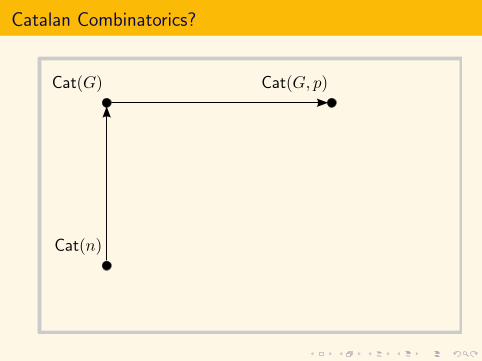
Catalan Combinatorics?

Catalan Combinatorics?
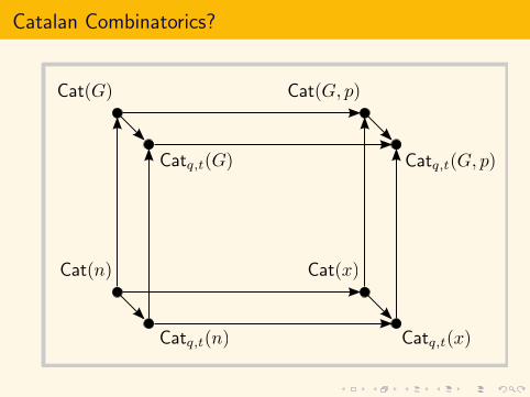
Catalan Combinatorics?

Catalan Combinatorics?
Catalan Combinatorics?
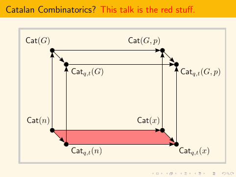
Catalan Combinatorics? This talk is the red stuff.

Introduction to Everything Rational
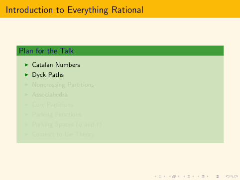
Plan for the Talk
I Catalan Numbers
I Dyck Paths
I Noncrossing Partitions
I Associahedra
I Core Partitions
I Parking Functions
I Parking Spaces (q and t)
I Connect to Lie Theory
Introduction to Everything Rational
Plan for the Talk
I Catalan Numbers
I Dyck Paths
I Noncrossing Partitions
I Associahedra
I Core Partitions
I Parking Functions
I Parking Spaces (q and t)
I Connect to Lie Theory
Introduction to Everything Rational
Plan for the Talk
I Catalan Numbers
I Dyck Paths
I Noncrossing Partitions
I Associahedra
I Core Partitions
I Parking Functions
I Parking Spaces (q and t)
I Connect to Lie Theory

Introduction to Everything Rational
Plan for the Talk
I Catalan Numbers
I Dyck Paths
I Noncrossing Partitions
I Associahedra
I Core Partitions
I Parking Functions
I Parking Spaces (q and t)
I Connect to Lie Theory

Introduction to Everything Rational
Plan for the Talk
I Catalan Numbers
I Dyck Paths
I Noncrossing Partitions
I Associahedra
I Core Partitions
I Parking Functions
I Parking Spaces (q and t)
I Connect to Lie Theory

Introduction to Everything Rational
Plan for the Talk
I Catalan Numbers
I Dyck Paths
I Noncrossing Partitions
I Associahedra
I Core Partitions
I Parking Functions
I Parking Spaces (q and t)
I Connect to Lie Theory

Introduction to Everything Rational
Plan for the Talk
I Catalan Numbers
I Dyck Paths
I Noncrossing Partitions
I Associahedra
I Core Partitions
I Parking Functions
I Parking Spaces (q and t)
I Connect to Lie Theory

Introduction to Everything Rational
Plan for the Talk
I Catalan Numbers
I Dyck Paths
I Noncrossing Partitions
I Associahedra
I Core Partitions
I Parking Functions
I Parking Spaces (q and t)
I Connect to Lie Theory

Rational Catalan Numbers
CONVENTION
Given x ∈ Q \ [−1, 0], there exist unique coprime (a, b) ∈ N2 such that
x =a
b − a.
We will always identify x ↔ (a, b).
Definition
For each x ∈ Q \ [−1, 0] we define the Catalan number:
Cat(x) = Cat(a, b) :=1
a + b
(a + b
a, b
)=
(a + b − 1)!
a!b!.

Rational Catalan Numbers
CONVENTION
Given x ∈ Q \ [−1, 0], there exist unique coprime (a, b) ∈ N2 such that
x =a
b − a.
We will always identify x ↔ (a, b).
Definition
For each x ∈ Q \ [−1, 0] we define the Catalan number:
Cat(x) = Cat(a, b) :=1
a + b
(a + b
a, b
)=
(a + b − 1)!
a!b!.

Rational Catalan Numbers
CONVENTION
Given x ∈ Q \ [−1, 0], there exist unique coprime (a, b) ∈ N2 such that
x =a
b − a.
We will always identify x ↔ (a, b).
Definition
For each x ∈ Q \ [−1, 0] we define the Catalan number:
Cat(x) = Cat(a, b) :=1
a + b
(a + b
a, b
)=
(a + b − 1)!
a!b!.
Special cases
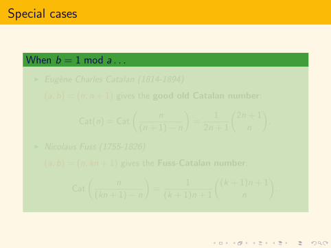
When b = 1 mod a . . .
I Eugene Charles Catalan (1814-1894)
(a, b) = (n, n + 1) gives the good old Catalan number:
Cat(n) = Cat
(n
(n + 1)− n
)=
1
2n + 1
(2n + 1
n
).
I Nicolaus Fuss (1755-1826)
(a, b) = (n, kn + 1) gives the Fuss-Catalan number:
Cat
(n
(kn + 1)− n
)=
1
(k + 1)n + 1
((k + 1)n + 1
n
).

Special cases
When b = 1 mod a . . .
I Eugene Charles Catalan (1814-1894)
(a, b) = (n, n + 1) gives the good old Catalan number:
Cat(n) = Cat
(n
(n + 1)− n
)=
1
2n + 1
(2n + 1
n
).
I Nicolaus Fuss (1755-1826)
(a, b) = (n, kn + 1) gives the Fuss-Catalan number:
Cat
(n
(kn + 1)− n
)=
1
(k + 1)n + 1
((k + 1)n + 1
n
).
Symmetry
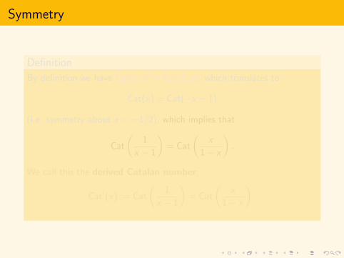
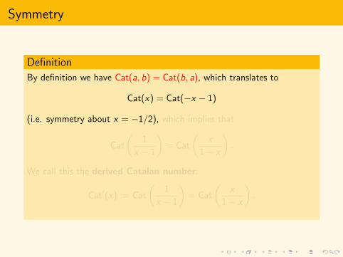
Definition
By definition we have Cat(a, b) = Cat(b, a), which translates to
Cat(x) = Cat(−x − 1)
(i.e. symmetry about x = −1/2), which implies that
Cat
(1
x − 1
)= Cat
(x
1− x
).
We call this the derived Catalan number:
Cat′(x) := Cat
(1
x − 1
)= Cat
(x
1− x
).
Symmetry
Definition
By definition we have Cat(a, b) = Cat(b, a), which translates to
Cat(x) = Cat(−x − 1)
(i.e. symmetry about x = −1/2), which implies that
Cat
(1
x − 1
)= Cat
(x
1− x
).
We call this the derived Catalan number:
Cat′(x) := Cat
(1
x − 1
)= Cat
(x
1− x
).

Symmetry
Definition
By definition we have Cat(a, b) = Cat(b, a), which translates to
Cat(x) = Cat(−x − 1)
(i.e. symmetry about x = −1/2), which implies that
Cat
(1
x − 1
)= Cat
(x
1− x
).
We call this the derived Catalan number:
Cat′(x) := Cat
(1
x − 1
)= Cat
(x
1− x
).

Symmetry
Definition
By definition we have Cat(a, b) = Cat(b, a), which translates to
Cat(x) = Cat(−x − 1)
(i.e. symmetry about x = −1/2), which implies that
Cat
(1
x − 1
)= Cat
(x
1− x
).
We call this the derived Catalan number:
Cat′(x) := Cat
(1
x − 1
)= Cat
(x
1− x
).

Symmetry
Definition
From the same symmetry we also obtain
Cat′(1/x) = Cat
(1
(1/x)− 1
)= Cat
(x
1− x
)= Cat′(x).
We call this rational duality:
Cat′(1/x) = Cat′(x).
(Watch for it later. . . )

Symmetry
Definition
From the same symmetry we also obtain
Cat′(1/x) = Cat
(1
(1/x)− 1
)= Cat
(x
1− x
)= Cat′(x).
We call this rational duality:
Cat′(1/x) = Cat′(x).
(Watch for it later. . . )

Symmetry
Definition
From the same symmetry we also obtain
Cat′(1/x) = Cat
(1
(1/x)− 1
)= Cat
(x
1− x
)= Cat′(x).
We call this rational duality:
Cat′(1/x) = Cat′(x).
(Watch for it later. . . )

Euclidean Algorithm
Observation
The process Cat(x) 7→ Cat′(x) 7→ Cat′′(x) 7→ · · · is a categorification ofthe Euclidean algorithm.
Example: x = 5/3 and (a, b) = (5, 8)
Subtract the smaller from the larger:
Cat(5, 8) = 99,
Cat′(5, 8) = Cat(3, 5) = 7,
Cat′′(5, 8) = Cat′(3, 5) = Cat(2, 3) = 2,
Cat′′′(5, 8) = Cat′′(3, 5) = Cat′(2, 3) = Cat(1, 2) = 1 (STOP)

How to put it in Sloane’s OEIS
Suggestion
The Calkin-Wilf sequence is defined by q1 = 1 and
qn :=1
2bqn−1c − qn−1 + 1.
Theorem: (q1, q2, . . .) = Q>0.Proof: See “Proofs from THE BOOK”, Chapter 17.
Study the function n 7→ Cat(qn).
q 11
12
21
13
32
23
31
14
43
35
52
25
53 · · ·
Cat(q) 1 1 2 1 7 3 5 1 30 15 66 4 99 · · ·

Pause
Well, that was fun.

The Prototype: Rational Dyck Paths

The Prototype: Rational Dyck Paths
I Consider the “Dyck paths” in an a× b rectangle.
Example (a, b) = (5, 8)

The Prototype: Rational Dyck Paths
I Again let x = a/(b − a) with a, b positive and coprime.
Example (a, b) = (5, 8)

The Prototype: Rational Dyck Paths
I Let D(x) = D(a, b) denote the set of Dyck paths.
Example (a, b) = (5, 8)

The Prototype: Rational Dyck Paths
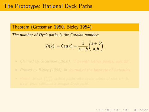
Theorem (Grossman 1950, Bizley 1954)
The number of Dyck paths is the Catalan number:
|D(x)| = Cat(x) =1
a + b
(a + b
a, b
).
I Claimed by Grossman (1950), “Fun with lattice points, part 22”.
I Proved by Bizley (1954), in Journal of the Institute of Actuaries.
I Proof: Break(a+ba,b
)lattice paths into cyclic orbits of size a + b.
Each orbit contains a unique Dyck path.
The Prototype: Rational Dyck Paths
Theorem (Grossman 1950, Bizley 1954)
The number of Dyck paths is the Catalan number:
|D(x)| = Cat(x) =1
a + b
(a + b
a, b
).
I Claimed by Grossman (1950), “Fun with lattice points, part 22”.
I Proved by Bizley (1954), in Journal of the Institute of Actuaries.
I Proof: Break(a+ba,b
)lattice paths into cyclic orbits of size a + b.
Each orbit contains a unique Dyck path.

The Prototype: Rational Dyck Paths
Theorem (Armstrong 2010, Loehr 2010)
I The number of Dyck paths with k vertical runs equals
Nar(x ; k) :=1
a
(a
k
)(b − 1
k − 1
).
Call these the Narayana numbers.
I And the number with rj vertical runs of length j equals
Krew(x ; r) :=1
b
(b
r0, r1, . . . , ra
)=
(b − 1)!
r0!r1! · · · ra!.
Call these the Kreweras numbers.

Next: Rational NC Partitions
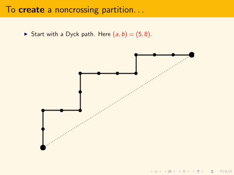
To create a noncrossing partition. . .
I Start with a Dyck path. Here (a, b) = (5, 8).

To create a noncrossing partition. . .
I Label the internal vertices by {1, 2, . . . , a + b − 1}.

To create a noncrossing partition. . .
I Shoot lasers from the bottom left with slope a/b.

To create a noncrossing partition. . .
I Who can see each other?

To create a noncrossing partition. . .
I There you go!

To create a noncrossing partition. . .
I We have created Cat(x) = 1a
(a+ba,b
)different noncrossing partitions of
the cycle [a + b − 1], and each of them has a blocks.

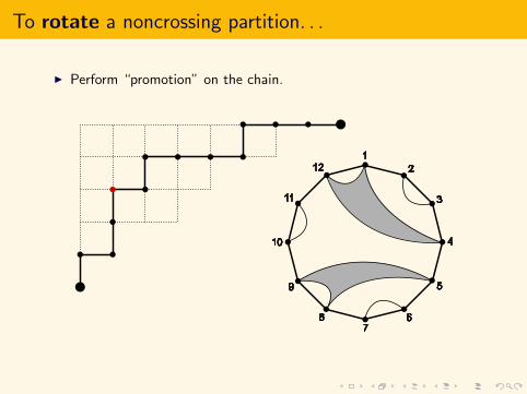
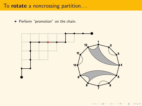
To rotate a noncrossing partition. . .
I Q: What does “rotation” of the partition correspond to?

To rotate a noncrossing partition. . .
I A: Think of the path as a maximal chain in a poset.

To rotate a noncrossing partition. . .
I Perform “promotion” on the chain.

To rotate a noncrossing partition. . .
I Perform “promotion” on the chain.

To rotate a noncrossing partition. . .
I Perform “promotion” on the chain.

To rotate a noncrossing partition. . .
I Perform “promotion” on the chain.

To rotate a noncrossing partition. . .
I Perform “promotion” on the chain.
To rotate a noncrossing partition. . .
I Perform “promotion” on the chain.

To rotate a noncrossing partition. . .
I Perform “promotion” on the chain.

To rotate a noncrossing partition. . .
I Perform “promotion” on the chain.

To rotate a noncrossing partition. . .
I Perform “promotion” on the chain.
To rotate a noncrossing partition. . .
I Perform “promotion” on the chain.

To rotate a noncrossing partition. . .
I Perform “promotion” on the chain.

To rotate a noncrossing partition. . .
I Perform “promotion” on the chain.

To rotate a noncrossing partition. . .
I Perform “promotion” on the chain.

To rotate a noncrossing partition. . .
I Perform “promotion” on the chain.

To rotate a noncrossing partition. . .
I Perform “promotion” on the chain.

To rotate a noncrossing partition. . .
I Perform “promotion” on the chain.

To rotate a noncrossing partition. . .
I Perform “promotion” on the chain.

To rotate a noncrossing partition. . .
I Think of it as a path again.

To rotate a noncrossing partition. . .
I Again the lasers.

To rotate a noncrossing partition. . .
I And there you go!

To rotate a noncrossing partition. . .
I Drew: mention the case (a, b) = (n, (k − 1)n + 1).
A Few Facts

A Few Facts
Definition
For (a, b) coprime, consider the triangle poset
T (a, b) := {(x , y) ∈ Z2 : y ≤ a, x ≤ b, yb − xa ≥ 0}.
As you see here.

A Few Facts
Results (with Nathan Williams)
I Promotion on T (a, b) has order a + b − 1.
I Conjecture: The number of chains invariant under promotiond is theq-Catalan number evaluated at a root of unity:
1
[a + b]q
[a + b
a, b
]q
∣∣∣∣∣q=e
2πida+b−1
!
I T (n, n + 1) is related to the type A root poset.
I D.White, Panyushev, Striker-Williams, A-Stump-Thomas.

Next: Rational NC Partition Posets
Observation
Our rational NC partitions don’t form a nice poset. Indeed, they eachhave the same number of blocks! (i.e., a)
Question
Can one define a nice poset of rational NC partitions?
Answer
Yes.

Next: Rational NC Partition Posets
Observation
Our rational NC partitions don’t form a nice poset. Indeed, they eachhave the same number of blocks! (i.e., a)
Question
Can one define a nice poset of rational NC partitions?
Answer
Yes.

Next: Rational NC Partition Posets
Observation
Our rational NC partitions don’t form a nice poset. Indeed, they eachhave the same number of blocks! (i.e., a)
Question
Can one define a nice poset of rational NC partitions?
Answer
Yes.

Next: Rational NC Partition Posets
Observation
Our rational NC partitions don’t form a nice poset. Indeed, they eachhave the same number of blocks! (i.e., a)
Question
Can one define a nice poset of rational NC partitions?
Answer
Yes.
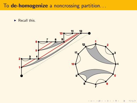
To de-homogenize a noncrossing partition. . .
I Recall this.

To de-homogenize a noncrossing partition. . .
I Now we label only the horizontal steps.

To de-homogenize a noncrossing partition. . .
I Now we label only the horizontal steps.

To de-homogenize a noncrossing partition. . .
I Now we shoot lasers only from the corners.

To de-homogenize a noncrossing partition. . .
I Now who can see each other?
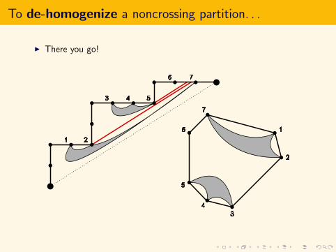
To de-homogenize a noncrossing partition. . .
I There you go!

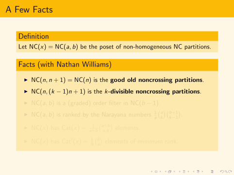
A Few Facts
Definition
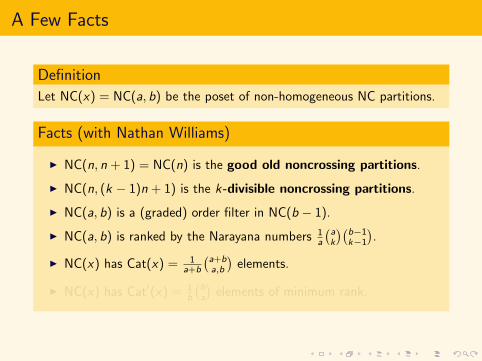
Let NC(x) = NC(a, b) be the poset of non-homogeneous NC partitions.
Facts (with Nathan Williams)
I NC(n, n + 1) = NC(n) is the good old noncrossing partitions.
I NC(n, (k − 1)n + 1) is the k-divisible noncrossing partitions.
I NC(a, b) is a (graded) order filter in NC(b − 1).
I NC(a, b) is ranked by the Narayana numbers 1a
(ak
)(b−1k−1
).
I NC(x) has Cat(x) = 1a+b
(a+ba,b
)elements.
I NC(x) has Cat′(x) = 1b
(ba
)elements of minimum rank.

A Few Facts
Definition
Let NC(x) = NC(a, b) be the poset of non-homogeneous NC partitions.
Facts (with Nathan Williams)
I NC(n, n + 1) = NC(n) is the good old noncrossing partitions.
I NC(n, (k − 1)n + 1) is the k-divisible noncrossing partitions.
I NC(a, b) is a (graded) order filter in NC(b − 1).
I NC(a, b) is ranked by the Narayana numbers 1a
(ak
)(b−1k−1
).
I NC(x) has Cat(x) = 1a+b
(a+ba,b
)elements.
I NC(x) has Cat′(x) = 1b
(ba
)elements of minimum rank.

Rational Duality
I Note that x ↔ 1/x is the same as (a < b)↔ (b − a < b).

Next: Rational Associahedra
Observation
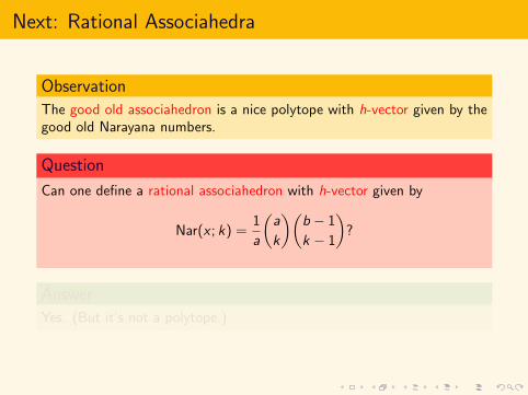
The good old associahedron is a nice polytope with h-vector given by thegood old Narayana numbers.
Question
Can one define a rational associahedron with h-vector given by
Nar(x ; k) =1
a
(a
k
)(b − 1
k − 1
)?
Answer
Yes. (But it’s not a polytope.)

Next: Rational Associahedra
Observation
The good old associahedron is a nice polytope with h-vector given by thegood old Narayana numbers.
Question
Can one define a rational associahedron with h-vector given by
Nar(x ; k) =1
a
(a
k
)(b − 1
k − 1
)?
Answer
Yes. (But it’s not a polytope.)
Next: Rational Associahedra
Observation
The good old associahedron is a nice polytope with h-vector given by thegood old Narayana numbers.
Question
Can one define a rational associahedron with h-vector given by
Nar(x ; k) =1
a
(a
k
)(b − 1
k − 1
)?
Answer
Yes. (But it’s not a polytope.)

Next: Rational Associahedra
Observation
The good old associahedron is a nice polytope with h-vector given by thegood old Narayana numbers.
Question
Can one define a rational associahedron with h-vector given by
Nar(x ; k) =1
a
(a
k
)(b − 1
k − 1
)?
Answer
Yes. (But it’s not a polytope.)

To create a polygon dissection. . .
I Start with a Dyck path. Here (a, b) = (5, 8).

To create a polygon dissection. . .
I Label the columns by {1, 2, . . . , b + 1}.

To create a polygon dissection. . .
I Shoot some lasers from the bottom left with slope a/b.

To create a polygon dissection. . .
I Lift the lasers up.

To create a polygon dissection. . .
I There you go!

To create a polygon dissection. . .
I We have created Cat(x) = 1a
(a+ba,b
)different “rational dissections” of
the cycle [b + 1], and each of them has a diagonals.

A Few Facts
Definition
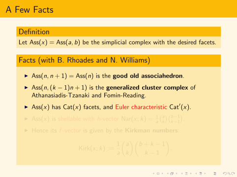
Let Ass(x) = Ass(a, b) be the simplicial complex with the desired facets.
Facts (with B. Rhoades and N. Williams)
I Ass(n, n + 1) = Ass(n) is the good old associahedron.
I Ass(n, (k − 1)n + 1) is the generalized cluster complex ofAthanasiadis-Tzanaki and Fomin-Reading.
I Ass(x) has Cat(x) facets, and Euler characteristic Cat′(x).
I Ass(x) is shellable with h-vector Nar(x ; k) = 1a
(ak
)(b−1k−1
).
I Hence its f -vector is given by the Kirkman numbers:
Kirk(x ; k) :=1
a
(a
k
)(b + k − 1
k − 1
).

A Few Facts
Definition
Let Ass(x) = Ass(a, b) be the simplicial complex with the desired facets.
Facts (with B. Rhoades and N. Williams)
I Ass(n, n + 1) = Ass(n) is the good old associahedron.
I Ass(n, (k − 1)n + 1) is the generalized cluster complex ofAthanasiadis-Tzanaki and Fomin-Reading.
I Ass(x) has Cat(x) facets, and Euler characteristic Cat′(x).
I Ass(x) is shellable with h-vector Nar(x ; k) = 1a
(ak
)(b−1k−1
).
I Hence its f -vector is given by the Kirkman numbers:
Kirk(x ; k) :=1
a
(a
k
)(b + k − 1
k − 1
).

Rational Duality = Alexander Duality
I E.g. Ass(2/3) and Ass(3/2) are Alexander dual inside Ass(4).

Motivation: Core Partitions

Motivation: Core Partitions
Definition
Let λ ` n be an integer partition of “size” n.
I Say λ is a p-core if it has no cell with hook length p.
I Say λ is an (a, b)-core if it has no cell with hook length a or b.
Example
The partition (5, 4, 2, 1, 1) ` 13 is a (5, 8)-core.

Motivation: Core Partitions
Theorem (Anderson 2002)
The number of (a, b)-cores (of any size) is finite if and only if (a, b) arecoprime, in which case they are counted by the Catalan number
Cat(a, b) =1
a + b
(a + b
a, b
).
Theorem (Olsson-Stanton 2005, Vandehey 2008)
For (a, b) coprime ∃ unique largest (a, b)-core of size (a2−1)(b2−1)24 , which
contains all others as subdiagrams.
Suggestion
Study Young’s lattice restricted to (a, b)-cores.

Motivation: Core Partitions
Example: The poset of (3, 4)-cores.

Motivation: Core Partitions
Theorem (Ford-Mai-Sze 2009)
For a, b coprime, the number of self-conjugate (a, b)-cores is(b a
2 c+bb2 c
b a2 c,b
b2 c
).
Note: Beautiful bijective proof! (omitted)
Observation/Problem(b a2c+ b b
2 cb a
2c, bb2 c
)=
1
[a + b]q
[a + b
a, b
]q
∣∣∣∣∣q=−1
Conjecture (Armstrong 2011)
The average size of an (a, b)-core and the average size of a self-conjugate
(a, b)-core are both equal to (a+b+1)(a−1)(b−1)24 .
Anderson’s Beautiful Proof
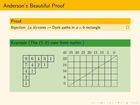
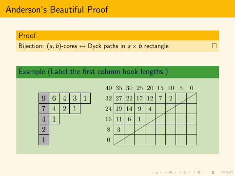
Proof.
Bijection: (a, b)-cores ↔ Dyck paths in a× b rectangle
Example (The (5, 8)-core from earlier.)

Anderson’s Beautiful Proof
Proof.
Bijection: (a, b)-cores ↔ Dyck paths in a× b rectangle
Example (Label the rectangle cells by “height”.)
Anderson’s Beautiful Proof
Proof.
Bijection: (a, b)-cores ↔ Dyck paths in a× b rectangle
Example (Label the first column hook lengths.)
Anderson’s Beautiful Proof
Proof.
Bijection: (a, b)-cores ↔ Dyck paths in a× b rectangle
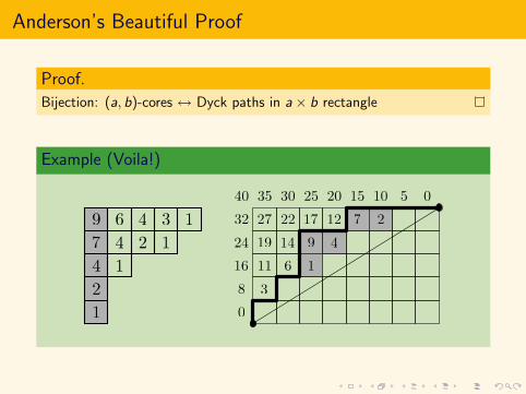
Example (Voila!)

Anderson’s Beautiful Proof
Proof.
Bijection: (a, b)-cores ↔ Dyck paths in a× b rectangle
Example (Observe: Conjugation is a bit strange.)
Next: Rational Parking Functions/Spaces

The Rational Parking Space
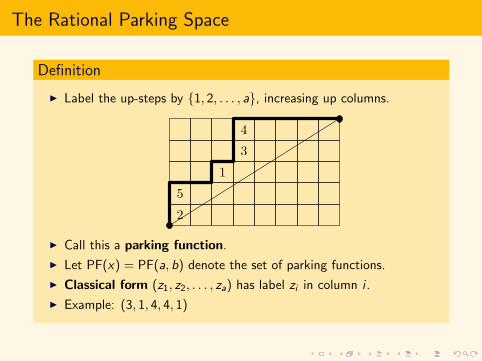
Definition
I Label the up-steps by {1, 2, . . . , a}, increasing up columns.
I Call this a parking function.
I Let PF(x) = PF(a, b) denote the set of parking functions.
I Classical form (z1, z2, . . . , za) has label zi in column i .
I Example: (3, 1, 4, 4, 1)

The Rational Parking Space
Definition
I Label the up-steps by {1, 2, . . . , a}, increasing up columns.
I Call this a parking function.
I Let PF(x) = PF(a, b) denote the set of parking functions.
I Classical form (z1, z2, . . . , za) has label zi in column i .
I Example: (3, 1, 4, 4, 1)

The Rational Parking Space
Definition
I Label the up-steps by {1, 2, . . . , a}, increasing up columns.
I Call this a parking function.
I Let PF(x) = PF(a, b) denote the set of parking functions.
I Classical form (z1, z2, . . . , za) has label zi in column i .
I Example: (3, 1, 4, 4, 1)

The Rational Parking Space
Definition
I Label the up-steps by {1, 2, . . . , a}, increasing up columns.
I Call this a parking function.
I Let PF(x) = PF(a, b) denote the set of parking functions.
I Classical form (z1, z2, . . . , za) has label zi in column i .
I Example: (3, 1, 4, 4, 1)
The Rational Parking Space
Definition
I Label the up-steps by {1, 2, . . . , a}, increasing up columns.
I Call this a parking function.
I Let PF(x) = PF(a, b) denote the set of parking functions.
I Classical form (z1, z2, . . . , za) has label zi in column i .
I Example: (3, 1, 4, 4, 1)

The Rational Parking Space
Definition
I The symmetric group Sa acts on classical forms.
I Example: (3, 1, 4, 4, 1) versus (3, 1, 1, 4, 4)
I By abuse, let PF(x) = PF(a, b) denote this representation of Sa.
I Call it the rational parking space.

The Rational Parking Space
Definition
I The symmetric group Sa acts on classical forms.
I Example: (3, 1, 4, 4, 1) versus (3, 1, 1, 4, 4)
I By abuse, let PF(x) = PF(a, b) denote this representation of Sa.
I Call it the rational parking space.

The Rational Parking Space
Definition
I The symmetric group Sa acts on classical forms.
I Example: (3, 1, 4, 4, 1) versus (3, 1, 1, 4, 4)
I By abuse, let PF(x) = PF(a, b) denote this representation of Sa.
I Call it the rational parking space.

The Rational Parking Space
Definition
I The symmetric group Sa acts on classical forms.
I Example: (3, 1, 4, 4, 1) versus (3, 1, 1, 4, 4)
I By abuse, let PF(x) = PF(a, b) denote this representation of Sa.
I Call it the rational parking space.

The Rational Parking Space
Definition
I The symmetric group Sa acts on classical forms.
I Example: (3, 1, 4, 4, 1) versus (3, 1, 1, 4, 4)
I By abuse, let PF(x) = PF(a, b) denote this representation of Sa.
I Call it the rational parking space.

A Few Facts
Theorems (with N. Loehr and N. Williams)
I The dimension of PF(a, b) is ba−1.
I The complete homogeneous expansion is
PF(a, b) =∑r`a
1
b
(b
r0, r1, . . . , ra
)hr,
where the sum is over r = 0r01r1 · · · ara ` a with∑
i ri = b.
I That is: PF(a, b) is the coefficient of ta in 1b H(t)b, where
H(t) = h0 + h1t + h2t2 + · · · .

A Few Facts
Theorems (with N. Loehr and N. Williams)
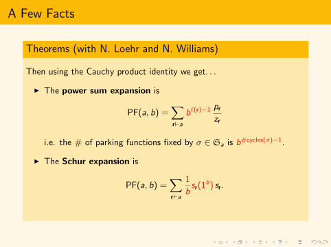
Then using the Cauchy product identity we get. . .
I The power sum expansion is
PF(a, b) =∑r`a
b`(r)−1 pr
zr
i.e. the # of parking functions fixed by σ ∈ Sa is b#cycles(σ)−1.
I The Schur expansion is
PF(a, b) =∑r`a
1
bsr(1b) sr.

A Few Facts
Theorems (with N. Loehr and N. Williams)
Then using the Cauchy product identity we get. . .
I The power sum expansion is
PF(a, b) =∑r`a
b`(r)−1 pr
zr
i.e. the # of parking functions fixed by σ ∈ Sa is b#cycles(σ)−1.
I The Schur expansion is
PF(a, b) =∑r`a
1
bsr(1b) sr.
A Few Facts
Theorems (with N. Loehr and N. Williams)
Then using the Cauchy product identity we get. . .
I The power sum expansion is
PF(a, b) =∑r`a
b`(r)−1 pr
zr
i.e. the # of parking functions fixed by σ ∈ Sa is b#cycles(σ)−1.
I The Schur expansion is
PF(a, b) =∑r`a
1
bsr(1b) sr.

A Few Facts
Observation/Definition
The multiplicities of the hook Schur functions s[k + 1, 1a−k−1] inPF(a, b) are given by the Schroder numbers
Schro(a, b; k) :=1
bs[k+1,1a−k−1](1b) =
1
b
(a− 1
k
)(b + k
a
).
Special Cases:
I Trivial character: Schro(a, b; a− 1) = Cat(a, b).
I Smallest k that occurs is k = max{0, a− b}, in which case
Schro(a, b; k) = Cat′(a, b).
I Hence Schro(x ; k) interpolates between Cat(x) and Cat′(x).

Rational Duality
Problem
Given a, b coprime we have an Sa-module PF(a, b) of dimension ba−1
and an Sb-module PF(b, a) of dimension ab−1.
I What is the relationship between PF(a, b) and PF(b, a)?
I Note that hook multiplicities are the same:
Schro(a, b; k) = Schro(b, a; k + b − a).
I See Eugene Gorsky, Arc spaces and DAHA representations, 2011.

Summary of Catalan Refinements
I The Kirkman/Narayana/Schroder numbers are equivalent. Theycontain information about rank. (1 < k < a− 1)
Kirk(x ; k) = 1a
(ak
)(b+k−1k−1
)Nar(x ; k) = 1
a
(ak
)(b−1k−1
)Schro(x ; k) = 1
b
(a−1k
)(b+k
a
)
f -vector
h-vector
“dual” f -vector
I The Kreweras numbers are more refined. They contain parabolicinformation. (r ` a)
Krew(x ; r) =1
b
(b
r0, r1, . . . , ra
)

Finally: How about q and t?
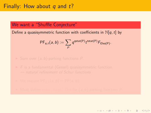
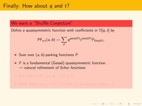
We want a “Shuffle Conjecture”
Define a quasisymmetric function with coefficients in N[q, t] by
PFq,t(a, b) :=∑P
qqstat(P)ttstat(P)FiDes(P).
I Sum over (a, b)-parking functions P.
I F is a fundamental (Gessel) quasisymmetric function.— natural refinement of Schur functions
I We require PF1,1(a, b) = PF(a, b).
I Must define qstat, tstat, iDes for (a, b)-parking function P.
Finally: How about q and t?
We want a “Shuffle Conjecture”
Define a quasisymmetric function with coefficients in N[q, t] by
PFq,t(a, b) :=∑P
qqstat(P)ttstat(P)FiDes(P).
I Sum over (a, b)-parking functions P.
I F is a fundamental (Gessel) quasisymmetric function.— natural refinement of Schur functions
I We require PF1,1(a, b) = PF(a, b).
I Must define qstat, tstat, iDes for (a, b)-parking function P.
qstat is easy
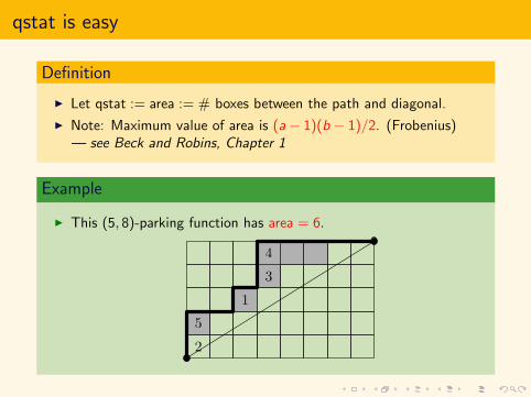
Definition
I Let qstat := area := # boxes between the path and diagonal.
I Note: Maximum value of area is (a− 1)(b − 1)/2. (Frobenius)— see Beck and Robins, Chapter 1
Example
I This (5, 8)-parking function has area = 6.
iDes is reasonable
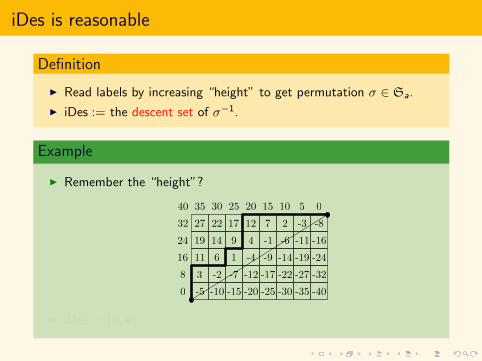
Definition
I Read labels by increasing “height” to get permutation σ ∈ Sa.
I iDes := the descent set of σ−1.
Example
I Remember the “height”?
I iDes = {1, 4}

iDes is reasonable
Definition
I Read labels by increasing “height” to get permutation σ ∈ Sa.
I iDes := the descent set of σ−1.
Example
I Look at the heights of the vertical step boxes.
I iDes = {1, 4}

iDes is reasonable
Definition
I Read labels by increasing “height” to get permutation σ ∈ Sa.
I iDes := the descent set of σ−1.
Example
I Remember the labels we had before.
I iDes = {1, 4}

iDes is reasonable
Definition
I Read labels by increasing “height” to get permutation σ ∈ Sa.
I iDes := the descent set of σ−1.
Example
I Read them by increasing height to get σ = 21534 ∈ S5.
I iDes = {1, 4}

tstat is hard (as usual)
Definition
I “Blow up” the (a, b)-parking function.
I Compute “dinv” of the blowup.
Example
I Recall our favorite the (5, 8)-parking function.

tstat is hard (as usual)
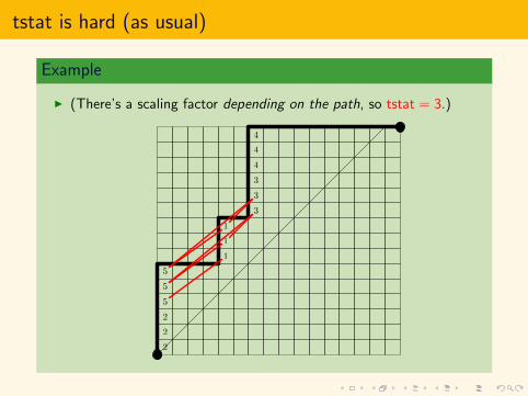
Definition
I “Blow up” the (a, b)-parking function.
I Compute “dinv” of the blowup.
Example
I Since 2 · 8− 3 · 5 = 1 we “blow up” by 2 horiz. and 3 vert....

tstat is hard (as usual)
Example
I To get this!

tstat is hard (as usual)
Example
I To get this! Now compute dinv = 7.
tstat is hard (as usual)
Example
I (There’s a scaling factor depending on the path, so tstat = 3.)

All Together
Example
I So our favorite (5, 8)-parking function contributes q6t3F{1,4}.
I Proof of Concept: The coefficient of s[2, 2, 1] in PFq,t(5, 8) is
1 1 1 1 11 3 4 3 2 1
2 6 6 4 2 12 7 7 4 2 1
1 6 7 4 2 13 6 4 2 1
1 4 4 2 11 3 2 11 2 11 11

All Together
Example
I So our favorite (5, 8)-parking function contributes q6t3F{1,4}.
I Proof of Concept: The coefficient of s[2, 2, 1] in PFq,t(5, 8) is
1 1 1 1 11 3 4 3 2 1
2 6 6 4 2 12 7 7 4 2 1
1 6 7 4 2 13 6 4 2 1
1 4 4 2 11 3 2 11 2 11 11

A Few Facts
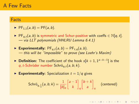
Facts
I PF1,1(a, b) = PF(a, b).
I PFq,t(a, b) is symmetric and Schur-positive with coeffs ∈ N[q, t].— via LLT polynomials (HHLRU Lemma 6.4.1)
I Experimentally: PFq,t(a, b) = PFt,q(a, b).— this will be “impossible” to prove (see Loehr’s Maxim)
I Definition: The coefficient of the hook s[k + 1, 1a−k−1] is theq, t-Schroder number Schroq,t(a, b; k).
I Experimentally: Specialization t = 1/q gives
Schroq, 1q(a, b; k) =
1
[b]q
[a− 1
k
]q
[b + k
a
]q
(centered)

A Few Facts
Facts
I PF1,1(a, b) = PF(a, b).
I PFq,t(a, b) is symmetric and Schur-positive with coeffs ∈ N[q, t].— via LLT polynomials (HHLRU Lemma 6.4.1)
I Experimentally: PFq,t(a, b) = PFt,q(a, b).— this will be “impossible” to prove (see Loehr’s Maxim)
I Definition: The coefficient of the hook s[k + 1, 1a−k−1] is theq, t-Schroder number Schroq,t(a, b; k).
I Experimentally: Specialization t = 1/q gives
Schroq, 1q(a, b; k) =
1
[b]q
[a− 1
k
]q
[b + k
a
]q
(centered)

Epilogue: Lie Theory
Epilogue: Lie Theory
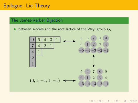
The James-Kerber Bijection
I between a-cores and the root lattice of the Weyl group Sa

Epilogue: Lie Theory
I These are the root and weight lattices Q ⊆ Λ of Sa.

Epilogue: Lie Theory
I Here is a fundamental parallelepiped for Λ/bΛ.

Epilogue: Lie Theory
I It contains ba−1 elements (these are the “parking functions”).

Epilogue: Lie Theory
I But they look better as a simplex...

Epilogue: Lie Theory
I ...which is congruent to a nicer simplex.

Epilogue: Lie Theory
I There are Cat(a, b) = 1a+b
(a+ba,b
)elements of the root lattice inside.

Epilogue: Lie Theory
I These are the (a, b)-Dyck paths (via Anderson, James-Kerber).
Other Weyl Groups?
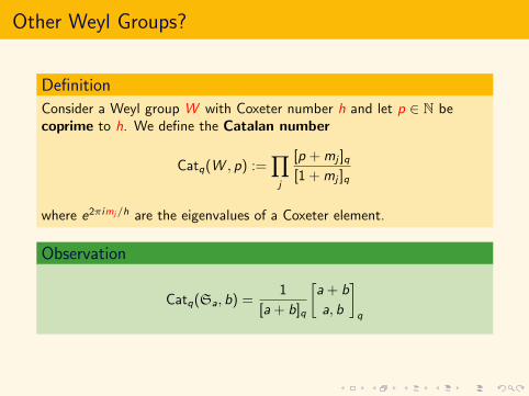
Definition
Consider a Weyl group W with Coxeter number h and let p ∈ N becoprime to h. We define the Catalan number
Catq(W , p) :=∏
j
[p + mj ]q[1 + mj ]q
where e2πimj/h are the eigenvalues of a Coxeter element.
Observation
Catq(Sa, b) =1
[a + b]q
[a + b
a, b
]q

Here’s to a Productive Workshop


![Notes on the Catalan problem - scarpaz.com Mathematics... · Daniele Paolo Scarpazza Notes on the Catalan problem [1] An overview of Catalan problems • Catalan numbers appear as](https://img.dokumen.tips/doc/110x75/5b8526687f8b9ad34a8d9e0d/notes-on-the-catalan-problem-mathematics-daniele-paolo-scarpazza-notes.jpg)


![Analytic combinatorics: functional equations, rational and ... · in simple families of trees [41, 42] relate to analytic iteration theory. On another register, metric properties](https://img.dokumen.tips/doc/110x75/5f64702dbd608b0c17044808/analytic-combinatorics-functional-equations-rational-and-in-simple-families.jpg)