Rapid Detection of Significant Spatial Clusters

Daniel B. Neill

Andrew W. Moore

The Auton LabCarnegie Mellon University School of Computer Science

E-mail: {neill, awm}@cs.cmu.edu

Introduction

• Goals of data mining:– Discover patterns in data.– Distinguish patterns that are significant from those that

are likely to have occurred by chance. • For example:

– In epidemiology, a rise in the number of disease cases in a region may or may not be indicative of an emerging epidemic.

– In brain imaging, an increase in measured fMRI activation may or may not represent a real increase in brain activity.

This is why significance testing is important!

Problem overview

• Assume data has been aggregated to an N x N grid.

• Each grid cell sij has a count cij and a population pij.

• Our goal is to find overdensities: spatial regions where the counts are significantly higher than expected, given the underlying population.

P=5000

C=27

P=3500

C=14

P=4500

C=22

P=3000

C=15

P=1000

C=5

P=5000

C=26

P=4000

C=17

P=3000

C=12

P=2000

C=12

P=1000

C=4

P=5000

C=19

P=5008

C=25

P=4000

C=43

P=3000

C=37

P=4000

C=20

P=4800

C=18

P=4800

C=20

P=4000

C=40

P=3000

C=22

P=4000

C=16

P=4700

C=20

P=3000

C=13

P=3000

C=18

P=2000

C=20

P=1000

C=4Underlying population

of cell

Count of cell

This region has an overdensity of counts.

Application domains• In epidemiology:

– Counts cij represent number of disease cases in a region, or some related observable quantity (Emergency Department visits, sales of OTC medications).

– Populations pij can be obtained from census data or historical counts (e.g. past OTC sales).

• In brain imaging:– Counts cij represent fMRI

activation in a given voxel.– Populations pij represent baseline

activation under null condition.

• Also applicable to other domains, e.g. astrophysics, surveillance.

Application domains• In epidemiology:

– Counts cij represent number of disease cases in a region, or some related observable quantity (Emergency Department visits, sales of OTC medications).

– Populations pij can be obtained from census data or historical counts (e.g. past OTC sales).

• In brain imaging:– Counts cij represent fMRI

activation in a given voxel.– Populations pij represent baseline

activation under null condition.

• Also applicable to other domains, e.g. astrophysics, surveillance.

Goal: find clusters of disease cases, allowing

early detection of epidemics.

Application domains• In epidemiology:

– Counts cij represent number of disease cases in a region, or some related observable quantity (Emergency Department visits, sales of OTC medications).

– Populations pij can be obtained from census data or historical counts (e.g. past OTC sales).

• In brain imaging:– Counts cij represent fMRI

activation in a given voxel.– Populations pij represent baseline

activation under null condition.

• Also applicable to other domains, e.g. astrophysics, surveillance.

fMRI picturegoes here

Application domains• In epidemiology:

– Counts cij represent number of disease cases in a region, or some related observable quantity (Emergency Department visits, sales of OTC medications).

– Populations pij can be obtained from census data or historical counts (e.g. past OTC sales).

• In brain imaging:– Counts cij represent fMRI

activation in a given voxel.– Populations pij represent baseline

activation under null condition.

• Also applicable to other domains, e.g. astrophysics, surveillance.

Goal: find clusters of brain activity corresponding

to given cognitive tasks.

Problem overview• To detect overdensities:

– Find the most significant spatial regions.

– Calculate statistical significance of these regions.

• We focus here on finding the single most significant rectangular region S* (and its p-value).– If p-value > α, no significant

clusters exist at level α.– If p-value < α, then S* is

significant; we can then examine secondary clusters.

P=5000

C=27

P=3500

C=14

P=4500

C=22

P=3000

C=15

P=1000

C=5

P=5000

C=26

P=4000

C=17

P=3000

C=12

P=2000

C=12

P=1000

C=4

P=5000

C=19

P=5008

C=25

P=4000

C=43

P=3000

C=37

P=4000

C=20

P=4800

C=18

P=4800

C=20

P=4000

C=40

P=3000

C=22

P=4000

C=16

P=4700

C=20

P=3000

C=13

P=3000

C=18

P=2000

C=20

P=1000

C=4

Why rectangular regions?• We typically expect clusters to

be convex; thus inner/outer bounding boxes are reasonably close approximations to shape.

• We can find clusters with high aspect ratios.– Important in epidemiology

since disease clusters are often elongated (e.g. from windborne pathogens).

– Important in brain imaging because of the brain’s “folded sheet” structure.

• We can find non-axis-aligned rectangles by examining multiple rotations of the data.

Calculating significance

• Define models:– of the null hypothesis H0 (no clusters). – of the alternative hypothesis H1 (at least one

cluster).

• Derive a score function D(S) = D(C, P).– Likelihood ratio: D(S) = L(Data | H1(S)) / L(Data

| H0).– To find the most significant region: S* = arg maxS

D(S).

Example: Kulldorff’s statistic

• Kulldorff’s spatial scan statistic (1997) is individually most powerful for finding a single region of elevated disease rate.

• Given a region with uniform disease rate q inside the region and q’ < q outside, this test is most likely to detect the cluster.

• Find the region with the maximum value of the (log-) likelihood ratio statistic:

q = .02

q’ = .01

tot

tottot

tot

tottotK

P

CC

PP

CCCC

P

CCSD loglog)(log)(

Assumption: cij ~ Po(qpij)

Properties of D(S)

Pop1000

Count5 Pop

1000

Count500

D(S) is increasing with the total count of S, C(S) = ∑S cij.

z z z

! ! !

Properties of D(S)

D(S) is decreasing with the total population of S, P(S) = ∑S pij.

z z z

! ! !

Pop1 million

Count500 Pop

1000

Count500

Properties of D(S)

For a constant ratio C / P, D(S) is increasing with P.

z z z

! ! !

Pop4

Count1

Pop4000

Count1000

Multiple hypothesis testing

• Problem with testing significance: we are simultaneously testing a huge number of regions (>1 billion for a 256 x 256 grid), asking if any of them are significant.

• If the null hypothesis is true (i.e. no clusters exist), regions’ p-values will be uniformly distributed on [0, 1]:

– We expect the p-value to be less than .05, 5% of the time.

– So we expect 50 million false positives! *

– Moreover, the lowest of these p-values (i.e. the p-value of the most significant region) is almost certain to be less than .05.

* Give or take, depending on correlations between region scores… but at least 65,536 of the tests are independent.

The solution: randomization testing

1. Randomly generate a replica grid G’ under the null hypothesis of no clusters.• For example, for Kulldorff’s statistic, the replica has the same

populations p_ij as grid G, but all counts generated randomly with uniform disease rate.

2. Compute the maximum value of D(S) for the replica G’, and compare to the maximum value of D(S) for the original grid G. • If Dmax(G’) > Dmax(G), the replica grid beats the original.

3. Repeat steps 1-2 for a large number R of replica grids (typically R = 1000).

4. The p-value is the proportion of replicas G’ beating G.• Statistically significant if p-value < α.

Why spatial scan?

• Previous approaches typically find individual high-density cells and aggregate them using some heuristic method; we search over regions to find the ones which are globally optimal (maximize the score function corresponding to some model).– Clusters found by previous approaches are typically not optimal in

any well-defined sense; also, no conclusions can be drawn about the significance of the region as a whole.

• Detecting regions rather than aggregating single cells allows us to be more sensitive to even small (but significant) changes in density, if they are sufficiently large in spatial extent.

Why spatial scan?

• The spatial scan statistics framework is both general and powerful:– Simply choose a model (null and alternative hypotheses to test), derive the

corresponding score function D(S) , and apply the spatial scan to find the globally optimal cluster with respect to this score function.

– Assuming the score function has been chosen properly (i.e. likelihood ratio), we will (under certain conditions) have an individually most powerful test with respect to the model.

• In addition to finding the most significant region, we also compute the significance (p-value) of that region, correctly adjusting for multiple hypothesis testing.

– Thus we have a guaranteed bound on false positive rate given the null hypothesis. • The spatial scan adjusts for variable underlying populations p_ij instead of

simply searching for regions of high count.• The main disadvantage: computational intractability!

– Requires searching over all spatial regions: both for the original grid and many replicas!

This is our motivation for finding a fast spatial scan algorithm!

A naïve spatial scan approach

• Search all O(N4) rectangular regions, return the highest value of the scan statistic.– We can use the old “cumulative counts” trick to find the

score of any region in O(1), so we can search in O(N4).

– But in order to perform randomization testing, we must do the same for each replica grid, giving us total complexity O(RN4).

• This is much too slow for real-time detection!

For a 256 x 256 grid, with 1000 replications:

1.03 trillion regions to search 14-45 days!

How to speed up our search?

• Use a space-partitioning tree?– Problem: many subregions of a region

are not contained entirely in either “child,” but overlap partially with each.

• Option #1: search recursively, but at each node also search all of these “shared” regions.– Problem: There are O(N4) such regions

even at the top level of the tree!

• Option #2: find “pieces” of the region, and merge bottom-up.– Problem: combined region may be

more significant than either piece.

The solution: Overlap-multiresolution partitioning• We propose a partitioning approach in which

adjacent regions are allowed to partially overlap. • The basic idea is to:

– Divide the grid into overlapping regions.– Bound the maximum score of subregions contained in

each region.– Prune regions which cannot contain the most

significant region.– Find the same region and p-value as the naïve

approach… but hundreds or thousands of times faster!

Overlap-multires partitioning• Parent region S is divided into four

overlapping children: “left child” S1, “right child” S2, “upper child” S3, and “lower child” S4.

• Then for any rectangular subregion S’ of S, exactly one of the following is true:– S’ is contained entirely in (at least) one of

the children S1… S4.– S’ contains the center region SC, which is

common to all four children.

• Starting with the entire grid G and repeating this partitioning recursively, we obtain the overlap-kd tree structure.

The overlap-kd tree (first two levels)

Each node represents a gridded region (thick square) of the entire dataset (thin square and dots).

Properties of the overlap-kd tree

• Every rectangular region S’ in G is either:– a gridded region (i.e. contained in the overlap-kd tree)– or an outer region of a unique gridded region S (i.e. S’ is contained in

S and contains its center SC).

• The overlap-kd tree contains O((N log N)2), not O(N4), nodes.– If we can search very few outer regions, can achieve a huge speedup.

Overlap-multires partitioning• The basic (exhaustive) algorithm: to

search a region S, recursively search S1… S4, then search over all outer regions containing SC.

• We can improve the basic algorithm by pruning: since all the outer regions of S contain the (large) center region SC, we can calculate tight bounds on the maximum score, often allowing us not to search any of them.

• Thus our method is a top-down, branch and bound search.

Region pruning• In our top-down search, we keep track of the best region

S* found so far, and its score D(S*).• When we search a region S, we compute upper bounds on

the scores:– Of all subregions S’ of S.– Of all outer subregions S’ (subregions of S containing SC).

• If the upper bounds for a region are worse than the best score so far, we can prune.– If no subregion can be optimal, prune completely (don’t search

any subregions).– If no outer subregion can be optimal, recursively search the child

regions, but do not search the outer regions.– If neither case applies, we must recursively search the children and

also search over the outer regions.

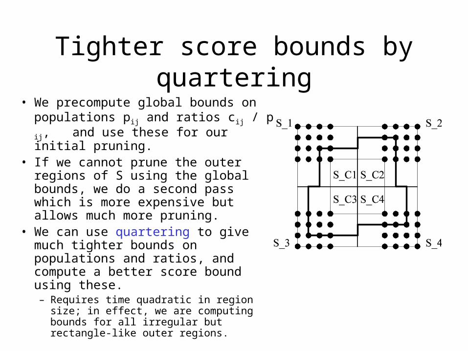
Tighter score bounds by quartering

• We precompute global bounds on populations pij and ratios cij / p ij, and use these for our initial pruning.

• If we cannot prune the outer regions of S using the global bounds, we do a second pass which is more expensive but allows much more pruning.

• We can use quartering to give much tighter bounds on populations and ratios, and compute a better score bound using these.– Requires time quadratic in region size; in

effect, we are computing bounds for all irregular but rectangle-like outer regions.

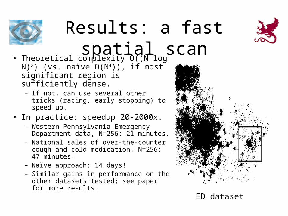
Results: a fast spatial scan• Theoretical complexity O((N log N)2)

(vs. naïve O(N4)), if most significant region is sufficiently dense.– If not, can use several other tricks

(racing, early stopping) to speed up.

• In practice: speedup 20-2000x.– Western Pennsylvania Emergency

Department data, N=256: 21 minutes.– National sales of over-the-counter cough

and cold medication, N=256: 47 minutes.– Naïve approach: 14 days!– Similar gains in performance on the other

datasets tested; see paper for more results.

ED dataset

Results: a fast spatial scan• Potential impact: facilitating fast

disease surveillance by state and local health departments.

• Preliminary results indicate that we can detect elongated regions 10-20x faster than the current state of the art (Kulldorff’s SaTScan software) can detect circular regions.

ED dataset

CAVEAT #1: Inexact comparison!

CAVEAT #2: Comparison to SaTScan is preliminary!

Concluding remarks

• We are currently applying our fast spatial scan algorithm to national-level hospital and pharmacy data, monitoring daily for disease outbreaks.

• We have also extended the algorithm to arbitrary dimension, and applied these techniques to various multidimensional datasets. – For example, we are using the

3D fast spatial scan on fMRI data, in order to discover regions of brain activity corresponding to given cognitive tasks.

In collaboration with the RODS lab at U.Pitt.

In collaboration with Tom Mitchell and Francisco Pereira at CMU.

See our upcoming NIPS paper for more details.