THE 16th CHESAPEAKE SAILING YACHT SYMPOSIUMANNAPOLIS, MARYLAND, MARCH 2003

Numerical Simulation using RANS-based Tools for America’s Cup Design Geoff Cowles, Institut de Mathématiques, Ecole Polytechnique Fédérale de Lausanne, Switzerland Nicola Parolini, Institut de Mathématiques, Ecole Polytechnique Fédérale de Lausanne, Switzerland Mark L. Sawley, Granulair Technologies, Lausanne, Switzerland

ABSTRACT The application of Computational Fluid Dynamics simulations based on the Reynolds Averaged Navier-Stokes (RANS) equations to the design of sailing yachts is becoming more commonplace, particularly for the America's Cup. Drawing on the experience of the Ecole Polytechnique Fédérale de Lausanne as Official Scientific Advisor to the Alinghi Challenge for the America’s Cup 2003, the role of RANS-based codes in the yacht design process is discussed. The strategy for simulating the hydrodynamic flow around the boat appendages is presented. Two different numerical methods for the simulation of wave generation on the water surface are compared. In addition, the aerodynamic flow around different sail configurations is investigated. The benefits to the design process as well as its limitations are discussed. Practical matters, such as manpower and computational requirements, are also considered. NOTATION RANS Reynolds Averaged Navier-Stokes CFD Computational Fluid Dynamics VOF Volume of Fluid PDE Partial Differential Equation IACC International America’s Cup Class

VPP Velocity Prediction Program AWA Apparent Wind Angle TWS True Wind Speed INTRODUCTION

There currently exists a wide range of

Computational Fluid Dynamics (CFD) tools for the numerical simulation of aerodynamic and hydrodynamic flows. Such tools are finding increasing use in a wide range of application areas. For example, in the aerospace and automotive industries, CFD methods have been successfully integrated into the design process. More recently, the introduction of these tools into the marine industry has been motivated in part by their application to racing yacht design (Larsson, 1990; Milgram, 1998). For the America’s Cup and Volvo Ocean races, where syndicate budgets can reach US$100 million, the use of CFD tools is becoming widespread.

A hierarchy of CFD tools exists, characterized by

different levels of validity, complexity, computational cost, ease of use and acceptance within the design community. The least complex methods are based on potential (inviscid and irrotational) flow used in panel codes (Dawson, 1977; Milgram, 1997). These methods can provide valuable information (surface pressure and

global forces) for non-separated flows such as the hydrodynamic flow around boat appendages and the aerodynamic flow around upwind sailing configurations. Since their introduction for America’s Cup design over two decades ago, panel codes have become the basic numerical tool used by design teams. The applicability of such methods can be extended by coupling them with a boundary layer code for the evaluation of a limited range of viscous effects.

More complex viscous flows require the use of more advanced methods such as those based on the resolution of the Reynolds Averaged Navier-Stokes (RANS) equations. Separated flow around the bulb and winglets as well as downwind sailing configurations can be treated with RANS-based tools. Such methods can provide more detailed information about the flow fields leading to increased understanding and hence improved design. The use of these advanced CFD tools, however, requires state–of-the-art software, significant computer resources as well as engineers with specific expertise.

Advanced numerical simulation techniques are becoming more widespread in America’s Cup design as a supplement to the more traditional analysis tools (Caponnetto, 1999; DeBord, 2002). In particular, they are generally used to narrow the field of candidates necessary for expensive experimental testing. This increased usage has been enabled by the continual increase in the performance of both CFD software and computer hardware. The relatively small size of the marine market, however, limits the development of specific yacht design software, its validation and its use by marine engineers. In addition, within the America’s Cup community, the need to maintain a high level of confidentiality of geometries and results renders much of the work unpublished. The intense and periodic nature of the activities surrounding this event limits the time allocated for a systematic long-term application and validation procedure. These factors in turn limit the possibility to increase confidence in the application of advanced CFD tools within the yacht design community. As Official Scientific Advisor to the Alinghi Challenge for the America’s Cup 2003, the Ecole Polytechnique Fédérale de Lausanne (EPFL) has provided scientific research in the areas of fluid dynamics (computational and experimental) and material science (composites and structure testing). In particular, the Institut de Mathématiques has been involved in research activities associated with RANS-based codes. The results obtained were integrated into the design process, together with the results of more traditional numerical tools and experimentation, by the Alinghi design team. The CFD studies performed at the EPFL can be separated into three main areas: hydrodynamic flows (without free surface effects), free surface flows and aerodynamic flows. In the present paper, a specific

description of the analysis procedure is given for each of these areas, providing details of mesh generation, solution procedure and the treatment of boundary conditions. For reasons of confidentiality, only limited numerical results are presented. CFD SIMULATION TOOLS

Two state-of-the-art RANS-based codes were employed for these studies. The particular strengths of each of these codes were utilized for specific studies.

FLUENT 6.0 was used to compute both hydrodynamic and aerodynamic flows around the boat (Fluent, 2001). This commercial software package solves the three-dimensional RANS equations on an unstructured mesh (possibly having mixed element types). The flow solver is based on a finite volume discretization, and provides a choice of numerical methods. The additional availability of a wide variety of physical models enables the use of FLUENT in a large number of application areas. For the present study, mesh generation was undertaken using the FLUENT pre-processor GAMBIT.

An academic code SHIP107MB was also used for hydrodynamic flow studies. This code was developed at Princeton University and modified at the EPFL for application to America’s Cup boats. The code uses a finite volume discretization on a block-structured mesh. The numerical scheme is based on a multi-stage explicit time integration using central differencing and multigrid acceleration. Of specific importance for the present study is the code’s ability to model surface waves by adapting the mesh to track movements of the free surface. Mesh generation for these simulations was performed using the commercial software GRIDGEN (Gridgen, 1999).

Two different types of computer systems were available to perform the different simulation tasks:

• a desktop workstation with two Intel Pentium 4 (1.7 GHz ) processors and 2 GB memory,

• an SGI Origin 3800 central computer system with 128 MIPS R14000 (500 MHz) processors and 64 GB memory.

HYDRODYNAMIC FLOW – APPENDAGES

For the evaluation of appendage configurations the

geometries analyzed were comprised of a hull and a full set of appendages common to IACC racing yachts, including keel, bulb, winglets, and rudder. Due to the complexity of modelling the free surface, as discussed in the next section, a static flat water surface was assumed for the appendage studies, with a symmetry boundary condition placed at the waterplane. The FLUENT code was used for the appendage studies.

A series of studies on winglet shape and placement, bulb shape, and keel shapes were made. In total, approximately 60 different geometric configurations were analyzed. Most of these were evaluated in at least two flow conditions: upwind and downwind. These calculations were used to supply a large variety of information to the Alinghi design team for integration into various stages in the design cycle.

Extensive post-processing efforts were targeted at calculating component forces and visualization of the local fluid flow near specific regions of interest. This information was used to help the designers make shape variations, even in the late stages of appendage component design. Mesh Generation

The most onerous part of the simulation procedure in terms of engineer time and effort is the generation of the computational mesh. In general, this process consists of three major steps:

• CAD geometry cleaning, • surface meshing, • volume meshing.

In the first step, the CAD representation of the

geometry must be rigorously examined to ensure that it meets the constraints of the mesh generation software in terms of surface tolerance and port/starboard symmetry (if applicable). CAD geometries that are unsuitable for CFD analysis (e.g. due to the presence of very small surfaces, gaps and/or overlaps) can be a major bottleneck in the mesh generation process; communication between the engineers performing the CAD design and the mesh generation is critical. Since most mesh generation software has only limited flexibility for the repair and manipulation of the CAD object, streamlining and determination of the optimal settings in the CAD work is crucial.

Flexibility in the mesh topology, as is available in

the FLUENT code, is beneficial and perhaps critical for treating complex geometries such as underwater region of an IACC boat. In general, when using unstructured mixed-element meshes to resolve high-Reynolds-number viscous flow, the surfaces are meshed with triangles/quadrilaterals and layers of prisms/hexahedra are then extruded from the surface to produce a region to capture the boundary shear layer. In the final step, tetrahedrons are generated to fill the remaining volume of the computational domain.

When the surface curvature of critical components,

such as keel and winglet leading edges, is very large, triangulation of the surface will lead to an unmanageable number of elements since the element aspect ratio must remain near unity. For these regions, a quadrilateral surface mesh was used in this work since element aspect

ratios could be increased by an order of magnitude. The short side of the quadrilateral followed the chordwise direction and the long side was placed spanwise. The final surface meshes (see Figure 1) contained around 200,000 elements and utilized a combination of both triangular and quadrilateral elements to provide adequate surface resolution with a mesh of realistic size for an overnight computation.

Fig. 1 Surface mesh of an IACC underbody

After completion of the surface meshing, the volume

containing the shear layer is created. The layer initial spacing, stretching, and thickness of the region are dictated by the Reynolds number, the spatial accuracy of the flow solver, the turbulence model, and the method used to resolve the inner region of the turbulent boundary layer. The algorithm governing the above-mentioned mesh extrusion process is controlled by a large number of parameters that enhance its stability and quality. Determining the combination that results in the desired initial layer spacing, number of layers and total thickness of the region can be very time consuming. In regions of high concavity such as at the winglet/bulb intersection, the growth process often fails and alternate parameters must be chosen.

In the final step of the mesh generation procedure, the external volume is filled with tetrahedrons. In order to temper an excessive growth rate of the tetrahedrons away from the body, a control surface (see Figure 2) was placed around the geometry and triangulated. This surface defined two distinct regions for the tetrahedral mesher to fill and provided a constraint on tetrahedral size at a given distance from the body.

Fig. 2 Outline of heeled geometry and control surface

for tetrahedral meshing

Estimated time requirements to perform the various

steps of the mesh generation process for a generic simulation are indicated in Table 1. The mesh generation was performed using the desktop workstation. In total, the entire mesh generation process required around 2 to 6 hours per mesh. This was highly dependent on the quality of the initial CAD geometry. Table 1 indicates that due to recent advances in mesh generation software, a complex geometry can now be meshed with relatively modest engineer and computer time and resources.

Mesh Generation Step Engineer time

Computational time

Geometry repair 15 min - 3 hr 5 min

Surface meshing 40 min 5 min

Shear layer extrusion 15 min - 1 hr 15 min

Tetrahedral meshing 20 min 15 min

TOTAL 1.5 hr - 5 hr 40 min

Table 1 Estimates of mesh generation time requirements

Physical Modelling

The chord or length based Reynolds numbers of all the underbody elements of an IACC racer allows substantial regions of laminarity. Use of a fully turbulent assumption will lead to inaccurate estimates of the frictional as well as the pressure drag. FLUENT includes a large variety of turbulence models, however, none of them incorporated a mechanism for the simulation of transition. This problem may be circumvented by marking certain regions of the mesh as “laminar” which forces the flow solver to suppress the evolution of the eddy viscosity (turbulence) in this region (see Figure 3). However, gaining the necessary information to define the extent and location of these zones is a difficult task. It can be

obtained through experimental work (Lurie, 2001) or by using a panel method coupled with an integral boundary layer code containing a dependable transition model such as an eN type (Drela, 1989). Both methods were used by the Alinghi design team to provide estimates of the transition line locations on the various appendages.

Fig. 3 Keel and bulb surfaces showing typical zones for

laminar treatment (red)

Cases Run

In general, two types of cases were run for the hydrodynamic studies: downwind and upwind. For the downwind cases, the included geometry consisted of the hull, keel, and winglets. The flow was port/starboard symmetrical for these cases, but for simplicity the complete mesh was constructed. For the upwind cases, the rudder was included and the tab was deflected and the geometry was heeled and yawed.

The mesh sizes and computational times are

indicated in Table 2. The computational times are quoted for 16 processors of the SGI Origin 3800 computer system.

Configuration Downwind Upwind

Geometry Hull/Keel/Wlets Hull/Keel/Wlets/Rudder

Surface mesh 180,000 faces 200,000 faces

Volume mesh 4,500,000 elements 5,500,000 elements

Runtime 8 hr 10 hr

Table 2 Mesh sizes and computational times

Post-Processing A primary benefit of RANS-based tools for the

hydrodynamic studies derives from the wealth of information that may be deduced during the post-processing phase. Panel methods are able to only provide surface pressure distributions and global metrics such as lift and drag. Methods that calculate forces using a Trefftz-plane cut are not even able to resolve forces by component. This limited amount of information makes it difficult for the designers and fluid dynamicists to decipher the causes behind any differences in performances calculated for various configurations.

By exploring the RANS solution with a good

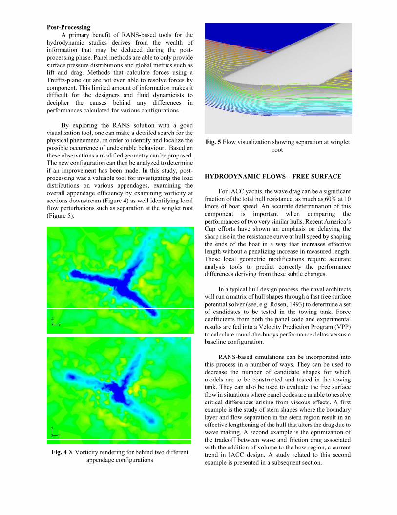
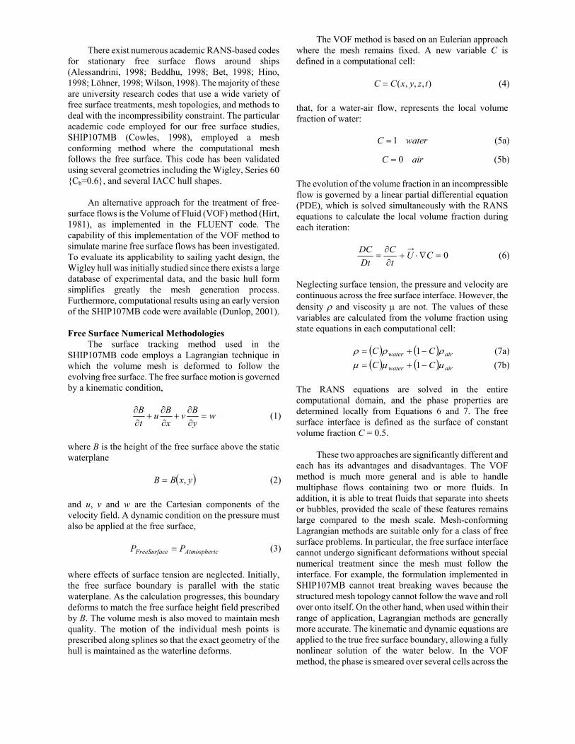
visualization tool, one can make a detailed search for the physical phenomena, in order to identify and localize the possible occurrence of undesirable behaviour. Based on these observations a modified geometry can be proposed. The new configuration can then be analyzed to determine if an improvement has been made. In this study, post-processing was a valuable tool for investigating the load distributions on various appendages, examining the overall appendage efficiency by examining vorticity at sections downstream (Figure 4) as well identifying local flow perturbations such as separation at the winglet root (Figure 5).

Fig. 4 X Vorticity rendering for behind two different

appendage configurations

Fig. 5 Flow visualization showing separation at winglet

root

HYDRODYNAMIC FLOWS – FREE SURFACE

For IACC yachts, the wave drag can be a significant

fraction of the total hull resistance, as much as 60% at 10 knots of boat speed. An accurate determination of this component is important when comparing the performances of two very similar hulls. Recent America’s Cup efforts have shown an emphasis on delaying the sharp rise in the resistance curve at hull speed by shaping the ends of the boat in a way that increases effective length without a penalizing increase in measured length. These local geometric modifications require accurate analysis tools to predict correctly the performance differences deriving from these subtle changes.

In a typical hull design process, the naval architects

will run a matrix of hull shapes through a fast free surface potential solver (see, e.g. Rosen, 1993) to determine a set of candidates to be tested in the towing tank. Force coefficients from both the panel code and experimental results are fed into a Velocity Prediction Program (VPP) to calculate round-the-buoys performance deltas versus a baseline configuration.

RANS-based simulations can be incorporated into

this process in a number of ways. They can be used to decrease the number of candidate shapes for which models are to be constructed and tested in the towing tank. They can also be used to evaluate the free surface flow in situations where panel codes are unable to resolve critical differences arising from viscous effects. A first example is the study of stern shapes where the boundary layer and flow separation in the stern region result in an effective lengthening of the hull that alters the drag due to wave making. A second example is the optimization of the tradeoff between wave and friction drag associated with the addition of volume to the bow region, a current trend in IACC design. A study related to this second example is presented in a subsequent section.

There exist numerous academic RANS-based codes

for stationary free surface flows around ships (Alessandrini, 1998; Beddhu, 1998; Bet, 1998; Hino, 1998; Löhner, 1998; Wilson, 1998). The majority of these are university research codes that use a wide variety of free surface treatments, mesh topologies, and methods to deal with the incompressibility constraint. The particular academic code employed for our free surface studies, SHIP107MB (Cowles, 1998), employed a mesh conforming method where the computational mesh follows the free surface. This code has been validated using several geometries including the Wigley, Series 60 {Cb=0.6}, and several IACC hull shapes.

An alternative approach for the treatment of free-

surface flows is the Volume of Fluid (VOF) method (Hirt, 1981), as implemented in the FLUENT code. The capability of this implementation of the VOF method to simulate marine free surface flows has been investigated. To evaluate its applicability to sailing yacht design, the Wigley hull was initially studied since there exists a large database of experimental data, and the basic hull form simplifies greatly the mesh generation process. Furthermore, computational results using an early version of the SHIP107MB code were available (Dunlop, 2001). Free Surface Numerical Methodologies

The surface tracking method used in the SHIP107MB code employs a Lagrangian technique in which the volume mesh is deformed to follow the evolving free surface. The free surface motion is governed by a kinematic condition,

wyΒv

xΒu

tΒ

=∂∂

+∂∂

+∂∂ (1)

where B is the height of the free surface above the static waterplane (2) ( yxΒΒ ,= )

and u, v and w are the Cartesian components of the velocity field. A dynamic condition on the pressure must also be applied at the free surface, (3) cAtmospherieFreeSurfac PP =

where effects of surface tension are neglected. Initially, the free surface boundary is parallel with the static waterplane. As the calculation progresses, this boundary deforms to match the free surface height field prescribed by B. The volume mesh is also moved to maintain mesh quality. The motion of the individual mesh points is prescribed along splines so that the exact geometry of the hull is maintained as the waterline deforms.

The VOF method is based on an Eulerian approach where the mesh remains fixed. A new variable C is defined in a computational cell: ),,,( tzyxCC = (4) that, for a water-air flow, represents the local volume fraction of water: waterC 1= (5a)

airC 0= (5b)

The evolution of the volume fraction in an incompressible flow is governed by a linear partial differential equation (PDE), which is solved simultaneously with the RANS equations to calculate the local volume fraction during each iteration:

0=∇⋅+∂∂

= CUtC

DtDC (6)

Neglecting surface tension, the pressure and velocity are continuous across the free surface interface. However, the density ρ and viscosity µ are not. The values of these variables are calculated from the volume fraction using state equations in each computational cell: ( ) ( ) airwater CC ρρρ −+= 1 (7a) ( ) ( ) airwater CC µµµ −+= 1 (7b) The RANS equations are solved in the entire computational domain, and the phase properties are determined locally from Equations 6 and 7. The free surface interface is defined as the surface of constant volume fraction C = 0.5.

These two approaches are significantly different and each has its advantages and disadvantages. The VOF method is much more general and is able to handle multiphase flows containing two or more fluids. In addition, it is able to treat fluids that separate into sheets or bubbles, provided the scale of these features remains large compared to the mesh scale. Mesh-conforming Lagrangian methods are suitable only for a class of free surface problems. In particular, the free surface interface cannot undergo significant deformations without special numerical treatment since the mesh must follow the interface. For example, the formulation implemented in SHIP107MB cannot treat breaking waves because the structured mesh topology cannot follow the wave and roll over onto itself. On the other hand, when used within their range of application, Lagrangian methods are generally more accurate. The kinematic and dynamic equations are applied to the true free surface boundary, allowing a fully nonlinear solution of the water below. In the VOF method, the phase is smeared over several cells across the

interface and substantial regions will exist having properties (density and viscosity) that are intermediate between water and air (see Figure 6). The interface smearing is a result of the spatial discretization of the phase equation and thus the solution becomes dependent on the density of the mesh near the interface. The accuracy of the VOF method also suffers from mesh sensitivity. Clustering the mesh near the free surface will improve the crispness of the phase boundary. However, since the location of the free surface is not known a priori, one usually takes the approach of clustering the mesh lines towards the static waterplane during the mesh generation process. For large free surface deformations at high Froude number, the calculated free surface may be far from the high-density mesh region.

Fig. 6 Phase distribution on the Wigley hull showing dissipation of the interface: air (red) and water (blue)

Wigley Hull Calculations

The Wigley hull forms are described analytically by a quadratic equation. The transverse (beam) coordinate is expressed as a function of the longitudinal (x) and vertical (z) coordinates

−

−=

22

1212 D

zLxby (8)

where b is the beam, D is the draft and L is the hull length. For the present study, the hull specification parameters were chosen to be b/L = 1/10, D/L = 1/16. This particular Wigley hull is commonly used for code validation, since experimental data is available from several datasets. For this study, the University of Tokyo contribution to the 1983 Wigley Cooperative Study was used (ITTC, 1983). In these experiments, resistance data as well as waterline profiles were obtained from a towed 2.5 m model over a large range of Froude numbers (0.1 - 0.408).

The mesh used for testing the VOF calculations using FLUENT is shown in Figure 7. It is a single-block structured mesh consisting of 230 longitudinal, 50 transverse and 100 vertical mesh points, with 150

longitudinal and 70 vertical points on the hull surface. The computational domain is a box situated at –6.25 m < x < 3.75 m, 0 m < y < 5 m, -2 m < z < 0.3 m. The hull is centered at the origin and is 2.5 m in length. Since for the VOF method both the air and water regions must be modelled, the Wigley hull was extended vertically upward 0.3 m to give it a rather large false freeboard. The vertical extent of the air zone should be large enough so that the presence of the upper far field boundary will not perturb the resulting solution. Two zones of mesh clustering are discernable in Figure 7, the high-density regions forming the shear layer and the initial fluid interface at the static waterplane. The first region is necessary in any RANS calculation to capture the velocity gradient near the hull. The second clustering is necessary in volume tracking methods for an accurate resolution of the free surface. The mesh is clustered in the vicinity of the static waterplane with a minimum vertical mesh spacing of 3 mm. A single-block structured mesh was also used for the simulations using the SHIP107MB code. The dimensions of the mesh were 289 longitudinal, 65 transversal and 49 vertical mesh points. The computational domain stretched 1.5 boat lengths before the boat and 2.5 boat lengths aft, to starboard and below.

Fig. 7 Wigley hull mesh used for the VOF simulation

The computation using FLUENT required 30 hours

on 16 processors of the SGI Origin 3800. The SHIP107MB calculation required 1.5 hours on 9 processors of an IBM SP2 (which for this code is estimated to have half the computational speed of the Origin 3800). This substantial difference in computation time is attributed to the significantly faster convergence of the flow solver as well as the free surface method used in the SHIP107MB code.

Comparisons of the resulting overhead wave elevations are shown in Figure 8. The wave patterns obtained by the two codes are in good agreement.

Fig. 8 Free surface elevation comparison, Fr=0.25: FLUENT (top), SHIP107MB (bottom)

The specific behaviour of the two methods can be

better understood analyzing waterline profiles calculated using the two codes and data taken from experiment (as shown in Figures 9 and 10). The bow wave amplitude appears to be better determined by the VOF method. On the other hand, the diffusion of the interface (Figure 6) leads to a loss of accuracy in the wave profile downstream along the hull, confirming the comments of the previous section. The measurement error in determining the experimental profiles is not provided in the towing tank report. However, error in the acquisition of this data is generally on the order of 2 mm, which is about 6% percent of the magnitude of the bow wave in the low Froude case and 3% percent in the high Froude case.

Fig. 9 Wave Profile comparison, Wigley hull (Fr =

0.25)

Fig. 10 Wave Profile comparison, Wigley hull (Fr

=.408)

Values for the frictional and pressure resistance and comparison with experiment are displayed in Table 3. The force calculated by SHIP107MB is consistently 2% high while the forces calculated using FLUENT are within 1% of the experimental value as shown in Table 4. Froude No. Ct - FLUENT Ct - SHIP107MB Ct – Expt

0.250 4.593 4.681 4.612

0.408 5.748 5.833 5.719

Table 3 Comparison of the total resistance coefficients (x 1000) for the Wigley hull

Froude No. Ct - FLUENT Ct - SHIP107MB

0.250 0.403 1.496

0.408 0.499 1.993

Table 4 Total resistance error comparison (%) for the Wigley hull

America’s Cup Class

There exist several important differences between the Wigley hull described above and an IACC hull. In particular, the Wigley hull has very fine waterline entrance and exit angles, vertical sides, and a small beam/length ratio. An IACC hull has much more volume forward, a much larger overhang (flare) along most of the hull, and a larger beam to length ratio. These shape differences give rise to three additional challenging aspects for free surface simulation. The larger beam to length ratio produces stronger linearities in the near field wave elevation. The large entry angle and increased volume forward in the IACC hulls gives rise to spilling bow waves observed in the upper range of their racing speeds (9-13 knots). Finally, the gently sloping aft buttock lines of the IACC hull makes the prediction of the location and pattern of flow separation from the hull more difficult to calculate accurately.

Using the experience gained from the work using

FLUENT for the Wigley hull, a mesh was constructed for the IACC hull. The very shallow angle of the hull at the forward and aft perpendiculars of the profile caused some difficulty in the construction of the mesh since the high density regions in the boundary layer and around the static waterplane were nearly parallel at their points of intersection. This lead to highly skewed elements near the bow and stern. Initial tests were made in which a symmetry plane condition was applied to the static waterplane to eliminate any interaction between the air and water fluids. This solution converged quickly and the resulting viscous drag on the hydrodynamic elements compared well with estimates determined from the ITTC friction line. When the symmetry plane condition was removed and the free surface was free to evolve, however, the resulting solution for the free surface field was completely unphysical. Numerous attempts to determine the source of the difficulties and to improve the situation were made, including an expansion of the computational domain to reduce reflections during calculation, adjustment of the coefficients controlling the computation, and the creation of a number of alternate mesh topologies. Unfortunately, no realistic solution has been obtained to date.

The wave resistance calculation of IACC hulls has

therefore been undertaken solely using the SHIP107MB code. To do so, however, some modifications were required to the free surface algorithm. Since the Lagrangian free surface treatment could not simulate the spilling fluid at the bow, wave breaking had to be numerically suppressed. Two strategies exist to achieve this goal:

• augment the energy balance through alteration of the dynamic free surface boundary condition (Equation 3) to mimic dissipation in the breaking wave,

• geometrically reconstruct the shape of the free surface in order to eliminate the multi-valued functional regions.

The first method has been used successfully for two-

dimensional flows (Subramani 1998). Regions of potential wave breaking were detected using a metric that was based on free surface curvature. A damping term was then added locally to the dynamic boundary condition, in effect removing energy from the system. An attempt was made in the present study to extend this method to three dimensions, but it was difficult to construct a robust scheme that was not heavily dependent on somewhat arbitrary parameters. A similar finding has been reported by other workers (Alessandrini, 1998).

The second strategy, based on geometric

suppression, was therefore employed. Such a strategy has also been previously applied to two-dimensional flows by Subramani, 2000. When the wave surface is too sharp

according to some criteria, the mesh points forming the cusp are temporarily removed from the system and a cubic spline fit through the remaining points in the vicinity of the cusp, producing a smooth surface. With a block-structured method, such as used in SHIP107MB, point removal is not viable. However, local smoothing of the free surface is possible. The basic strategy is to incorporate a smoothing of the free surface height field that is active in the regions of high curvature and robustly smooth the discontinuities in the surface field. An algorithm based on the Local Extremum Diminishing (LED) class of methods was implemented for this purpose (Jameson, 1995). This describes a class of numerical stabilization algorithms that have been successfully utilized for the computation of transonic flows where discontinuities exist in the form of shock waves. For the present application, the discontinuities are breaking waves. When the mesh begins to cusp, the limiters become active and the mesh is held in position. This represents a linearization of the free surface about a deformed state. The accuracy of this local linearization can only be determined by comparison of the computed results with experimental data.

For the calculation of flow around the IACC hull using SHIP107MB, an O-type mesh was used. The dimensions of the mesh were 193x65x49 points in the longitudinal, transversal (shear layer) and vertical directions. The resolution on the hull was 193x49 points. Resistance evaluations of a bare hull at zero heel and yaw angles were made for a range of Froude numbers at model-scale (λ = 1/3) Reynolds numbers. Sink and trim conditions were prescribed by the Alinghi design team. The calculations required 6 hours on six processors of the SGI Origin 3800.

Comparison of computed resistance values (in

relative units) with experimental data from a towing tank is shown in Figure 11. The percentage differences between the calculated results and experimental data are shown in Table 5.

0.0

0.2

0.4

0.6

0.8

1.0

6.5 7 7.5 8 8.5 9 9.5 10 10.5 11

boat speed [kn]

pressure (comp.)

friction (comp.)

total (comp.)

total (exp.)

Fig. 11 Total resistance comparison, IACC boat (model

scale)

The good agreement obtained provides an indication that the numerical suppression of wave breaking as implemented was not detrimental to the accuracy of the calculation. The improvement over the results on the Wigley hull shown in the previous subsection can be attributed to two years of further development and validation. After assessing the accuracy of the SHIP107MB code in the computation of IACC hull resistance, it was utilized in a specific bow shape study to help determine the range of boat speed for which an increase in forward volume is beneficial.

Boat Speed 7 kn 8 kn 8.5 kn 9 kn 9.5 kn 10 kn

Error (%) 1.61 -0.22 -1.13 -1.67 -0.89 0.12

Table 5 Relative error in the resistance calculation, IACC boat

AERODYNAMIC FLOWS

The determination of aerodynamic flows for racing yachts is complicated by the fact that sails are not rigid and the prediction of their true flying shape requires the determination of equilibrium between material and fluid mechanical loadings. In addition, the inflow conditions are complicated by the presence of a vertical wind shear, the nature of which is dependent on sea state and other factors. While specialized wind tunnels for scale model testing of sails have been constructed, most sail development programs rely solely on the experience of sail designers and sailors, as well as full-scale two-boat testing, for the determination of optimal sail shapes.

The use of advanced computational tools for sail design is slowly progressing. The sensitivity of computational results and numerical (e.g. mesh, time step) and physical (turbulence) modelling, combined with a lack of suitable experimental data make it difficult to undertake a detailed study of the accuracy of the various methods. Computational simulation of aerodynamic forces on sails can be separated into two categories: upwind and downwind. The different flow conditions for these two points of sail can influence the appropriate choice of numerical simulation tool. In most studies, the sails are treated as inextensible surfaces that are pre-positioned in their theoretical or measured flying shape. Empirical relations for the atmospheric boundary layer are commonly used to prescribe the vertical wind shear at the inflow boundary.

In upwind sailing, the flow generally remains

attached over the vast majority of the sail surface with the exception of a small region aft of the mainsail luff. This region of laminar separation is caused by the presence of the mast, which cannot be mechanically rotated to a more aerodynamic position according to the IACC design rules

(IACC, 2000). For upwind sails, the aero-elastic coupling of the sails can be numerically simulated using a coupled flow-structure approach, as employed by the Flow/Membrain code of North Sails Inc. Such an approach can provide estimates of the sail force coefficients on the resulting flying shape (Caponnetto, 1998). A rapid evaluation of a number of sail shapes can be undertaken, and the information easily incorporated into the VPP. However, a potential flow solver (such as Flow) is not able to simulate or capture the region of separation aft of the mast. This leads to errors in the calculation of the side force and driving force, resulting in the need for empirical correlations to correct the results. Numerical simulations of upwind sail shapes using RANS-based codes, such as FLUENT, have been shown to be able to predict accurately the level and extent of the separated region aft of the mast (Caponnetto, 1998; Wynne, 2002).

In downwind sailing, there are significant regions of

separation on the main and spinnaker resulting from the large angle of attack. Downwind sail shapes remain a critical element in the search for speed gains in the America’s Cup. The significant regions of separated and unsteady flow necessitate, in principle, the use of computationally intense, time-accurate viscous flow solvers for numerical simulation. Nevertheless, some successful efforts have indicated the utility of RANS-based methods for downwind sail configurations (Sawley, 1998).

The present study concentrated on the numerical simulation of the flow around downwind sailing configurations. Three specific aspects of downwind sailing aerodynamic simulation have been considered: calculation of forces, two-boat interaction, and the evolution of the wind shadow. Downwind Sail Forces

The FLUENT code was also used for the downwind aerodynamic simulations. The geometries used include the exposed hull, mainsail, symmetrical spinnaker, and appendages. Appropriate values of the flow conditions (sailing angle, true wind speed and hull speed) were prescribed.

For these cases, both the hydrodynamic and

aerodynamic regions were modelled. The two fluid regions (air and water) were prevented from interacting by the presence of a symmetry boundary condition at the static waterplane. The primary purpose of including the hydrodynamic component was to provide a first approximation for solving the fully-coupled aero-hydrodynamic system. With the addition of both a free surface and a dynamic motion of the geometry in response to the forces in an iterative process, it should be possible to construct a simplified VPP based on the RANS equations.

The extent of the computational domain for the

calculations was 300 m in the direction of hull travel, 200 m in the transverse direction, and 180 m vertically. The relative size of the bounding box and location of the geometry inside can be seen in the graphical representation in Figure 12.

Fig. 12 Computational domain for downwind sailing

simulation

Since the intention of the present study was to

provide an initial investigation of numerical simulation of downwind configurations, the computational mesh was designed to provide the essential flow characteristics without necessarily trying to capture all the fine details. The surface mesh (for both the aerodynamic and hydrodynamic regions) was comprised of a total of 370,000 triangular elements, part of which is depicted in Figure 13. The volume mesh contained 2,050,000 tetrahedral elements. These mesh size parameters were based on previous validation studies that had resulted in good agreement with experiment (Sawley, 1998). Due to the already sizeable number of mesh cells for this mesh, structured (prismatic) boundary layer meshes were not added near the boat or water surfaces.

Fig. 13 Surface mesh used for downwind simulations

A boat speed of 10 knots, true wind speed of 15 knots and true wind angle was 160° was considered. The relatively small mesh size for this case enabled computation on the desktop dual-processor workstation, and required around 12 hours.

Figure 14 shows an aerial view of the streamlines around the spinnaker. Figure 15 displays the pressure contours on both the windward and leeward sides of the sail surfaces. The flow appears to be attached over the major part of the leeward surface of the spinnaker. This is not surprising given that the apparent wind angle (AWA) is significantly less than 180o. However, due to the relatively coarse mesh used for this simulation, it is to be expected that any strong boundary layer effects – such as flow separation off curved surfaces – were not accurately simulated. Based on an analysis of the driving and side forces, as well as an examination of the region of separation (Figures 14 and 15), the sails appear to act as a combination of a parachute (with the lift aligned with the direct of thrust) and a vertical wing (drag aligned with the direction of thrust), as concluded by Richards, 2001.

Fig. 14 Flow streamlines around the symmetrical

spinnaker

Blanketing The physics underlying the tactical advantage of the

safe leeward position in upwind sailing are well understood and are often treated in textbooks on sail trim and tactical sailing (Whidden, 1990). Downwind match racing tactics are dominated by downwind covering, or “blanketing”, which is governed by more complex fluid dynamics. The large-scale regions of complex vortical flow leaving the windward yacht interact with the wind gradient and manifest themselves in a perturbation of the freestream conditions, which can adversely affect the progress of the leeward yacht. This perturbation is known as the “wind shadow”.

Fig. 15 Surface pressure on the windward (top) and

leeward (bottom) sail surfaces

Two types of simulations were carried out to better

understand blanketing. In the first study, two boats sailing in a downwind coverage situation were simulated to examine the interaction between them. In the second study, a detailed flow solution of a single yacht on a downwind leg was performed to provide quantitative and qualitative information about the evolution of the wind shadow. Information of this kind can support the tactical decisions of both the leading and trailing yachts to maximize coverage or minimize its damaging effects.

Two-Boat Simulations This study provides a detailed view of the interaction

between two boats through aerodynamic shadowing. Rather than examine the properties of the wind shadow and indirectly deduce its potential influence on another boat, the addition of a second boat in the simulation allows this influence to be directly determined. By choosing two identical boats, the influence of the different flow fields experienced by each boat can therefore be assessed.

In reality the boats will have their sails trimmed

differently to the different wind conditions. In the absence

of fluid-structure effects in the simulation, this more detailed interaction cannot be accounted for.

A graphical depiction of the computational domain is shown in Figure 16. For this simulation, the bounding box was 300x200x130 meters in the x, y and z directions accordingly. As in the single boat simulation described in the previous section, the hydrodynamic portion of the domain was also meshed. Since the aerodynamic and hydrodynamic flows are again uncoupled in this study, the inclusion of the latter is not necessary for an analysis of aerodynamic phenomena. The total volume mesh was comprised of 4,600,000 tetrahedral cells. The sailing conditions were prescribed by a boat speed of 10 knots, a true wind speed of 15 knots and a true wind angle of 165°. To simplify the calculation, no wind gradient was prescribed at the inflow boundary. The boats were separated by 1.8 boat lengths and the trailing boat was located 141° to windward of the leader. The calculation required about 12 hours on 8 processors of the SGI Origin 3800 computer system.

Fig. 16 Plan view of computational domain for the two-

boat simulation

Figure 17 shows an aerial view of the positioning of

the boat in the wind shadow. Clearly the wind speed and angle varies greatly over the full extent of the sails. This results in a significant change in the aerodynamic forces exerted on the leeward boat’s sails. A visual indication of this change is shown in Figure 18. The pressure on the windward surface of the two boats’ sails is observed to be substantially different both in magnitude and in spatial distribution leading to a significant difference in the driving forces of the two configurations. Some of this difference would normally be compensated by an alteration of the sail trim of the leeward boat.

Fig. 17 Streamlines indicating the perturbation of the

freestream conditions of the leeward boat

Fig. 18 Surface pressure on two boats in a downwind

coverage scenario

Wind Shadowing In order to obtain a more qualitative and quantitative

assessment of the wind shadow, this study employed more realistic sail geometries and flow conditions, incorporated the atmospheric boundary layer, and used a larger computational domain. With respect to the aerodynamic study discussed above, the computational bounding box was enlarged considerably to 500x400x160 m in the x, y and z directions respectively. A symmetry plane was placed at z = 0, with no meshing or modelling of the hydrodynamic flow. The geometry included the same hull, mainsail and symmetrical spinnaker and was discretized by 490,000 triangular elements. The final volume mesh contained 3,169,000 tetrahedral cells. An atmospheric boundary condition was applied at the inflow. Because the hull was stationary in the simulation, the variation in both the magnitude of the apparent wind and the apparent wind angle (AWA) was prescribed. This was derived from the boat speed, sailing angle, and a relation for the true wind

speed obtained from an approximation of the atmospheric boundary layer. For this study, the 1/10 law was used to model the true wind speed (TWS) in this layer,

[ ] 1.010)10()( zTWSzTWS ⋅= (9)

where z is the vertical coordinate in meters measured from the static waterplane. The computations required 12 hours using 8 processors of the SGI Origin 3800.

A qualitative assessment of the simulation results reveals the flow to be dominated by the two trailing vortices generated at the head and base of the spinnaker and mainsail (Figure 19). These vortices extend many boat lengths and can provide a significant influence on the aerodynamic forces exerted on the downwind boat. The sail heads produce the largest wind shadow, presumably due to the more localized origin and the weaker influence of the water surface. The angle of propagation of these vortices is observed to be different. The vortex from the sail head appears to propagate at an angle close to the AWA, but is displaced about a boat length upstream. This displacement is presumably due to the strong geometric curvature of the spinnaker, which has the effect of diverting the flow towards the stern.

Fig. 19 Trailing vortices generated at the head and base

of the downwind sails

The presence of the boundary layer complicates

somewhat the quantitative analysis of the flow since, even in the absence of the boat, velocity gradients exist. To obtain the influence of the boat, and hence the shadowing effects, it is necessary to subtract the unperturbed fields to obtain the defect quantities. We define the defect velocity as the magnitude of the difference between the local velocity and the imposed inflow boundary velocity (Vbcx, Vbcy).

( ) ( )[ ] 5.0222zbcyybcxxdefect VVVVVV +−+−= (10)

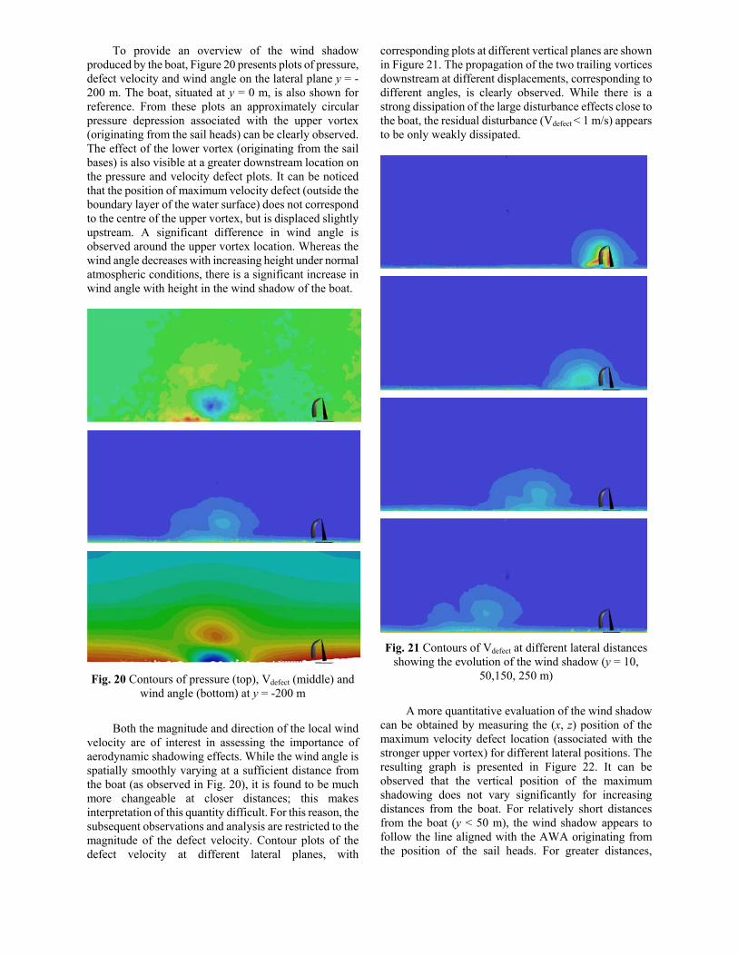
To provide an overview of the wind shadow produced by the boat, Figure 20 presents plots of pressure, defect velocity and wind angle on the lateral plane y = -200 m. The boat, situated at y = 0 m, is also shown for reference. From these plots an approximately circular pressure depression associated with the upper vortex (originating from the sail heads) can be clearly observed. The effect of the lower vortex (originating from the sail bases) is also visible at a greater downstream location on the pressure and velocity defect plots. It can be noticed that the position of maximum velocity defect (outside the boundary layer of the water surface) does not correspond to the centre of the upper vortex, but is displaced slightly upstream. A significant difference in wind angle is observed around the upper vortex location. Whereas the wind angle decreases with increasing height under normal atmospheric conditions, there is a significant increase in wind angle with height in the wind shadow of the boat.

Fig. 20 Contours of pressure (top), Vdefect (middle) and

wind angle (bottom) at y = -200 m

Both the magnitude and direction of the local wind

velocity are of interest in assessing the importance of aerodynamic shadowing effects. While the wind angle is spatially smoothly varying at a sufficient distance from the boat (as observed in Fig. 20), it is found to be much more changeable at closer distances; this makes interpretation of this quantity difficult. For this reason, the subsequent observations and analysis are restricted to the magnitude of the defect velocity. Contour plots of the defect velocity at different lateral planes, with

corresponding plots at different vertical planes are shown in Figure 21. The propagation of the two trailing vortices downstream at different displacements, corresponding to different angles, is clearly observed. While there is a strong dissipation of the large disturbance effects close to the boat, the residual disturbance (Vdefect < 1 m/s) appears to be only weakly dissipated.

Fig. 21 Contours of Vdefect at different lateral distances

showing the evolution of the wind shadow (y = 10, 50,150, 250 m)

A more quantitative evaluation of the wind shadow

can be obtained by measuring the (x, z) position of the maximum velocity defect location (associated with the stronger upper vortex) for different lateral positions. The resulting graph is presented in Figure 22. It can be observed that the vertical position of the maximum shadowing does not vary significantly for increasing distances from the boat. For relatively short distances from the boat (y < 50 m), the wind shadow appears to follow the line aligned with the AWA originating from the position of the sail heads. For greater distances,

however, the wind shadow maximum appears further upstream.

0 50 100 150 200 250 300

lateral position [m]

disp

lace

men

t [m

]x position

z position

Fig. 22 Streamwise and vertical displacement of the

wind shadow

CONCLUSION

Numerical simulations based on the Reynolds Averaged Navier-Stokes equations have provided an array of qualitative and quantitative assessments in support of the Alinghi Challenge for the America’s Cup 2003. Computations have been made using both commercial and academic codes. The applications were divided into three groups (appendage, free surface, and aerodynamic), and ranged from appendage force calculations to a study of the wind shadow.

The hydrodynamic appendage studies were preceded by an intense effort to produce high-quality mixed-element meshes for accurate resolution of the frictional and pressure forces. Post-processing of these simulation results also provided load distributions and lead to a better understanding of the flow physics through visualization. This information was utilized for the explanation of performance differences between configurations. It was also used to determine how an appendage shape should be modified for improvement.

For the free surface studies, tests of the VOF method to predict boat resistance in free surface flows were made. The resistance values obtained compare well with experimental results for the Wigley hull. Additional studies are required, however, to obtain viable results for the more realistic case of an IACC hull. Calculations of the free surface flow around an IACC hull using the mesh conforming method implemented in the SHIP107MB code written proved to be more reliable. Results from these calculations have been used for a detailed study of IACC bow shapes.

The aerodynamics studies undertaken indicate that advanced numerical simulation can provide both a qualitative and quantitative assessment of the aerodynamic flow around a sailing boat. In particular, an initial investigation of the aerodynamic shadowing due to

an IACC boat was undertaken by examining the behaviour of the trailing vortices and the change in the flow velocity downwind of the sails. Information obtained from such simulations can be useful for making tactical decisions regarding boat positioning on downwind legs.

This paper provides examples of how RANS-based simulations may be useful in the design process, as well as the time and manpower required to run them. Nevertheless, much work remains to be performed to improve the level of confidence of RANS-based codes within the yacht design community. This is crucial for the role of these tools in the design cycle to increase and the range of applications to diversify. ACKNOWLEGEMENTS

The authors wish to acknowledge the Alinghi design team for their support in explaining the intricacies of an IACC racing yacht. Their patience in divulging various aspects of the design procedure was greatly appreciated. Also acknowledged is the interest and support of Prof. Alfio Quarteroni (IMA–EPFL), who was willing to add this research area to his group’s existing activities. We would also like to thank Prof. Luigi Martinelli (Princeton University) for his assistance in implementing a robust algorithm for the numerical suppression of breaking waves in the SHIP107MB code. REFERENCES Alessandrini, B. and Delhommeau, G., “Viscous Free Surface Flow Past a Ship in Drift and Rotating Motion,” 22nd Symposium on Naval Hydrodynamics, Washington 1998. Beddhu, M., Nichols, S., Jiang, M.Y., Sheng, C., Whitfield, D.L., and Taylor, L.K., “Comparison of EFD and CFD Results of the Free Surface Flow Field about the Series 60 Cb=.6 Ship,” 25th American Towing Conference, Iowa City, IA, 1998. Bet, F., Hänel, D., and Sharma, S., “Numerical Simulation of Ship Flow by a Method of Artificial Compressibility,” 22nd Symposium on Naval Hydrodynamics, Washington, 1998. Caponnetto, M., Castelli, A., Bonjour, B., Mathey, P.-L., Sanchi, S., and Sawley, M.L., “America’s Cup Yacht Design Using Advanced Numerical Flow Simulations, EPFL Supercomputing Review, 10 (1998) 24-28. Caponnetto, M., Castelli, A., Dupont, P., Bonjour, B., Mathey, P.-L., Sanchi, S., and Sawley, M.L, “Sailing Yacht Design using Advanced Numerical Flow Simulations,” 14th Chesapeake Sailing Yacht Symposium, Annapolis, MD, 1999.

Cowles, G. and Martinelli, L., “A Viscous Multiblock Flow Solver for Free Surface Calculations on Complex Geometries,” 22nd International Symposium on Naval Hydrodynamics, Washington, DC, 1998 Dawson, C.W., ”A Practical Computer Method for Solving Ship-Wave Problems,” 2nd Int. Conf. Numerical Ship Hydrodynamics, Berkeley, CA, 1977. DeBord, F., Jr., Reichel, J., Rosen, B. S., Fassardi, C., “Design Optimization for the International America’s Cup Class”, SNAME Annual Meeting, Boston, MA, 2002. Drela, M., “XFOIL: An Analysis and Design System for Low Reynolds Number Aerodynamics,” Conference on Low Reynolds Number Aerodynamics, Notre Dame University, 1989. Dunlop, M, “Analysis of a Sailboat Hull using Computational Fluid Dynamics”, Semester Project, Department of Mechanical and Aerospace Engineering, Princeton University, 2001. Fluent 6 User’s Guide, Fluent Inc (2001); www.fluent.com. Gridgen User Manual (Version 13.3), Pointwise Inc. (1999); www.pointwise.com. Hirt, C.W and Nichols, B.D., “Volume of Fluid (VOF) Method for the Dynamics of Free Boundaries”. Journal of Computational Physics 1981; 39:201-225. Hino, T., “Navier-Stokes Computations of Ship Flows on Unstructured Grid,” 22nd Symposium on Naval Hydrodynamics, Washington, 1998. IACC, “America’s Cup Class Rule, Version 4.0,” Challenger of Record and Defender for America’s Cup XXXI, October 2000. ITTC Resistance Committee, “Cooperative Experiments on Wigley Parabolic Models in Japan.” 17th ITTC Resistance Committee Report, 2nd ed., 1983. Jameson, A., "Analysis and Design of Numerical Schemes for Gas Dynamics 1, Artificial Diffusion, Upwind Biasing, Limiters, and their Effects on Multigrid Convergence." International Journal of Computational. Fluid Dynamics, 4 (1995) 171-218. Larsson, L., “Scientific Methods in Yacht Design”, Annual Review of Fluid Mechanics, 22 (1990) 349-385. Löhner, R., Yang, C., and Onate, E., “Viscous Free Surface Hydrodynamics Using Unstructured Grid,” 22nd Symposium on Naval Hydrodynamics, Washington 1998.

Lurie, E.A., “On the water Measurement of Laminar to Turbulent Boundary Layer Transition on Sailboat Appendages,” Chesapeake Sailing Yacht Symposium, SNAME, Jersey City, NJ, 2001. Milgram, J., “Hydrodynamics in Advanced Sailing Design,” 21st International Symposium on Naval Hydrodynamics, Trondheim, Norway, 1997. Milgram, J., “Fluid Mechanics for Sailing Vessel Design,” Annual Review of Fluid Mechanics, 30 (1998) 613-653. Richards, P.J., Johnson, A., and Stanton, A., “America’s Cup Downwind Sails – Vertical Wings or Horizontal Parachutes?”, Journal of Wind Engineering and Industrial Aerodynamics, 89 (2001) 1565-1577. Rosen, B.S., Laiosa, J.P., Davis, W.H., and Stavetski, D., “Splash Free-Surface Code Methodology for Hydrodynamic Design and Analysis of IACC Yachts,” 11th Chesapeake Sailing Yacht Symposium, Annapolis, MD, 1993

Sawley, M.L., EPFL Internal Report, 1998. Subramani, A., Beck, R., and Schultz, W., “Suppression of Wave-Breaking in Nonlinear Water Wave Computations,” 13th International Workshop on Water Waves and Floating Bodies, Alphan aan den Rijn, The Netherlands, 1998. Subramani, A., and Beck, R., “Suppression of Wave Breaking in Nonlinear Water Wave Computations Including Forward Speed”, 15th International Workshop on Water Waves and Floating Bodies, Dan Caesarea, Israel, 2000. Whidden, T., “The Art and Science of Sails”, St. Martins Press, 1990. Wilson, R., Paterson, E., and Stern, F., “Unsteady RANS CFD Method for Naval Combattants in Waves,” 22nd Symposium on Naval Hydrodynamics, Washington 1998. Wynne, J., “Simulation Numérique de l’Ecoulement de l’Air Autour du Class America Alinghi”, EPFL Semester Project, 2002.