RANK TESTS FOR INSTRUMENTAL VARIABLES REGRESSION WITH WEAK INSTRUMENTS

By

Donald W.K. Andrews and Gustavo Soares

March 2006

COWLES FOUNDATION DISCUSSION PAPER NO. 1564

COWLES FOUNDATION FOR RESEARCH IN ECONOMICS YALE UNIVERSITY

Box 208281 New Haven, Connecticut 06520-8281

http://cowles.econ.yale.edu/

Rank Tests forInstrumental Variables Regression

with Weak Instruments

Donald W. K. Andrews1

Cowles Foundation forResearch in Economics

Yale University

Gustavo SoaresDepartment of Economics

Yale University

December 2004Revised: March 2006

1Andrews gratefully acknowledges the research support of the National Science Foundationvia grant number SES-0417911.

Abstract

This paper considers tests in an instrumental variables (IVs) regression model withIVs that may be weak. Tests that have near-optimal asymptotic power propertieswith Gaussian errors for weak and strong IVs have been determined in Andrews,Moreira, and Stock (2006a). In this paper, we seek tests that have near-optimalasymptotic power with Gaussian errors and improved power with non-Gaussian errorsrelative to existing tests. Tests with such properties are obtained by introducing ranktests that are analogous to the conditional likelihood ratio test of Moreira (2003).We also introduce a rank test that is analogous to the Lagrange multiplier test ofKleibergen (2002) and Moreira (2001).

Keywords: Asymptotically similar tests, conditional likelihood ratio test, instrumen-tal variables regression, Lagrange multiplier test, power of test, rank tests, thick-taileddistribution, weak instruments.

JEL Classification Numbers: C12, C30.

1 Introduction

This paper is concerned with inference in the standard linear instrumental variable(IV) regression model with possibly weak IVs. We start by giving a brief account ofrecent developments in the literature on weak IVs in order to explain the contributionof this paper to the literature. It has been documented in the weak IV literature thatstandard methods, such as two-stage least squares-based tests and confidence intervals(CIs), perform poorly when IVs are weak, especially when endogeneity is moderateto strong. Specifically, such tests have size well in excess of their nominal level andcorresponding CIs have size well below their nominal level. See the review papers ofStock, Wright, and Yogo (2002), Dufour (2003), and Andrews and Stock (2005).

The well-known Anderson and Rubin (1949) (AR) test does not exhibit size dis-tortions due to weak IVs. Hence, Staiger and Stock (1997) and Dufour (1997) proposebasing inference on the AR test. AR-based CIs can be constructed by inverting ARtests. The AR test has good power properties when the model is just identified, seeMoreira (2001) and Andrews, Moreira, and Stock (2006a) (AMS1) for some optimal-ity properties for the case of Gaussian errors. However, the AR test sacrifices powerwhen the model is over-identified. This leads to excessively long AR-based CIs.

In consequence, considerable effort has been expended recently to develop newtests that circumvent this problem. Such tests are of interest in their own rightand because they can be used to construct CIs by inversion. Kleibergen (2002) andMoreira (2001) introduce an LM test whose size is robust to weak IVs and whosepower exceeds that of the AR test in many cases when the model is over-identified.However, this test has somewhat quirky power properties. For example, its powerfunction can be non-monotonic, see AMS1 and Andrews, Moreira, and Stock (2006b)(AMS2).

Subsequently, Moreira (2003) showed that any test can be made robust to weakIVs asymptotically by using a conditional critical value function that conditions on astatistic that is complete and sufficient under the null hypothesis. Using this method,he introduced the conditional likelihood ratio (CLR) test. AMS investigate the powerproperties of the CLR test in the case of a single right-hand side endogenous variableand show that its power is essentially on the asymptotic power envelope for two-sidedinvariant similar tests under the assumption of Gaussian errors. This is true underboth the “weak IV asymptotics” introduced in Staiger and Stock (1997), in whichthe coefficient on the IVs in the first-stage regression shrinks to zero as the samplesize goes to infinity, and under the standard “strong IV asymptotics.” Andrews andStock (2005) show that these optimality properties extend to the “many weak IVasymptotic scenario,” in which the number of IVs increases with the sample size.Hence, the CLR test has the desirable features of having size that is robust to weakIVs and near-optimal power properties with Gaussian errors.2

In this paper, we aim to further improve the power properties of weak IV testsby constructing a test that has the same asymptotic behavior as the CLR test with

2We note that the CLR test reduces to the AR test when the model is just-identified, so that theoptimality properties mentioned in this paragraph are consistent with those mentioned above for theAR test.

1

Gaussian errors, but improved power with non-Gaussian errors. To do this, we con-struct a rank analogue of the CLR test, denoted RCLR. We also construct a rankanalogue of the LM test of Kleibergen (2002) and Moreira (2001), denoted RLM. As iswell-known from location and regression models, rank estimators and tests have morerobust efficiency properties than least squares-based procedures, see Hettmansperger(1984). For example, Chernoff and Savage (1958) have shown that the asymptoticrelative efficiency (ARE) of the normal scores rank test to the analogous least-squarest test is greater than or equal to one for all symmetric error distributions with equal-ity at the Gaussian. This holds in both location and regression models, and it alsoholds for estimators. This suggests that for the linear IV model rank-based testswhose size is robust to weak IVs may exhibit similarly desirable power propertiesunder non-normality.

Andrews and Marmer (2004) develop a rank analogue of the AR test, denotedRAR. This test has exact finite sample size under Gaussian and non-Gaussian errorsunder certain circumstances. Its asymptotic power properties improve on those of theAR test and are excellent for just-identified models. However, as with the non-rankAR test, the RAR test sacrifices power in over-identified models. The RCLR andRLM tests developed here substantially improve the power properties of the RARtest in over-identified models.

We now summarize the results of the paper. The model considered is a linear IVregression model with a single structural equation withm right-hand side endogenousvariables and p exogenous variables coupled with m reduced-form equations for therhs endogenous variables. The null hypothesis is H0 : β = β0, where β is the m-dimensional coefficient on them rhs endogenous variables. The alternative hypothesisis H1 : β = β0.

First, we introduce rank analogues of the CLR and LM tests. This is more difficultthan for the AR test because the LR and LM statistics are more complicated functionsof the data than is the AR statistic. A hybrid rank/linear test statistic is required toobtain power properties of RCLR and RLM tests that are analogous to those of theCLR and LM tests under Gaussianity and superior for other distributions.

Second, we obtain the weak IV asymptotic distributions of the rank statisticsunder the null and fixed alternatives. These results are used to show that underGaussian errors the normal scores (NS) RCLR and RLM tests have the same nulland alternative asymptotic behavior as the non-rank versions of these tests. The sameis true for the Wilcoxon scores (WS) rank and non-rank CLR and LM tests underuniform errors. Furthermore, these asymptotic distributions allow one to comparethe weak IV asymptotic power of the rank to non-rank tests under different errordistributions. It is shown that the same AREs for the rank versus non-rank LM andAR tests arise in the weak IV context as in the location and regression models. Hence,the Chernoff-Savage result also applies to these tests. That is, the NS-RLM test(weakly) dominates the LM test in terms of power for all symmetric error distributionsand the same is true for the NS-RAR test versus the AR test.

For the rank versus non-rank CLR tests, the weak IV asymptotic power compari-son is more complicated. However, numerical calculation of the asymptotic powers of

2

these tests shows the same pattern that is typical for rank versus non-rank proceduresin other contexts. In particular, the NS-RCLR test has noticeably higher asymptoticpower for thin-tailed (uniform) and thick-tailed (t3 and difference of independent lognormals (DLN)) errors than the non-rank CLR test and equal asymptotic power forGaussian errors. The WS-RCLR test has asymptotic power that is close to that ofthe CLR test for Gaussian and uniform errors and substantially higher power for t3and DLN errors.

Third, we establish the strong IV asymptotic distributions of the rank statisticsunder the null and local alternatives. These results show that the RCLR and RLMtests are asymptotically equivalent under strong IV asymptotics. This is also true ofthe non-rank versions of these tests. The results also show that the ARE of the rankto the non-rank versions of these tests under strong IV asymptotics is the same as thestandard ARE that arises in location and regression models for tests and estimators.Hence, the Chernoff-Savage result applies under strong IV asymptotics to both theNS-RCLR test and the NS-RLM test. In consequence, the NS-RCLR test (weakly)dominates the CLR test in terms of power for symmetric errors under strong IVasymptotics.

The proofs of the weak and strong IV asymptotic results make use of results andarguments given in Hájek and Sidák (1967) and Koul (1969, 1970).

Fourth, we carry out finite sample size and power comparisons of the WS-RCLR,NS-RCLR, CLR, LM, and AR tests. For brevity, we do not report results for theRLM and RAR tests, because they are found to be inferior (both asymptotically andin finite sample experiments) to those of the RCLR tests. We compare the tests for avariety of scenarios that differ according to the degree of endogeneity, strength of theIVs, number of IVs, and size of the sample. For each scenario we consider Gaussian,uniform, t1, t2, t3, and DLN errors. The two RCLR tests perform noticeably betterin terms of size than the non-rank CLR, LM, and AR tests. The finite sample powercomparisons reflect the asymptotic power comparisons discussed above fairly closely.Specifically, the NS-RCLR test has similar power to the CLR test for Gaussian errorsand higher power for non-Gaussian errors. The WS-RCLR test does not perform aswell as the NS-RCLR test with uniform errors, but it performs better with thick-tailederrors.

Based on the asymptotic and finite sample results, we recommend the NS-RCLRtest over the WS-RCLR, CLR, LM, and AR tests. The WS-RCLR test also has goodoverall properties, but we prefer the NS-RCLR test because of its excellent powerperformance for both thin-tailed and thick-tailed errors.

The main drawback of the RCLR tests is that they are not robust to heteroskedas-ticity of the errors. That is, their size may be distorted by heteroskedasticity. Thisis also true of the CLR test. However, it is possible to robustify the CLR test toheteroskedasticity, see Andrews, Moriera, and Stock (2004) and Kleibergen (2005).It is not possible to robustify the RCLR tests to heteroskedasticity. Hence, there is atrade-off between power for non-Gaussian errors and robustness to heteroskedasticityfor these tests. If heteroskedasticity is a possible problem, then the robustified CLRtest is preferred to the NS-RCLR or WS-RCLR tests. If not, then the rank tests are

3

preferred.There is a vast literature on rank procedures in statistics, e.g., see Hájek and

Sidák (1967), Hettmansperger (1984), Puri and Sen (1985), and Hájek, Sidák, andSen (1999). Rank procedures have been used in both cross-section and time serieseconometrics. For a review, see Koenker (1996). Some more recent econometric ref-erences include Hasan and Koenker (1997), Cavanagh and Sherman (1998), Abrevaya(1999), Chen (2000, 2002), and Thompson (2004).

The remainder of this paper is organized as follows. Section 2 defines the model.Section 3 introduces the rank analogues of the CLR, LM, and AR tests. Sections4 and 5 provide asymptotic results for these tests under weak IV and strong IVasymptotics, respectively. These sections also give asymptotic power comparisons ofrank and non-rank tests. Section 6 provides finite sample size and power comparisonsof rank and non-rank tests. An Appendix contains proofs of the results.

All limits are taken as n→∞. vec(·) is the column by column vec operator.

2 Model

We consider the following model, which consists of a single structural equationand m reduced-form equations:

y1i = β y2i + γ1Xi + ui,

y2i = Π Zi + ξ1Xi + v2i, (2.1)

where y1i ∈ R, y2i ∈ Rm, Xi ∈ Rp, and Zi ∈ Rk are observed variables; ui ∈ R andv2i ∈ Rm are unobserved errors; and β ∈ Rm, Π ∈ Rk×m, γ1 ∈ Rp, and ξ1 ∈ Rp×mare unknown parameters.

Our interest is in testing the hypotheses

H0 : β = β0 and H1 : β = β0. (2.2)

Let Z and X denote the n × k IV and n × p regressor matrices whose i-th rowsare Zi and Xi, respectively. We transform the IV matrix Z so that the transformedIV matrix, Z, and the regressor matrix, X, are orthogonal:

Z = MXZ, MX = In − PX , PX = X(X X)−1X , and

y2i = Π Zi + ξ Xi + v2i, (2.3)

where Zi is the i-th row of Z written as a column and ξ = ξ1 + (X X)−1X ZΠ. Byconstruction, Z X = 0.

Substituting the reduced-form equations for y2i into the structural equation fory1i yields m+ 1 reduced-form equations:

y1i = β Π Zi + γ Xi + v1i and

y2i = Π Zi + ξ Xi + v2i, where

v1i = ui + β v2i, (2.4)

4

and γ = γ1 + ξβ. The m+ 1 reduced-form equations also can be written as

yi = AΠ Zi + η Xi + vi, where

yi = (y1i, y2i) ∈ Rm+1, vi = (v1i, v2i) ∈ Rm+1,

A =βIm

∈ R(m+1)×m, and η = [γ : ξ] ∈ Rp×(m+1). (2.5)

Let Y and Y2 denote the n× (m+1) and n×m matrices whose i-th rows are yi andy2i, respectively.

We make the following basic assumptions about the model. (Additional assump-tions are given below.)

Assumption 1. (a) (ui, v2i) : i ≥ 1 are iid random variables with mean zero.(b) v2i has nonsingular variance matrix Ω22 ∈ Rm×m.Assumption 2. (a) (Zi,Xi) : i ≥ 1 are fixed (i.e., non-random).(b) The first element of Xi is 1 for all i.(c) n−1 n

i=1(Zi,Xi) (Zi,Xi)→ D > 0.

(d) maxi≤n(||Zi||2 + ||Xi||2)/n→ 0.

The combination of Assumptions 1 and 2(a) implies that the distribution of theerrors (ui, v2i) : i ≥ 1 does not depend on the IVs or regressors. In place ofAssumption 2(a), one could treat the IVs and regressors as random. In this case,the IVs and regressors would be assumed to be independent of the errors. As is,Assumption 2(a) is consistent with random IVs and regressors provided one conditionson these variables.

Assumption 2(b) requires that the structural and reduced-form equations includean intercept. Given that Z X = 0, this implies that n−1 n

i=1 Zi = 0. Assumptions2(c) and 2(d) are standard assumptions concerning the behavior of IVs and regressors.They hold with probability one if (Zi,Xi) : i ≥ 1 is a realization of an iid sequencewith pd variance matrix and 2 + δ moments finite for some δ > 0, see Lemma 12 inthe Appendix.

We now define the CLR test of Moreira (2003), the LM test of Kleibergen (2002)and Moreira (2001), and the AR test. The CLR test depends on an LR test statisticcoupled with a “conditional” critical value defined below. The LR, LM, and AR teststatistics are based on the following statistics:1

Sn = (Z Z)−1/2Z Y b0 · (b0Ωnb0)−1/2 ∈ Rk andTn = (Z Z)−1/2Z Y Ω−1n A0(A0Ω

−1n A0)

−1/2 ∈ Rk×m, where

b0 =1−β0

∈ Rm+1, A0 =β0Im

∈ R(m+1)×m,

Ωn = (n− k − p)−1Y M[Z:X]Y, and M[Z:X] = In − PZ − PX . (2.6)

1The statistics Sn and Tn are denoted S and T , respectively, in Moreira (2003).

5

Note that Ωn is an estimator of the variance matrix Ω = Evivi, which needs to be well-defined and positive definite in order for Sn and Tn to be well-behaved asymptotically.After proper centering, the statistics Sn and Tn have a joint multivariate normalasymptotic distribution with zero covariance under weak IV asymptotics under thenull and the alternative. Hence, Sn and Tn are asymptotically independent.

The LR, LM, and AR test statistics depend on (Sn, Tn) in the following way:

LRn = SnSn − λmin([Sn :Tn] [Sn :Tn]),

LMn = SnTn(TnTn)−1TnSn, and

ARn = SnSn/k, (2.7)

where λmin(C) denotes the minimum eigenvalue of the matrix C. When m = 1, LRncan be written as

LRn =1

2QSn −QTn + (QSn −QTn)2 + 4Q2STn , where

QSn = SnSn, QTn = TnTn, and QSTn = SnTn, (2.8)

see Moreira (2003) and Andrews and Stock (2005).2

The CLR test with asymptotic level α rejects the null hypothesis when

LRn > κLR,α(QTn, k,m), (2.9)

where κLR,α(·, k,m) is a critical value function defined such that the CLR test hasasymptotic null rejection rate α under weak IV asymptotics (under the assumptionsabove and Eu2i <∞). See (3.10) below for the definition of κLR,α(·, k,m).

The LM statistic has a chi-squared asymptotic null distribution with m degreesof freedom, denoted χ2m, under weak and strong IVs (under the assumptions aboveand Eu2i < ∞). Hence, the critical value for the asymptotic level α LM test is the1− α quantile of a χ2m distribution.

The AR statistic times k has a chi-squared asymptotic null distribution underweak and strong IVs with k (≥ m) degrees of freedom (under the assumptions aboveand Eu2i <∞). Under the assumption of normal errors vi : i ≥ 1, it has an exactFk,n−k−p distribution. Thus, use of the 1− α quantile of an Fk,n−k−p distribution asthe critical value for the level α AR test is justified asymptotically for non-normalerrors and yields an exact test for normal errors.

3 Rank CLR, LM, and AR Tests

In this section, we introduce rank analogues, Sϕn and Tϕn , of the statistics Sn and

Tn, where ϕ is a score function defined below. By design, Sϕn and T

ϕn are asymptot-

ically independent. Given Sϕn and Tϕn , we define rank statistics that are analogous

2The statistic LRn is the likelihood ratio statistic for the case of normal errors vi with knowncovariance matrix Ω and with Ωn plugged in for Ω. One can also consider the likelihood ratio statisticfor the case of normal errors and unknown covariance matrix, see Moreira (2003).

6

to the CLR, LM, and AR statistics defined above. We show that for normal scores,i.e., ϕ = ϕNS, and multivariate normal errors (ui, v2i), S

ϕn and T

ϕn are asymptotically

equivalent to Sn and Tn under weak IV and strong IV asymptotics under the nulland the alternative. For non-normal errors, the rank tests have power advantages.

The statistic Sn depends on the inner product of Z and a vector of null-restrictedresiduals from the structural equation (2.1):

Z Y b0 =n

i=1

Zi(y1i − β0y2i) =n

i=1

Zi(y1i − β0y2i − γ1nXi), (3.1)

where γ1n is some estimator of γ1 and the second equality holds because Z X = 0.The rank analogue of Sn that we consider depends on the inner product of Z withthe vector of ranks of y1i − β0y2i − γ1nXi : i ≤ n.

Let γn(β0) be some “null-restricted” estimator of γ1. For example, one could usethe least squares (LS) null-restricted estimator:

γLSn (β0) = (X X)−1X Y (1,−β0) . (3.2)

Estimators other than the LS estimator could be considered, but the LS estimator isconvenient because it is easy to compute.

Let Ri(β0) be the rank of y1i − β0y2i − γn(β0) Xi in y1j − β0y2j − γn(β0) Xj :

j = 1, ..., n. The ranks Ri(β0) : i ≤ n are referred to as aligned ranks.3,4Let ϕ : [0, 1)→ R be a non-stochastic score function. Different score functions ϕ

lead to different rank statistics. Of primary interest are: (a) the normal (or van derWaerden) score function and (b) the Wilcoxon score function:

(a) ϕNS(x) = Φ−1(x) and (b) ϕWS(x) = x, (3.3)

where Φ−1(·) is the inverse standard normal distribution function (df). Define

cϕ =1

0[ϕ(x)− ϕ]2dx > 0, where ϕ =

1

0ϕ(x)dx. (3.4)

For normal scores, cϕ = 1. For Wilcoxon scores, cϕ = 1/12.Let Rϕ denote the n-vector whose i-th element is ϕ(Ri(β0)/(n + 1)). The rank

analogue of Sn is

Sϕn = (Z Z)−1/2Z Rϕc

−1/2ϕ ∈ Rk. (3.5)

3 If there are any ties in the ranks, then we determine a unique ranking by randomization. Forexample, if y1i−β y2i−γn(β) Xi = y1j−β y2j−γn(β) Xj for some i = j and these observations arethe -th largest in the sample, then Ri(β) = with probability 0.5, Ri(β) = + 1 with probability0.5, Rj(β) = + 1 if Ri(β) = , and Rj(β) = if Ri(β) = + 1. Ties only occur with positiveprobability if the distribution of y1i−β y2i−γn(β) Xi is not absolutely continuous. In consequence,in practice ties rarely occur.

4The matrix programming languages GAUSS and Matlab have very fast built-in procedures forfinding the ranks of a given vector. The GAUSS procedure is called rankindx.

7

The rank statistic Sϕn replaces Y b0 · (b0Ωnb0)−1/2 in Sn by Rϕc−1/2ϕ . We want the

rank analogue of Tn to do the same, as well as to be asymptotically independent ofSϕn . In consequence, to construct a rank analogue of Tn, it is helpful to rewrite Tn asfollows:

Tn = (Z Z)−1/2Z [Y b0σ−1n : Y2]Ω

−1∗nH(H Ω

−1∗nH)

−1/2, where σ2n = b0Ωnb0,

H =0mIm

∈ R(m+1)×m, Ω∗n = [b0σ−1n : H] Ωn[b0σ−1n : H] =

1 νnνn Ω22n

,

Ω22n = H ΩnH = (n− k − p)−1Y2 M[Z:X]Y2 ∈ Rm×m, and νn = H Ωnb0σ−1n ∈ Rm.

(3.6)

(See (7.81) in the Appendix for a proof of (3.6).) As defined, Ω∗n is an estimator of theasymptotic variance matrix, Ω∗, of n−1/2

ni=1[b0σ

−1gn : H] yi = n

−1/2 ni=1(b0yiσ

−1gn ,

y2i) . The definition of Ω∗n is chosen to yield asymptotic independence of Sn and Tn.The rank analogue of Tn is5

Tϕn = (Z Z)−1/2Z [Rϕc

−1/2ϕ :Y2]Ω

−1ϕnH(H Ω

−1ϕnH)

−1/2 ∈ Rk×m, where

Ωϕn =1 νϕnνϕn Ω22n

and νϕn = n−1Y2 M[Z:X]Rϕc

−1/2ϕ ∈ Rm. (3.7)

Note that Ωϕn is an estimator of the asymptotic variance matrix of n−1/2ni=1

(ϕ(Ri(β0)/(n + 1))c−1/2ϕ , y2i) . The definition of Ωϕn ensures that S

ϕn and T

ϕn are

asymptotically independent.We define the rank LR, LM, and AR statistics to be

RLRϕn = Sϕn S

ϕn − λmin([S

ϕn :T

ϕn ] [S

ϕn :T

ϕn ]),

RLMϕn = Sϕn T

ϕn (T

ϕn T

ϕn )−1Tϕ

n Sϕn , and

RARϕn = Sϕn S

ϕn/k. (3.8)

For m = 1, the RLRϕn statistic simplifies as in (2.8) with (S

ϕn , T

ϕn ) in place of (Sn, Tn).

Notice that when k = m (i.e., the structural equation is just identified),k · RARϕ

n = Sϕn Sϕn = RLMϕ

n = RLRϕn .6 That is, the rank CLR, LM, and AR

tests are equivalent when k = m.5The definition of Tϕ

n uses the ranks Rϕ of y1j−β0y2j−γn(β0) Xj : j = 1, ..., n, but is linear inY2 (or equivalently, in Y2−PXY2 since Z PX = 0). One might think that it is more natural to replaceY2 in the definition of Tϕ

n by the ranks of Y2 − PXY2. We do not do this for the following reason.For power purposes one wants the Y2 term in the definition of Tϕ

n to be (asymptotically) linear in itsmean ZΠ. If one replaces Y2 by the ranks of Y2 − PXY2, then (asymptotic) linearity does not holdunder strong IV asymptotics, defined in Section 5 below, because ZΠ is not an n−1/2-perturbationfrom the zero vector, see Lemma 6 in the Appendix. Hence, one does not obtain the desired powerproperties under strong IV asymptotics. Under weak IV asymptotics, defined in Section 4 below,(asymptotic) linearity holds because ZΠ = ZCn−1/2 for some matrix C and the latter is an n−1/2-perturbation from the zero vector. Hence, power problems with this alternative definition of Tϕ

n onlyarise under strong IV asymptotics.

6The second equality holds because Tϕn is a square invertible matrix when k = m. The last

equality holds because [Sn :Tn] [Sn :Tn] is positive semi-definite and singular, which implies thatλmin([Sn :Tn] [Sn :Tn]) = 0. Singularity holds because [Sn :Tn] is an (m + 1) × m matrix and[Sn :Tn] [Sn :Tn] is (m+ 1)× (m+ 1) when k = m.

8

The rank CLR, LM, and AR tests use the same critical values as the non-rankversions of these tests. Hence, the rank LM and AR tests with asymptotic significancelevel α have critical values given by the 1 − α quantiles of the χ2m and Fk,n−k−pdistributions, respectively.

The rank CLR test rejects the null hypothesis if

RLRϕn > κLR,α(T

ϕn T

ϕn , k,m), (3.9)

where κLR,α(·, k,m) is defined as follows. For t ∈ Rk×m, define κLR,α(t t, k,m) via

P LR∞(S0, t) > κLR,α(t t, k,m) = α, where

S0 ∼ N(0, Ik) and LR∞(s, t) = s s− λmin([s : t] [s : t]) (3.10)

for s ∈ Rk. Note that κLR,α(·, k,m) depends on k (the dimension of Zi) and m (thedimension of y2i). AMS2 provides detailed tables of κLR,α(τ , k,m) for m = 1 and avariety of values of τ and k. Andrews, Moreira, and Stock (2006c) provide a GAUSSprogram for computing p-values of the CLR test for m = 1 and arbitrary k. Thisprogram also can be used for the rank CLR test by replacing AMS1’s LRn and QT,nstatistics by RLRϕ

n and Tϕn T

ϕn , respectively.

For m > 1, the critical value function κLR,α(·, k,m) can be simulated quite easilyby simulating S0(r) ∼ iid N(0, Ik) for r = 1, ..., Reps and taking κLR,α(t t, k,m) tobe the 1 − α sample quantile of LR∞(S0(r), t) : r = 1, ..., Reps, where Reps is alarge integer, such as 25,000.

4 Weak IV Asymptotic Results

4.1 Weak IV Asymptotic Distributions of Rank Statistics

In this section, we establish the weak IV asymptotic distributions of the RLRϕn ,

RLMϕn , and RAR

ϕn test statistics under the null and fixed alternatives.

We assume the score function ϕ satisfies:

Assumption 3. (a) ϕ : [0, 1)→ R is absolutely continuous and bounded with twoderivatives that exist almost everywhere and are bounded.(b) 0 < cϕ <∞ for cϕ defined in (3.4).

Assumption 3 holds for normal scores and Wilcoxon scores.

Under weak IVs, the asymptotic variance matrix, Ωϕg, of n−1/2ni=1(ϕ(Ri(β0)/(n+

1)), y2i) is defined by

Ωϕg = V arϕ(Ugi)c

−1/2ϕ

y2i=

1 νϕgνϕg Ω22

∈ R(m+1)×(m+1), where

Ugi = G(ui + (β − β0) v2i) ∈ R, νϕg = Cov(y2i,ϕ(Ugi)c−1/2ϕ ) ∈ Rm, (4.1)

G is the df of ui + (β − β0) v2i, and g is the density corresponding to G.7

7V ar(ϕ(Ugi)) = cϕ because Ugi has a U [0, 1] distribution.

9

Let I(f) denote Fisher’s information of an absolutely-continuous density f . Thatis, I(f) = [f (x)/f(x)]2f(x)dx.

The weak IV assumption is the first part of the following assumption.

Assumption 4W. (a) Π = Cn−1/2 for some matrix C ∈ Rk×m.(b) β does not depend on n.(c) ui + (β − β0) v2i has an absolutely-continuous strictly-increasing df G and anabsolutely-continuous and bounded density g that satisfies I(g) <∞.(d) (ui + (β − β0) v2i, v2i) has an absolutely-continuous bounded joint density withpartial derivative with respect to its first argument that is bounded over both argu-ments.(e) Ωϕg is positive definite.(f) n1/2(γn(β0)− γ1 − ξ1(β − β0)) = Op(1).

Assumption 4W(b) implies that the data-generating process satisfies the null hy-pothesis or a fixed alternative. Assumptions 4W(c) and (d) require that (ui + (β −β0) v2i, v2i) is absolutely-continuous, but otherwise are not very restrictive. Note thatAssumptions 1-3 and 4W place no moment restrictions on ui.

Assumption 4W(f) requires the null-restricted estimator γn(β0) to be well-behaved.It is satisfied by the LS estimator under the assumptions above if Eu2i <∞:

Lemma 1 Under Assumptions 1, 2, 4W(a), and 4W(b) and Eu2i < ∞, γLSn (β0)satisfies Assumption 4W(f).

We show that Sϕn and Tϕn converge in distribution to independent random quan-

tities Sϕ∞ ∈ Rk and Tϕ∞ ∈ Rk×m, respectively, that are defined as follows. Let

DZ ∈ Rk×k be the probability limit of n−1Z Z:

DZ = D11 −D12D−122 D21, D =D11 D12D21 D22

, (4.2)

where D11 ∈ Rk×k, D12 ∈ Rk×p, and D22 ∈ Rp×p.For a score function ϕ and a density f , define

ξ(ϕ, f) =

10 ϕ(x, f)ϕ(x)dx

2

10 [ϕ(x)− ϕ]2dx

, where

ϕ(x, f) = −f (F−1(x))

f(F−1(x))for x ∈ [0, 1] (4.3)

and f denotes the derivative of f. For normal and Wilcoxon scores,

ξ(ϕNS, f) =f2(x)

φ(Φ−1(F (x)))dx

2

and ξ(ϕWS , f) = 12 f2(x)dx2

, (4.4)

respectively, where φ and Φ denote the standard normal density and df and F = f.8

8The expressions for ξ(ϕ, f) for normal and Wilcoxon scores are established by change of variablesand integration by parts.

10

Let [Nϕ : N2] be a k × (m+ 1) multivariate normal matrix with

ENϕ = DZCϕg,β−β0 ∈ R

k, where ϕg,β−β0 = (β − β0)ξ

1/2(ϕ, g) ∈ Rm,EN2 = DZC ∈ Rk×m, andV ar(vec([Nϕ : N2])) = Ωϕg ⊗DZ , (4.5)

where g is the density of ui + (β − β0) v2i, see Assumption 4W(c). Now, define

Sϕ∞ = D−1/2Z Nϕ ∼ N(D1/2Z C ϕ

g,β−β0 , Ik) ∈ Rk,

Tϕ∞ = D

−1/2Z [Nϕ : N2]Ω

−1ϕgH(H Ω

−1ϕgH)

−1/2 ∈ Rk×m, and

vec(Tϕ∞) ∼ N(vec(D

1/2Z C[ ϕ

g,β−β0 : Im]Ω−1ϕgH(H Ω

−1ϕgH)

−1/2), Ikm). (4.6)

Under H0, Sϕ∞ has mean zero, but T

ϕ∞ does not. It is shown below that the covariance

of Sϕ∞ and Tϕ∞ is zero and, hence, these normal random variates are independent

(under H0 and H1).The following result holds under the null hypothesis and fixed (i.e., non-local)

alternative hypotheses.

Theorem 1 Under Assumptions 1-3 and 4W,(a) (Sϕn , T

ϕn )→d (S

ϕ∞, T

ϕ∞), where S

ϕ∞ and Tϕ

∞ are independent,(b) RLRϕ

n →d LRϕ∞ := Sϕ∞S

ϕ∞ − λmin([S

ϕ∞ :T

ϕ∞] [S

ϕ∞ :T

ϕ∞]),

(c) RLMϕn →d S

ϕ∞T

ϕ∞(T

ϕ∞T

ϕ∞)−1T

ϕ∞S

ϕ∞, and

(d) RARϕn →d S

ϕ∞S

ϕ∞/k.

Comments. 1. Theorem 1(d) shows that k·RARϕn has an asymptotic χ2k distribution

under the null and a χ2k(δϕAR,W ) distribution under fixed alternatives, where

δϕAR,W = (β − β0)C DZC(β − β0) · ξ(ϕ, g). (4.7)

This justifies using the 1−α quantile of the Fk,n−k−p distribution as the critical valuefor the test based on RARϕ

n because Fk,n−k−p →d χ2k/k as n→∞.

2. Theorem 1(a) and (c) imply that RLMϕn has an asymptotic χ2m distribu-

tion under the null hypothesis (because Sϕ∞ ∼ N(0k, Ik) under the null implies thatSϕ∞T

ϕ∞(T

ϕ∞T

ϕ∞)−1T

ϕ∞S

ϕ∞ has a χ2m distribution conditional on Tϕ

∞ and, hence, anunconditional χ2m distribution as well). Under the alternative, conditional on PTϕ∞(= Tϕ

∞(Tϕ∞T

ϕ∞)−1T

ϕ∞ ), RLM

ϕn has a noncentral chi-squared distribution, χ2m(δ

ϕLM,W ),

with m degrees of freedom and noncentrality parameter

δϕLM,W = (β − β0)C D1/2Z Tϕ

∞(Tϕ∞T

ϕ∞)−1Tϕ

∞D1/2Z C(β − β0) · ξ(ϕ, g). (4.8)

The random projection matrix PTϕ∞ equals PTϕ∞M , where M is any random or non-random nonsingular m×m matrix. In consequence, PTϕ∞ has the same distribution as

PT∗∞ , where vec(T∗∞) ∼ N(vec(D

1/2Z C), Ikm). Note that the distribution of T ∗∞ does

not depend on ϕ or g. Hence, the asymptotic distribution of RLMϕn only depends on

(ϕ, g) through the distribution of Sϕ∞.

11

3. The statistics RLRϕn and RLMϕ

n and their asymptotic distributions de-pend on (Sϕn , T

ϕn ) and (S

ϕ∞, T

ϕ∞) only through Q

ϕn = [Sϕn : T

ϕn ] [S

ϕn : T

ϕn ] and Q

ϕ∞ =

[Sϕ∞ : Tϕ∞] [S

ϕ∞ : Tϕ

∞], respectively. Given the multivariate normal distribution of[Sϕ∞ :T

ϕ∞], Q

ϕ∞ has a noncentral Wishart distribution. It depends on unknown para-

meters only through

[ESϕ∞ : ETϕ∞] [ES

ϕ∞ : ETϕ

∞], where

[ESϕ∞ : ETϕ∞] = D

1/2Z C ϕ

g,β−β0 : [ϕg,β−β0 : Im]Ω

−1ϕgH(H Ω

−1ϕgH)

−1/2 . (4.9)

The following Corollary uses Theorem 1(a) and (b) to show that the use ofκLR,α(τ , k,m) (defined in (3.10)) as the critical value function for the RLR

ϕn sta-

tistic yields a test with asymptotic null rejection rate α under weak IV asymptotics.

Corollary 1 Under the null hypothesis, H0 : β = β0, and Assumptions 1-3 and 4W,limn→∞ P RLRϕ

n > κLR,α(Tϕn T

ϕn , k,m) = α.

4.2 Weak IV Asymptotic Distributions of Non-Rank Statistics

To enable comparisons of the power of rank and non-rank tests, we now providethe null and non-null weak IV asymptotic distributions of the non-rank statistics Snand Tn under the assumption that Ω = Evivi is well-defined and positive definite.The results given here extend results in AMS1 from m = 1 to m ≥ 1. They are notcovered by Moreira (2003), because Moreira (2003) only provides asymptotic resultsunder the null hypothesis.

To make comparisons of rank and non-rank tests more transparent, we write theasymptotic distributions of the non-rank tests in a form that is analogous to that ofSϕ∞ and Tϕ

∞, which differs from the form given in AMS1. Define

Ωg = V aryib0σ

−1g

y2i= V ar

(ui + (β − β0) v2i)σ−1g

v2i

= b0σ−1g : H Ω b0σ

−1g : H =

1 νgνg Ω22

,

σ2g = V ar(yib0) = V ar(ui + (β − β0) v2i) = b0Ωb0, and

νg = Cov(y2i, (ui + (β − β0) v2i)σ−1g ) = H Ωb0σ

−1g . (4.10)

Let [N1 : N2] be a k × (m+ 1) multivariate normal matrix with N2 as above,EN1 = DZC(β − β0)σ

−1g ∈ Rk, and

V ar(vec([N1 :N2])) = Ωg ⊗DZ . (4.11)

Next, define

S∞ = D−1/2Z N1 ∼ N(D1/2Z C g,β−β0 , Ik),

T∞ = D−1/2Z [N1 : N2]Ω

−1g H(H Ω

−1g H)

−1/2 ∈ Rk×m,

vec(T∞) ∼ N(vec(D1/2Z C[ g,β−β0 : Im]Ω−1g H(H Ω

−1g H)

−1/2), Ikm), and

g,β−β0 = (β − β0)σ−1g ∈ Rm. (4.12)

12

Lemma 2 Under Assumptions 1-3 and 4W and Ω > 0,(a) (Sn, Tn)→d (S∞, T∞), where S∞ and T∞ are independent,(b) LRn →d S∞S∞ − λmin([S∞ :T∞] [S∞ :T∞]),(c) LMn →d S∞T∞(T∞T∞)

−1T∞S∞, and(d) ARn →d S∞S∞/k.

Comments. 1. Lemma 2(d) shows that k ·ARn has an asymptotic χ2k distributionunder the null and a χ2k(δAR,W ) distribution under fixed alternatives, where

δAR,W = (β − β0)C DZC(β − β0) · σ−2g . (4.13)

2. Lemma 2(a) and (c) imply that LMn has an asymptotic χ2m distributionunder the null hypothesis. Under the alternative, conditional on PT∞ , LMn hasan asymptotic noncentral chi-squared distribution, χ2m(δLM,W ), with m degrees offreedom and noncentrality parameter

δLM,W = (β − β0)C D1/2Z T∞(T∞T∞)

−1T∞D1/2Z C(β − β0) · σ−2g . (4.14)

4.3 Weak IV Power Comparisons: Rank Versus Non-rank Tests

In this section, we compare the weak IV asymptotic power of the rank AR, LM,and CLR tests to that of the non-rank versions of these tests. We consider the ARand LM tests first because the comparison is simpler for these tests.

4.3.1 Anderson-Rubin and Lagrange Multiplier Tests

The RARϕn and ARn statistics have noncentral chi-squared distributions under

weak IV asymptotics by Comment 1 to Theorem 1 and Comment 1 to Lemma 2(d).Their noncentrality parameters, given in (4.7) and (4.13), respectively, differ onlyby the multiplicative constants ξ(ϕ, g) and σ−2g . In consequence, for weak IVs, theasymptotic relative efficiency9 (ARE) of the rank AR test to the (non-rank) AR testis

AREg(RARϕn , ARn) = ξ(ϕ, g)σ2g. (4.15)

(An ARE greater than one means that the rank AR test has higher power than theAR test.) Note that the ARE in (4.15) is independent of the location and scale of g.

9The ARE of one test to another is usually defined, roughly speaking, to be the limit of theratio of the sample sizes of the second test to the first required for the two tests to have the samepower, see Lehmann (1986, p. 321). In standard scenarios–in which the two tests have noncentralchi-square asymptotic distributions–the ARE reduces to the ratio of the (asymptotic) noncentralityparameter of the first test to the second. In the present section, which involves non-standard weakIV asymptotics–in which the power of a test does not necessarily increase with the sample size–we adopt the ratio of the (asymptotic) noncentrality parameters to be the definition of the ARE.That is, by definition, the ARE of one test to another is the ratio of the noncentrality parameterof the asymptotic distribution of the first test to that of the second test provided this ratio isnuisance parameter free and the two tests have noncentral chi-square asymptotic distributions ormixed noncentral chi-square asymptotic distributions (and the ratio of the noncentrality parametersis the same for all values of the mixing variable).

13

When k = m, the ARE in (4.15) also applies to the rank versus non-rank CLR andLM tests because they are the same as the AR tests.

The RLMϕn and LMn statistics have noncentral chi-squared distributions under

weak IV asymptotics conditional on PTϕ∞ and PT∞ , respectively, by Comment 2 toTheorem 1 and Comment 2 to Lemma 2(d). Note that the distributions of PT∞ andPTϕ∞ are equal by the argument given in Comment 2 to Theorem 1. In consequence,the ARE of the RLMϕ

n test to the LMn test is the same as that of the rank tonon-rank AR test given in (4.15).

The literature on rank tests contains extensive calculations of the ARE in (4.15)because exactly the same ARE arises when comparing a rank test with the usualt-test in a simple location model with error density g. In addition, it is the same asthe ARE of a rank estimator with the sample mean in the location model.

For a density g and normal scores, ϕNS(x) = Φ−1(x), the ARE is

ARENSg = ξ(ϕNS , g)σ2g = σ2(g)g2(x)

φ(Φ−1(G(x)))dx

2

, where

ARENSg = AREg(RARNSn , ARn) = AREg(RLM

NSn , LMn) (4.16)

and G(·) of the df of g. A result due to Chernoff and Savage (1958) implies thatARENSg ≥ 1 for all symmetric distributions g (about some point not necessarilyzero). Hence, the asymptotic power under weak IVs of the normal scores rank AR(LM) test is greater than or equal to that of the non-rank AR (LM) test for anysymmetric distribution.

For a density g and Wilcoxon scores, ϕWS(x) = x, the ARE of the rank AR testto the non-rank AR test is

AREWSg = ξ(ϕWS , g)σ2g = 12σ

2g g2(x)dx

2

, where

AREWSg = AREg(RAR

WSn , ARn) = AREg(RLM

WSn , LMn). (4.17)

For the normal distribution, i.e., g = φ, AREWSφ = .955. For the double exponential

distribution gde, AREWSgde

= 1.50. For a contaminated normal distribution φε(x) =

(1 − ε)φ(x) + εφ(x/3)/3, AREWSφε

= 1.196, 1.373, and 1.497 for ε = .05, .10, and.15, respectively, see Hettmansperger (1984, pp. 71-2). A result due to Hodges andLehmann states that AREWS

g ≥ .864 for all symmetric distributions g (about somepoint not necessarily zero), see Hettmansperger (1984, Thm. 2.6.3, p. 72). Hence,the noncentrality parameter of the Wilcoxon scores rank IV test is almost as large asthat of the AR test for the normal distribution, is significantly larger than that of theAR test for heavier tailed distributions, and is not much smaller for any symmetricdistribution.

For any densities g1 and g2 symmetric about zero (with df’s G1 and G2),AREg1 (RAR

WSn , RARNSn ) ≤ AREg2(RAR

WSn , RARNSn ) whenever the tails of g1

are lighter than the tails of g2 in the sense that G−12 (G1(x)) is convex for x ≥ 0, seeThm. 2.9.5 of Hettmansperger (1984, p. 116). (The same is true with AR replaced

14

by LM.) Thus, the comparative power of Wilcoxon scores to normal scores tests in-creases as the tail thickness of the distribution increases. For any symmetric densityg, AREg(RARWS

n , RARNSn ) ∈ (0, 1.91), see Hettsmansperger (1984, Thm. 2.9.3, p.115).

4.3.2 Conditional Likelihood Ratio Test

Next, we compare the weak IV asymptotic power of the rank CLR and (non-rank)CLR tests. Analytical comparisons are difficult because of the complicated form ofthe asymptotic distributions. However, the power of these tests comes primarily fromthe magnitude of the means of Sϕ∞ and S∞, respectively, see (4.6) and (4.12). Hence,when ui+(β−β0) v2i has relatively heavy tails, the rank CLR test should have higherpower. Furthermore, as discussed in Andrews and Stock (2005), the CLR test is adata-dependent combination of the AR and LM tests and, hence, the advantage ofthe rank versions of the latter tests when ui + (β − β0) v2i has relatively heavy orthin tails should carry over to that of the CLR rank test.

These conjectures are shown to hold (in the scenarios considered) by numericalcomparisons of the asymptotic power of the RCLRn and CLRn tests using the as-ymptotic results of Theorem 1(b), Corollary 1, and Lemma 2(b). Table I reportsthe weak IV asymptotic powers of the WS-RCLR, NS-RCLR, and CLR tests. Forcomparative purposes, asymptotic powers of the LM and AR tests also are given inTable I.

The cases considered in Table I include a Base Case and several variations ofit. The Base Case has m = 1 (i.e., β is a scalar), λ = C DZC = 10 (which corre-sponds to moderately weak IVs), k = 5 (i.e., five IVs), ρuv2 = Corr(ui, v2i) = 0.75(which corresponds to moderately strong endogeneity), and β0 = 0 (without lossof generality). Two values of β are considered viz., β = 1 and β = −0.43. Thesevalues are selected so that the CLR test has asymptotic power 0.40 with normalerrors (ui, v2i). A “High Endogeneity” case is the same as the Base Case except thatρuv2 = Corr(ui, v2i) = 0.95 and β = 1.1 or β = −0.37. A “Weaker IV” case is thesame as the Base Case except that λ = 4.0 and β = 5.0 or β = −0.7. A “Ten IV”case is the same as the Base Case except k = 10. In each variation of the Base Case,the values of β considered are chosen so that the CLR test has asymptotic powerapproximately equal to 0.40 with normal errors.

In all cases considered, the structural error ui and a latent variable εi are taken tobe independent with distribution F. We consider four distributions F, viz., standardnormal, uniform [−2

√3, 2√3], t3, and difference of independent log-normals (DLN).

The uniform distribution exhibits thin tails, whereas the t3 and DLN distributionsexhibit thick tails. The reduced-form error v2i is defined to be the following functionof ui and εi:

v2i = (1− ρ2uv2)1/2εi + ρuv2ui. (4.18)

By construction, Corr(ui, v2i) = ρuv2 . The distribution G, upon which the asymptoticproperties of the tests depend, is the distribution of ui + (β − β0) v2i when ui andεi are independent with distribution F. When F has thin or thick tails, so does G.

15

Details concerning the computation of the asymptotic power reported in Table I aregiven in the Appendix.

Table I indicates that for the normal distribution F the WS-RCLR, NS-RCLR,and CLR tests have roughly equal asymptotic power in all cases. (This is analogousto the result in Section 4.3.1 that ARENSφ = 1 and AREWS

φ = 0.955.) For the (thin-tailed) uniform distribution, the NS-RCLR test has higher power than the CLR test,whereas the WS-CLR test has lower power in all cases. (The former is analogous tothe result in Section 4.3.1 that ARENSg ≥ 1 for all symmetric distributions g. Thelatter is analogous to the result in Section 4.3.1 that AREg (RARWS

n , RARNSn ) ≤AREφ(RAR

WSn , RARNSn ) for any distribution g that has thinner tails than φ.) For

the (thick-tailed) t3 and DLN distributions, the WS-RCLR and NS-RCLR tests havenoticeably higher power than the CLR test except in one case (viz. the “Weaker IV”case with positive β and t3 distribution). In the Base Case, for the t3 distribution, therank CLR tests’ powers are 33% higher or more than the non-rank CLR test. In theBase Case, for the DLN distribution, the rank tests’ powers are more than 50% higher.(This is analogous to the results in Section 4.3.1 that ARENSg ≥ 1 for all symmetricdistributions g and AREg (RARWS

n , RARNSn ) ≥ AREφ(RARWSn , RARNSn ) for any

distribution g that has thicker tails than φ.)Table I shows that the NS-RCLR and WS-RCLR tests cannot be rank ordered

in an overall sense because the NS-RCLR test has noticeably higher power for theuniform distribution, but lower power for the t3 and DLN distributions. Table I alsoshows that the AR test has lower asymptotic power than the other tests considered(because k = 5 > m = 1 or k = 10 > m = 1). Also, the LM test has comparableasymptotic power to the CLR test in the scenarios considered except the “WeakerIV” case with negative β, in which case it has lower power.

We conclude from Table I that the WS-RCLR and NS-RCLR tests have weakIV asymptotic power advantages over the CLR test. For the NS-CLR test, this istrue both for thin- and thick-tailed distributions. Furthermore, there is little or nocost asymptotically for using the WS-RCLR or NS-RCLR test in place of the CLRtest for the normal distribution. Since it is shown in AMS1 that the CLR test isnearly asymptotically UMP in the class of invariant similar tests under normality,the results suggest that the NS-CLR test also inherits this property.

4.3.3 Asymptotic Equivalence

We now provide a result that establishes when the rank and non-rank versionsof the CLR, LM, and AR tests are asymptotically equivalent. We show that for agiven score function ϕ(x) there is a distribution G of ui+(β−β0) v2i (and vice versa)such that the rank and non-rank versions of these tests are asymptotically equivalentunder weak IV asymptotics.

Lemma 3 Let L(·) be some df with finite variance. Suppose (ui+(β−β0) v2i)κ ∼ L(·)for some κ > 0 and ϕ(x) = L−1(x), then(a) ϕ(Ugi)c

−1/2ϕ = (ui + (β − β0) v2i)σ

−1g ,

(b) Ωϕg = Ωg,

16

(c) 10 ϕ(x, g)ϕ(x)dx · c

−1/2ϕ = σ−1g , and

(d)Nϕ ∼ N1, Sϕ∞ ∼ S∞, and Tϕ∞ ∼ T∞, where “∼” denotes “has the same distribution

as.”

Comment. Lemmas 2 and 3 and Theorem 1 imply that if ui + (β − β0) v2i has anormal distribution, then the normal score function leads to asymptotic equivalencebetween the rank and non-rank versions of the CLR, LM, and AR tests. Likewise,if ui + (β − β0) v2i has a uniform [−a, a] distribution for some a > 0, then theWilcoxon score function leads to asymptotic equivalence between the rank and non-rank versions of these statistics.

5 Strong IV Asymptotic Results

5.1 Strong IV Asymptotic Distributions of Rank Statistics

In this section, we provide the asymptotic distributions of the RLRϕn , RLM

ϕn , and

RARϕn test statistics under standard strong IV asymptotics under the null hypothesis

and local alternatives.In place of Assumption 4W, we use the following assumption. The first part of

this assumption is the local alternative assumption.

Assumption 4S. (a) β = β0 +Bn−1/2 for some vector B ∈ Rm.

(b) Π does not depend on n and is full column rank m.(c) v2i = εi + ρui for i ≥ 1, where εi is a random m-vector and ρ ∈ Rm is a vectorof constants.(d) εi : i ≥ 1 are iid and independent of ui : i ≥ 1, and E εi

2+δ <∞ for someδ > 0.(e) ui has an absolutely-continuous strictly-increasing df F and an absolutely-contin-uous and bounded density f that satisfies I(f) <∞.(f) (ui, v2i) has an absolutely-continuous bounded joint density with partial derivativewith respect to its first argument that is bounded over both arguments.(g) Ωϕf is positive definite.(h) ∞

i=1 ||Zi||2/i2 <∞ and ∞i=1 ||Xi||2/i2 <∞.

(i) n1/2(γn(β0)− γ1) = Op(1).

Assumption 4S(c) allows for dependence between the structural error ui and thereduced-form error v2i, but it must be of a special form. The special form is neededto make the asymptotic results for the rank statistic Sϕn tractable. Assumption 4S(h)is not very restrictive.10 Assumption 4S(i) holds for the null-restricted LS estimatorunder Assumptions 1, 2, and 4S(a)-4S(c).11 The combination of Assumptions 1 and4S(c) implies that Eu2i <∞.10A sufficient condition for Assumption 4S(h) is the same condition with 2 replaced by 1 + δ and

the latter holds with probability one for sequences (Zi, Xi) : i ≥ 1 that are realizations of iidrandom vectors with finite 1 + δ moments, see Lemma 12 in the Appendix.11The proof is the same as for Lemma 1 except that in place of (7.69) we have n1/2(ξ−ξ1)(β−β0) =

O(1) because β − β0 = O(n−1/2) by Assumption 4S(a) and ξ − ξ1 = O(1) by Assumptions 2(c) and

4S(b).

17

Under strong IV asymptotics, Sϕn has a nondegenerate asymptotic distributiongiven by that of Sϕf∞, and n

−1/2Tϕn converges in probability to a constant α

ϕT = 0,

where

Sϕf∞ ∼ N(αϕS , Ik), α

ϕS = D

1/2Z Π

ϕf,B ∈ R

k,

αϕT = D

1/2Z Π(H Ω

−1ϕfH)

1/2 ∈ Rk×m,

Ωϕf = V arϕ(F (ui))c

−1/2ϕ

y2i=

1 νϕfνϕf Ω22

∈ R(m+1)×(m+1), and

νϕf = Cov(y2i,ϕ(F (ui))c−1/2ϕ ) ∈ Rm. (5.1)

Note that Sϕf∞ differs from Sϕ∞ only in that ϕf,B replaces

ϕg,β−β0 (both of which are

defined in (4.12)) in its mean.The main result of this section is the following.

Theorem 2 Under Assumptions 1-3 and 4S,(a) (Sϕn , n−1/2T

ϕn )→d (S

ϕf∞,α

ϕT ),

(b) RLRϕn →d S

ϕf∞α

ϕT (α

ϕT α

ϕT )−1αϕ

T Sϕf∞ ∼ χ2m(δ

ϕLM,S), where

δϕLM,S = αϕS α

ϕT (α

ϕT α

ϕT )−1αϕ

T αϕS ,

(c) RLMϕn →d S

ϕf∞α

ϕT (α

ϕT α

ϕT )−1αϕ

T∞Sϕf∞ ∼ χ2m(δ

ϕLM,S), and

(d) RARϕn →d S

ϕf∞S

ϕf∞/k ∼ χ2k(δ

ϕAR,S)/k, where δ

ϕAR,S = αϕ

S αϕS.

Comments. 1. Theorem 2(b) and (c) show that under strong IV asymptotics theRLR and RLM test statistics are asymptotically equivalent under the null and localalternatives for any values of k and m. (As noted above, when k = m, the RLR andRLM test statistics are the same, so the tests are trivially asymptotically equivalent.)

2. Theorem 2(b)-(d) shows that the RAR test statistic has a different asymptoticdistribution from that of the RLR and RLM statistics when k > m. When k =m, k · RARϕ

n = RLMϕn = RLRϕ

n, so the three rank statistics are asymptoticallyequivalent.

5.2 Strong IV Asymptotic Distributions of Non-Rank Statistics

For comparative purposes, we now provide the strong IV asymptotic distributionsunder the null hypothesis and local alternatives of the non-rank LRn, LMn, and ARntest statistics. The results for LRn with m > 1 are new. (AMS1 provides the sameresults for m = 1.) Let

Sf∞ ∼ N(αS, Ik), αS = D1/2Z ΠBσ−1f ∈ R

k,

αT = D1/2Z Π(H Ω

−1f H)

1/2 ∈ Rk×m, and

Ωf = V ar((uiσ−1f , v2i) ) =

1 νfνf Ω22

, νf = Cov(y2i, uiσ−1f ). (5.2)

18

Lemma 4 Under Assumptions 1-3 and 4S and Ω > 0,(a) (Sn, n−1/2Tn)→d (Sf∞,αT ),(b) LRn →d Sf∞αT (αTαT )

−1αTSf∞ ∼ χ2m(δLM,S), whereδLM,S = αSαT (αTαT )

−1αTαS ,(c) LMn →d Sf∞αT (αTαT )

−1αTSf∞ ∼ χ2m(δLM,S), and(d) ARn →d Sf∞Sf∞/k ∼ χ2k(δAR,S)/k, where δAR,S = αSαS.

5.3 Strong IV Power Comparisons: Rank Versus Non-rank Tests

Theorem 2 and Lemma 4 allow calculation of the ARE of the rank and non-rank tests with strong IVs. The calculation is analogous to that given in Section4.3.1 for weak IVs, but with three differences. The first difference is that αϕ

T andαT are fixed in the strong IV case, whereas Tϕ

∞ and T∞ are random in the weakIV case. This does not affect the ARE calculations. The second difference is thatthe asymptotic distributions depend on the density f of ui rather than the densityg of ui + (β − β0) v2i. This occurs because β converges to β0 under strong IV localalternatives and, hence, (β − β0) v2i → 0 as n → ∞. The third difference is thatunder strong IVs the asymptotic distributions of RLRϕ

n and RLMϕn are the same

and, analogously, those of LRn and LMn are the same.Combining the results of Section 4.3.1 with these differences, we find that under

strong IVs the ARE of the rank to non-rank AR tests is the same as for the rankto non-rank LM and CLR tests and is equal to the usual ARE for rank to non-rankprocedures based on the density f . That is,

AREf (RARϕn , ARn) = AREf (RLM

ϕn , LMn) = AREf (RLR

ϕn , LRn) = ξ(ϕNS , f)σ2f ,

(5.3)

where ξ(ϕNS , f)σ2f is given in (4.16) and (4.17) for normal and Wilcoxon scores,respectively, with f in place of g.12

In sum, all of the statements in Section 4.3.1 concerning (4.15) apply to the AREof the rank to non-rank versions of the AR, LM, and CLR tests under strong IVs,but with f in place of g.

5.4 Asymptotic Equivalence

The next result establishes when the rank and non-rank versions of the CLR, LM,and AR tests are asymptotically equivalent under strong IV asymptotics.

Lemma 5 Let L(·) be some df with finite variance. Suppose uiκ ∼ L(·) for someκ > 0 and ϕ(x) = L−1(x), then(a) ϕ(F (ui))c

−1/2ϕ = uiσ

−1f ,

12The AREs discussed in this section can be defined by the usual method involving the limit ofratios of sample sizes or in terms of the ratio of noncentrality parameters–see the footnote in Section4.3.1 regarding these definitions. Under strong IV asymptotics, the two definitions are equivalent forthe tests considered here.

19

(b) Ωϕf = Ωf ,

(c) 10 ϕ(x, f)ϕ(x)dx · c

−1/2ϕ = σ−1f ,

(d) Sϕf∞ ∼ Sf∞, and αϕT = αT .

Comments. 1. Lemmas 4 and 5 and Theorem 2 imply that if ui has a normaldistribution, then the normal score function leads to asymptotic equivalence betweenthe rank and non-rank versions of the CLR, LM, and AR tests. Likewise, if ui has auniform [−a, a] distribution for some a > 0, then the Wilcoxon score function leadsto asymptotic equivalence between these statistics.

2. For the case of normal errors, the (non-rank) CLR and LM tests are as-ymptotically efficient under strong IV asymptotics, see AMS1. This combined withComment 1 implies that the normal scores rank CLR and LM tests also are asymp-totically efficient under normal errors and strong IV asymptotics. When k > m, therank AR statistic has a different asymptotic distribution from that of the rank LRand LM statistics (see Comment 2 to Theorem 2) and, hence, it is not asymptoticallyefficient.

6 Finite Sample Results

In this section, we report simulation results concerning the finite sample sizeof some of the rank and non-rank tests discussed above. We also provide powercomparisons of size-corrected versions of these tests.

We consider the Wilcoxon scores rank CLR test, denoted RCLRWSn , and the

normal scores CLR rank test, denoted RCLRNSn . For comparative purposes, we alsoconsider the CLR, LM, and AR tests. We do not report results for the rank LM andrank AR tests both for brevity and for the following reasons. First, when the model isover-identified, the AR test has distinctly lower power than the CLR test, see AMS1and AMS2, and the same is true for the rank versions of these tests. Second, the LMtest has quirky power properties in parts of the parameter space, e.g., see AMS1 andAMS2, and the rank LM test inherits these properties.

6.1 Experimental Design

We take the model to be as in (2.1) with y2i and β being scalars (m = 1) andv2i defined as in (4.18), where ρuv2 ∈ [−1, 1]. Let Zi = (Zi1, ..., Zik) and Xi =(1,Xi2, ...,Xip) .We take Zij ,Xis, ui, εi to be iid with distribution F for all j = 1, ..., k,s = 2, ..., p, and i = 1, ..., n.13

The test statistics considered are invariant with respect to γ1, ξ1, and the locationand scale of F. Hence, without loss of generality we take γ1 and ξ1 to be zero and wetake F to have mean zero (if its mean is well defined), center of symmetry zero (if itis symmetric), and variance one (if its variance is well defined).

13Thus, we consider a model with random exogenous variables and IVs. The tests considered havethe correct size asymptotically both conditionally and unconditionally on the exogenous variablesand IVs.

20

The parameter vector π ∈ Rk determines the strength of the IVs. It is taken tobe proportional to a k-vector of ones:

π =ρIV

k1/2(1− ρ2IV )1/2(1, ..., 1) for some ρIV ∈ [−1, 1], (6.1)

where ρIV is the correlation between the reduced-form regression function, Ziπ, andthe endogenous variable y2i (when F has a finite variance). The parameter ρIV canbe related to a parameter λ which directly measures the strength of the IVs (and isclosely related to the so-called concentration parameter):

λ =nρ2IV1− ρ2IV

= nπ EZiZiπ ≈ π Z Zπ, (6.2)

where the first equality defines λ, the second equality holds provided Zi has a finitevariance, and an ≈ bn means an/bn →p 1 as n→∞.

The hypotheses of interest are H0 : β = β0 and H1 : β = β0. Without loss ofgenerality, we take β0 = 0.

14

For both the size and power results, we first consider a Base Case with moder-ately weak IVs λ = 10 (equivalently, ρIV = .302 when n = 100), moderately strongendogeneity ρuv2 = .75, sample size n = 100, number of IVs k = 5, no exogenousvariables beyond a constant p = 1, and distribution F equal to the normal, uniform,t1, t2, t3, or difference of independent log-normals (DLN). The uniform distributionexhibits thin tails, and the t distributions exhibit heavy tails (e.g., t1 is the Cauchydistribution) as does the DLN distribution. For the power results, both positive andnegative true β values are considered. The β values are selected so that the level .05CLR test has power around .4 for the given choice of λ, ρuv2 , n, k, and p when F isnormal.

We also consider a number of variations of the Base Case to illustrate the effect ofchanges in the level of endogeneity: ρuv2 = 0, .95; strength of IVs: λ = 4, 20; numberof IVs: k = 1, 10, and sample size: n = 50, 200. In each variation of the Base Case,only one of these parameters is different from the Base Case. In the Base Case, wefind that when F is normal the power of the normal scores rank CLR test is slightlyhigher than that of the non-rank CLR test, but the opposite is true for negative β.(These differences disappear asymptotically under weak and strong IV asymptotics.)In consequence, to maintain fair comparisons and for brevity, in each variation of theBase Case, we report average power for two β values–one positive and one negative–each of which is chosen so that the CLR test has power approximately equal to .4when F is normal.15

For the power results, the tests are all size-corrected. The size-correcting criticalvalues are obtained via simulation with 100, 000 simulation repetitions. The numberof simulation repetitions is 20, 000 for the size results and 5, 000 for the power results.14There is no loss of generality in taking β0 = 0 because the structural equation y1i = y2iβ+γ1Xi+

ui and hypothesis H0 : β = β0 can be transformed into y1i = y2iβ+γ1Xi+ui and H0 : β = 0, wherey1i = y1i − y2iβ0 and β = β − β0.15The reported power of the CLR test for the case where λ or n is small is less than .4 because it

is not possible to choose β so that the CLR test has power as high as .4.

21

Note that the size results for the AR test are invariant to ρuv2 and λ.

6.2 Size Results

Table II presents the size results. The two rank CLR tests perform noticeablybetter in terms of size than the non-rank CLR, LM, and AR tests. Nine differentcases are considered with six different distributions for each case. Over the 54 trials,the range of null rejection rates for each test is WS-RCLR: [.027, .052]; NS-CLR:[.033, .051]; CLR: [.047, .091; LM: [.042, .070]; and AR: [.049, .127]. For the two ranktests, the majority of rejection rates are in the desired [.040, .050] range, which cor-responds to no over-rejection and sufficiently small under-rejection as to minimizethe power loss. (In particular, 42/54 for WS-CLR and 38/54 for NS-CLR are inthis range.) In contrast, for the non-rank tests a small number of rejection rates arein this desired range: 1/54 for CLR, 3/54 for LM, and 11/54 for AR. Not surpris-ingly, the largest over-rejections for the non-rank tests occur for the thickest-taileddistributions.

6.3 Power Comparisons

Table III presents the power results. The general pattern of finite sample powerin Table III reflects that of asymptotic power given in Table I. In particular, the NS-RCLR and CLR tests have comparable power for the normal distribution, the NS-RCLR test has noticeably higher power than the CLR test for the uniform distributionand much higher power for the thick-tailed distributions. This occurs in the BaseCase and in the variations of the Base Case. For example, in the Base Case with twoβ values the (average) power of the NS-RCLR test for t2 distribution is 0.67 comparedto 0.46 for the CLR test. The WS-RCLR and NS-RCLR tests have similar powerwith the NS-RCLR test having slightly higher power for the normal distribution,noticeably higher power for the uniform distribution, and slightly worse power forthe thick-tailed distributions. The LM test has similar power to the CLR test, butwith lower power in the weaker IVs case with normal distribution and slightly higherpower for the heavy-tailed distributions. The AR test has significantly lower powerthan the other tests except in the case with k = 1.

In sum, the NS-RCLR test has power that essentially dominates that of the (non-rank) CLR, LM, and AR tests. Its power is comparable to that of the CLR and LMtests for the normal distribution and higher for the other distributions, especially thethick-tailed ones. The power of the WS-RCLR test is similar to that of the NS-RCLRtest.

22

7 Appendix of Proofs

The proofs of Lemmas 1-5 and Corollary 1 are given at the end of the Appendix,as is the description of the numerical calculation of asymptotic power under weakIVs.

The proofs of Theorem 1(a) and 2(a) rely on the following Lemmas. The firstLemma follows from results of Koul (1970) and Hájek and Sidák (1967).

Lemma 6 Let Ψn(t) = n−1 ni=1 (ci − cn)ϕ(ri(t)/(n + 1)), where (i) ri(t) is the

rank of Qi − dit among Qj − djt : 1 ≤ j ≤ n for a constant vector t ∈ Rδd ,(ii) Qi : i ≥ 1 is a sequence of iid random variables with absolutely-continuousstrictly-increasing df H and absolutely-continuous and bounded density h that satisfiesI (h) < ∞, (iii) ci : i ≤ n, n ≥ 1 and di : i ≤ n, n ≥ 1 are triangular arrays ofnon-random δc-vectors and δd-vectors, respectively (with dependence of ci and di onn suppressed for brevity) that satisfy limn→∞max1≤i≤n ||ci−cn||2/ n

i=1 ||ci−cn||2 = 0and limn→∞ n−1

ni=1 ||ci − cn||2 <∞ and likewise with ci − cn replaced by di − dn,

where cn = n−1ni=1 ci and dn = n

−1 ni=1 di, and (iv) the score function ϕ satisfies

Assumption 3. Then,(a) for all ε > 0 and b <∞,

limn→∞

P supt ≤b

n1/2 Ψn(tn−1/2)−Ψn (0)− n−1/2An(0)t > ε = 0, where

An(0) = −n−1n

i=1

(ci − cn) (di − dn)1

0ϕ(x, h)ϕ(x)dx,

(b) for any sequence of random δd-vectors τn : n ≥ 1 for which n1/2τn = Op(1),

n1/2Ψn(τn) = n1/2Ψn (0) + An(0)n

1/2τn + op(1),

(c) n1/2Ψn (0) = n−1/2ni=1(ci − cn)ϕ(H(Qi)) + op(1).

Comments. 1. Lemma 6(a) is an extension of Theorem 2.1 and Lemma 2.3 ofKoul (1970) from scalar constants ci and di to vectors. As Koul (1970, p. 1280)notes, his proof of these results goes through for this extension with virtually nochanges. Lemma 6(b) follows from part (a). Lemma 6(c) follows from the proofs ofHájek and Sidák’s (1967) Thm. V.1.5a, p. 160, Thm. VI.1.6a, p. 163, and Lem.VI.1.6a, p. 164, which show that in the scalar ci case E(n−1/2

ni=1(ci−cn)ϕ(H(Qi))

−n−1/2 ni=1(ci−cn)a

ϕn(i))2 = o(1) and E(n−1/2

ni=1(ci−cn)a

ϕn(i) −n1/2Ψn (0))2 =

o(1), respectively, where aϕn(i) = E(ϕ(H(Q1))|r1(0) = i).2. The expression for An(0) on p. 1277 of Koul (1970) is correct, but the

expression for An(0) given on p. 1278 (which is of the form given above) contains atypo–a minus sign is missing. Also, the proof of Theorem 2.1 of Koul (1970) containsa typo that could be confusing to the reader. The term ϕ(qn) that appears at theend of the expression on the first two lines of the first equation on p. 1276 should beϕ (qn) in both places.

23

3. We do not require ϕ to satisfy the second condition of (i) on p. 1274 of Koul(1970) because this is a normalization condition that implies that ϕ(1/2) = 0 whichis not needed for his Theorem 2.1 or Lemma 2.3. It is needed for his n1/2Sn(0) tohave an asymptotic normal distribution. We do not require it for n1/2Ψn (0) to havean asymptotic normal distribution because we consider demeaned constant vectorsci − cn, which yields n1/2Ψn (0) invariant to additive constants in ϕ, whereas Koul(1970) does not.

The next lemma is used to establish the probability limit of νϕn.

Lemma 7 Suppose (i) (Q1i, Q2i) : i ≥ 1 is an iid sequence of random (m + 1)-vectors with Q1i ∈ R, (ii) (Q1i,Q2i) has an absolutely-continuous and bounded jointdf HQ1,Q2 that satisfies sup(q1,q2) |∂HQ1,Q2(q1, q2)/∂q1| < ∞, (iii) E||Q2i|| < ∞, (iv)ri(t) is the rank of Q1i − dit among Q1j − djt : j ≤ n, where t ∈ Rδd , (v)di : i ≤ n, n ≥ 1 is a triangular array of non-random δd-vectors that satisfieslimn→∞n−1

ni=1 ||di|| < ∞, and (vi) the score function ϕ satisfies Assumption 3.

Then,(a) for all b <∞,

supt:||t||≤b

n−1n

i=1

ϕri(tn

−1/2)

n+ 1Q2i − n−1

n

i=1

ϕri(0)

n+ 1Q2i = op(1),

(b) for any sequence of random δd-vectors τn : n ≥ 1 for which n1/2τn = Op(1),

n−1n

i=1

ϕri(τn)

n+ 1Q2i = n

−1n

i=1

ϕri(0)

n+ 1Q2i + op(1),

(c) n−1 ni=1 ϕ

ri(0)n+1 Q2i = Eϕ(HQ1(Q1i))Q2i + op(1), where HQ1 is the df of Q1i.

Comment. Lemma 7(a) follows from arguments similar to the ones used to proveLemma 2.2 in Koul (1970), which was originally proved, under different assumptions,as Theorem 3.1 in Koul (1969). The result established in Lemma 7(a) is differentfrom the results established in Koul (1969, 1970), but the idea of the argument isessentially the same. The results in Koul (1969, 1970) are for a linear regressionmodel with deterministic regressors. Hence, using our notation, the results in Koul(1969, 1970) are restricted to the case where Q2i : i ≤ n are nonrandom realnumbers, and (Q1i, Q2i) : i ≤ n and di : i ≤ n satisfy the relation imposed by alinear regression equation. Hence, the conditions in Lemma 7(a) generalize those inLemma 2.2 of Koul (1970). On the other hand, Lemma 2.2 of Koul (1970) establishesthat the lhs in Lemma 7(a) is op(n−1/2), which is a stronger result than that givenin Lemma 7(a).

Let Φ be the n-vector with i-th element given by ϕ(Ugi) = ϕ(G(ui+(β−β0) v2i)).

24

Lemma 8 Under Assumptions 1-3 and 4W,(a) n−1/2Z Rϕ = n

−1/2Z (Φ+ ZC ϕg,β−β0c

1/2ϕ n−1/2) + op(1),

(b) Sϕn = (Z Z)−1/2Z (Φc−1/2ϕ + ZC ϕ

g,β−β0n−1/2) + op(1),

(c) n−1Z Z → DZ > 0, and(d) n−1/2Z [(Φc−1/2ϕ + ZC ϕ

g,β−β0n−1/2):Y2]→d [Nϕ :N2].

Lemma 9 Under Assumptions 1-3 and 4W, (a) νϕn →p νϕg and (b) Ω22n →p Ω22.

Lemma 10 Under Assumptions 1-3 and 4S,(a) n−1/2Z Rϕ = n

−1/2Z (Φ+ ZΠ ϕf,Bc

1/2ϕ n−1/2) + op(1),

(b) Sϕn = (Z Z)−1/2Z (Φc−1/2ϕ + ZΠ ϕ

f,Bn−1/2) + op(1), and

(c) n−1Z [Φ : Y2]→p DZ [0k : Π].

Lemma 11 Under Assumptions 1-3 and 4S, (a) νϕn →p νϕf and (b) Ω22n →p Ω22.

The following Lemma gives sufficient conditions for an iid sequence to satisfyAssumption 2(d) and 4S(h) a.s.

Lemma 12 Suppose ψi : i ≥ 1 is an iid sequence of non-negative random variableswith Eψ1+δi < ∞ for some δ > 0. Then, (a) ∞

i=1 ψ1+δi /i1+δ < ∞ a.s. and (b)

maxi≤n ψi/n→ 0 a.s.

The last Lemma is a Glivenko-Cantelli Theorem for triangular arrays of randomvariables, which is used in the proof of Lemma 7. It is proved by verifying theconditions in Pollard (1990, Thm. 8.3).

Lemma 13 Suppose (i) (Q1i, Q2i) : i ≥ 1 is an iid sequence of random (m + 1)-vectors with Q1i ∈ R, and (ii) di : i ≥ 1 is any sequence of non-random δd-vectors.Then, for any b <∞,

sup(q1,q2)∈Rm+1

supt∈Rδd :||t||≤b

n−1n

i=1

[hni(q1, q2, t)−Ehni(q1, q2, t)] → 0 a.s., where

hni(q1, q2, t) = 1(Q1i ≤ q1 + ditn−1/2, Q2i ≤ q2).

The proofs of Lemmas 7-13 are given after the proofs of Theorems 1-2.

Proof of Theorem 1. Lemma 9 and Assumption 4W(e) imply that

Ωϕn →p Ωϕg and Ω−1ϕnH(H Ω−1ϕnH)

−1/2 →p Ω−1ϕgH(H Ω

−1ϕgH)

−1/2. (7.1)

This, Lemma 8, the continuous mapping theorem, and the definitions of (Sϕn , Tϕn ) and

(Sϕ∞, Tϕ∞) combine to establish part (a).

Independence of Sϕ∞ and Tϕ∞ is implied by zero covariance between the normal

variates Nϕ and [Nϕ :N2]Ω−1ϕgH. The latter holds by the following argument. Let

25

Nϕ,j , N2, , and DZ,j denote the j-th element of Nϕ, the -th row of N2, and the (j, )element of DZ , respectively. Let e1 denote an m+ 1 vector of ones. The covariancebetween Nϕ,j and the -th row of [Nϕ :N2]Ω

−1ϕgH for j, = 1, ..., k is

Cov(Nϕ,j , [Nϕ, :N2, ]Ω−1ϕgH)

= Ee1Nϕ,j −ENϕ,j

N2,j −EN2,j[Nϕ, :N2, ]Ω

−1ϕgH = DZ,j · e1ΩϕgΩ

−1ϕgH = 0. (7.2)

Parts (b)-(d) of the Theorem follow immediately from part (a) and the continuousmapping theorem.

Proof of Theorem 2. The result Sϕn →d Sϕf∞ of part (a) follows from Lemma

10(b), Lemma 8(c) (which does not rely on Assumption 4W), and the LindebergCLT applied to n−1/2Z Φc−1/2ϕ . The CLT applies by the same argument as given inthe proof of Lemma 8(d) below.

The result n−1/2Tϕn →d α

ϕT (or n

−1/2Tϕn →p α

ϕT ) is established as follows:

n−1/2Tϕn =n

−1/2(Z Z)−1/2Z [Rϕc−1/2ϕ :Y2]Ω

−1ϕnH(H Ω

−1ϕnH)

−1/2

=(n−1Z Z)−1/2[n−1Z Rϕc−1/2ϕ :n−1Z Y2]Ω

−1ϕfH(H Ω

−1ϕfH)

−1/2 + op(1)

=D−1/2Z [n−1Z (Φc−1/2ϕ + ZΠ ϕ

f,Bn−1/2):n−1Z Y2]Ω

−1ϕfH(H Ω

−1ϕfH)

−1/2+op(1)

=D1/2Z [0k :Π]Ω

−1ϕfH(H Ω

−1ϕfH)

−1/2 + op(1)

=D1/2Z Π(H Ω

−1ϕfH)

1/2 + op(1), (7.3)

where the second equality holds because Lemma 11 and Assumption 4S(g) imply thatΩ−1ϕn →p Ω

−1ϕf , the third equality holds by Lemma 8(c) and Lemma 10(b), the fourth

equality holds by Lemma 10(c), and the fifth equality holds because [0k :Π] = Π[0m :Im] = ΠH . The convergence of (Sϕn , n−1/2T

ϕn ) holds jointly because α

ϕT is a constant.

Parts (c) and (d) follow immediately from part (a) using the continuous mappingtheorem noting that αϕ

T αϕT is pd by Assumptions 2(c), 4S(b), and 4S(g).

We now prove part (b). Given the definition of RLRϕn in (3.8) and the result of

Theorem 2(c), it suffices to show that

λmin([Sϕn :T

ϕn ] [S

ϕn :T

ϕn ]) = S⊥ S⊥ + op(1), where

S⊥ = Sϕn − Tϕn (T

ϕn T

ϕn )−1Tϕ

n Sϕn . (7.4)

For notational simplicity, let [S :T ] denote [Sϕn :Tϕn ] and let Tj ∈ Rm+1 denote

the jth column of T for j = 1, ...,m. We rotate [S :T ] by an orthogonal matrixB ∈ R(m+1)×(m+1) whose first column, b1, is designed to be such that [S :T ] b1 = d1S⊥,where d1 is a positive scalar that equals 1 + op(1). Then, we have

λmin([S :T ] [S :T ]) = λmin(B [S :T ] [S :T ]B) (7.5)

and the (1, 1) element of the matrix on the right-hand side equals λ21d21S⊥ S⊥.

26

Let bj denote the jth column of B and bij denote the (i, j)th element of B. Define

b1 = d11

−(T T )−1T S ∈ Rm+1, (7.6)

where d1 is a constant such that b1b1 = 1. Next, we define the orthogonal vectorsbj : j = 2, ...,m + 1 via the Gramm-Schmidt procedure applied to the vectorsb1, e2, ..., em+1, where ej is the jth elementary vector (whose jth element is one andwhose other elements are zero). We have

b2 = d2(e2 − (e2b1)b1) = d2(e2 − b12b1),b3 = d3(e3 − (e3b2)b2 − (e3b1)b1) = d3(e3 − b23b2 − b13b1), (7.7)

and so on, where dj is the constant that yields ||bj || = 1 for j = 1, ...,m.The constants dj : j = 1, ...,m+ 1 satisfy

d1 = (1 + n−1(n−1/2S T )(n−1T T )−2(n−1/2T S))−1/2 = 1 + op(1),

d2 = (1− b212)−1/2 = 1 + op(1),d3 = (1− b223 − b213)−1/2 = 1 + op(1), (7.8)

and so on, using Theorem 2(a) and the fact that

b1j = n−1/2[−d1(n−1T T )−1n−1/2T S]j = Op(n−1/2) for j = 2, ...,m,b2j = d2(−b12b1j) = Op(n−1) for j = 3, ...,m,b3j = d3(−b23b2j − b13b1j) = Op(n−1) for j = 4, ...,m, (7.9)

and so on.Let λ = (λ1, ...,λm+1) = (λ1,λ2) ∈ Rm+1 be such that ||λ|| = 1. Then, we have

λmin(B [S :T ] [S :T ]B) = infλ∈Rm+1:||λ||=1

J(λ), where

J(λ) := || [S :T ]Bλ||2 = λ21d21S⊥ S⊥ + 2λ1d1S

⊥ [S :T ] [b2 · · · bm+1]λ2 + J3(λ),J3(λ) := λ2[b2 · · · bm+1] [S :T ] [S :T ] [b2 · · · bm+1]λ2. (7.10)

The cross-product summand of J(λ) in (7.10) equals

2λ1d1 S⊥ S :01×m [b2 · · · bm+1]λ2 = Op(||λ2||), (7.11)

using S⊥ T = 0, (S⊥ S)2 ≤ (S⊥ S⊥)S S ≤ (S S)2 = Op(1), |bij | ≤ 1, and d1 =1 + op(1). For the third summand J3(λ) of J(λ), we have

[S :T ] [b2 · · · bm+1]= d2(T1 − b12S⊥):d3(T2 − b23d2(T1 − b12S⊥)− b13S⊥):· · · . (7.12)

Combining this with (7.8), (7.9), S⊥ T = 0, S⊥ = Op(1), and n−1/2T →p αϕT (by

part (a) of the Theorem), we obtain

0 ≤ J3(λ) = nλ2(αϕT α

ϕT + op(1))λ2, (7.13)

27

where αϕT α

ϕT is pd by Assumptions 2(c), 4S(b), and 4S(g).

Let λ∗ = (λ∗1, ...,λ∗m+1) = (λ

∗1,λ

∗2 ) ∈ Rm+1 be an m + 1 vector that minimizes

J(λ) over λ ∈ Rm+1 such that ||λ|| = 1. If ||λ∗2|| = op(n−1), then

J(λ∗) = S⊥ S⊥ + op(1) (7.14)

by (7.10)-(7.13) and S⊥ S⊥ = Op(1) by part (a) of the Theorem.On the other hand, suppose ||λ∗2|| = op(1) and ||λ

∗2|| = op(n

−1), then |λ∗1| =1 + op(1),

J(λ∗) = S⊥ S⊥ + op(1) + J3(λ∗) and

0 ≤ J3(λ∗) = nλ∗2 (α

ϕT α

ϕT + op(1))λ

∗2 = op(1). (7.15)

This contradicts the assumption that λ∗ minimizes J(λ) over λ such that ||λ|| = 1because a different choice of λ, viz. λ such that ||λ2|| = op(n−1) yields a smaller valueJ(λ) as indicated in (7.14).

Next, suppose ||λ∗2|| = op(1). Then,

J(λ∗) = Op(1) + J3(λ∗),

0 ≤ J3(λ∗) = op(n), and J(λ∗) = Op(1) (7.16)

by (7.10)-(7.13). In particular, for some ε > 0 and some (infinite) subsequence nof n, P (J3(λ∗) > nε) > ε when the sample size is n for all n ≥ 1. Again this is acontradiction, because a different choice of λ, viz., λ such that ||λ2|| = op(n−1) yieldsa smaller value J(λ), viz. one that is Op(1) as indicated in (7.14). We conclude that||λ∗2|| must satisfy ||λ

∗2|| = op(n−1) and, hence, (7.14) in conjunction with (7.4), (7.5),

and (7.10) combine to establish the result of part (b).

Proof of Lemma 7. Because E||Q2i|| <∞, given any ε > 0, there exists a constantcε <∞ such that

E||Q2i||1(||Q2i|| > cε) < ε. (7.17)

Hence, using the boundedness of ϕ, say by C, and Markov’s inequality, we have: forany η > 0 and ε > 0,

P supt:||t||≤b

n−1n

i=1

ϕri(tn

−1/2)

n+ 1Q2i1(||Q2i|| > cε) > η

≤ C

ηE||Q2i||1(||Q2i|| > cε) <

Cε

η. (7.18)

Therefore, without loss of generality, we can assume that Q2i is bounded.Define

L1n(q1, t) = n−1n

i=1

1(Q1i − dit ≤ q1) and

L12n(q1, q2, t) = n−1n

i=1

1(Q1t − dit ≤ q1, Q2i ≤ q2). (7.19)

28

Note that

EL1n(q1, t) = n−1n

i=1

HQ1(q1 + dit) and

EL12n(q1, q2, t) = n−1n

i=1

HQ1,Q2(q1 + dit, q2). (7.20)

Now, we have

n−1n

i=1

ϕri(t)

n+ 1Q2i

= n−1n

i=1

ϕ

⎛⎝ 1

n+ 1

n

j=1

1(Q1j − djt ≤ Q1i − dit)

⎞⎠Q2i= n−1

n

i=1

ϕnL1n(Q1i − dit, t)

n+ 1Q2i

= ϕnL1n(q1, t)

n+ 1q2dL12n(q1, q2, t)

= ϕnL1n(q1, t)

n+ 1− ϕ

nEL1n(q1, t)

n+ 1q2dL12n(q1, q2, t)

+ ϕnEL1n(q1, t)

n+ 1q2dL12n(q1, q2, t). (7.21)

Therefore, using the triangle inequality,

supt:||t||≤b

n−1n

i=1

ϕri(tn

−1/2)

n+ 1Q2i − n−1

n

i=1

ϕri(0)

n+ 1Q2i

≤ A1n(b) +A1n(0) +A2n, (7.22)

where, for b ≥ 0,

A1n(b) = supt:||t||≤b

ϕnL1n(q1, tn

−1/2)

n+ 1− ϕ

nEL1n(q1, tn−1/2)

n+ 1

×q2dL12n(q1, q2, tn−1/2) and

A2n = supt:||t||≤b

ϕnEL1n(q1, tn

−1/2)

n+ 1q2dL12n(q1, q2, tn

−1/2)

− ϕnEL1n(q1, 0)

n+ 1q2dL12n(q1, q2, 0) . (7.23)

29

Now, by Lemma 13,

supq1∈R

supt:||t||≤b

L1n(q1, tn−1/2)−EL1n(q1, tn−1/2) (7.24)

= supq1∈R

supt:||t||≤b

n−1n

i=1

1(Q1i ≤ q1 + ditn−1/2)−HQ1(q1 + ditn−1/2) →p 0.

This implies that A1n(b)→p 0 and A1n(0)→p 0, because ϕ is absolutely continuous,Q2i is bounded, and 0 ≤ A1n(0) ≤ A1n(b).

Using the triangle inequality again, we have A2n ≤ B1n +B2n, where

B1n = supt:||t||≤b

ϕnEL1n(q1, tn

−1/2)

n+ 1q2dL12n(q1, q2, tn

−1/2)

− ϕnEL1n(q1, 0)

n+ 1q2dL12n(q1, q2, tn

−1/2) and (7.25)

B2n = supt:||t||≤b

ϕnEL1n(q1, 0)

n+ 1q2dL12n(q1, q2, tn−1/2)− L12n(q1, q2, 0) .

To bound B1n and B2n, we write

sup(q1,q2)∈Rm+1

supt:||t||≤b

L12n(q1, q2, tn−1/2)− L12n(q1, q2, 0)

≤ sup(q1,q2)∈Rm+1

supt:||t||≤b

L12n(q1, q2, tn−1/2)−EL12n(q1, q2, tn−1/2)

+ sup(q1,q2)∈Rm+1

supt:||t||≤b

EL12n(q1, q2, tn−1/2)−EL12n(q1, q2, 0)

+ sup(q1,q2)∈Rm+1

supt:||t||≤b

|EL12n(q1, q2, 0)− L12n(q1, q2, 0)| . (7.26)

The first and last terms on the rhs converge to zero a.s. by Lemma 13. The secondterm on the rhs converges to zero because it equals

sup(q1,q2)

supt:||t||≤b

n−1n

i=1

HQ1,Q2(q1 + ditn−1/2, q2)−HQ1,Q2(q1, q2)

= sup(q1,q2)

supt:||t||≤b

n−1n

i=1

∂HQ1,Q2(q1 + dit∗n−1/2, q2)

∂q1ditn

−1/2 = o(1), (7.27)

where t∗ lies between 0 and t, the first equality holds by a mean-value expansionaround t = 0, and the second equality holds because ∂HQ1,Q2/∂q1 is bounded (As-sumption 4W(d)) and limn→∞

ni=1 ||di|| <∞. Therefore, using the boundedness of

ϕ and Q2i, we have B2n →p 0.Equation (7.27) and a mean-value expansion yield B1n →p 0 because ϕ has a

bounded first derivative by Assumption 3(a). In consequence, A2n →p 0, whichcompletes the proof of part (a).

30

Part (b) of the Lemma follows from part (a) using a standard argument.To prove part (c), as in part (a), we can assume that Q2i is bounded without loss

of generality. We have

n−1n

i=1

ϕri(0)

n+ 1Q2i = ϕ

nL1n(q1, 0)

n+ 1q2dL12n(q1, q2, 0)

= ϕnEL1n(q1, 0)

n+ 1q2dL12n(q1, q2, 0) + op(1)

= ϕnHQ1(q1)

n+ 1q2dHQ1,Q2(q1, q2) + op(1)

= Eϕ(HQ1(Q1i))Q2i + op(1), (7.28)

where the first equality holds by (7.21) with t = 0, the second equality holds becauseA1n(0)→p 0, the third equality holds by (7.20), and the fourth equality holds becausen/(n+ 1)→ 1, Q2i is bounded, and ϕ has a bounded derivative.

Proof of Lemma 8. We prove part (a) first. Using (2.1) and Assumption 4W(a),

y1i − β0y2i − γn(β0) Xi

= (β − β0) y2i − (γn(β0)− γ1) Xi + ui

= (β − β0) C Zin−1/2 − (γn(β0)− γ1 − ξ1(β − β0)) Xi + ui + (β − β0) v2i.(7.29)

In consequence, we apply Lemma 6 with

Ψn(τn) = n−1Z Rϕ, Qi = ui + (β − β0) v2i, ci = Zi, di = (Zi,Xi) ,

τn =−C(β − β0)n

−1/2

γn(β0)− γ1 − ξ1(β − β0), and h = g. (7.30)

Note that cn = Zn = 0 because Xi contains an intercept by Assumption 2(b) andZ X = 0 by construction. The required conditions of Lemma 6 on di are satisfiedby Assumption 2. The assumptions on Qi are satisfied by Assumptions 1(a), 4W(b),and 4W(c). The condition n1/2τn = Op(1) holds by Assumption 4W(f).

We now verify the conditions of Lemma 6 on ci = Zi. By construction, Zi =Zi − Z X(X X)−1Xi, where Z X(X X)−1 →p D12D

−122 by Assumption 2(c). In

consequence, by standard arguments using Assumption 2(c) and 2(d), we obtainlimn→∞ n−1

ni=1 ||Zi||2 <∞ and limn→∞max1≤i≤n ||Zi||2/n = 0. Hence, all of the

conditions of Lemma 6 hold.Now, using (7.30) and Zn = 0, An(0)n1/2τn(

10 ϕ(x, g)ϕ (x) dx)

−1 equals

n−1n

i=1

ZiZiC(β − β0)− n−1n

i=1

ZiXin1/2(γn(β0)− γ1 − ξ1(β − β0)). (7.31)

The second summand is zero because Z X = 0. The first summand equals n−1Z ZC(β−β0) because Z Z = Z MXZ = Z Z. Hence, by Lemma 6(b), we have

n−1/2Z Rϕ = n1/2Ψn (0) + n

−1Z ZC(β − β0)1

0ϕ(x, g)ϕ (x) dx+ op(1). (7.32)

31

(By definition, n1/2Ψn (0) = n−1/2Z R0ϕ, where R0ϕ is the n-vector whose i-th element

is ϕ(Ri/(n+1)) and Ri is the rank of ui+(β−β0) v2i in uj+(β−β0) v2j : j ≤ n.)Finally, Lemma 6(c) implies that

n1/2Ψn (0) = n−1/2Z Φ+ op(1). (7.33)

Combining (7.32), (7.33), and the definition of ϕg,β−β0 in (4.5) establishes Lemma

8(a).Lemma 8(b) follows from part (a) and Assumption 2(c).Lemma 8(c) follows from Assumption 2(c) and Z Z = Z Z − Z X(X X)−1X Z.

Positive definiteness of DZ follows from that of D.Lemma 8(d) follows from the Lindeberg CLT for triangular arrays applied to

n−1/2Z [Φc−1/2ϕ :Y2 −EY2] plus the facts that

n−1/2Z (ZC ϕg,β−β0n

−1/2) = DZCϕg,β−β0 + o(1),

n−1/2Z EY2 = Z ZCn−1 = DZC + o(1), and

V ar(n−1/2μ1Z [Φc−1/2ϕ :Y2 −EY2]μ2)→ μ2Ωϕgμ2 · μ1DZμ1, (7.34)

for arbitrary fixed non-zero vectors μ1 ∈ Rk and μ2 ∈ Rm+1. Note that EZ Φ = 0because Zn = 0 and Eϕ(Ugi) does not depend on i.

The Lindeberg condition is verified for n−1/2μ1Z [Φc−1/2ϕ :Y2−EY2]μ2 (for μ1 and

μ2 as above), as follows. Let ζi = (ϕ2(Ugi)c

−1/2ϕ , v2i)μ2 ∈ R. For any ε > 0,

n−1n

i=1

(μ1Zi)2Eζ2i 1((μ1Zi)

2ζ2i > nε)

≤ n−1n

j=1

(μ1Zj)2 ·Eζ2i 1(max

j≤n(μ1Zj)

2ζ2i > nε)→ 0, (7.35)

where the inequality uses (μ Zi)2 ≤ maxj≤n(μ Zj)2 in the indicator function and theconvergence to zero holds by Assumption 2, E||v2i||2 < ∞ (by Assumption 1(b)),Eϕ2(Ugi) <∞ (by Assumption 3), and the dominated convergence theorem.

Proof of Lemma 9. We prove part (a) first. Let V2 be the n ×m matrix whosei-th row is v2i. Using Z X = 0, we have

νϕn = n−1V2Rϕc−1/2ϕ − n−1V2Z(n−1Z Z)−1n−1Z Rϕc

−1/2ϕ

−n−1V2X(n−1X X)−1n−1X Rϕc−1/2ϕ . (7.36)

We have n−1V2Z →p 0 and n−1V2X →p 0 because they have mean zero andvariance O(n−1) by Assumptions 1, 2(a), and 2(c). Assumption 2(c) implies that(n−1Z Z)−1 and (n−1X X)−1 are Op(1). Lemma 8(a) and (d) implies that n−1/2Z Rϕ

= Op(1). These results combine to show that the second term on the right-hand side(rhs) of (7.36) is op(1). Next, we have

n−1||X Rϕ|| = n−1||n

i=1

XiϕRi(β0)

n+ 1|| ≤ Cn−1

n

i=1

||Xi|| = O(1) (7.37)

32

for some constant C < ∞, using the triangle inequality, the boundedness of ϕ, andAssumption 2(c). This result and the others above imply that the third term on therhs of (7.36) is op(1). Hence, νϕn = n−1V2Rϕc

−1/2ϕ + op(1).

We apply Lemma 7 with Q1i = ui + (β − β0) v2i, Q2i = v2i, and di and τn as in(7.30) to get

n−1V2Rϕc−1/2ϕ = E[ϕ(G(ui + (β − β0) v2i))v2i]c

−1/2ϕ + op(1)

= Cov[ϕ(G(ui + (β − β0) v2i)), y2i]c−1/2ϕ + op(1) = νϕg + op(1). (7.38)

The conditions of Lemma 7 on τn, di, and (Q1i, Q2i) hold by Assumptions 4W(f),2(c), and 4W(d), respectively.

Next, we prove part (b). For simplicity, we replace n−k−p by n in the definitionof Ω22n. We have

Ω22n = n−1Y2(In − PZ − PX) Y2

= n−1(V2V2 − V2PZV2 − V2PXV2)→p Ω22, (7.39)

where V2 denotes the n × m matrix whose i-th row is v2i, n−1V2V2 →p Ω22 by

Kolmogorov’s LLN for iid random variables, and n−1Z V2 →p 0 and n−1X V2 →p 0because they have mean zero and variances that are O(n−1) by Assumptions 1, 2(a),and 2(c).

Proof of Lemma 10. We prove part (a) first. It suffices to show that (Sϕn , n−1/2Tϕn )

→d (Sϕf∞,α

ϕT ) conditional on an εi : i ≥ 1 sequence that satisfies certain proper-

ties, and that εi : i ≥ 1 sequences satisfy these properties with probability one.Because conditional probabilities are bounded by zero and one, this implies that(Sϕn , n−1/2T

ϕn ) →d (S

ϕf∞,α

ϕT ) unconditionally by the bounded convergence theorem.

The desired properties are

limn→∞

max1≤i≤n

||εi − εn||2/n

i=1

||εi − εn||2 = 0, (7.40)

limn→∞

n−1n

i=1

||εi − εn||2 <∞, (7.41)

limn→∞

n−1n

i=1

Ziεi = 0, and (7.42)

limn→∞

n−1n

i=1

Xiεi = 0. (7.43)

Conditions (7.40) and (7.41) hold a.s. by Assumption 4S(d), Lemma 12(b), andKolmogorov’s strong LLN. Conditions (7.42) and (7.43) hold a.s. by Assumptions4S(d) and 4S(h) and the strong LLN of Thm. 5.2.1 of Chow and Teicher (1978,p. 121) applied with αn = 2. Consequently, sequences εi : i ≥ 1 that satisfy(7.40)-(7.43) occur with probability one.

33

Using (2.1) and Assumptions 4S(a)-(c), we have

y1i − β0y2i − γn(β0) Xi (7.44)

= B Π Zin−1/2 − (γn(β0)− γ1 − ξ1Bn

−1/2) Xi +B εin−1/2 + (1 + ρ Bn−1/2)ui.

Let ζn = (1+ ρ Bn−1/2)−1. Since ζn > 0 for n sufficiently large, Ri(β0) : i ≤ n areequal to the ranks of the iid random variables ui : i ≤ n plus the terms

ζnB Π Zin−1/2 − ζn(γn(β0)− γ1 − ξ1Bn

−1/2) Xi + ζnB εin−1/2 : i ≤ n . (7.45)

Hence, we apply Lemma 6, conditional on an εi : i ≥ 1 sequence that satisfies(7.40)-(7.43), with

Ψn(τn) = n−1Z Rϕ, Qi = ui, ci = Zi,

di =

⎛⎝ ZiXiεi

⎞⎠ , τn =⎛⎝ −ζnΠBn−1/2ζn(γn(β0)− γ1 − ξ1Bn

−1/2)−ζnBn−1/2

⎞⎠, and h = f. (7.46)

The assumptions of Lemma 6 on Qi are satisfied by Assumptions 1 and 4S(e). Therequired conditions for ci are verified by the same argument as in the proof of Theorem1. The assumptions on di are satisfied by Assumption 2, (7.40), and (7.41). Theassumptions on τn are satisfied by Assumption 4S(i) because ζn → 1.

Using the definitions of ci, di, and τn, An(0)n1/2τn(10 ϕ(x, f)ϕ (x) dx)

−1 equals

ζnn−1

n

i=1

ZiZiΠB − ζnn−1

n

i=1

ZiXin1/2(γn(β0)− γ1 − ξ1Bn

−1/2)

+ζnn−1

n

i=1

ZiεiB. (7.47)

The first term in (7.47) equals Z ZΠB + o(1) because ζn → 1. The second term iszero because Z X = 0. The third term equals

ζnn−1

n

i=1

ZiεiB − ζn(n−1Z X)(n−1X X)−1n−1

n

i=1

XiεiB = o(1), (7.48)

using (7.42), (7.43), and Assumption 2(c). Hence, by Lemma 6(b) and (c), we have

n−1/2Z Rϕ = n−1/2Z Φ+ Z ZΠB

1

0ϕ(x, f)ϕ (x) dx+ op(1), (7.49)

which establishes part (a).Lemma 10(b) follows from part (a) and Assumption 2(c).To establish Lemma 10(c), we have

n−1Z Y2 = n−1Z (ZΠ+Xξ + V2) = n

−1Z ZΠ+ n−1Z V2 →p DZΠ, (7.50)

34

where V2 denotes the n ×m matrix whose i-th row is v2i and using n−1Z V2 →p 0

because its mean is zero and its variance is O(n−1) by Assumptions 1, 2(a), and 2(c).In addition, we have

n−1Z Φ = n−1Z (Φ−EΦ)→p 0, (7.51)

where the equality holds because EΦ is proportional to 1n and Z 1n = 0 and theconvergence to 0 holds by the strong LLN referenced in the previous paragraph.

Proof of Lemma 11. We prove part (a) first. By the same argument as in theproof of Lemma 9(a), but with Lemma 8 replaced by Lemma 10, we have νϕn =

n−1V2Rϕc−1/2ϕ + op(1). As in the proof of Lemma 10(a), it suffices to show the result

conditional on an εi : i ≥ 1 sequence that satisfies certain properties and thatεi : i ≥ 1 sequences satisfy these properties with probability one. In the presentcase, we need the property

limn→∞

n−1n

i=1

||εi|| <∞. (7.52)

Condition (7.52) holds a.s. by Kolmogorov’s SLLN using Assumption 4S(d).Lemma 7 applied conditional on a sequence εi : i ≥ 1 that satisfies (7.52), with

(Q1i, Q2i) = (ui, v2i) and di and τn as in (7.46), gives

n−1V2Rϕc−1/2ϕ = E[ϕ(F (ui))v2i]c

−1/2ϕ + op(1)

= Cov[ϕ(F (ui)), y2i]c−1/2ϕ + op(1) = νϕf + op(1). (7.53)

The conditions of Lemma 7 on τn, di, and (Q1i, Q2i) hold by Assumption 4S(i),condition (7.52) and Assumptions 2(c) and 2(d), and Assumption 4S(f), respectively.

The proof of part (b) is the same as for Lemma 9(b).

Proof of Lemma 12. Part (a) holds because E ∞i=1 ψ

1+δi /i1+δ = Eψ1+δ1

∞i=1 i

−(1+δ)

<∞ implies that ∞i=1 ψ

1+δi /i1+δ <∞ a.s. Part (b) holds because the result of part

(a) and Kronecker’s Lemma (e.g., see Chow and Teicher (1978, p. 111)) imply thatn−1−δ n

i=1 ψ1+δi → 0 a.s. Hence, n−1−δmaxi≤n ψ1+δi ≤ n−1−δ n

i=1 ψ1+δi → 0 a.s.

In turn, this gives n−1maxi≤n ψi → 0 a.s.

Proof of Lemma 13. We prove the lemma by verifying the conditions of Pol-lard’s (1990) Thm. 8.3. To match the notation in Pollard (1990), view the sequence(Q1i, Q2i) : i ≥ 1 as depending on ω ∈ Ω, where the probability space is Ω,F ,P,and let (Q1i, Q2i)(ω) denote the i-th element of this sequence. Also, view the sequenceof independent processes

hni(q1, q2, t) : (q1, q2, t) ∈ T ⊂ Rm+1+δd (7.54)

for i ≥ 1 as a sequence of independent processes indexed by τ ∈ T :

hni(ω; τ) : τ ∈ T , where τ = (q1, q2, t) andhni(ω; τ) = 1((Q1i, Q2i)(ω) ≤ (q1 + ditn−1/2, q2)). (7.55)

35

Each of the processes hni(ω; τ) has envelope Hni(ω) = 1 ∀ω ∈ Ω, and theseenvelope functions satisfy

∞

i=1

EHnii2

=∞

i=1

1

i2<∞, (7.56)

which is the first condition of Theorem 8.3 of Pollard (1990).Now, we verify that the processes hni(ω; τ) : τ ∈ T and the envelope functions

Hni(ω) = 1 ∀ω ∈ Ω for i ≥ 1 satisfy the second condition of Theorem 8.3 of Pollard(1990). For each ω, define the sets

Hωn = (hn1(ω; τ), ..., hnn(ω; τ)) ∈ Rn : τ ∈ T andα Hωn = (α1hn1(ω; τ), ...,αnhnn(ω; τ)) ∈ Rn : τ ∈ T (7.57)

for some α ∈ Rn.Denote the largest number κ for which there exist points in a subset of a metric

space T with d(ti, tj) > ε, for i = j, by D(ε, T ). The number D(ε, T ) is called thepacking number. Denote the 1 distance in Rn by |α|1 = n

i=1 |αi|.By Definition 7.9 of Pollard (1990), hni(ω; τ) : τ ∈ T for i ≥ 1 is manageable

with respect to the envelopes Hni(ω) = 1 ∀ω ∈ Ω for i ≥ 1 if there exists a functionλ(ε) such that

1. 10 λ(ε)dε <∞,

2. D(ε|α|1,α Hωn) ≤ λ(ε) for 0 < ε ≤ 1, all ω ∈ Ω, all vectors of nonnegativeweights α and all n.16

The second condition of Theorem 8.3 of Pollard (1990) is that hni(ω; τ) : τ ∈ T for i ≥ 1 is manageable with respect to the envelopes Hni(ω) = 1 ∀ω ∈ Ω for i ≥ 1.

For any ω, the class Hωn belongs to a larger class of functions H defined by

H = h|h(q1, q2) = 1((q1, q2) ∈ C) for C of the type (−∞, c1]× (−∞, c3]m. (7.58)

The collection of all cells (−∞, c1]× (−∞, c2]m has V C-index equal to (m+ 1) + 1,which implies that the class of indicator functionsH has V C-index equal to (m+1)+1as well.17 From Theorem 2.6.7 in van der Vaart and Wellner (1996), it follows thatthere exist constants A1 and W such that

N(ε/2,H) ≤ A1(ε/2)−W for 0 < ε ≤ 2, (7.59)

where N(ε/2,H) is the smallest number of closed balls with radius ε/2 that coversH. The number N(ε/2,H) is called the covering number of H. Since D(ε,H) ≤N(ε/2,H) and Hωn ⊂ H for every n and ω, it follows that there exist constants A2and W ,

D(ε,Hωn) ≤ A2ε−W for 0 < ε ≤ 1. (7.60)

16Because Hni(ω) = 1 ∀ω we have that |α H|1 = |α|1, where H = (Hni(ω), ...,Hnn(ω)).17See van der Vaart and Wellner (1996).

36

Now, using an argument similar to the one used in the proof of Theorem 4.8 ofPollard (1990), we can show that for all n and ω, there exist constants A3 and Wsuch that

D(ε|α|1,α Hωn) ≤ A3ε−W for 0 < ε ≤ 1. (7.61)

Take H∗ωn to be the set of rescaled coordinates

h∗ni =αihni

2 ni=1 αi

for hn ∈ Hωn. (7.62)

Let h∗1 and h∗2 in H∗ωn be rescaled coordinates of h1 and h2 in Hωn. Then,

|h∗1 − h∗2|1 ≤n

i=1

αi2 n

i=1 αi|h1i − h2i| ≤ |h1 − h2|1. (7.63)

Hence,

D(ε,H∗ωn) ≤ A2ε−W for 0 < ε ≤ 1. (7.64)

Now, we have

|h∗1 − h∗2|1 < ε/2 ⇔n

i=1

αi2 n

i=1 αi(h1i − h2i) < ε/2

⇔ |α h1 − α h2|1 < εn

i=1

αi < ε|α|1. (7.65)

Therefore, (7.61) holds with A3 = 2WA2. This establishes that hni(ω; τ) : τ ∈ T is manageable with respect to the envelopes Hni(ω) = 1 ∀ω ∈ Ω. Theorem 8.3 ofPollard (1990) then gives

n−1 supτ∈T

n

i=1

(hni(ω; τ)−Ehni(ω; τ)) → 0 a.s., (7.66)

which gives the result of the Lemma.

Proof of Lemma 1. By definition of γLSn (β0), we have

γLSn (β0) = n−1X X−1n−1

n

i=1

Xi((β − β0) y2i + γ1Xi + ui)

= γ1 + ξ(β − β0) + n−1X X−1n−1

n

i=1

Xi(ui + (β − β0) v2i), (7.67)

using y2i = Π Zi + ξ Xi + v2i and X Z = 0. Hence, we obtain

n1/2(γLSn (β0)− γ1 − ξ1(β − β0)) = n−1X X−1n−1/2

n

i=1

Xi(ui + (β − β0) v2i)

+n1/2(ξ − ξ1)(β − β0). (7.68)

37

Assumption 2(c) implies that n−1X X−1= D−111 +o(1). The second multiplicand of

the first term on the rhs of (7.68) is asymptotically normal by the Lindeberg centrallimit theorem using Assumptions 1 and 2 and Eu2i <∞. The Lindeberg condition isverified by an argument analogous to that in (7.35), where E(ui+(β−β0) v2i)2 <∞by Assumption 1(b) and Eu2i <∞. Thus, the first term on the rhs of (7.68) is O(1).Next, we have

ξ − ξ1 = n−1X X−1n−1X ZΠ = n−1X X

−1n−1X ZCn−1/2 = O(n−1/2),

(7.69)

where the first equality holds by the definition of ξ stated following (2.3), the secondequality holds by Assumption 4W(a), and the last equality holds by Assumption 2(c).Assumption 4W(b) states that β−β0 is a constant. Hence, n1/2(ξ−ξ1)(β−β0) = O(1),which completes the proof of the Lemma.

Proof of Corollary 1. We have

P RLRϕn > κLR,α(T

ϕn T

ϕn , k,m) = P LR∞(S

ϕn , T

ϕn ) > κLR,α(T

ϕn T

ϕn , k,m)

→ P LR∞(Sϕ∞, T

ϕ∞) > κLR,α(T

ϕ∞T

ϕ∞, k,m)

= P LR∞(Sϕ∞, t) > κLR,α(t t, k,m) dFTϕ∞(t) = α, (7.70)

where FTϕ∞(·) is the df of Tϕ∞, the convergence holds by Theorem 1(a) and the con-

tinuous mapping theorem, the second equality holds by the independence of Sϕ∞ andTϕ∞, and the last equality holds by the definition of κLR,α(t t, k,m) in (3.10) and thefact that Sϕ∞ ∼ N(0, Ik) under the null by (4.6).

Proof of Lemma 2. The proof is very similar to that of Theorem 1 with Y b0σ−1n inplace of Φc−1ϕ . First, by the same proof as for Lemma 9(b) but with (Y2, V2) replaced

by (Y, V ), we get Ωn →p Ω, where V is the n× (m+ 1) matrix with i-th row equalto vi. This implies σ

2n →p b0Ωb0 = σ2g and Ω∗n →p Ωg. Next, we need the following

analogues of Lemma 8(a), (b), and (d):

n−1/2Z Y b0 = n−1/2Z (Y b0 −EY b0 + ZC(β − β0)n

−1/2), (7.71)

Sn = (Z Z)−1/2Z (Y b0σ

−1g −EY b0σ−1g + ZC(β − β0)σ

−1g n

−1/2) + op(1), (7.72)

n−1/2Z [(V b0σ−1g + ZC(β − β0)σ

−1g n

−1/2) : Y2]→d [N1 : N2], (7.73)

where (7.71) holds by (2.1), (2.3), Assumption 1(a), and Z X = 0, (7.72) holdsby (7.71) and σ2n →p σ2g, and (7.73) holds by the same proof as that of Lemma

8(d) (given below) except with Φc−1/2ϕ , ϕg,β−β0 , and ϕ(Ugi)c

−1/2ϕ replaced by V b0σ−1g ,

(β − β0)σ−1g , and v2ib0σ

−1g , respectively, and with E(v2ib0)

2 <∞ by the assumptionthat Ω is well-defined. Given these analogues of Lemma 8(a), (b), and (d), the restof the proof of Lemma 2 is the same as that of Theorem 1.

38

Proof of Lemma 3. We establish part (a) first. Let σ2L denote the variance of thedf L. Since ϕ(x) = L−1(x), cϕ = σ2L by change of variables. Also, we have

σ2L = V ar((ui + (β − β0) v2i)κ) = σ2gκ2, κ = σL/σg, and

G(x) = L(κx) = L(σLx/σg). (7.74)

Combining these results gives the result of part (a):

ϕ(Ugi)c−1/2ϕ = ϕ(G[(ui + (β − β0) v2i)])c

−1/2ϕ

= L−1(L[σL(ui + (β − β0) v2i)/σg])σ−1L

= ui + (β − β0) v2i)/σg. (7.75)

Part (a) implies that νϕg = νg and so, Ωϕg = Ωg and part (b) holds.For part (c), we have

1

0ϕ(x, g)ϕ(x)dx = −

1

0

g (G−1(x))

g(G−1(x))L−1(x)dx = −

∞

−∞g (y)L−1(G(y))dy

= −∞

−∞g (y)L−1(L(κy))dy = −κ

∞

−∞g (y)ydy = κ = σL/σg, (7.76)

where the second equality holds by change of variables with y = G−1(x), the thirdand last equalities hold by (7.74), and the fourth equality holds by integration byparts. Combining (7.76) with cϕ = σ2L establishes part (c).

Part (d) follows from parts (b) and (c) and the definitions of Nϕ, N1, Sϕ∞, S∞,

Tϕ∞, and T∞.

Proof of Lemma 4. The proof is like that of Theorem 2 with Y b0σ−1n in place of

Rϕc−1ϕ . By essentially the same proof as for Lemma 9(b) but with (Y2, V2) replaced

by (Y, V ), we get Ωn −Evivi →p 0. Under Assumption 4S(a), we have

v1i = ui + (β0 +Bn−1/2) v2i, Evivi → E

ui + β0v2iv2i

ui + β0v2iv2i

,

b0Eui + β0v2i

v2i

ui + β0v2iv2i

b0 = Eu2i = σ2f , and

H Eui + β0v2i

v2i

ui + β0v2iv2i

b0 = Ev2iui. (7.77)

In consequence,

σ2n = b0Ωnb0 →p σ2f , νn = H Ωnb0σ

−1n →p Ev2iuiσ

−1f = νf , and Ω∗n →p Ωf . (7.78)

We need the following analogue of Lemma 10(b):

Sn = (Z Z)−1/2Z (Y b0σ

−1f −EY b0σ

−1f + ZBσ−1f n

−1/2) + op(1), (7.79)

39

which holds by (2.1), (2.3), Assumption 1(a), Z X = 0, and σ2n →p σ2f . Next,

an analogue of (7.3) holds with Ωϕn, Ωϕf , and n−1Z Rϕ replaced by Ω∗n, Ωf , andn−1Z Y b0 = n−1Z (V b0+ZΠBn−1/2), respectively, using the result that Ω∗n →p Ωfand the fact that n−1Z V b0 →p 0 because its mean is zero and its variance is O(n−1).Given these analogues of Lemma 10(b) and (7.3), the rest of the proof of Lemma 4is the same as that of Theorem 2.

Proof of Lemma 5. The proofs of parts (a)-(c) are analogous to those of parts(a)-(c) of Lemma 3. Part (d) follows from parts (b) and (c) and the definitions ofSϕf∞, Sf∞, α

ϕT , and αT .

Proof of an Alternative Expression for Tn:We now provide a proof of (3.6), which gives an alternative expression for Tn

from its definition in (2.6). Let M = [b0σ−1gn : H] ∈ R(m+1)×(m+1). Straightforward

calculations yield

YM = [Y b0σ−1gn : Y2], M A0 = H, Ω∗n =M ΩnM, and

A0Ω−1n A0 = A0M(M

−1Ω−1n M−1)M A0 = H Ω

−1∗nH. (7.80)

Using the definition of Tn in (2.6), we have

Tn = (Z Z)−1/2Z (YM)(M−1Ω−1n M−1)(M A0)(A0Ω

−1n A0)

−1/2

= (Z Z)−1/2Z [Y b0σ−1gn : Y2]Ω

−1∗nH(H Ω

−1∗nH)

−1/2, (7.81)

where the second equality uses (7.80). The rhs of (7.81) is the expression in (3.6).

Asymptotic Power Calculations

Next, we describe the simulation method used to calculate the weak IV asymptoticpower reported in Table I. The first step is to compute ξ(ϕNS , g) and ξ(ϕWS , g) wheng is the density of ui + βv2i for v2i defined in (4.18) and ui and εi are independentwith distribution F. The idea is to use the fact that the Hodges-Lehmann estimatorof location based on ϕ (e.g., defined in Hettmansperger (1984, eqn. (2.8.12), p. 99))has asymptotic variance equal to 1/ξ(ϕ, g), see Hettmansperger (1984, Thm. 2.6.5 &eqn. (2.9.4), pp. 76 & 105). We compute the Hodges-Lehmann estimators based onϕNS and ϕWS for 30,000 independent samples of a location model with density g and

sample size 100,000. This yields 30,000 Hodges-Lehmann estimates θNS

and θWS.

The reciprocals of the sample variances of these estimates yields estimated values ofξ(ϕNS, g) and ξ(ϕWS , g), denoted ξ(ϕNS , g) and ξ(ϕWS, g).

The second step is to compute the matrices ΩϕNSg, ΩϕWSg, and Ωg and thescalar σ2g defined in (4.1) and (4.10). The df G(x) is approximated by the empir-ical df of 100,000 iid observations with distribution G (independent of the randomvariables above), call it G(x). Using the same observations, σ2g is estimated by thesample variance, denoted σ2g. Next, νϕ,g is estimated by νϕ,g = R−1 R

i=1(v2i −v2R)ϕ(G(Xi))c

−1/2ϕ , where R = 40, 000 for all distributions except the uniform,

40

R = 100, 000 for the uniform distribution, v2R = R−1Ri=1 v2i, v2i = (1−ρ2uv2)1/2εi+

ρuv2ui, Xi = ui+βv2i, ui and εi are independent with distribution F, are independentof G(x), and are iid across i = 1, ..., R, and ϕ = ϕNS ,ϕWS . νg is estimated by thesample covariance between v2i and Xiσ

−1g , denoted νg. ω22 is estimated by the sample

variance of v2i, denoted ω22. The matrices ΩϕNSg, ΩϕWSg, and Ωg are constructedusing νϕNS ,g, νϕWS ,g, νg, and ω22.

The third step is to compute 5,000 independent observations of (i) two indepen-dent k-variate normals (Sϕ∞, T

ϕ∞) with covariance matrices equal to Ik and means

given by λ1/2βξ(ϕ, g)e1 and λ1/2(βξ1/2(ϕ, g), 1)Ω−1ϕg e2(e2Ω

−1ϕg e2)

−1/2e1, respectively,for ϕ = ϕNS ,ϕWS , where e1 = (1, 0, ..., 0) ∈ Rk and e2 = (0, 1) , and (ii) two inde-pendent k-variate normals (S∞, T∞) with covariance matrices equal to Ik and means

as in (i) but with σ−1g in place of ξ1/2(ϕ, g). The same normal random variables were

used for (Sϕws

∞ , Tϕws∞ ), (Sϕ

ns

∞ , Tϕns∞ ), and (S∞, T∞)–just the means are different.

The last step is to compare each of the 5,000 WS-RCLR, NS-RCLR, CLR, LM,and AR test statistics based on (Sϕ

ws

∞ , Tϕws∞ ), (Sϕ

ns

∞ , Tϕns∞ ), and (S∞, T∞) with the

appropriate conditional critical value (determined by simulation) or unconditionalcritical value to determine whether the test rejects the null hypothesis. The fractionthat reject the null hypothesis is the reported power in Table I.

41

References

Abrevaya, J. (1999): “Leapfrog Estimation of a Fixed-effects Model with UnknownTransformation of the Dependent Variable,” Journal of Econometrics, 93, 203-228.

Anderson, T. W. and H. Rubin (1949): “Estimators of the Parameters of a SingleEquation in a Complete Set of Stochastic Equations,” Annals of MathematicalStatistics, 21, 570-582.

Andrews, D. W. K. and V. Marmer (2004): “Exactly Distribution-free Inference inInstrumental Variables Regression with Possibly Weak Instruments,” CowlesFoundation Discussion Paper No. 1501, Yale University. Available at http://cowles.econ.yale.edu.

Andrews, D. W. K., M. J. Moreira, and J. H. Stock (2004): “Optimal InvariantSimilar Tests for Instrumental Variables Regression with Weak Instruments,”Cowles Foundation Discussion Paper No. 1476, Yale University, available athttp://cowles.econ.yale.edu.

––– (2006a): “Optimal Two-sided Invariant Similar Tests for Instrumental Vari-ables Regression with Weak Instruments,” Econometrica, 74, forthcoming.

––– (2006b): “Supplement to ‘Optimal Two-Sided Invariant Similar Tests forInstrumental Variables Regression’,” available on the Econometric Society web-site at www.econometricsociety.org under Supplemental Material and at http://ksghome.harvard.edu/∼ .JStock.Academic.Ksg/ams/websupp/index.htm.

––– (2006c): “Performance of Conditional Wald Tests in IV Regression withWeak Instruments,” Journal of Econometrics, forthcoming.

Andrews, D. W. K. and J. H. Stock (2005): “Inference with Weak Instruments,”Cowles Foundation Discussion Paper No. 1530, Yale University. Available athttp://cowles.econ.yale.edu.

Cavanagh, C. and R. Sherman (1998): “Rank Estimators for Monotonic Index Mod-els,” Journal of Econometrics, 84, 351-382.

Chen, S. (2000): “Rank Estimation of a Location Parameter in the Binary ChoiceModel,” Journal of Econometrics, 98, 317-334.

––– (2002): “Rank Estimation of Transformation Models,” Econometrica, 70,1683-1697.

Chernoff, H. and I. R. Savage (1958): “Asymptotic Normality and Efficiency ofCertain Nonparametric Test Statistics,” Annals of Mathematical Statistics, 39,972-994.

42

Chow, Y. S. and H. Teicher (1978): Probability Theory: Independence, Interchange-ability, Martingales. New York: Springer.

Dufour, J.-M. (2003): “Presidential Address: Identification, Weak Instruments, andStatistical Inference in Econometrics,” Canadian Journal of Economics, 36,767-808.

––– (1997): “Impossibility Theorems in Econometrics with Applications to Struc-tural and Dynamic Models,” Econometrica, 65, 1365-1387.

Hájek, J. and Z. Sidák (1967): Theory of Rank Tests. New York: Academic Press.

Hájek, J., Z. Sidák, and P. K. Sen (1999): Theory of Rank Tests, second edition.New York: Academic Press.

Hasan, M. N. and R. W. Koenker (1997): “Robust Rank Tests of the Unit RootHypothesis,” Econometrica, 65, 133-161.

Hettmansperger, T. P. (1984): Statistical Inference Based on Ranks. New York:Wiley.

Kleibergen, F. (2002): “Pivotal Statistics for Testing Structural Parameters in In-strumental Variables Regression,” Econometrica, 70, 1781-1803.

––– (2005): “Testing Parameters in GMM without Assuming That They AreIdentified,” Econometrica, 73, 1103-1123.

Koenker, R. W. (1996): “Rank Tests for Linear Models,” in Handbook of Statistics,15, ed. by C. R. Rao and G. S. Maddala. New York: Elsevier.

Koul, H. L. (1969): “Asymptotic Behavior of Wilcoxon Type Confidence Regions inMultiple Regression,” Annals of Mathematical Statistics, 40, 1950-1979.

––– (1970): “A Class of ADF Tests for Subhypothesis in the Multiple LinearRegression,” Annals of Mathematical Statistics, 41, 1273-1281.

Lehmann, E. L. (1986): Testing Statistical Hypotheses, second edition. New York:Wiley.

Moreira, M. J. (2001): “Tests with Correct Size When Instruments Can Be Arbi-trarily Weak,” unpublished manuscript, Department of Economics, Universityof California, Berkeley.

––– (2003): “A Conditional Likelihood Ratio Test for Structural Models,” Econo-metrica, 71, 1027-1048.

Pollard, D. (1990): Empirical Processes: Theory and Applications. Vol. 2 in theNSF-CBMS Regional Conference Series in Probability and Statistics. Bethesda,MD: Institute of Mathematical Statistics.

43

Puri, M. L. and P. K. Sen (1985): Nonparametric Methods in General Linear Models.New York: Wiley.

Staiger, D. and J. H. Stock (1997): “Instrumental Variables Regression with WeakInstruments,” Econometrica, 65, 557-586.

Stock, J. H., J. Wright, and M. Yogo (2002): “A Survey of Weak Instruments andWeak Identification in Generalized Method of Moments,” Journal of Businessand Economic Statistics, 20, 147-162.

Thompson, S. B. (2004): “Robust Tests of the Unit Root Hypothesis Should NotBe ‘modified’,” Econometric Theory, 20, 360-381.

van der Vaart, A. W. and J. A. Wellner (1996): Weak Convergence and EmpiricalProcesses. New York: Springer.

44

TABLE I. Asymptotic Power†

Case Dist WS-RCLR NS-RCLR CLR LM ARBase Case Normal 0.37 0.38 0.39 0.39 0.21(β = 1.0) Uniform 0.38 0.52 0.40 0.41 0.25

t3 0.58 0.54 0.40 0.40 0.21DLN 0.69 0.66 0.39 0.39 0.20

Base Case Normal 0.39 0.41 0.41 0.41 0.27(β = −0.43) Uniform 0.37 0.50 0.41 0.41 0.26

t3 0.60 0.55 0.40 0.40 0.25DLN 0.78 0.68 0.41 0.40 0.25

High Endogeneity Normal 0.37 0.38 0.39 0.39 0.21(ρuv2 = 0.95, β = 1.1) Uniform 0.39 0.59 0.39 0.40 0.22

t3 0.59 0.55 0.38 0.38 0.20DLN 0.75 0.73 0.38 0.38 0.21

High Endogeneity Normal 0.41 0.43 0.42 0.43 0.23(ρuv2 = 0.95, β = −0.37) Uniform 0.40 0.61 0.42 0.42 0.24

t3 0.67 0.60 0.42 0.42 0.24DLN 0.87 0.78 0.42 0.42 0.23

Weaker IVs Normal 0.39 0.40 0.41 0.41 0.22(λ = 4, β = 5.0) Uniform 0.37 0.47 0.41 0.41 0.22

t3 0.35 0.41 0.40 0.40 0.22DLN 0.48 0.50 0.40 0.40 0.22

Weaker IVs Normal 0.38 0.39 0.39 0.35 0.32(λ = 4, β = −0.7) Uniform 0.34 0.42 0.38 0.34 0.32

t3 0.57 0.52 0.39 0.35 0.32DLN 0.73 0.63 0.40 0.35 0.33

Ten IVs Normal 0.38 0.40 0.40 0.40 0.15(k = 10, β = 1.0) Uniform 0.33 0.47 0.38 0.38 0.16

t3 0.59 0.56 0.41 0.41 0.16DLN 0.65 0.65 0.39 0.39 0.16

Ten IVs Normal 0.35 0.37 0.37 0.37 0.19(k = 10, β = −0.43) Uniform 0.33 0.44 0.36 0.36 0.19

t3 0.55 0.51 0.37 0.37 0.18DLN 0.70 0.61 0.36 0.36 0.18

†All cases have λ = 10, ρuv2 = 0.75, and k = 5, unless otherwise stated.

45

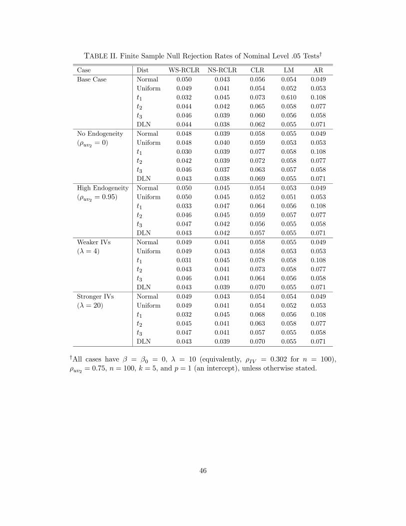
TABLE II. Finite Sample Null Rejection Rates of Nominal Level .05 Tests†

Case Dist WS-RCLR NS-RCLR CLR LM ARBase Case Normal 0.050 0.043 0.056 0.054 0.049

Uniform 0.049 0.041 0.054 0.052 0.053t1 0.032 0.045 0.073 0.610 0.108t2 0.044 0.042 0.065 0.058 0.077t3 0.046 0.039 0.060 0.056 0.058DLN 0.044 0.038 0.062 0.055 0.071

No Endogeneity Normal 0.048 0.039 0.058 0.055 0.049(ρuv2 = 0) Uniform 0.048 0.040 0.059 0.053 0.053

t1 0.030 0.039 0.077 0.058 0.108t2 0.042 0.039 0.072 0.058 0.077t3 0.046 0.037 0.063 0.057 0.058DLN 0.043 0.038 0.069 0.055 0.071

High Endogeneity Normal 0.050 0.045 0.054 0.053 0.049(ρuv2 = 0.95) Uniform 0.050 0.045 0.052 0.051 0.053

t1 0.033 0.047 0.064 0.056 0.108t2 0.046 0.045 0.059 0.057 0.077t3 0.047 0.042 0.056 0.055 0.058DLN 0.043 0.042 0.057 0.055 0.071

Weaker IVs Normal 0.049 0.041 0.058 0.055 0.049(λ = 4) Uniform 0.049 0.043 0.058 0.053 0.053

t1 0.031 0.045 0.078 0.058 0.108t2 0.043 0.041 0.073 0.058 0.077t3 0.046 0.041 0.064 0.056 0.058DLN 0.043 0.039 0.070 0.055 0.071

Stronger IVs Normal 0.049 0.043 0.054 0.054 0.049(λ = 20) Uniform 0.049 0.041 0.054 0.052 0.053

t1 0.032 0.045 0.068 0.056 0.108t2 0.045 0.041 0.063 0.058 0.077t3 0.047 0.041 0.057 0.055 0.058DLN 0.043 0.039 0.070 0.055 0.071

†All cases have β = β0 = 0, λ = 10 (equivalently, ρIV = 0.302 for n = 100),ρuv2 = 0.75, n = 100, k = 5, and p = 1 (an intercept), unless otherwise stated.

46

TABLE II. (cont.)

Case Dist WS-RCLR NS-RCLR CLR LM AROne IV Normal 0.048 0.041 0.053 0.053 0.050(k = 1) Uniform 0.052 0.045 0.055 0.055 0.053

t1 0.031 0.041 0.047 0.047 0.046t2 0.041 0.041 0.055 0.054 0.053t3 0.046 0.041 0.054 0.054 0.052DLN 0.045 0.047 0.057 0.057 0.054

Ten IVs Normal 0.052 0.048 0.053 0.052 0.050(k = 10, n = 200) Uniform 0.050 0.046 0.053 0.053 0.051

t1 0.032 0.051 0.058 0.044 0.127t2 0.049 0.048 0.058 0.050 0.090t3 0.049 0.045 0.054 0.052 0.062DLN 0.045 0.041 0.057 0.057 0.054

Smaller Sample Size Normal 0.045 0.036 0.061 0.056 0.048(n = 50) Uniform 0.050 0.039 0.065 0.058 0.050

t1 0.027 0.035 0.091 0.070 0.127t2 0.039 0.033 0.078 0.064 0.078t3 0.044 0.034 0.071 0.061 0.063DLN 0.044 0.037 0.076 0.064 0.074

Larger Sample Size Normal 0.048 0.046 0.052 0.052 0.049(n = 200) Uniform 0.049 0.044 0.052 0.052 0.053

t1 0.032 0.049 0.052 0.042 0.090t2 0.044 0.045 0.058 0.051 0.076t3 0.048 0.045 0.056 0.053 0.056DLN 0.050 0.046 0.056 0.054 0.067

47

TABLE III. Finite Sample Power of Size-corrected Level .05 Tests.†

Case Dist WS-RCLR NS-RCLR CLR LM ARBase Case Normal 0.42 0.46 0.40 0.40 0.26(β = 1.35) Uniform 0.41 0.48 0.40 0.40 0.25

t1 0.92 0.95 0.56 0.61 0.40t2 0.66 0.66 0.46 0.49 0.26t3 0.53 0.53 0.42 0.43 0.26DLN 0.61 0.60 0.43 0.45 0.23

Base Case Normal 0.35 0.35 0.39 0.38 0.25(β = −0.44) Uniform 0.32 0.38 0.39 0.39 0.25

t1 0.94 0.95 0.55 0.61 0.40t2 0.72 0.68 0.46 0.49 0.27t3 0.53 0.50 0.41 0.43 0.25DLN 0.65 0.59 0.42 0.44 0.22

Base Case Normal 0.38 0.40 0.39 0.39 0.26(β = 1.35 & β = −0.44) Uniform 0.37 0.43 0.40 0.40 0.25

t1 0.93 0.95 0.55 0.61 0.40t2 0.69 0.67 0.46 0.49 0.27t3 0.53 0.51 0.42 0.43 0.26DLN 0.63 0.60 0.42 0.44 0.23

No Endogeneity Normal 0.44 0.47 0.41 0.37 0.34(ρuv2 = 0, Uniform 0.43 0.47 0.42 0.37 0.34β = 0.975 & β = −1.05) t1 0.94 0.97 0.55 0.61 0.42

t2 0.74 0.72 0.46 0.47 0.33t3 0.57 0.56 0.43 0.40 0.34DLN 0.67 0.64 0.41 0.42 0.30

High Endogeneity Normal 0.38 0.39 0.41 0.41 0.22(ρuv2 = 0.95, Uniform 0.39 0.46 0.41 0.41 0.22β = 0.95 & β = −1.25) t1 0.93 0.96 0.61 0.64 0.41

t2 0.70 0.66 0.49 0.50 0.25t3 0.53 0.51 0.42 0.42 0.22DLN 0.67 0.62 0.44 0.44 0.19

†All cases have β0 = 0, λ = 10 (equivalently, ρIV = 0.302 for n = 100), ρuv2 = 0.75,n = 100, k = 5, and p = 1 (an intercept), unless otherwise stated.

48

TABLE III. (cont.)

Case Dist WS-RCLR NS-RCLR CLR LM ARWeaker IVs Normal 0.33 0.33 0.36 0.31 0.30(λ = 4, Uniform 0.31 0.33 0.36 0.32 0.29β = 25 & β = −0.725) t1 0.91 0.94 0.52 0.59 0.40

t2 0.61 0.58 0.41 0.43 0.28t3 0.43 0.42 0.37 0.35 0.29DLN 0.55 0.49 0.36 0.37 0.25

Stronger IVs Normal 0.40 0.42 0.40 0.40 0.23(λ = 20, Uniform 0.38 0.47 0.41 0.41 0.23β = 0.62 & β = −0.325) t1 0.94 0.96 0.58 0.63 0.40

t2 0.75 0.72 0.48 0.50 0.25t3 0.57 0.54 0.42 0.43 0.23DLN 0.59 0.54 0.38 0.40 0.22

One IV Normal 0.37 0.38 0.39 0.39 0.39(k = 1, Uniform 0.34 0.42 0.39 0.39 0.39β = 1.05 & β = −0.41) t1 0.88 0.89 0.44 0.44 0.44

t2 0.67 0.64 0.42 0.42 0.42t3 0.54 0.51 0.42 0.42 0.42DLN 0.66 0.61 0.40 0.40 0.40

Ten IVs Normal 0.38 0.39 0.41 0.41 0.24(k = 10, Uniform 0.38 0.43 0.45 0.45 0.27β = 1.9 & β = −0.49) t1 0.94 0.90 0.60 0.67 0.43

t2 0.72 0.69 0.50 0.54 0.28t3 0.54 0.52 0.46 0.46 0.28DLN 0.64 0.60 0.46 0.48 0.24

49