Randommatrixeigenvalueproblemsinstructuraldynamicsengweb.swan.ac.uk/~adhikaris/fulltext/journal/ft28.pdf · is based on a chi-square distribution. ... random eigenvalue problems;

INTERNATIONAL JOURNAL FOR NUMERICAL METHODS IN ENGINEERINGInt. J. Numer. Meth. Engng 2007; 69:562–591Published online 16 June 2006 in Wiley InterScience (www.interscience.wiley.com). DOI: 10.1002/nme.1781

Random matrix eigenvalue problems in structural dynamics

S. Adhikari∗,† and M. I. Friswell

Department of Aerospace Engineering, University of Bristol, Bristol BS8 1TR, U.K.

SUMMARY

Natural frequencies and mode shapes play a fundamental role in the dynamic characteristics of linearstructural systems. Considering that the system parameters are known only probabilistically, we obtainthe moments and the probability density functions of the eigenvalues of discrete linear stochastic dynamicsystems. Current methods to deal with such problems are dominated by mean-centred perturbation-basedmethods. Here two new approaches are proposed. The first approach is based on a perturbation expansionof the eigenvalues about an optimal point which is ‘best’ in some sense. The second approach is basedon an asymptotic approximation of multidimensional integrals. A closed-form expression is derived fora general rth-order moment of the eigenvalues. Two approaches are presented to obtain the probabilitydensity functions of the eigenvalues. The first is based on the maximum entropy method and the secondis based on a chi-square distribution. Both approaches result in simple closed-form expressions which canbe easily calculated. The proposed methods are applied to two problems and the analytical results arecompared with Monte Carlo simulations. It is expected that the ‘small randomness’ assumption usuallyemployed in mean-centred-perturbation-based methods can be relaxed considerably using these methods.Copyright q 2006 John Wiley & Sons, Ltd.

Received 2 August 2005; Revised 7 April 2006; Accepted 19 April 2006

KEY WORDS: random eigenvalue problems; asymptotic analysis; statistical distributions; randommatrices; linear stochastic systems

1. INTRODUCTION

Characterization of the natural frequencies and mode shapes play a key role in the analysis anddesign of engineering dynamic systems. The determination of natural frequency and mode shapesrequire the solution of an eigenvalue problem. Eigenvalue problems also arise in the context of the

∗Correspondence to: S. Adhikari, Department of Aerospace Engineering, University of Bristol, Queens Building,University Walk, Bristol BS8 1TR, U.K.

†E-mail: [email protected]

Contract/grant sponsor: Engineering and Physical Sciences Research Council (EPSRC); contract/grant number:GR/T03369/01Contract/grant sponsor: Royal Society

Copyright q 2006 John Wiley & Sons, Ltd.

RANDOM MATRIX EIGENVALUE PROBLEMS 563

stability analysis of structures. This problem could either be a differential eigenvalue problem or amatrix eigenvalue problem, depending on whether a continuous model or a discrete model is usedto describe the given vibrating system. Description of real-life engineering structural systems isinevitably associated with some amount of uncertainty in specifying material properties, geometricparameters, boundary conditions and applied loads. When we take account of these uncertainties,it is necessary to consider random eigenvalue problems. The solution of the random eigenvalueproblem is the first step to obtain the dynamic response statistics of linear stochastic systems.Random eigenvalue problems also arise in the stability analysis of linear systems with randomimperfections. Several studies have been conducted on this topic since the mid-1960s. The studyof probabilistic characterization of the eigensolutions of random matrix and differential operatorsis now an important research topic in the field of stochastic structural mechanics. The paper byBoyce [1], the book by Scheidt and Purkert [2] and the review papers by Ibrahim [3], Benaroya[4], Manohar and Ibrahim [5], and Manohar and Gupta [6] are useful sources of information onearly work in this area of research and also provide a systematic account of different approachesto random eigenvalue problems.

In this paper, discrete linear systems or discretized continuous systems are considered. Therandom eigenvalue problem of undamped or proportionally damped systems can be expressed by

K(x)/ j = � jM(x)/ j (1)

where � j and / j are the eigenvalues and the eigenvectors of the dynamic system. M(x) :Rm �→RN×N and K(x) :Rm �→ RN×N , the mass and stiffness matrices, are assumed to be smooth,continuous and at least twice differentiable functions of a random parameter vector x∈ Rm . Thevector x may consist of material properties, e.g. mass density, Poisson’s ratio, Young’s modulus;geometric properties, e.g. length, thickness, and boundary conditions. Statistical properties of thesystem are completely described by the joint probability density function px(x) :Rm �→ R. Formathematical convenience we express

px(x) = exp{−L(x)} (2)

where −L(x) is often known as the log-likelihood function. For example, if x is an m-dimensionalmultivariate Gaussian random vector with mean l∈ Rm and covariance matrix R∈ Rm×m then

L(x) = m

2ln(2�) + 1

2ln ‖R‖ + 1

2(x − l)TR−1(x − l) (3)

It is assumed that in general the random parameters are non-Gaussian and correlated, i.e. L(x)can have any general form provided it is a smooth, continuous and at least twice differentiablefunction. It is further assumed that M and K are symmetric and positive definite random matricesso that all the eigenvalues are real and positive.

The central aim of studying random eigenvalue problems is to obtain the joint probability densityfunction of the eigenvalues and the eigenvectors. The current literature on random eigenvalueproblems arising in engineering systems is dominated by the mean-centred perturbation methods[7–16]. These methods work well when the uncertainties are small and the parameter distributionis Gaussian. In theory, any set of non-Gaussian random variables can be transformed into a setof standard Gaussian random variables by using numerical transformations such as the Rosenblatttransformation or the Nataf transformation. These transformations are however often complicated,numerically expensive and inconvenient to implement in practice. Some authors have proposed

Copyright q 2006 John Wiley & Sons, Ltd. Int. J. Numer. Meth. Engng 2007; 69:562–591DOI: 10.1002/nme

564 S. ADHIKARI AND M. I. FRISWELL

methods which are not based on the mean-centred perturbation method. Grigoriu [17] examinedthe roots of characteristic polynomials of real symmetric random matrices using the distributionof zeros of random polynomials. Lee and Singh [18] proposed a direct matrix product (Kroneckerproduct) method to obtain the first two moments of the eigenvalues of discrete linear systems.More recently Nair and Keane [19] proposed a stochastic reduced basis approximation whichcan be applied to discrete or discretized continuous dynamic systems. Hala [20] and Mehlhoseet al. [21] used a Ritz method to obtain closed-form expressions for moments and probabilitydensity functions of the eigenvalues (in terms of Chebyshev–Hermite polynomials). Szekely andSchueller [22], Pradlwarter et al. [23] and Du et al. [24] considered simulation-based methodsto obtain eigensolution statistics of large systems. Ghosh et al. [25] used a polynomial chaosexpansion for random eigenvalue problems. Adhikari [26] considered complex random eigenvalueproblems associated with non-proportionally damped systems. Recently, Verhoosel et al. [27]proposed an iterative method that can be applied to non-symmetric random matrices also. Rahman[28] developed a dimensional decomposition method which does not require the calculation ofeigensolution derivatives.

Under special circumstances when the matrix H=M−1K∈ RN×N is Gaussian unitary ensemble(GUE) or Gaussian orthogonal ensemble (GOE) an exact closed-form expression can be obtainedfor the joint pdf of the eigenvalues using random matrix theory (RMT). See the book by Mehta [29]and references therein for discussions on RMT. RMT has been extended to other type of randommatrices. If H has Wishart distribution then the exact joint pdf of the eigenvalues can be obtainedfrom Muirhead [30, Theorem 3.2.18]. Edelman [31] obtained the pdf of the minimum eigenvalue(first natural frequency squared) of a Wishart matrix. A more general case when the matrix H has�-distribution has been obtained by Muirhead [30, Theorem 3.3.4] and more recently by Dumitriuand Edelman [32]. Unfortunately, the system matrices of real structures may not always followsuch distributions and consequently some kind of approximate analysis is required.

In this paper, two new approaches are proposed to obtain the moments and probability densityfunctions of the eigenvalues. The first approach is based on a perturbation expansion of theeigenvalues about a point in the x-space which is ‘optimal’ is some sense (and in general differentfrom the mean). The second approach is based on asymptotic approximation of multidimensionalintegrals. The proposed methods do not require the ‘small randomness’ assumption or Gaussianpdf assumption of the basic random variables often employed in literature. Moreover, they alsoeliminate the need to use intermediate numerical transformations of the basic random variables.In Section 2, perturbation-based methods are discussed. In Section 2.1, mean-centred perturbationmethods are briefly reviewed. The perturbation method based on an optimal point is discussedin Section 2.2. In Section 3, a new method to obtain arbitrary order moments of the eigenvaluesis proposed. Using these moments, some closed-form expressions of approximate pdf of theeigenvalues are derived in Section 4. In Section 5, the proposed analytical methods are applied totwo problems and the results are compared with Monte Carlo simulations.

2. STATISTICS OF THE EIGENVALUES USING PERTURBATION METHODS

2.1. Mean-centred perturbation method

2.1.1. Perturbation expansion. The mass and the stiffness matrices are in general non-linear func-tions of the random vector x. Denote the mean of x as l∈ R, and consider that

M(l) =M and K(l) =K (4)



are the ‘deterministic parts’ of the mass and stiffness matrices, respectively. In general M and Kare different from the mean matrices. The deterministic part of the eigenvalues:

� j = � j (l) (5)

is obtained from the deterministic eigenvalue problem:

K/ j = � j M/ j (6)

The eigenvalues, � j (x) :Rm �→ R are non-linear functions of the parameter vector x. If the eigenval-ues are not repeated, then each � j (x) is expected to be a smooth and twice differentiable functionsince the mass and stiffness matrices are smooth and twice differentiable functions of the randomparameter vector. In the mean-centred perturbation approach, the function � j (x) is expanded byits Taylor series about the point x= l as

� j (x) ≈ � j (l) + dT� j(l)(x − l) + 1

2 (x − l)TD� j (l)(x − l) (7)

Here d� j (l) ∈ Rm and D� j (l) ∈ Rm×m are, respectively, the gradient vector and the Hessian matrixof � j (x) evaluated at x= l, that is

{d� j (l)}k = �� j (x)

�xk

∣∣∣∣x=l

(8)

and

{D� j (l)}kl =�2� j (x)

�xk�xl

∣∣∣∣∣x=l

(9)

Expressions for the elements of the gradient vector and the Hessian matrix are given in Section A.1.Due to Equation (5), Equation (7) implies that the eigenvalues are effectively expanded about theircorresponding deterministic value � j .

Equation (7) represents a quadratic form in basic non-Gaussian random variables. The first-order perturbation, which is often used in practice, is obtained from Equation (7) by neglectingthe Hessian matrix. In this case, the eigenvalues are simple linear functions of the basic randomvariables. This formulation is expected to produce acceptable results when the random variationin x is small. If the basic random variables are Gaussian, then first-order perturbation results ina Gaussian distribution of the eigenvalues. In this case, a closed-form expression for their jointprobability density function can be obtained easily, see for example, Reference [7]. Recently,Adhikari [26] used the first-order perturbation method for complex eigenvalue problems arisingin non-proportionally damped systems. However, if the elements of x are non-Gaussian then eventhe first-order perturbation method is not helpful because there is no general method to obtain theresulting pdf in a simple manner.

When the second-order terms are retained in Equation (7), each � j (x) results in a quadraticform in x. If the elements of x are Gaussian, then it is possible to obtain descriptive statistics usingthe theory of quadratic forms as discussed next.

2.1.2. Eigenvalue statistics using theory of quadratic forms. Extensive discussions on quadraticforms in Gaussian random variables can be found in the books by Johnson and Kotz [33, Chapter 29]



and Mathai and Provost [34]. Using the methods outlined in these references moments/cumulantsof the eigenvalues are obtained in this section.

When x is a multivariate Gaussian random vector, the moment generating function of � j (x), forany s ∈ C, can be obtained from Equation (7) as

M� j (s) = E[exp{s� j (x)}]

=∫

Rmexp{s� j (l) + sdT� j

(l)(x − l) + s

2(x − l)TD� j (l)(x − l) − L(x)} dx (10)

where L(x) is given by Equation (3). Using the transformation

y= (x − l) (11)

the integral in Equation (10) can be evaluated exactly as

M� j (s) = (2�)−m/2‖R‖−1/2∫

Rmexp

{s� j + sdT� j

(l)y−1

2yT[R−1−sD� j (l)]y

}dy (12)

or

M� j (s) =exp{s� j + (s2/2)dT� j

(l)R[I − sR D� j (l)]−1d� j (l)}√‖I − sRD� j (l)‖

(13)

To obtain the pdf of � j (x), the inverse Laplace transform of Equation (13) is required. The exactclosed-form expression of the pdf can be obtained for few special cases only. Some approximatemethods to obtain the pdf of � j (x) will be discussed in Section 4.

If the mean-centred first-order perturbation is used then D� j (l) =O and from Equation (13) weobtain

M� j (s) ≈ exp

{s� j + s2

2dT� j

(l)Rd� j (l)

}(14)

This implies that � j (x) is a Gaussian random variable with mean � j and variance dT� j(l)Rd� j (l).

However, for second-order perturbations in general the mean of the eigenvalues is not the deter-ministic value. The cumulants of � j (x) can be obtained from

�(r)j = dr

dsrlnM� j (s)|s=0 (15)

Here �(r)j is the r th-order cumulant of j th eigenvalue and from Equation (13) we have

lnM� j (s) = s� j + s2

2dT� j

(l)R[I − sRD� j (l)]−1d� j (l) − 1

2ln ‖I − sRD� j (l)‖ (16)

Using this expression and after some simplifications it can be shown that

�(r)j = � j + 1

2Trace(D� j (l)R) if r = 1 (17)



�(r)j = r !

2dT� j

(l)[RD� j (l)]r−2Rd� j (l) + (r − 1)!2

Trace([D� j (l)R]r ) if r�2 (18)

The mean and first few cumulants of the eigenvalues can be explicitly obtained as

� j = �(1)j = � j + 1

2Trace(D� j (l)R) (19)

Var[� j ] = �(2)j =dT� j

(l)Rd� j (l) + 12 Trace([D� j (l)R]2) (20)

�(3)j = 3dT� j

(l)[RD� j (l)]Rd� j (l) + Trace([D� j (l)R]3) (21)

and

�(4)j = 12dT� j

(l)[RD� j (l)]2Rd� j (l) + 3Trace([D� j (l)R]4) (22)

From the cumulants, the raw moments �(r)j = E[�rj ] and the central moments �′(r)

j = E[(� j − � j )r ]

can be obtained using standard formulae [35, Chapter 26].

2.2. Perturbation method based on an optimal point

2.2.1. Perturbation expansion. In the mean-centred perturbation method, � j (x) is expanded in aTaylor series about x= l. This approach may not be suitable for all problems, especially if x isnon-Gaussian then px(x) may not be centred around the mean. Here we are looking for a pointx= a in the x-space such that the Taylor series expansion of � j (x) about this point

� j (x) ≈ � j (a) + dT� j(a)(x − a) + 1

2 (x − a)TD� j (a)(x − a) (23)

is optimal in some sense. The idea of the optimal point is related to the saddle point approximation,see for example the book by MacKay [36, Chapter 29]. The optimal point a can be selected invarious ways. For practical applications the mean of the eigenvalues is often the most important. Forthis reason, the optimal point a is selected such that the mean or the first moment of each eigenvalueis calculated most accurately. The mathematical formalism presented here is not restricted to thisspecific criteria and can be easily modified if any moment other than the first moment is requiredto be obtained more accurately. Using Equation (2), the mean of � j (x) can be obtained as

� j = E[� j (x)] =∫

Rm� j (x)px(x) dx=

∫Rm

� j (x)e−L(x) dx (24)

or

� j =∫

Rme−h j (x) dx (25)

where

h j (x)= L(x) − ln � j (x) (26)

Evaluation of integral (25), either analytically or numerically, is in general difficult because (a)� j (x) and L(x) are complicated non-linear functions of x, (b) an explicit functional form � j (x)



is not easy to obtain except for very simple problems (usually an FE run is required to obtain� j for every x), and (c) the dimension of the integral m is large. For these reasons some kindof approximation is required. From Equation (25), note that the maximum contribution to theintegral comes from the neighbourhood where h j (x) is minimum. Therefore, the function h j (x)is expanded in a Taylor series about the point where h j (x) has its global minimum. By doing so,the error in evaluating integral (25) would be minimized. Thus, the optimal point can be obtainedfrom

�h j (x)

�xk= 0 or

�L(x)�xk

= 1

� j (x)�� j (x)

�xk∀k (27)

Combining the above equation for all k, at x= a we have

d� j (a) = � j (a)dL(a) (28)

Equation (28) implies that at the optimal point the gradient vectors of the eigenvalues and log-likelihood function are parallel. The non-linear set of equations (28) have to be solved numerically.Due to the explicit analytical expression of d� j in terms of the derivative of the mass and stiffnessmatrices, expensive numerical differentiation of � j (x) at each step is not needed. Moreover, formost px(x), a closed-form expression of dL(x) is available. For example, when x has multivariateGaussian distribution, L(x) is given by Equation (3). By differentiating this, we obtain

dL(x)=R−1(x − l) (29)

Substituting this in Equation (28), the optimal point a can be obtained as

a= l+ 1

� j (a)Rd� j (a) (30)

This equation also gives a recipe for an iterative algorithm to obtain a. One starts with an initial a inthe right-hand side and obtains an updated a in the left-hand side. This procedure can be continueduntil the difference between the values of a obtained from both sides of Equation (30) is less than(l2 vector norm can be used to measure the difference) a predefined small value. A good value tostart the iteration process is a= l, as in the case of mean-centred approach. Note that the solutionof a deterministic eigenvalue problem is needed at each step of the iteration process. The formof Equation (23) is similar to that of Equation (7). As mentioned before, when the basic randomvariables are non-Gaussian, determination of moments and the pdf is not straightforward. However,when x is Gaussian, some useful statistics of the eigenvalues can be obtained in closed-form.

2.2.2. Eigenvalue statistics using theory of quadratic forms. For notational convenience we rewritethe optimal perturbation expansion (23) as

� j (x) ≈ c j + aTj x + 12x

TA jx (31)

where the constants c j ∈ R, a j ∈ Rm and A j ∈ Rm×m are given by

c j = � j (a) − dT� j(a)a+ 1

2aTD� j (a)a (32)

a j = d� j (a) − D� j (a)a (33)



A j =D� j (a) (34)

From Equation (31), the closed-form expression of the moment generating function of � j (x) canbe obtained exactly in a way similar to that for the case of the mean-centred perturbation method.Using Equation (3), it can be shown that

M� j (s) = E[exp{s� j (x)}]

= (2�)−m/2‖R‖−1/2∫

Rmexp{s(c j + aTj x + 1

2xTA jx)

− 12 (x − l)TR−1(x − l)} dx (35)

This m-dimensional integral can be evaluated exactly to obtain

M� j (s)= exp{sc j − 12l

TR−1l+ 12 (l+ sRa j )

T[I − sRA j ]−1(l+ sRa j )}√‖I − sRA j‖(36)

From the preceeding expression, the cumulants of the eigenvalues can be evaluated usingEquation (15) as

�(r)j = c j + 1

2 Trace(A jR) + 12l

TA jl+ aTj l if r = 1 (37)

and

�(r)j = (r − 1)!

2Trace([A jR]r ) + r !

2aTj [RA j ]r−2Ra j

+ r !lT[A jR]r−1A jl+ r !aTj [RA j ]r−1A jl if r�2 (38)

The mean and first few cumulants of the eigenvalues can be explicitly obtained as

� j = �(1)j = c j + 1

2Trace(A jR) + 12l

TA jl+ aTj l (39)

Var[� j ] = �(2)j = 1

2 Trace([A jR]2) + aTjRa j + 2lT[A jR]A jl+ 2aTj [RA j ]A jl (40)

�(3)j = Trace([A jR]3) + 3aTj [RA j ]a j + 6lT[A jR]2A jl+ 6aTj [RA j ]2A jl (41)

and

�(4)j = 3Trace([A jR]4) + 12aTj [RA j ]2a j + 24lT[A jR]3A jl+ 24aTj [RA j ]3A jl (42)

Since Equations (17), (18), (37) and (38) gives cumulants of arbitrary order, it is possible toreconstruct the pdf of the eigenvalues from them. However, when the elements of x are non-Gaussian, then neither the first-order perturbation nor the second-order perturbation methods arehelpful because there is no general method to obtain the resulting statistics in a simple manner. Insuch cases, the method outlined in the next section might be more useful.



3. METHOD BASED ON THE ASYMPTOTIC INTEGRAL

3.1. Multidimensional integrals in unbounded domains

In this section, the moments of the eigenvalues are obtained based on an asymptotic approximationof the multidimensional integral. Consider a function f (x) : Rm �→ R which is smooth and at leasttwice differentiable. Suppose we want to evaluate an integral of the following form:

J=∫

Rmexp{− f (x)} dx (43)

This is an m-dimensional integral over the unbounded domain Rm . The maximum contribution tothis integral comes from the neighbourhood where f (x) reaches its global minimum. Suppose thatf (x) reaches its global minimum at a unique point h∈ Rm . Therefore, at x= h

� f (x)�xk

= 0 ∀k or d f (h) = 0 (44)

Using this, f (x) is expanded in a Taylor series about h and Equation (43) is rewritten as

J=∫

Rmexp{−{ f (h) + 1

2 (x − h)TD f (h)(x − h) + �(x, h)}} dx

= exp{− f (h)}∫

Rmexp{− 1

2 (x − h)TD f (h)(x − h) − �(x, h)} dx (45)

where �(x, h) is the error if only the terms up to second-order were retained in the Taylor seriesexpansion. With suitable scaling of x the integral in Equation (43) can be transformed to theso-called ‘Laplace integral’. Under special conditions, such integrals can be well approximatedusing asymptotic methods. The relevant mathematical methods and formal derivations are coveredin detail in the books by Bleistein and Handelsman [37] and Wong [38]. Here we propose asomewhat different version of the asymptotic integrals. The error �(x, h) depends on higher orderderivatives of f (x) at x= h. If they are small compared to f (h) and the elements of D f (h), theircontribution will be negligible to the value of the integral. Therefore, we assume f (h) and theelements of D f (h) are large so that∣∣∣∣ 1

f (h)D( j)( f (h))

∣∣∣∣ → 0 and ∀k, l,∣∣∣∣ 1

[D f (h)]kl D( j)( f (h))

∣∣∣∣ → 0 for j>2 (46)

where D( j)( f (h)) is j th-order derivative of f (x) evaluated at x= h. Under such assumptions,�(x, h) → 0. Therefore, the integral in (45) can be approximated as

J≈ exp{− f (h)}∫

Rmexp{− 1

2 (x − h)TD f (h)(x − h)} dx (47)

If h is the global minimum of f (x) in Rm , the symmetric Hessian matrix D f (h) ∈ Rm×m is alsoexpected to be positive definite. Now use the coordinate transformation

n= (x − h)D−1/2f (h) (48)



The Jacobian of this transformation is

‖J‖=‖D f (h)‖−1/2 (49)

Using Equation (48), the integral in Equation (47) can be evaluated as

J≈ exp{− f (h)}∫

Rm‖D f (h)‖−1/2 exp{− 1

2 (nTn)} dn (50)

or

J≈ (2�)m/2 exp{− f (h)}‖D f (h)‖−1/2 (51)

The analysis proposed here is somewhat different from the widely used Laplace’s method ofasymptotic approximation of integrals [38, Chapter IX, Theorem 3]. Here it is simply assumedthat the higher order derivativesD( j)( f (h)) are negligibly small compared to f (h) and the elementsof D f (h). This approximation is expected to yield good results if the minimum of f (x) aroundx= h is sharp. If h is not unique then it is required to sum the contributions arising from all suchoptimal points separately. Equation (51) will now be used to obtain moments of the eigenvalues.

3.2. Calculation of an arbitrary moment of the eigenvalues

An arbitrary r th-order moment of the eigenvalues can be obtained from

�(r)j = E[�rj (x)] =

∫Rm

�rj (x)px(x) dx

=∫

Rmexp{−(L(x) − r ln � j (x))} dx, r = 1, 2, 3, . . . (52)

The equation can be expressed in the form of Equation (43) by choosing

f (x)= L(x) − r ln � j (x) (53)

Differentiating the above equation with respect to xk , we obtain

� f (x)�xk

= �L(x)�xk

− r

� j (x)�� j (x)

�xk(54)

The optimal point h can be obtained from Equation (44) by equating the above expression to zero.Therefore at x= h

� f (x)

�xk= 0 ∀k (55)

or

r

� j (h)

�� j (h)

�xk= �L(h)

�xk∀k (56)

or

d� j (h)r = � j (h)dL(h) (57)



Equation (57) is similar to Equation (28) and needs to solved numerically to obtain h. The stepsto obtain h are similar to those described in Section 2.2.

The elements of the Hessian matrix D f (h) can be obtained by differentiating Equation (54)with respect to xl :

�2 f (x)�xk�xl

= �2L(x)�xk�xl

− r

(− 1

�2j (x)

�� j (x)

�xl

�� j (x)

�xk+ 1

� j (x)�2� j (x)

�xk�xl

)

= �2L(x)�xk�xl

+ 1

r

{r

� j (x)�� j (x)

�xk

}{r

� j (x)�� j (x)

�xl

}− r

� j (x)�2� j (x)

�xk�xl(58)

At x= h we can use Equation (56) so that Equation (58) reads

�2 f (x)�xk�xl

∣∣∣∣∣x=h

= �2L(h)

�xk�xl+ 1

r

�L(h)

�xk

�L(h)

�xl− r

� j (h)

�2� j (h)

�xk�xl(59)

Combining this equation for all k and l we have

D f (h) =DL(h) + 1

rdL(h)dL(h)T − r

� j (h)D� j (h) (60)

where D� j (•) is defined in Equation (9). Using the asymptotic approximation (51), the r th momentof the eigenvalues can be obtained as

�(r)j ≈ (2�)m/2�rj (h) exp{−L(h)}

∥∥∥∥DL(h) + 1

rdL(h)dL(h)T − r

� j (h)D� j (h)

∥∥∥∥−1/2

(61)

This is perhaps the most general formula to obtain the moments of the eigenvalues of linearstochastic dynamic systems. The optimal point h needs to be calculated by solving non-linearset of equations (57) for each � j and r . Several special cases arising from Equation (61) are ofpractical interest:

• Mean of the eigenvalues: The mean of the eigenvalues can be obtained by substituting r = 1in Equation (61), that is

� j = �(1)j = (2�)m/2� j (h) exp{−L(h)}‖DL(h) + dL(h)dL(h)T − D� j (h)/� j (h)‖−1/2

(62)

• Central moments of the eigenvalues: Once the mean is known, the central moments can beexpressed in terms of the raw moments �(r)

j using the binomial transform

�′(r)j = E[(� j − � j )

r ] =r∑

k=0

(r

k

)(−1)r−k�(k)

j �r−kj (63)



• Random vector x has multivariate Gaussian distribution: In this case L(x) is given byEquation (3) and by differentiating Equation (29) we obtain

DL(x)=R−1 (64)

The optimal point h can be obtained from Equation (57) as

h= l+ r

� j (h)Rd� j (h) (65)

Using Equations (29) and (64), the Hessian matrix can be derived from Equation (60) as

D f (h) =R−1 + 1

rR−1(h− l)(h− l)TR−1 − r

� j (h)D� j (h)

=R−1(I + 1

r(h− l)(h− l)TR−1

)− r

� j (h)D� j (h) (66)

Therefore, the r th moment of the eigenvalues can be obtained from Equation (61) as

�(r)j ≈ �rj (h) exp{− 1

2 (h− l)TR−1(h− l)}‖R‖−1/2‖D f (h)‖−1/2 (67)

Using Equation (66) and recalling that for any two matrices A and B, ‖A‖‖B‖= ‖AB‖ we have

�(r)j ≈ �rj (h) exp{− 1

2 (h− l)TR−1(h− l)}‖I + D f (h)‖−1/2(68)

where

D f (h) = 1

r(h− l)(h− l)TR−1 − r

� j (h)RD� j (h) (69)

The probability density function of the eigenvalues is considered in the next section.

4. PROBABILITY DENSITY FUNCTION OF THE EIGENVALUES

4.1. Maximum entropy probability density function

Once the cumulants/moments of the eigenvalues are known, the pdf of the eigenvalues can beobtained using the maximum entropy method (MEM). Because Equations (17), (18), (37), (38)and (61) can be used to calculate any arbitrary order cumulant and moment, the pdf can beobtained accurately by taking higher order terms. Here, following Kapur and Kesavan [39], ageneral approach is presented.

Since M and K are symmetric and positive definite random matrices, all the eigenvalues are realand positive. Suppose the pdf of � j is given by p� j (u) where u ∈ R is positive, that is u ∈ [0,∞].Considering that only first n moments are used, the pdf of each eigenvalue must satisfy thefollowing constraints: ∫ ∞

0p� j (u) du = 1 (70)



and ∫ ∞

0ur p� j (u) du = �(r)

j , r = 1, 2, 3, . . . , n (71)

Using Shannon’s measure of entropy

S=−∫ ∞

0p� j (u) ln p� j (u) du (72)

we construct the Lagrangian

L= −∫ ∞

0p� j (u) ln p� j (u) du − (�0 − 1)

[∫ ∞

0p� j (u) du − 1

]

−n∑

r=1�r

[∫ ∞

0ur p� j (u) du − �(r)

j

](73)

where �r , r = 0, 1, 2, . . . , n are Lagrange multipliers. The function p� j (u) which maximizes Lcan be obtained using the calculus of variations. Using the Euler–Lagrange equation the solutionis given by

p� j (u) = exp

{−�0 −

n∑i=1

�i ui}

= exp{−�0

}exp

{−

n∑i=1

�i ui}

, u�0 (74)

The Lagrange multipliers can be obtained from the constraint equations ((70) and (71)) as

exp{�0} =∫ ∞

0exp

{−

n∑i=1

�i ui}du (75)

and

exp{�0}�(r)j =

∫ ∞

0ur exp

{−

n∑i=1

�i ui}du for r = 0, 1, 2, . . . , n (76)

Closed-form expressions for �r are in general not possible for all n. If we take n = 2, then theresulting pdf can be expressed as the truncated Gaussian density function

p� j (u) = 1√2�� j�(� j/� j )

exp

{− (u − � j )

2

2�2j

}, u�0 (77)

where � j is given by

�2j = �(2)j − �

2j (78)

The approach presented above can also be used in conjunction with the perturbation methods bytransforming the cumulants obtained from Equations (17), (18), (37) and (38) to moments. Thetruncated Gaussian density function derived here ensures that the probability of any eigenvaluesbecoming negative is zero.



4.2. Approximation by 2 probability density function

We use an approximation analogous to Pearson’s [40] three moment central 2 approximation tothe distribution of a noncentral 2. The eigenvalues are approximated as

� j ≈ j + � j2� j (u) (79)

where 2� j (u) is a central 2 density function with � j degrees of freedom (see Reference [35,Chapter 26]). The constants j , � j , and � j are obtained such that the first three moments of � j areequal to that of the approximated 2 pdf. The moment generating function of the approximated 2

pdf is given by

E[exp{−s( j + � j2� j )}] = exp{−s j }(1 + 2s� j )

−� j /2 (80)

Equating the first three moments we have

j + � j� j = �(1)j (81)

2j + 2 j� j� j + �2j�2j + 2� j�

2j = �(2)

j (82)

and

3j + 32j� j� j + 3 j�2j�

2j + 6 j� j�

2j + �3j�

3j + 6�2j�

3j + 8� j�

3j = �(3)

j (83)

This set of coupled non-linear equations can be solved exactly in closed-form to obtain j , � j ,and � j :

j = �(1)j

2�(2)j − 2�(2)

j

2 + �(1)j �(3)

j

2�(1)j

3 − 3�(1)j �(2)

j + �(3)j

(84)

� j = 2�(1)j

3 − 3�(1)j �(2)

j + �(3)j

4(�(2)j − �(1)

j

2)

(85)

and

� j = 8(�(2)

j − �(1)j

2)3

(2�(1)j

3 − 3�(1)j �(2)

j + �′3)

2(86)

Moments of � j (x) obtained in Equation (61), can be used directly in the right-hand side ofthese equations. Alternatively, this approach can also be used in conjunction with the perturbationmethods by transforming the cumulants obtained from Equations (17), (18), (37) and (38) tomoments. Using the transformation in Equation (79), the approximate probability density functionof � j (x) is given by

p� j (u) ≈ 1

� jp2� j

(u − j

� j

)= (u − j )

� j /2−1 exp{−(u − j )/2� j }(2� j )

� j /2�(� j/2)(87)



The two approximated pdf proposed here have simple forms but it should be noted that they arenot exhaustive. Given the moments/cumulants, different probability density functions can be fittedusing different methods. The application of the approximate pdfs derived here is illustrated in thenext section.

5. APPLICATION EXAMPLES

5.1. A two-DOF system

5.1.1. System model and computational methodology. A simple two-degree-of-freedom undampedsystem has been considered to illustrate a possible application of the expressions developed so far.The main purpose of this example is to understand how the proposed methods compare with theexisting methods. Figure 1 shows the example, together with the numerical values of the massesand spring stiffnesses. The system matrices for the example are given by

M=[m1 0

0 m2

]and K=

[k1 + k3 −k3

−k3 k2 + k3

](88)

It is assumed that only the stiffness parameters k1 and k2 are uncertain so that ki =ki (1+�i xi ), i = 1, 2 and ki denote the deterministic values of the spring constants. Here x={x1, x2}T∈ R2 is a vector of standard Gaussian random variables, that is l= 0 and R= I. The numericalvalues of the ‘strength parameters’ are considered as �1 = �2 = 0.25. The strength parameters areselected so that the system matrices are almost surely positive definite. Noting that M is indepen-dent of x and K is a linear function of x, the derivative of the system matrices with respect to therandom vector x can be obtained as

�K�x1

= �1

⎡⎣ k1 0

0 0

⎤⎦ ,�K�x2

= �2

⎡⎣0 0

0 k2

⎤⎦ (89)

�M�xi

=O and�2K

�xi�x j=O (90)

We calculate the raw moments and the probability density functions of the two eigenvalues ofthe system. Recall that the eigenvalues obtained from Equation (1) are the square of the natural

m m2

k k23k1

1

1 2

Figure 1. The undamped two-degree-of-system, m1 = 1 kg, m2 = 1.5 kg, k1 = 1000N/m,k2 = 1100N/m and k3 = 100N/m.



frequencies (� j = 2j ). The following six methods are used to obtain the moments and the pdfs:

1. Mean-centred first-order perturbation: This case arises when D� j (l) in the Taylor seriesexpansion (7) is assumed to be a null matrix so that only the first-order terms are retained.This is the simplest approximation, and as mentioned earlier, results in a Gaussian distributionof the eigenvalues. Recalling that for this problem, l= 0 and R= I, the resulting statisticsfor this special case can be obtained from Equations (19) and (20) as

� j = � j (91)

and

Var[� j ] =dT� j(0)d� j (0) (92)

The gradient vector d� j (0) can be obtained from Equation (A2) using the system derivativematrices (89) and (90).

2. Mean-centred second-order perturbation: In this case all the terms in Equation (7) are retained.This approximation results in a quadratic form in the Gaussian random variables. The resultingstatistics can be obtained from Equations (17) and (18) by substituting l= 0 and R= I. Theelements of the Hessian matrix D� j (0) can be obtained from Equation (A4) and using thesystem derivative matrices (89) and (90).

3. Optimal point first-order perturbation: This case arises when D� j (a) in the Taylor seriesexpansion (23) is assumed to be a null matrix so that only the first-order terms are retained.Like its mean-centred counterpart, this approach also results in a Gaussian distribution of theeigenvalues. From Equation (31) we have

c j = � j (a) − dT� j(a)a, a j =d� j (a) and A j =O (93)

The equation for the optimal point a is obtained from Equation (30) as

a=d� j (a)/� j (a) or d� j (a) = � j (a)a (94)

Using these equations, the mean and the variance can be obtained as special cases ofEquations (39) and (40) as

� j = � j (a) − dT� j(a)a= � j (a) − � j (a)a

Ta (95)

or

� j = � j (a)(1 − |a|2) (96)

and

Var[� j ] =dT� j(a)d� j (a) = �2j (a)|a|2 (97)

4. Optimal point second-order perturbation: In this case all the terms in Equation (23) areretained. Like the mean-centred approach, this approximation also results in a quadratic formin the Gaussian random variables, but with different coefficients. The resulting statistics canbe obtained from Equations (37) and (38).



5. Method based on the asymptotic integral: In this case, the moments can be obtained usingEquation (61). For the standardized Gaussian random vector, substituting l= 0 and R= I inEquation (67) the moment formula can be simplified to

�(r)j ≈ �rj (h) exp

{−1

2|h|2

}∥∥∥∥I + 1

rhhT/r − r

� j (h)D� j (h)

∥∥∥∥−1/2

(98)

and

h= rd� j (h)/� j (h), r = 1, 2, 3, . . . (99)

The vector h needs to be calculated for each r and j from Equation (99) using the iterativeapproach discussed before. The moments obtained from Equation (98) can be used to obtainthe pdf using the approach given in Section 4.

6. Monte Carlo simulation: The samples of two independent Gaussian random variables x1 andx2 are generated and the eigenvalues are computed directly from Equation (1). A total of15 000 samples are used to obtain the statistical moments and pdf of both the eigenvalues.The results obtained from the Monte Carlo simulation are assumed to be the benchmark forthe purpose of comparing the five analytical methods described above.

5.1.2. Numerical results. Figure 2 shows the percentage error for the first four raw moments ofthe first eigenvalue. The percentage error for an arbitrary kth moment of an eigenvalue obtainedusing any one of the five analytical methods is given by

Errori th method = |{�(r)j }i th method − {�(r)

j }MCS|{�(r)

j }MCS

× 100, i = 1, . . . , 5 (100)

1 2 3 40

2

4

6

8

10

12

14

16

18

20

[λk1]

Perc

enta

ge e

rror

wrt

MC

S

Asymptotic Method

Figure 2. Percentage error for the first eigenvalue.



1 2 3 40

1

2

3

4

5

6

7

8

9

10

[λk2]

Perc

enta

ge e

rror

wrt

MC

S

Asymptotic Method

Figure 3. Percentage error for the second eigenvalue.

Figure 3 shows the percentage error for the first four raw moments of the second eigenvalue. Forboth eigenvalues, the error corresponding to the mean-centred first-order perturbation method ismore than the other four methods. The error corresponding to the optimal point first-order pertur-bation method follows next. Moments obtained from mean-centred and optimal point second-orderperturbation methods are more accurate compared to their corresponding first-order counterparts.In general, the moments obtained from the asymptotic formula equation (61) turn out to be quiteaccurate. The absolute errors for the second eigenvalue are less compared to the first eigenvalue.For the first eigenvalue, the moments obtained from the asymptotic formula turn out to be the mostaccurate, while for the second eigenvalue, the mean-centred second-order perturbation methodyields the most accurate results.

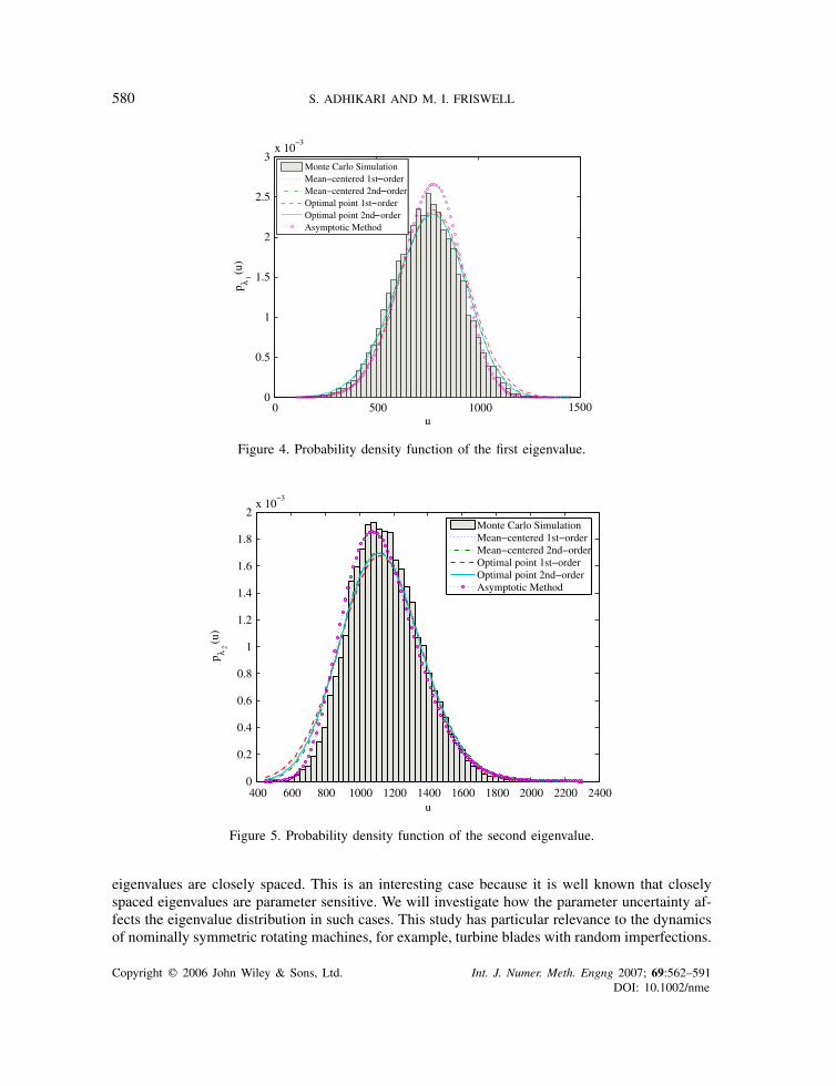
Now consider the probability density function of the eigenvalues. Figures 4 and 5, respec-tively, show the pdf of the first and the second eigenvalue obtained from the five methodsdescribed earlier. The pdf corresponding to first five methods are obtained using the 2 dis-tribution in Equation (87). The constants appearing in this equation are calculated from themoments using Equations (84)–(86). In the same plots, the normalized histograms of the eigen-values obtained from the Monte Carlo simulation are also plotted. For the first eigenvalue, thepdf from the second-order perturbation methods are accurate in the lower and in the upper tail.For the second eigenvalue, the pdf from the asymptotic moment method is accurate over thewhole curve.

5.2. A three-DOF system with closely spaced eigenvalues

5.2.1. System model and computational methodology. A three-degree-of-freedom undampedspring–mass system, taken from Reference [41], is shown in Figure 6. The main purposeof this example is to understand how the proposed methods work when some of the system



0 500 1000 15000

0.5

1

1.5

2

2.5

3x 10

u

p λ 1 (u)

Monte Carlo Simulation

Asymptotic Method

Figure 4. Probability density function of the first eigenvalue.

400 600 800 1000 1200 1400 1600 1800 2000 2200 24000

0.2

0.4

0.6

0.8

1

1.2

1.4

1.6

1.8

2x 10

u

p λ2 (

u)

Monte Carlo Simulation

Asymptotic Method

Figure 5. Probability density function of the second eigenvalue.

eigenvalues are closely spaced. This is an interesting case because it is well known that closelyspaced eigenvalues are parameter sensitive. We will investigate how the parameter uncertainty af-fects the eigenvalue distribution in such cases. This study has particular relevance to the dynamicsof nominally symmetric rotating machines, for example, turbine blades with random imperfections.



m1

m2

m3k4 k5k1 k3

k2

k6

Figure 6. The three-degree-of-freedom random system.

The mass and stiffness matrices of the example system are given by

M=⎡⎢⎣m1 0 0

0 m2 0

0 0 m3

⎤⎥⎦ and K=⎡⎢⎣k1 + k4 + k6 −k4 −k6

−k4 k4 + k5 + k2 −k5

−k6 −k5 k5 + k3 + k6

⎤⎥⎦ (101)

It is assumed that all mass and stiffness constants are random. The randomness in these parametersare assumed to be of the following form:

mi =mi (1 + �mxi ), i = 1, 2, 3 (102)

ki = ki (1 + �k xi+3), i = 1, . . . , 6 (103)

Here x={x1, . . . , x9}T ∈ R9 is the vector of random variables. It is assumed that all randomvariables are Gaussian and uncorrelated with zero mean and unit standard deviation, that is l= 0and R= I. Therefore, the mean values of mi and ki are given by mi and ki . The numerical valuesof both the ‘strength parameters’ �m and �k are fixed at 0.15. In order to obtain statistics of theeigenvalues using the methods developed in this paper, the gradient vector and the Hessian matrixof the eigenvalues are required. As shown in Section A.1, this in turn requires the derivative of thesystem matrices with respect to the entries of x. For most practical problems, which usually involvefinite element modelling, these derivatives need to be determined numerically. However, for thissimple example the derivatives can be obtained in closed-form and they are given in Section A.2.

We calculate the moments and the probability density functions of the three eigenvalues of thesystem. The following two sets of physically meaningful parameter values are considered:

• Case 1: All eigenvalues are well separated.For this case mi = 1.0 kg for i = 1, 2, 3; ki = 1.0N/m for i = 1, . . . , 5 and k6 = 3.0N/m.

• Case 2: Two eigenvalues are close.All parameter values are the same except k6 = 1.275N/m.

The moments of the eigenvalues for the above two cases are calculated from Equations (98)and (99). The moments are then used to obtain � j from Equation (78) and the constants inEquations (84)–(86). Using these constants, the truncated Gaussian pdf and the 2 pdf of theeigenvalues are obtained from Equations (77) and (87), respectively. These results are comparedwith Monte Carlo simulation. The samples of the nine independent Gaussian random variables



xi , i = 1, . . . , 9 are generated and the eigenvalues are computed directly from Equation (1). Atotal of 15 000 samples are used to obtain the statistical moments and histograms of the pdfof the eigenvalues. The results obtained from Monte Carlo simulation are assumed to be thebenchmark for the purpose of comparing the analytical methods. For the purpose of determiningthe accuracy, we again calculate the percentage error associated with an arbitrary r th moment usingEquation (100). The results for the two cases are presented and discussed in the nextsubsection.

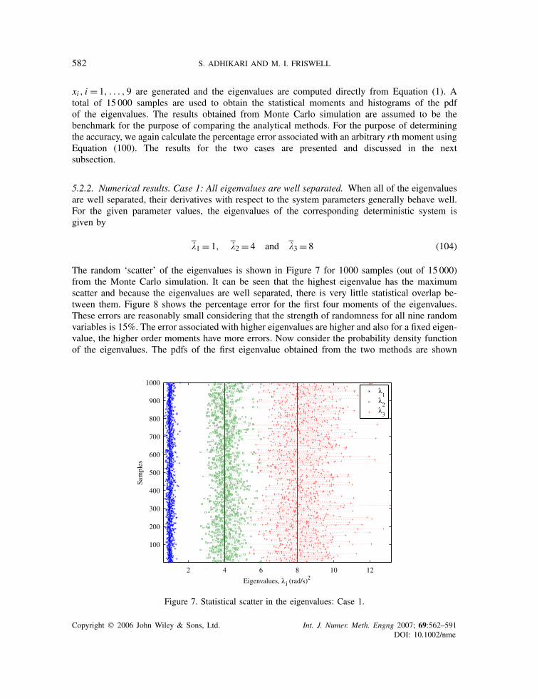
5.2.2. Numerical results. Case 1: All eigenvalues are well separated. When all of the eigenvaluesare well separated, their derivatives with respect to the system parameters generally behave well.For the given parameter values, the eigenvalues of the corresponding deterministic system isgiven by

�1 = 1, �2 = 4 and �3 = 8 (104)

The random ‘scatter’ of the eigenvalues is shown in Figure 7 for 1000 samples (out of 15 000)from the Monte Carlo simulation. It can be seen that the highest eigenvalue has the maximumscatter and because the eigenvalues are well separated, there is very little statistical overlap be-tween them. Figure 8 shows the percentage error for the first four moments of the eigenvalues.These errors are reasonably small considering that the strength of randomness for all nine randomvariables is 15%. The error associated with higher eigenvalues are higher and also for a fixed eigen-value, the higher order moments have more errors. Now consider the probability density functionof the eigenvalues. The pdfs of the first eigenvalue obtained from the two methods are shown

2 4 6 8 10 12

100

200

300

400

500

600

700

800

900

1000

Sam

ples

Eigenvalues, λj (rad/s)2

λ1

λ2

λ3

Figure 7. Statistical scatter in the eigenvalues: Case 1.



1 2 30

0.1

0.2

0.3

0.4

0.5

0.6

0.7

Eigenvalue number j

Perc

enta

ge e

rror

wrt

MC

S

First momentSecond momentThird momentFourth moment

Figure 8. Percentage error for first four moments of the eigenvalues: Case 1.

0.4 0.6 0.8 1 1.2 1.4 1.6 1.8 20

0.5

1

1.5

2

2.5

3

3.5

u

p λ 2(u)

Truncated Gaussian distributionχ2 distribution

Figure 9. Probability density function of the first eigenvalue: Case 1.

in Figure 9. On the same plot, normalized histograms of the eigenvalue obtained from the MonteCarlo simulation are also shown. Both approximate methods match well with the Monte Carlosimulation result. This is expected since the first three moments are obtained accurately (less



Figure 10. Probability density functions of the second and third eigenvalues: Case 1.

than 0.2% error as seen in Figure 8). The probability density functions of the second and thirdeigenvalues are shown in Figure 10. The region of statistical overlap is indeed small and can beverified from the plot of the actual samples in Figure 7. Again, both approximate methods matchwell with the Monte Carlo simulation result.

Case 2: Two eigenvalues are close. When some eigenvalues are closely spaced, their derivativeswith respect to the system parameters may not behave well [41]. Indeed, if repeated eigenvaluesexist, the formulation proposed here breaks down. The purpose of studying this case is to investigatehow the proposed methods work when there are closely spaced eigenvalues so that there is asignificant statistical overlap between them. For the given parameter values, the eigenvalues of thecorresponding deterministic system are calculated as

�1 = 1, �2 = 4 and �3 = 4.55 (105)

Clearly �2 and �3 are close to each other. The random scatter of the eigenvalues is shown inFigure 11 for 1000 samples from the Monte Carlo simulation. It can be seen that the thirdeigenvalue has the maximum scatter and because the second and the third eigenvalues are close,there is significant statistical overlap between them. Figure 12 shows the percentage error for thefirst four moments of the eigenvalues. The general trend of these errors are similar to the previouscase except that the magnitudes of the errors corresponding to second and third eigenvalues arehigher. This is expected because these two eigenvalues are close to each other.

The probability density function of the first eigenvalue obtained from the two methods areshown in Figure 13. On the same plot, normalized histograms of the eigenvalue obtained fromMonte Carlo simulation are also shown. As in the previous case, both approximate methods matchwell with the Monte Carlo simulation result. This is expected since the first three moments areobtained accurately for this case also. The probability density functions of the second and third



1 2 3 4 5 6 7 8

100

200

300

400

500

600

700

800

900

1000

Sam

ples

Eigenvalues, λ j (rad/s)2

λ1

λ2

λ3

Figure 11. Statistical scatter in the eigenvalues: Case 2.

1 2 30

0.5

1

1.5

2

2.5

Eigenvalue number j

Perc

enta

ge e

rror

wrt

MC

S

First momentSecond momentThird momentFourth moment

Figure 12. Percentage error for first four moments of the eigenvalues: Case 2.

eigenvalues are shown in Figure 14. There is a significant region of statistical overlap which canalso be verified from the plot of the actual samples in Figure 11. In this case, the truncated Gaussiandensity function performs better than the 2 density function. However, none of the approximatemethods match the Monte Carlo simulation result as well as in the previous case.



0.4 0.6 0.8 1 1.2 1.4 1.6 1.8 20

0.5

1

1.5

2

2.5

3

3.5

u

p λ 2(u)

Truncated Gaussian distributionχ2 distribution

Figure 13. Probability density function of the first eigenvalue: Case 2.

Figure 14. Probability density functions of the second and third eigenvalues: Case 2.

6. CONCLUSIONS

The statistics of the eigenvalues of discrete linear dynamic systems with parameter uncertaintieshave been considered. It is assumed that the mass and stiffness matrices are smooth and at least



twice differentiable functions of a set of random variables. The random variables are in generalconsidered to be non-Gaussian. The usual assumption of small randomness employed in mostmean-centred-based perturbation analysis is not employed in this study. Two methods, namely(a) optimal point expansion method, and (b) asymptotic moment method, are proposed. Theoptimal point is obtained so that the mean of the eigenvalues are estimated most accurately. Bothmethods are based on an unconstrained optimization problem. Moments and cumulants of arbitraryorders are derived for both the approaches. Two simple approximations for the probability densityfunction of the eigenvalues are derived. One is in terms of a truncated Gaussian random variableobtained using the maximum entropy principle. The other is a 2 random variable approximationbased on matching the first three moments of the eigenvalues. Both formulations yield closed-formexpressions of the pdf which can be computed easily.

The proposed formulae are applied to two problems. The moments and the pdf match en-couragingly well with the corresponding Monte Carlo simulation results. However, when someeigenvalues are closely spaced, the proposed methods do not produce very accurate results. Furtherresearch is required to deal with systems with closely spaced or repeated eigenvalues. In orderto obtain dynamic response statistics and system reliability, joint probability density functions ofthe eigenvalues and eigenvectors are required. Future studies will extend the proposed methods toobtain joint statistics of the eigenvalues.

APPENDIX A

A.1. Gradient vector and Hessian matrix of the eigenvalues

The eigenvectors of symmetric linear systems are orthogonal with respect to the mass and stiffnessmatrices. The eigenvectors are mass normalized, that is,

/TjM/ j = 1 (A1)

Using this and differentiating Equation (1) with respect to xk it can be shown that [42] for any x

�� j (x)

�xk=/ j (x)

TG jk(x)/ j (x) (A2)

where

G jk(x)=[�K(x)�xk

− � j (x)�M(x)�xk

](A3)

Differentiating Equation (1) with respect to xk , and xl , Plaut and Huseyin [43] have shown that,providing the eigenvalues are distinct,

�2� j (x)

�xk�xl=/ j (x)

T

[�2K(x)�xk�xl

− � j (x)�2M(x)�xk�xl

]/ j (x)

−(/ j (x)

T �M(x)�xk

/ j (x))(/ j (x)

TG jl(x)/ j (x))



−(/ j (x)

T �M(x)�xl

/ j (x))(/ j (x)

TG jk(x)/ j (x))

+ 2N∑

r=1

(/r (x)

TG jk(x)/ j (x))(/r (x)TG jl(x)/ j (x)

)� j (x) − �r (x)

(A4)

Equations (A2) and (A4) completely define the elements of the gradient vector and Hessian matrixof the eigenvalues.

A.2. Derivative of the system matrices with respect to the random variables

The derivatives of M(x) and K(x) with respect to elements of x can be obtained fromEquation (101) together with Equations (102) and (103). For the mass matrix we have

�M�x1

=⎡⎢⎣m1�m 0 0

0 0 0

0 0 0

⎤⎥⎦ ,�M�x2

=⎡⎢⎣0 0 0

0 m2�m 0

0 0 0

⎤⎥⎦ ,�M�x3

=⎡⎢⎣0 0 0

0 0 0

0 0 m3�m

⎤⎥⎦ (A5)

All other �M/�xi are null matrices. The derivatives of the stiffness matrix are

�K�x4

=

⎡⎢⎢⎣k1�k 0 0

0 0 0

0 0 0

⎤⎥⎥⎦ ,�K�x5

=

⎡⎢⎢⎣0 0 0

0 k2�k 0

0 0 0

⎤⎥⎥⎦ ,�M�x6

=

⎡⎢⎢⎣0 0 0

0 0 0

0 0 k3�k

⎤⎥⎥⎦�K�x7

=

⎡⎢⎢⎣k4�k −k4�k 0

−k4�k k4�k 0

0 0 0

⎤⎥⎥⎦ ,�K�x8

=

⎡⎢⎢⎣0 0 0

0 k5�k −k5�k

0 −k5�k k5�k

⎤⎥⎥⎦ ,�M�x9

=

⎡⎢⎢⎣k6�k 0 −k6�k

0 0 0

−k6�k 0 k6�k

⎤⎥⎥⎦(A6)

and all other �K/�xi are null matrices. Also note that all of the first-order derivative matrices areindependent of x. For this reason, all the higher order derivatives of the M(x) and K(x) matricesare null matrices.

APPENDIX B: NOMENCLATURE

a j constant in optimal perturbation expansionA j constant in optimal perturbation expansionc j constant in optimal perturbation expansiond(•)(x) gradient vector of (•) at xD(•)(x) Hessian matrix of (•) at x



E[•] mathematical expectation operatorI identity matrixK stiffness matrixL(x) negative of the log-likelihood functionm number of basic random variablesM� j (s) moment generating function of the eigenvaluesM mass matrixn number of moments used for pdf constructionN degrees-of-freedom of the systemO null matrixp(•) probability density function of (•)

x basic random variables

Greek letters

a optimal point for perturbation method�m, �k strength parameters associated with mass and stiffness coefficients j , � j , � j parameters of 2-approximated pdf of � j

h optimal point for asymptotic method�(r)j r th-order cumulant of the eigenvalues

� j eigenvalues of the systeml mean of parameter vector x�(r)j r th-order (raw) moment of the eigenvalues

�′(r)j r th-order central moment of the eigenvalues

�r Lagrange multipliers, r = 0, 1, 2, . . . , n� j standard deviation of � jR covariance matrix/ j eigenvectors of the system� cumulative Gaussian distribution function2� j (u) 2 density function with � j degrees-of-freedomL Lagrangian(•) deterministic value of (•)

(•)T matrix transpose≈ approximately equal toR space of real numbers‖•‖ determinant of matrix (•)

∈ belongs to�→ maps into| • | l2 norm of (•)

(•) mean of (•)

Abbreviations

dof degrees-of-freedomexp exponential functionpdf probability density function



ACKNOWLEDGEMENTS

S. Adhikari gratefully acknowledges the support of the Engineering and Physical Sciences ResearchCouncil through the award of an Advanced Research Fellowship. M. I. Friswell gratefully acknowledgesthe support of the Royal Society through a Royal Society-Wolfson Research Merit Award.

REFERENCES

1. Boyce WE. Random Eigenvalue Problems. Probabilistic Methods in Applied Mathematics. Academic Press:New York, 1968.

2. Scheidt JV, Purkert W. Random Eigenvalue Problems. North-Holland: New York, 1983.3. Ibrahim RA. Structural dynamics with parameter uncertainties. Applied Mechanics Reviews (ASME) 1987;

40(3):309–328.4. Benaroya H. Random eigenvalues, algebraic methods and structural dynamic models. Applied Mathematics and

Computation 1992; 52:37–66.5. Manohar CS, Ibrahim RA. Progress in structural dynamics with stochastic parameter variations: 1987 to 1998.

Applied Mechanics Reviews (ASME) 1999; 52(5):177–197.6. Manohar CS, Gupta S. Modeling and evaluation of structural reliability: current status and future directions. In

Research Reviews in Structural Engineering, Jagadish KS, Iyengar RN. (eds). Golden Jubilee Publications ofDepartment of Civil Engineering, Indian Institute of Science, Bangalore, University Press, 2003.

7. Collins JD, Thomson WT. The eigenvalue problem for structural systems with statistical properties. AIAA Journal1969; 7(4):642–648.

8. Hasselman TK, Hart GC. Modal analysis of random structural system. Journal of Engineering Mechanics (ASCE)1972; 98(EM3):561–579.

9. Hart GC. Eigenvalue uncertainties in stressed structure. Journal of Engineering Mechanics (ASCE) 1973;99(EM3):481–494.

10. Ramu SA, Ganesan R. Stability analysis of a stochastic column subjected to stochastically distributed loadingsusing the finite element method. Finite Elements in Analysis and Design 1992; 11:105–115.

11. Ramu SA, Ganesan R. Stability of stochastic Leipholz column with stochastic loading. Archive of AppliedMechanics 1992; 62:363–375.

12. Ramu SA, Ganesan R. A Galerkin finite element technique for stochastic field problems. Computer Methods inApplied Mechanics and Engineering 1993; 105:315–331.

13. Ramu SA, Ganesan R. Parametric instability of stochastic columns. International Journal of Solids and Structures1993; 30(10):1339–1354.

14. Sankar TS, Ramu SA, Ganesan R. Stochastic finite element analysis for high speed rotors. Transactions ofASME, Journal of Vibration and Acoustics 1993; 115:59–64.

15. Song D, Chen S, Qiu Z. Stochastic sensitivity analysis of eigenvalues and eigenvectors. Computers and Structures1995; 54(5):891–896.

16. den Nieuwenhof BV, Coyette JP. Modal approaches for the stochastic finite element analysis of structureswith material and geometric uncertainties. Computer Methods in Applied Mechanics and Engineering 2003;192(33–34):3705–3729.

17. Grigoriu M. A solution of random eigenvalue problem by crossing theory. Journal of Sound and Vibration 1992;158(1):69–80.

18. Lee C, Singh R. Analysis of discrete vibratory systems with parameter uncertainties, part I: Eigensolution.Journal of Sound and Vibration 1994; 174(3):379–394.

19. Nair PB, Keane AJ. An approximate solution scheme for the algebraic random eigenvalue problem. Journal ofSound and Vibration 2003; 260(1):45–65.

20. Hala M. Method of Ritz for random eigenvalue problems. Kybernetika 1994; 30(3):263–269.21. Mehlhose S, vom Scheidt J, Wunderlich R. Random eigenvalue problems for bending vibrations of beams.

Zeitschrift fur Angewandte Mathematik und Mechanik 1999; 79(10):693–702.22. Szekely GS, Schueller GI. Computational procedure for a fast calculation of eigenvectors and eigenvalues

of structures with random properties. Computer Methods in Applied Mechanics and Engineering 2001;191(8–10):799–816.

23. Pradlwarter HJ, Schueller GI, Szekely GS. Random eigenvalue problems for large systems. Computers andStructures 2002; 80(27–30):2415–2424.



24. Du S, Ellingwood BR, Cox JV. Initialization strategies in simulation-based SFE eigenvalue analysis. Computer-Aided Civil and Infrastructure Engineering 2005; 20(5):304–315.

25. Ghosh D, Ghanem RG, Red-Horse J. Analysis of eigenvalues and modal interaction of stochastic systems. AIAAJournal 2005; 43(10):2196–2201.

26. Adhikari S. Complex modes in stochastic systems. Advances in Vibration Engineering 2004; 3(1):1–11.27. Verhoosel CV, Gutierrez MA, Hulshoff SJ. Iterative solution of the random eigenvalue problem with application

to spectral stochastic finite element systems. International Journal for Numerical Methods in Engineering 2006,in press.

28. Rahman S. A solution of the random eigenvalue problem by a dimensional decomposition method. InternationalJournal for Numerical Methods in Engineering 2006, in press.

29. Mehta ML. Random Matrices (2nd edn). Academic Press: San Diego, CA, 1991.30. Muirhead RJ. Aspects of Multivariate Statistical Theory. Wiley: New York, U.S.A., 1982.31. Edelman A. Eigenvalues and condition numbers of random matrices. SIAM Journal on Matrix Analysis and

Applications 1988; 9:543–560.32. Dumitriu I, Edelman A. Matrix models for beta ensembles. Journal of Mathematical Physics 2002; 43:5830–5847.33. Johnson NL, Kotz S. Distributions in Statistics: Continuous Univariate Distributions—2. The Houghton Mifflin

Series in Statistics. Houghton Mifflin Company: Boston, U.S.A., 1970.34. Mathai AM, Provost SB. Quadratic Forms in Random Variables: Theory and Applications. Marcel Dekker:

New York, NY, 1992.35. Abramowitz M, Stegun IA. Handbook of Mathematical Functions, with Formulas, Graphs, and Mathematical

Tables. Dover Publications: New York, U.S.A., 1965.36. MacKay DJC. Information Theory, Inference and Learning Algorithms. Cambridge University Press: Cambridge,

MA, 2003.37. Bleistein N, Handelsman RA. Asymptotic Expansions of Integrals. Holt, Rinehart and Winston: New York, U.S.A.,

1994.38. Wong R. Asymptotic Approximations of Integrals. SIAM: Academic Press: Philadelphia, PA, U.S.A., 2001;

Academic Press, Inc.: Philadelphia, PA, U.S.A., 1989.39. Kapur JN, Kesavan HK. Entropy Optimization Principles With Applications. Academic Press: San Diego, CA,

1992.40. Pearson ES. Note on an approximation to the distribution of non-central 2. Biometrica 1959; 46:364.41. Friswell MI. The derivatives of repeated eigenvalues and their associated eigenvectors. Transactions of ASME,

Journal of Vibration and Acoustics 1996; 18:390–397.42. Fox RL, Kapoor MP. Rates of change of eigenvalues and eigenvectors. AIAA Journal 1968; 6(12):2426–2429.43. Plaut RH, Huseyin K. Derivative of eigenvalues and eigenvectors in non-self adjoint systems. AIAA Journal

1973; 11(2):250–251.


Documents

Randommatrixeigenvalueproblemsinstructuraldynamicsengweb.swan.ac.uk/~adhikaris/fulltext/journal/ft28.pdf · is based on a chi-square distribution. ... random eigenvalue problems;