Embed Size (px)
Citation preview

Randomized methods for matrix computations and analysis of high dimensional data
Per-Gunnar Martinsson
July 5, 2016.


Contents
Chapter 1. Matrix factorizations and low rank approximation 51.1. Notation, etc 51.2. Low rank approximation 61.3. The eigenvalue decomposition 71.4. The Singular Value Decomposition 71.5. The QR factorization 91.6. Subspaces associated with low rank approximation 14
Chapter 2. Randomized methods for low rank approximation 172.1. Introduction 172.2. A two-stage approach 172.3. A randomized algorithm for “Stage A” — the range finding problem 182.4. Single pass algorithms 192.5. A method with complexity O(mn log k) for dense matrices that fit in RAM 222.6. Theoretical performance bounds 232.7. An accuracy enhanced randomized scheme 242.8. The Nystrom method for positive symmetric definite matrices 262.9. Adaptive rank determination with updating of the matrix 272.10. Adaptive rank determination without updating the matrix 29
Chapter 3. Power iteration and Krylov methods 333.1. The basic power iteration 333.2. Subspace iteration 333.3. The general idea of Krylov methods 353.4. The Lanzcos algorithm 353.5. The Arnoldi process 393.6. A comparison of randomized methods and Krylov methods 403.7. Exercises 41
Chapter 4. Interpretation of data: The CUR and Interpolative Decompositions 434.1. The interpolative decomposition 434.2. Existence of the ID 444.3. Deterministic techniques for computing the ID 464.4. Computing interpolative decompositions via randomized sampling 474.5. The CUR Decomposition 494.6. Deterministic techniques for computing the CUR 514.7. Randomized techniques for computing the CUR 54
Bibliography 55


CHAPTER 1
Matrix factorizations and low rank approximation
The first chapter provides a quick review of basic concepts from linear algebra that we will use frequently. Note thatthe pace is fast here, and assumes that you have seen these concepts in prior course-work. If not, then additionalreading on the side is strongly recommended!
1.1. Notation, etc
1.1.1. Norms. Let x = [x1, x2, . . . , xn] denote a vector in Rn or Cn. Our default norm for vectors is theEuclidean norm
‖x‖ =
n∑j=1
|xj |21/2
.
We will at times also use `p norms
‖x‖p =
n∑j=1
|xj |p1/p
.
Let A denote an m×n matrix. For the most part, we allow A to have complex entries. We define the spectral normof A via
‖A‖ = sup‖x‖=1
‖Ax‖ = supx6=0
‖Ax‖‖x‖
.
We define the Frobenius norm of A via
‖A‖F =
m∑i=1
n∑j=1
|A(i, j)|21/2
.
Observe that‖A‖ ≤ ‖A‖F ≤
√min(m,n) ‖A‖.
1.1.2. Transpose and adjoint. Given an m×n matrix A, the transpose At is the n×m matrix B with entries
B(i, j) = A(j, i).
The transpose is most commonly used for real matrices. It can also be used for a complex matrix, but more typically,we then use the adjoint, which is the complex conjugate of the transpose
A∗ = At.
1.1.3. Subspaces. Let A be an m× n matrix.
• The row space of A is denoted row(A) and is defined as the subspace of Rn spanned by the rows of A.• The column space of A is denoted col(A) and is defined as the subspace of Rm spanned by the columns
of A. The column space is the same as the range or A, so col(A) = ran(A).• The nullspace or kernel of A is the subspace ker(A) = null(A) = x ∈ Rn : Ax = 0.

Randomized methods for matrix computations and data analysis P.G. Martinsson, July 5, 2016
1.1.4. Special classes of matrices. We use the following terminology to classify matrices:
• An m× n matrix A is orthonormal if its columns form an orthonormal basis, i.e. A∗A = I.• An n× n matrix A is normal if AA∗ = A∗A.• An n× n real matrix A is symmetric if At = A.• An n× n matrix A is self-adjoint if A∗ = A.• An n× n matrix A is skew-adjoint if A∗ = −A.• An n× n matrix A is unitary if it is invertible and A∗ = A−1.
Suppose that A is an n×n self-adjoint matrix. Then for any x ∈ Cn, one can easily verify that x∗Ax is a real scalarnumber. We then say that A is non-negative if x∗Ax ≥ 0 for all x ∈ Cn. The properties positive, non-positive, andnegative are defined analogously.
1.2. Low rank approximation
1.2.1. Exact rank deficiency. Let A be an m× n matrix. Let k denote an integer between 1 and min(m,n).Then the following conditions are equivalent:
• The columns of A span a subspace of Rm of dimension k.• The rows of A span a subspace of Rn of dimension k.• The nullspace of A has dimension n− k.• The nullspace of A∗ has dimension m− k.
If A satisfies any of these criteria, then we say that A has rank k. When A has rank k, it is possible to find matricesE and F such that
A = E F.m× n m× k k × n
The columns of E span the column space of A, and the rows of F span the row space of A. Having access to suchfactors E and F can be very helpful:
• Storing A requires mn words of storage.Storing E and F requires km+ kn words of storage.
• Given a vector x, computing Ax requires mn flops.Given a vector x, computing Ax = E(Fx) requires km+ kn flops.
• The factors E and F are often useful for data interpretation.
In practice, we often impose conditions on the factors. For instance, in the well known QR decomposition, thecolumns of E are orthonormal, and F is upper triangular (up to permutations of the columns).
1.2.2. Approximate rank deficiency. The condition that A has precisely rank k is of high theoretical interest,but is not realistic in practical computations. Frequently, the numbers we use have been measured by some devicewith finite precision, or they may have been computed via a simulation with some approximation errors (e.g. bysolving a PDE numerically). In any case, we almost always work with data that is stored in some finite precisionformat (typically about 10−15). For all these reasons, it is very useful to define the concept of approximate rank. Inthis course, we will typically use the following definition:
DEFINITION 1. Let A be an m × n matrix, and let ε be a positive real number. We then define the ε-rank of A asthe unique integer k such that both the following two conditions hold:
(a) There exists a matrix B of precise rank k such that ‖A− B‖ ≤ ε.(b) There does not exist any matrix B of rank less than k such that (a) holds
The term ε-rank is sometimes used without enforcing condition (b): We sometimes say that A has ε-rank k if
inf‖A− B‖ : B has rank k ≤ ε,6
Randomized methods for matrix computations and data analysis P.G. Martinsson, July 5, 2016
without worrying about whether the rank could actually be smaller. In other words, we sometimes say “A hasε-rank k” when we really mean “A has ε-rank at most k.”
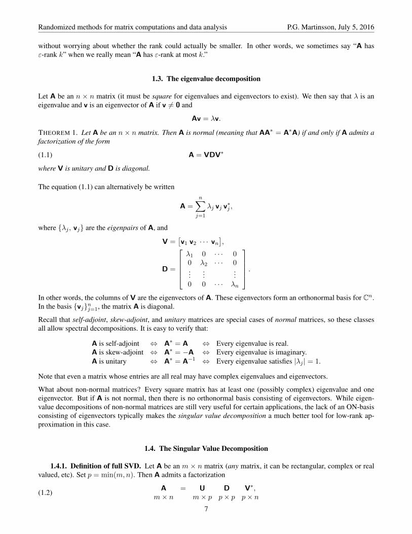
1.3. The eigenvalue decomposition
Let A be an n × n matrix (it must be square for eigenvalues and eigenvectors to exist). We then say that λ is aneigenvalue and v is an eigenvector of A if v 6= 0 and
Av = λv.
THEOREM 1. Let A be an n × n matrix. Then A is normal (meaning that AA∗ = A∗A) if and only if A admits afactorization of the form
(1.1) A = VDV∗
where V is unitary and D is diagonal.
The equation (1.1) can alternatively be written
A =n∑j=1
λj vj v∗j ,
where λj , vj are the eigenpairs of A, and
V =[v1 v2 · · · vn
],
D =
λ1 0 · · · 00 λ2 · · · 0...
......
0 0 · · · λn
.In other words, the columns of V are the eigenvectors of A. These eigenvectors form an orthonormal basis for Cn.In the basis vjnj=1, the matrix A is diagonal.
Recall that self-adjoint, skew-adjoint, and unitary matrices are special cases of normal matrices, so these classesall allow spectral decompositions. It is easy to verify that:
A is self-adjoint ⇔ A∗ = A ⇔ Every eigenvalue is real.A is skew-adjoint ⇔ A∗ = −A ⇔ Every eigenvalue is imaginary.A is unitary ⇔ A∗ = A−1 ⇔ Every eigenvalue satisfies |λj | = 1.
Note that even a matrix whose entries are all real may have complex eigenvalues and eigenvectors.
What about non-normal matrices? Every square matrix has at least one (possibly complex) eigenvalue and oneeigenvector. But if A is not normal, then there is no orthonormal basis consisting of eigenvectors. While eigen-value decompositions of non-normal matrices are still very useful for certain applications, the lack of an ON-basisconsisting of eigenvectors typically makes the singular value decomposition a much better tool for low-rank ap-proximation in this case.
1.4. The Singular Value Decomposition
1.4.1. Definition of full SVD. Let A be an m × n matrix (any matrix, it can be rectangular, complex or realvalued, etc). Set p = min(m,n). Then A admits a factorization
(1.2)A = U D V∗,
m× n m× p p× p p× n7

Randomized methods for matrix computations and data analysis P.G. Martinsson, July 5, 2016
where U and V are orthonormal, and where D is diagonal. We write these out as
U =[u1 u2 · · · up
],
V =[v1 v2 · · · vp
],
D =
σ1 0 · · · 00 σ2 · · · 0...
......
0 0 · · · σp
.The vectors ujpj=1 are the left singular vectors and the vectors vjpj=1 are the right singular vectors. Theseform orthonormal bases of the ranges of A and A∗, respectively. The values σjpj=1 are the singular values of A.These are customarily ordered so that
σ1 ≥ σ2 ≥ σ3 ≥ · · · ≥ σp ≥ 0.
The SVD (1.2) can alternatively be written as a decomposition of A as a sum of p “outer products” of vectors
A =
p∑j=1
σj uj v∗j .
1.4.2. Low rank approximation via SVD. For purposes of approximating a given matrix by a matrix of lowrank, the SVD is in a certain sense optimal. To be precise, suppose that we are given a matrix A, and have computedits SVD (1.2). Then for an integer k ∈ 1, 2, . . . , p, we define
Ak =
k∑j=1
σj uj v∗j .
Clearly Ak is a matrix of rank k. It is in fact the particular rank-k matrix that best approximates A:
‖A− Ak‖ = inf‖A− B‖ : B has rank k,‖A− Ak‖F = inf‖A− B‖F : B has rank k.
If k < p, then it is easily verified that the minimal residuals evaluate to
‖A− Ak‖ = σk+1,
‖A− Ak‖F =
p∑j=k+1
σ2j
1/2
.
REMARK 1.1. For normal matrices, a truncated eigenvalue decomposition attains exactly the same approximationerror as a truncated SVD, so for this particular class of matrices, either decomposition can be used. (But note thatthe EVD could be complex even for a real matrix.)
1.4.3. Connection between the SVD and the eigenvalue decomposition. Let A be a general matrix of sizem× n. Then form the m×m matrix
B = AA∗.
Observe that B is self-adjoint and non-negative, so there exist m orthonormal eigenvector ujmj=1 with associatedreal eigenvalues λjmj=1. Then ujmj=1 are left singular vectors of A associated with singular values σj =
√λj .
Analogously, if we form the n× n matrixC = A∗A,
then the eigenvectors of C are right singular vectors of A.
8

Randomized methods for matrix computations and data analysis P.G. Martinsson, July 5, 2016
1.4.4. Computing the SVD. One can prove that in general computing the singular values (or eigenvalues) ofan n× n matrix exactly is an equivalent problem to solving an n’th order polynomial (the characteristic equation).Since this problem is known to not, in general, have an algebraic solution for n ≥ 5, it is not surprising thatalgorithms for computing singular values are iterative in nature. However, they typically converge very fast, so forpractical purposes, algorithms for computing a full SVD perform quite similarly to algorithms for computing fullQR decompositions. For details, we refer to standard textbooks [7, 19], but some facts about these algorithms arerelevant to what follows:
• Standard algorithms for computing the SVD of a densem×nmatrix (as found in Matlab, LAPACK, etc),have practical asymptotic speed of O(mn min(m,n)).• While the asymptotic complexity of algorithms for computing full factorizations tend to beO(mn min(m,n))
regardless of the choice of factorization (LU, QR, SVD, etc), the scaling constants are different. In par-ticular pivoted QR is slower than non-pivoted QR, and the SVD is even slower.• Standard library functions for computing the SVD almost always produce results that are accurate to full
double precision accuracy. They can fail to converge for certain matrices, but in high-quality software,this happens very rarely.• Standard algorithms are challenging to parallelize well. For a small number of cores on a modern CPU
(as of 2016) they work well, but performance deteriorates as the number of cores increase, or if thecomputation is to be carried out on a GPU or a distributed memory machine.
1.5. The QR factorization
Let A be an m× n matrix. Set p = min(m,n). Let ajnj=1 denote the columns of A,
A =[a1 a2 · · · an
].
Our objective is now to find an orthonormal set of vectors qjpj=1 that form a “good” set of basis vectors for
expressing the columns of A. In other words, if we set
Qk =[q1 q2 · · · qk
],
then we want
‖A−QkQ∗kA‖ ≈ inf‖A− B‖ : B has rank k = σk+1.
We recall that the optimal basis (in this sense) is the left singular vectors of A. However, these are tricky to compute,and we seek a simpler and faster algorithm that leads to close to optimal basis vectors.
1.5.1. The Gram-Schmidt process. The Gram-Schmidt process is a simple “greedy” algorithm that can becoded efficiently. (Or at least reasonably efficiently, see Section 1.5.5.) Informally speaking, the idea is to takethe collection of vectors ajnj=1, grab the largest one, normalize it to make its length one, and then use theresulting vector as the first basis vector. Then project the remaining n− 1 vectors away from the one that was firstchosen. Then take the largest vector of the remaining ones, normalize it to form the second basis vector, project theremaining n− 2 vectors away from the new basis vector, etc. The resulting algorithm is shown in Figure 1.1.
REMARK 1.2 (Break-down for rank-deficient matrices). The process shown in Figure 1.1 will break down if thematrix has exact rank that is less than min(m,n). In this case, the residual matrix A will at some point be exactlyzero. For purposes of formulating a mathematically correct algorithm, all one needs to do is to introduce a stoppingcriterion that breaks the loop if this happens. In practice, since all computations are carried out in finite precision,the residual is very unlikely to ever be exactly zero. However, when the residual gets small, round-off errors willcreate serious loss of accuracy. Techniques that overcome this problem are described in Section 1.5.2.
9

Randomized methods for matrix computations and data analysis P.G. Martinsson, July 5, 2016
(1) Q0 = [ ]; R0 = [ ]; A0 = A; p = min(m,n);(2) for j = 1 : p
(3) ij = argmin‖A(:, `)‖ : ` = 1, 2, . . . , n(4) q = A(:, i)/‖A(:, i)‖.(5) r = q∗Aj−1
(6) Qj = [Qj−1 q]
(7) Rj =
[Rj−1
r
](8) Aj = Aj−1 − qr
(9) end for(10) Q = Qp; R = Rp;
FIGURE 1.1. The basic Gram Schmidt process. Given an input matrix A, the algorithm computesan ON matrix Q and a “morally” upper triangular matrix R such that A = QR. At the intermediatesteps, we have A = Aj + QjRj . Moreover at any step k, the columns of Q(:, 1 : k) form an ONbasis for the space spanned by the pivot vectors A(:, [i1, i2, . . . , ik]).
1.5.2. The QR factorization. Starting with the simplistic process described in Section (1.5.1), we will maketwo sets of improvements:
(1) Improving numerical accuracy: The method described in Figure 1.1 works perfectly when executed in ex-act arithmetic. However, for large matrices, the basis vectors generated tend to lose orthonormality as thecomputation proceeds. To avoid this, we perform an additional re-orthonormalization step. Specifically,after line (4), one should insert two new lines:
(4’) q = q−Qj−1 (Q∗j−1q).(4”) q = q/‖q‖.
These additional steps would make no difference in exact arithmetic, but they are important in practicalcomputations. Without them, you often lose orthonormality in the basis vectors, which greatly degradesthe utility of the computed factorization.
(2) Better pivoting: In practice, it is convenient to explicitly swap out the pivot vector you choose at step kto the k’th column in the matrix Q that you build. One must also do the analogous swap in the R matrixbeing built. (Moreover, it is possible to improve computational speed by accelerating the pivot selectionstep on line (3). The idea is to maintain a vector of length 1 × n that holds the sum of the squares ofall remaining residuals. This vector can be cheaply downdated at the end of the loop, which saves us theneed to compute the norms of the columns of Q. See [7, Sec. 5.4.1].)
(3) Improved book-keeping: The algorithm as written is wasteful of memory. One reasonably storage efficientway of implementing the method is to define at the outset a new matrix Q of sizem×n and simply copyingA over to Q. This matrix Q is used to hold both the new basis vectors that are stored in Qk in Figure 1.1and the residual columns that are stored in Ak in Figure 1.1. Observe that in each step, we zero out oneresidual vector, and create one new basis vector, so there is a perfect match. To be precise, at the end ofthe k’th step, the matrix Q holds Q =
[Qk Ak
], where Qk holds the computed k columns of Q, and Ak
holds the remaining n− k residual vectors.
The algorithm resulting from incorporating these improvements is given in Figure 1.2.
REMARK 1.3 (Householder QR). The QR factorization algorithm described in Figure 1.2 can be optimized further.In professional software packages, standard practice is to form the matrix Q as a product of so called Householderreflectors. These provide optimal stability and maintain very high orthonormality among the columns of Q. Further,when Householder reflectors are used, all the information needed to form R and Q can be stored in a single arrayof size m×n, as opposed to the formulation we give where two copies of the array are used. The trick is to use the
10

Randomized methods for matrix computations and data analysis P.G. Martinsson, July 5, 2016
Create and initialize the output matrices.(1) Q = A; R = zeros(min(m,n), n); J = 1 : n;(2) for j = 1 : min(m,n)
Find the pivot column i.(3) i = argmin‖Q(:, `)‖ : ` = j, j + 1, j + 2, . . . , n
Move the chosen pivot column to the j’th slot.(4) J([j, i]) = J([i, j]); Q(:, [j, i]) = Q(:, [i, j]); R(:, [j, i]) = R(:, [i, j]);(5) ρ = ‖Q(:, j)‖(6) R(j, j) = ρ
Perform the “paranoid” reorthonormalization.(7) q = (1/ρ) Q(:, j)
(8) q = q−Q(:, 1 : (j − 1)) (Q(:, 1 : (j − 1))∗ q)
(9) q = (1/‖q‖) q
(10) Q(:, j) = q
Compute the expansion coefficients and update Q and R.(11) r = q∗Q(:, (j + 1) : n)
(12) R(j, (j + 1) : n) = r
(13) Q(:, (j + 1) : n) = Q(:, (j + 1) : n)− qr
(14) end forIf n > m, then we need to delete the last columns of Q.
(15) Q = Q(:, 1 : min(m,n))
FIGURE 1.2. QR factorization via Gram Schmidt. The algorithm takes as input an m× n matrixA. The output is, with p = min(m,n), an index vector J , an m × p ON matrix Q, and a p × nupper triangular matrix R such that A(:, J) = QR.
zero elements formed “under the diagonal” in R to store enough information to uniquely define Q. See [7, Sec. 5.4]or [19, Lecture 10].
1.5.3. Low rank approximation via the QR factorization. The algorithm for computing the QR factoriza-tion can trivially be modified to compute a low rank approximation to a matrix. Consider the algorithm given inFigure 1.2. After k steps of the algorithm, we find that the matrices Q and R hold the following entries:
R =
[Rk
0
]and Q =
[Qk Ak
].
The matrix Rk is the matrix of size k×n holding the top k rows of R, the matrix Qk is of size m× k and holds thefirst k columns of Q, and the matrix Ak is of size m× (n− k) and holds the “remainder” of the columns that havenot yet been chosen as pivot columns (in other words, it contains the non-zero columns of the matrix Ak in Figure1.1). Then the partial factorization we have computed after k steps reads
(1.3) A(:, J) = QkRk +[0 Ak
].
Let Pk denote the permutation matrix defined by the index vector J so that
A(:, J) = APk.
Then we can rewrite (1.3) as (note that P−1k = P∗k)
A = QkRkP∗k +[0 Ak
]P∗k.
The first term has rank k and the second term is the “remainder.”
11
Randomized methods for matrix computations and data analysis P.G. Martinsson, July 5, 2016
Create and initialize the output matrices.(*) Q = A; R = zeros(min(m,n), n); J = 1 : n;(*) for j = 1 : min(m,n)
Find the pivot column i.(*) i = argmin‖Q(:, `)‖ : ` = j, j + 1, j + 2, . . . , n(*) J([j, i]) = J([i, j]); Q(:, [j, i]) = Q(:, [i, j]); R(:, [j, i]) = R(:, [i, j]);
Move the chosen pivot column to the j’th slot.(*) ρ = ‖Q(:, j)‖(*) R(j, j) = ρ
Perform the “paranoid” reorthonormalization.(*) q = (1/ρ) Q(:, j)
(*) q = q−Q(:, 1 : (j − 1)) (Q(:, 1 : (j − 1))∗ q)
(*) q = (1/‖q‖) q
(*) Q(:, j) = q
Compute the expansion coefficients and update Q and R.(*) r = q∗Q(:, (j + 1) : n)
(*) R(j, (j + 1) : n) = r
(*) Q(:, (j + 1) : n) = Q(:, (j + 1) : n)− qr
Check the accuracy of the partial factorization.if sum(sum(Q(:, (j + 1) : n). ∗Q(:, (j + 1) : n))) ≤ ε2 then break
(*) end for(*) k = j; Q = Q(:, 1 : k); R = R(1 : k, :);
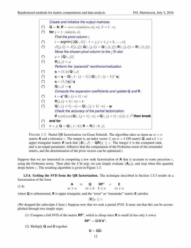
FIGURE 1.3. Partial QR factorization via Gram Schmidt. The algorithm takes as input an m× nmatrix A and a tolerance ε. The output is, an index vector J , an m× k ON matrix Q, and a k × nupper triangular matrix R such that ‖A(:, J) − QR‖F ≤ ε. The integer k is the computed rank,and is an output parameter. (Observe that the computation of the Frobenius norm of the remaindermatrix, and the determination of the pivot vectors can be optimized.)
Suppose that we are interested in computing a low rank factorization of A that is accurate to some precision ε,using the Frobenius norm. Then after the k’th step, we can simply evaluate ‖Ak‖F and stop when this quantitydrops below ε. The resulting algorithm is given in Figure 1.3.
1.5.4. Getting the SVD from the QR factorization. The technique described in Section 1.5.3 results in afactorization of the form
(1.4)A ≈ Q RP∗ + E
m× n m× k k × n m× nwhere Q is orthonormal, R is upper triangular, and the “error” or “remainder” matrix E satisfies
‖E‖F ≤ ε.(We dropped the subscripts k here.) Suppose now that we seek a partial SVD. It turns out that this can be accom-plished through two simple steps:
(1) Compute a full SVD of the matrix RP∗, which is cheap since R is small (it has only k rows)
RP∗ = U D V∗.
(2) Multiply Q and U togetherU = QU.
12

Randomized methods for matrix computations and data analysis P.G. Martinsson, July 5, 2016
Observe that now U and V are both orthonormal, D is diagonal, and
(1.5) A = Q RP∗︸︷︷︸=UDV∗
+E = QU︸︷︷︸=U
DV∗ + E = UDV∗ + E.
We have obtained a partial SVD. Observe in particular that the error term E is exactly the same in both (1.4) and(1.5).
1.5.5. Blocking of algorithms and execution speed. The various QR factorization algorithms described inthis section are extremely powerful and useful. They have been developed over decades, and current implemen-tations are highly accurate, entirely robust, and fairly fast. They suffer from one serious short coming, however,which is that they inherently are formed as a sequence of n low-rank updates to a matrix. The reason this is badis that on modern computers, the cost of moving data (from RAM to cache, between levels of cache, etc) oftenexceeds the time to execute flops. As an illustration of this phenomenon, suppose that we are given an m × nmatrix A and a set of vectors xipi=1, and that we seek to evaluate the vectors
yi = A xi, i = 1, 2, . . . , p.
One could either do this via a simple loop:
for i = 1 : p
yi = Axi
end for
Or, one could put all the vectors in a matrix and simply evaluate a matrix-matrix product:[y1 y2 · · · yp
]= A
[x1 x2 · · · xp
].
The two options are mathematically equivalent, and they both require precisely mnp flops. But, executing thecomputation as a matrix-matrix multiplication is much faster. To simplify slightly, the reason is that when youexecute the loop, the matrix A has to be read from memory p times. (Real life is more complicated since thecompiler might be smart and optimize the loop, etc.) In general, any linear algebraic operation that can be codedusing matrix-matrix operations tends to be much faster than a corresponding operation coded as a sequence ofmatrix-vector operators. Technically, we sometimes refer to “BLAS3” operations (matrix-matrix) versus “BLAS2”operations (martix-vector) [3, 1].
The problem with the column pivoted QR factorization is that it inherently consists of a sequence of BLAS2operations. This makes it hard to get good performance on multicore CPUs and GPUs (and in fact, even onsinglecore CPUs, due to the multiple levels of cache on modern processors). This leaves us in an uncomfortablespot when it comes to low rank approximation. To explain, suppose that A is an n× n matrix, and let us considerthree different matrix factorization algorithms:
(1) QR factorization without pivoting (“QR”).(2) QR factorization with column pivoting (“CPQR”).(3) Singular value decomposition (“SVD”).
All three algorithms have asymptotic complexity of O(n3), meaning that there are constants such that
TQR ∼ CQR n3, TCPQR ∼ CCPQR n
3, TSVD ∼ CSVD n3.
On most computer architectures we have CQR < CCPQR < CSVD, and the differences typically are not small.(See Exercise ??). Comparing these three algorithms, we find that:
Algorithm: QR CPQR SVDSpeed: Fast. Slow. Slowest.Ease of parallelization: Fairly easy. Very hard. Very hard.Useful for low-rank approximation: No. Yes. Excellent.Partial factorization possible? Yes, but not useful. Yes. Not easily.
13

Randomized methods for matrix computations and data analysis P.G. Martinsson, July 5, 2016
What we would want is an algorithm for low rank approximation that can be blocked so that it can be implementedusing BLAS3 operations rather than BLAS2 operations. It turns out that randomized sampling provides an excellentpath for this, as we will see in Section 2.
1.6. Subspaces associated with low rank approximation
This section briefly describes the geometric interpretation of low-rank approximation. Throughout the section,suppose that A is an m× n matrix of rank k. (Typically, this would be an approximate rank, but for simplicity, letus ignore the error for now.) Our starting point here is that we have computed rank k factorizations, either a QRfactorization
(1.6)A = Q R P∗
m× n m× k k × n n× n
or an SVD
(1.7)A = U D V∗.
m× n m× k k × k k × n
Set X = Rn and Y = Rm so that
A : X → Y.
Now observe that
(1.8) X = X1 ⊕X2, and Y = Y1 ⊕ Y2,
where
• X1 = row(A) is a subspace of rank k.• X2 = null(A) is a subspace of rank n− k.• Y1 = col(A) is a subspace of rank k.• Y2 = col(A)⊥ is a subspace of rank m− k.
The decomposition (1.8) clarifies the action of A. Given a vector x ∈ Rn, we write
x = x1︸︷︷︸∈X1
+ x2︸︷︷︸∈X2
.
Then Ax2 = 0, and so Ax = Ax1 + Ax2 = Ax1 ∈ Y1. So A maps X2 to zero, while the restriction A : X1 → Y1is one-to-one.
Next, let us discuss how the partial factorizations (1.6) and (1.7) provide us with bases for the fundamental spacesassociated with A:
The column space. This is easy, the columns of Q and U directly form ON-bases for col(A). The two basesare typically different.
The row space. If you have the SVD (1.7), then the columns of V form an ON-basis for row(A). If you havethe QR factorization (1.7), then the rows of R in principle form a basis for the row space of A, but it is not anorthonormal basis. Observe however that since k is small, it is easy to obtain an ON-basis by simply performingGram-Schmidt on the rows of RP∗ (pivoting is typically not required). For instance, if we execute[
S,∼]
= qr(PR∗, 0)
then the columns of S form an ON basis for row(A).
14

Randomized methods for matrix computations and data analysis P.G. Martinsson, July 5, 2016
The nullspace of a matrix. The partial factorizations we computed do not directly provide a basis for thenullspace of a matrix. If the matrix is small, then you could compute the full factorizations, and get the bases thatway. For big matrices, this tends to not be feasible, though. However, observe that the information provided isenough to characterize the null-space. Suppose that we have access to an n× k matrix V holding an ON basis forthe row space of A (e.g. the matrix of right singular vectors). Observe that we can then split the identity operator as
I = VV∗ +(I− VV∗
).
The first term is the orthogonal projection onto row(A), and the second term is the orthogonal projection ontorow(A)⊥ = null(A). In other words, given a vector x ∈ Rn, we can write
x = y + z,
where y and z are the orthogonal projections of x onto row(A) and null(A), respectively:
y = VV∗x ∈ row(A), and z = x− y =(I− VV∗
)x ∈ null(A).
15


CHAPTER 2
Randomized methods for low rank approximation
2.1. Introduction
This chapter describes randomized techniques for computing approximate low-rank factorizations to matrices. Toquickly introduce the key ideas, let us describe a simple prototypical randomized algorithm: Let A be a matrix ofsize m × n that is approximately of low rank. In other words, we assume that for some integer k < min(m,n),and some tolerance ε > 0, there exists a matrix Ak of rank k such that
‖A− Ak‖ ≤ ε.Then a natural question is how do you in a computationally efficient manner construct such a rank-k approximatingmatrix Ak? In 2006, it was observed in [13] (which was inspired by [6], and later led to [12, 14, 11]) that randommatrix theory provides a simple and elegant solution: Draw a Gaussian random matrix G of size n× k and form asampling matrix Y = AG. Then in many important situations, the matrix
(2.1) Ak := Y(Y†A
),
m× n m× k k × n
where Y† is the Moore-Penrose pseudo-inverse of Y, is close to optimal. With this observation as a starting point,one can construct highly efficient algorithms for computing approximate spectral decompositions of A, for solvingcertain least-squares problems, for doing principal component analysis of large data sets, etc.
Many of the randomized sampling techniques we will describe are supported by rigorous mathematical analysis.For instance, it has been proved that the matrix Ak defined by (2.1) provides almost as good of an approximationto A as the best possible approximant of rank, say, k − 5, with probability almost 1. (The number “5” in “k − 5”results from a particular choice of a tuning parameter.) See [11, Sec. 10] and Section 2.6.
The algorithms that result from using randomized sampling techniques are computationally efficient, and are sim-ple to implement as they rely on standard building blocks such as matrix-matrix multiplication, unpivoted QRfactorization, etc, that are available for most computing environments (multicore CPU, GPU, distributed memorymachines, etc). As an illustration, we invite the reader to peek ahead at Figure 2.1, which provides a completeMatlab code for a randomized algorithm that computes an approximate singular value decomposition of a matrix.Examples of improvements enabled by these randomized algorithms include:
• Given anm×nmatrix A, the cost of computing a rank-k approximant using classical methods isO(mnk).Randomized algorithms attain complexity O(mn log k + k2(m+ n)) [11, Sec. 6.1], and Section 2.5.• Techniques for performing principal component analysis (PCA) of large data sets have been greatly ac-
celerated, in particular when the data is stored out-of-core [10].• Randomized methods tend to require less communication than traditional methods, and can be efficiently
implemented on severely communication constrained environments such as GPUs [15] and even dis-tributed computing platforms such as the Amazon EC2 Cloud computer [9, Ch. 4].• Randomized algorithms enable single-pass matrix factorization in which the matrix is streamed and never
stored, cf. [11, Sec. 6.3] and Section 2.4.
2.2. A two-stage approach
The problem of computing an approximate low-rank factorization to a given matrix can conveniently be split intotwo distinct stages. For concreteness, we describe the split for the specific task of computing an approximate

Randomized methods for matrix computations and data analysis P.G. Martinsson, July 5, 2016
singular value decomposition. To be precise, given an m × n matrix A and a target rank k, we seek to computefactors U, D, and V such that
A ≈ U D V∗.m× n m× k k × k k × n
The factors U and V should be orthonormal, and D should be diagonal. (For now, we assume that the rank k isknown in advance, techniques for relaxing the assumption are described in Section 2.9.) Following [11], we splitthis task into two computational stages:
Stage A — find an approximate range: Construct anm×k matrix Q with orthonormal columns such thatA ≈ QQ∗A. This step will be executed via a randomized process described in Section 2.3.
Stage B — form a specific factorization: Given the matrix Q computed in Stage A, form factors U, D, andV, via classical deterministic techniques. For instance, this stage can be executed via the following steps:(1) Form the k × n matrix B = Q∗A.(2) Decompose the matrix B in a singular value decomposition B = UDV∗.(3) Form U = QU.
The point here is that in a situation where k min(m,n), the difficult part of the computation is concentrated toStage A. Once that is finished, the post-processing in Stage B is easy.
REMARK 2.1. Stage B is exact up to floating point arithmetic so all errors in the factorization process are incurredat Stage A. In other words, if the factor Q satisfies
||A−QQ∗A|| ≤ ε,then the full factorization satisfies
(2.2) ||A−UDV∗|| ≤ εunless ε is close to the machine precision. Note that (2.2) does not in general guarantee that the computed singularvectors in the matrices U and V are within distance ε of the exact leading k singular vectors. In many (but not all)contexts, this is not a problem since only the error in the product UDV∗ matters. (The computed singular valuesin D are within distance ε of the exact singular values, but note that for small singular values the relative precisionmay be poor.)
2.3. A randomized algorithm for “Stage A” — the range finding problem
This section describes a randomized technique for solving the range finding problem introduced as “Stage A” inSection 2.2. As a preparation for this discussion, let us recall that an “ideal” basis matrix Q for the range of a givenmatrix A is the matrix Uk formed by the k leading left singular vectors of A. Letting σj(A) denote the j’th singularvalue of B, the Eckard-Young theorem [18] states that
inf||A− C|| : C has rank k = ||A−UkV∗kA|| = σk+1(A).
Now consider a simplistic randomized method for constructing a spanning set with k vectors for the range of amatrix A: Draw k random vectors gjkj=1 from a Gaussian distribution, map these to vectors yj = Agj in therange of A, and then use the resulting set yjkj=1 as a basis. Upon orthonormalization via, e.g., Gram-Schmidt, anorthonormal basis qjkj=1 would be obtained. If the matrix A has exact rank k, then the vectors Agjkj=1 wouldwith probability 1 be linearly independent, and the resulting ON-basis qjkj=1 would exactly span the range of A.This would in a sense be an ideal algorithm. The problem is that in practice, there are almost always many non-zerosingular values beyond the first k ones. These modes will shift the sample vectors Agj out of the space spannedby the k leading singular vectors of A and the process described can (and frequently does) produce a poor basis.Luckily, there is a fix: Simple take a few extra samples. It turns out that if we take, say, k + 10 samples instead ofk, then the process will with probability almost 1 produce a basis that is comparable to the best possible basis.
To summarize the discussion in the previous paragraph, the randomized sampling algorithm for constructing anapproximate rank k basis for the range of a given m × n matrix A proceeds as follows: First pick a small integer
18

Randomized methods for matrix computations and data analysis P.G. Martinsson, July 5, 2016
ALGORITHM: RSVD — BASIC RANDOMIZED SVD
Inputs: An m× n matrix A, a target rank k, and an over-sampling parameter p (say p = 10).
Outputs: Matrices U, D, and V in an approximate rank-(k + p) SVD of A. (I.e. U and V are orthonormaland D is diagonal.)
Stage A:(1) Form an n× (k + p) Gaussian random matrix G. G = randn(n,k+p)(2) Form the sample matrix Y = A G. Y = A*G(3) Orthonormalize the columns of the sample matrix Q = orth(Y). [Q,∼] = qr(Y,0)
Stage B:(4) Form the (k + p)× n matrix B = Q∗A. B = Q’*A(5) Form the SVD of the small matrix B: B = UDV∗. [Uhat,D,V] = svd(B,’econ’)(6) Form U = QU. U = Q*Uhat
FIGURE 2.1. A basic randomized algorithm. If a factorization of precisely rank k is desired, thefactorization in Step 5 can be truncated to the k leading terms.
p representing how much “over-sampling” we do. (The choice p = 10 is often good.) Then execute the followingsteps:
(1) Form a set of k + p random Gaussian vectors gjk+pj=1 .
(2) Form a set yjk+pj=1 of samples from the range where yj = Agj .
(3) Perform Gram-Schmidt on the set yjk+pj=1 to form the ON-set qj
k+pj=1 .
Now observe that the k+pmatrix-vector products are independent and can advantageously be executed in parallel.A full algorithm for computing an approximate SVD using this simplistic sampling technique for executing “StageA” is summarized in Figure 2.1.
The error incurred by the randomized range finding method described in this section is a random variable. Thereexist rigorous bounds for both the expectation of this error, and for the likelihood of a large deviation from theexpectation. These bounds demonstrate that when the singular values of A decay “reasonably fast,” the errorincurred is close to the theoretically optimal one. We provide more details in Section 2.6.
2.4. Single pass algorithms
The randomized algorithm described in Figure 2.1 accesses the matrix A twice, first in “Stage A” where we build anON-basis for the column space, and then in “Stage B” where we project A on to the space spanned by the computedbasis vectors. It turns out to be possible to modify the algorithm in such a way that each entry of A is accessed onlyonce. This is important because it allows us to compute the factorization of a matrix that is too large to be storedeven out-of-core.
For Hermitian matrices, the modification to Algorithm 2.1 is very minor and we describe it in Section 2.4.1. Section2.4.2 then handles the case of a general matrix.
REMARK 2.2 (Loss of accuracy). The single-pass algorithms described in this section tend to produce a factoriza-tion of lower accuracy than what Algorithm 2.1 would yield. In situations where a two-pass algorithm is feasible,it is therefore often preferable to the single-pass algorithm.
REMARK 2.3 (Streaming Algorithms). We say that an algorithm for processing a matrix is a streaming algorithmif each entry of the matrix is accessed only once, and if, in addition, it can be fed the entries in any order. (Inother words, the algorithm is not allowed to dictate the order in which the elements are viewed.) The algorithmsdescribed in this section satisfy both of these conditions.
19

Randomized methods for matrix computations and data analysis P.G. Martinsson, July 5, 2016
2.4.1. Hermitian matrices. Suppose that A = A∗, and that our objective is to compute an approximateeigenvalue decomposition
(2.3)A ≈ U D U∗
n× n n× k k × k k × n
with U an ON matrix and D diagonal. (Note that for a Hermitian matrix, the EVD and the SVD are essentiallyequivalent, and that the EVD is the more natural factorization.) Then execute Stage A with an over-samplingparameter p to compute an ON matrix Q whose columns form an approximate basis for the column space of A:
(1) Draw a Gaussian random matrix G of size n× (k + p).(2) Form the sampling matrix Y = AG.(3) Orthonormalize the columns of Y to form Q, in other words Q = orth(Y).
Then
(2.4) A ≈ QQ∗A.
Observe that since in this case the column space and the row space are equivalent, we also have
(2.5) A ≈ AQQ∗.
Combine (2.4) and (2.5) to obtain
(2.6) A ≈ QQ∗AQQ∗.
We define
(2.7) C = Q∗AQ.
If C is known, then the post-processing is straight-forward: Simply compute the EVD of C to obtain C = UDU∗,
then define U = QU, to find thatA ≈ QCQ∗ = QUDU
∗Q∗ = UDU∗.
The problem now is that since we are seeking a single-pass algorithm, we are not in position to evaluate C directlyfrom formula (2.7). Instead, we will derive a formula for C that can be evaluated without revisiting A. To this end,multiply (2.7) by Q∗G to obtain
(2.8) C(Q∗G) = Q∗AQQ∗G ≈ Use (2.5) ≈ Q∗AG = Q∗Y
From (2.5), we know that AQQ∗ ≈ A so we can approximate right hand side in (2.8) via Q∗AQQ∗G ≈ Q∗AG =Q∗Y. Ignoring the approximation error, we define C as the solution of the linear system (recall ` = k + p)
(2.9) C(Q∗G
)=
(Q∗Y
).
`× ` `× ` `× `
At first, it may appears that (2.9) is perfectly balanced in that there are `2 equations for `2 unknowns. However, weneed to enforce that C is Hermitian, so the system is actually over-determined by roughly a factor of two.
The procedure described in this section is less accurate than the procedure described in Figure 2.1 for two reasons:
(1) The approximation error in formula (2.6) tends to be larger than the error in (2.4). In fact, with ε =‖A−QQ∗A‖, we have
‖A−QQ∗AQQ∗‖ = ‖A−QQ∗A‖+ ‖QQ∗A−QQ∗AQQ∗‖ =
ε+ ‖QQ∗(A− AQQ∗)‖ ≤ ε+ ‖A− AQQ∗‖ = 2ε,
where we used that ‖QQ∗‖ ≤ 1 (since Q is ON, and QQ∗ therefore is an ON projection) and that‖A − AQQ∗‖ = ‖(A − AQQ∗)∗‖ = ‖QQ∗A − A‖. In other words, we could in a worst case scenariodouble the error.
(2) While the matrix Q∗G is invertible, it tends to be very ill-conditioned.
20

Randomized methods for matrix computations and data analysis P.G. Martinsson, July 5, 2016
ALGORITHM: SINGLE-PASS RANDOMIZED EVD FOR A HERMITIAN MATRIX
Inputs: An n× n Hermitian matrix A, a target rank k, and an over-sampling parameter p (say p = 10).
Outputs: Matrices U and D in an approximate rank-k EVD of A. (I.e. U is orthonormal and D is diagonal.)
Stage A:(1) Form an n× (k + p) Gaussian random matrix G.(2) Form the sample matrix Y = A G.(3) Let Q denote the ON-matrix formed by the k dominant left singular vectors of Y.
Stage B:(4) Let C denote the k × k least squares solution of C
(Q∗G
)=(Q∗Y
)obtained by enforcing that C
should be Hermitian.(5) Decompose the matrix C in an eigenvalue decomposition [U, D] = eig(C).(6) Form U = QU.
FIGURE 2.2. A basic randomized algorithm single-pass algorithm suitable for a Hermitian matrix.
REMARK 2.4 (Extra over-sampling). The combat the problem that Q∗G tends to be ill-conditioned, it is helpful toover-sample more aggressively when using a single pass algorithm. Specifically, let us form Q as the leading k leftsingular vectors of Y (compute these by forming the full SVD of Y, and then discard the last p components). ThenC will be of size k × k, and the equation that specifies C reads
(2.10) C(QG)
= Q∗Y.k × k k × ` k × `
Since (2.10) is over-determined, we solve it using a least-squares technique. Observe that we are now looking forless information (a k × k matrix rather than an `× ` matrix), and have more information in order to determine it.
2.4.2. General matrices. Now consider a general m × n matrix A. We now need to apply randomized sam-pling to both its row space and its column space simultaneously. We proceed as follows:
(1) Draw two Gaussian random matrices Gc of size n× (k + p) and Gr of size m× (k + p).(2) Form two sampling matrices Yc = AGc and Yr = A∗Gr.(3) Compute two basis matrices Qc = orth(Yc) and Qr = orth(Yr).
Now define the small projected matrix via
(2.11) C = Q∗cAQr.
We will derive two relationships that together will determine C is a manner that is analogous to (2.8). First leftmultiply (2.11) by G∗rQc to obtain
(2.12) G∗rQcC = G∗rQcQ∗cAQr ≈ G∗rAQr = Y∗rQr.
Next we right multiply (2.11) by Q∗rGc to obtain
(2.13) CQ∗rGc = Q∗cAQrQ∗rGc ≈ Q∗cAGc = Q∗cYc.
We now define C as the least-square solution of the two equations(G∗rQc
)C = Y∗rQr and C
(Q∗rGc
)= Q∗cYc.
Again, the system is over-determined by about a factor of 2, and it is advantageous to make it further over-determined by more aggressive over-sampling, cf. Remark 2.4.
21

Randomized methods for matrix computations and data analysis P.G. Martinsson, July 5, 2016
ALGORITHM: SINGLE-PASS RANDOMIZED SVD FOR A GENERAL MATRIX
Inputs: An m× n matrix A, a target rank k, and an over-sampling parameter p (say p = 10).
Outputs: Matrices U, V, and D in an approximate rank-k SVD of A. (I.e. U and V are ON and D is diagonal.)
Stage A:(1) Form two Gaussian random matrices Gc = randn(n, k + p) and Gr = randn(m, k + p).(2) Form the sample matrices Yc = A Gc and Yr = A∗Gr.(3) Form ON matrices Qc and Qr consisting of the k dominant left singular vectors of Yc and Yr.
Stage B:(4) Let C denote the k×k least squares solution of the joint system of equations formed by the equations(
G∗rQc
)C = Y∗rQr and C
(Q∗rGc
)= Q∗cYc.
(5) Decompose the matrix C in a singular value decomposition [U, D, V] = svd(C).(6) Form U = QcU and V = QrV.
FIGURE 2.3. A basic randomized algorithm single-pass algorithm suitable for a general matrix.
2.5. A method with complexity O(mn log k) for dense matrices that fit in RAM
The RSVD algorithm described in Figure 2.1 for constructing an approximate basis for the range of a given matrixA is highly efficient when we have access to fast algorithms for evaluating matrix-vector products x 7→ Ax. For thecase where A is a general m×n matrix given simply as an array or real numbers, the cost of evaluating the samplematrix Y = AG (in Step (2) of the algorithm in Figure 2.1) is O(mnk). The algorithm is still often faster thanclassical methods since the matrix-matrix multiply can be highly optimized, but it does not have an edge in termsof asymptotic complexity. However, it turns out to be possible to modify the algorithm by replacing the Gaussianrandom matrix G with a different random matrix Ω that has two seemingly contradictory properties:
(1) Ω is sufficiently structured that the product AΩ can be evaluated in O(mn log(k)) flops.(2) Ω is sufficiently random that the columns of AΩ accurately span the range of A.
For instance, a good choice Ω is
(2.14)Ω = D F S,
n× ` n× n n× n n× `where D is a diagonal matrix whose diagonal entries are complex numbers of modulus one drawn from a uniformdistribution on the unit circle in the complex plane, where F is the discrete Fourier transform,
F(p, q) = n−1/2 e−2πi(p−1)(q−1)/n, p, q ∈ 1, 2, 3, . . . , n,
and where S is matrix consisting of a random subset of ` columns from the n × n unit matrix (drawn withoutreplacement). In other words, given an arbitrary matrix X of size m × n, the matrix XS consists of a randomlydrawn subset of ` columns of X. For the matrix Ω specified by (2.14), the product XΩ can be evaluated via asubsampled FFT in O(mn log(`)) operations. The parameter ` should be chosen slightly larger than the target rankk; the choice ` = 2k is often good.
By using the structured random matrix described in this section, we can reduce the complexity of “Stage A” in theRSVD from O(mnk) to O(mn log k). We next need to modify “Stage B” to eliminate the need to compute Q∗A.One option is to use the single pass algorithm described in 2.3, using the structured random matrix to approximateboth the row and the column spaces of A. A second, and typically better, option is to use a so called row-extractiontechnique for Stage B, we describe the details in Section 4.4.
The current error analysis for the accelerated range finder is less satisfactory than the one for Gaussian randommatrices. In the general case, only very weak results can be proven. In practice, the accelerated scheme is often asaccurate as the Gaussian one, but we do not currently have good theory to predict precisely when this happens, see[11, Sec. 11].
22

Randomized methods for matrix computations and data analysis P.G. Martinsson, July 5, 2016
2.6. Theoretical performance bounds
In this section, we will briefly summarize some proven results concerning the error in the output of the basic RSVDalgorithm in Figure 2.1. Observe that the factors U, D, V depend not only on A, but also on the draw of the randommatrix G. This means that the error that we try to bound is a random variable. It is therefore natural to seek boundson first the “expectation” or “mean” of the error, and then on the likelihood of large deviations from the mean.
Before we start, let us recall that all the error incurred by the RSVD algorithm in Figure 2.1 is incurred in Stage A.The reason is that the “post-processing” in Stage B is exact (up to floating point arithmetic):
A−Q Q∗A︸︷︷︸=B
= A−Q B︸︷︷︸=UDV∗
= A− QU︸︷︷︸=U
DV∗ = A−UDV∗.
Consequently, we can (and will) restrict ourselves to providing bounds on ‖A−QQ∗A‖.
2.6.1. Bounds on the expectation of the error. For instance, Theorem 10.6 of [11] states:
THEOREM 2. Let A be an m × n matrix with singular values σjmin(m,n)j=1 . Let k be a target rank, and let p be
an over-sampling parameter such that p ≥ 2 and k + p ≤ min(m,n). Let G be a Gaussian random matrix of sizen× (k + p) and set Q = orth(AG). Then the average error, as measured in the Frobenius norm, satisfies
(2.15) E[‖A−QQ∗A‖Fro
]≤(
1 +k
p− 1
)1/2min(m,n)∑
j=k+1
σ2j
1/2
.
The corresponding result for the spectral norm reads
(2.16) R[‖A−QQ∗A‖
]≤
(1 +
√k
p− 1
)σk+1 +
e√k + p
p
min(m,n)∑j=k+1
σ2j
1/2
.
When errors are measured in the Frobenius norm, Theorem 2 is very gratifying. For our standard recommendationof p = 10, we are basically within a factor of
√k/10 of the theoretically minimal error. (Recall that the Eckart-
Young theorem states that(∑min(m,n)
j=k+1 σ2j
)1/2is a lower bound on the residual for any rank-k approximant.) If
you over-sample a little more aggressively and set p = k, then we are within a distance of√
2 of the theoreticallyminimal error.
When errors are measured in the spectral norm, the situation is much less rosy. The first term in the bound in (2.16)is perfectly acceptable, but the second term is unfortunate in that it involves the minimal error in the Frobeniusnorm, which can be a much bigger factor and potentially renders this bound highly sub-optimal. The theorem isquite sharp, as it turns out, so this disparity reflects a true problem for the basic randomized scheme.
The extent to which the suboptimality in (2.16) is problematic depends on how rapidly the “tail” singular valuesσjj>k decay. If they decay fast, then the spectral norm error and the Frobenius norm error are similar, and theRSVD works well. If they decay slowly, then the RSVD performs OK when errors are measured in the Frobeniusnorm, but not very well when the spectral norm is the one of interest. To illustrate the difference, let us considertwo situations:
Case 1 — fast decay: Suppose that the tail singular values decay exponentially fast, so that for some β ∈ (0, 1)
we have σj ≈ σk+1 βj−k−1 for j > k. Then
(∑min(m,n)j=k+1 σ2j
)1/2≈ σk+1
(∑min(m,n)j=k+1 β2
)1/2≤ σk+1(1 −
β2)−1/2. As long as β is not very close to 1, we see that the contribution from the tail singular values is verymodest in this case.
Case 2 — no decay: Suppose that the tail singular values exhibit no decay, so that σj = σk+1 for j > k. This
represents the worst case scenario, and now(∑min(m,n)
j=k+1 σ2j
)1/2= σk+1
√n− k. Since we want to allow for n
to be very large (say n = 106), this represents a huge degree of suboptimality.
23

Randomized methods for matrix computations and data analysis P.G. Martinsson, July 5, 2016
Fortunately, it is possible to modify the RSVD in such a way that the errors produced are close to optimal in boththe spectral and the Frobenius norms. This is achieved by modestly increasing the computational cost. See Section2.7 and [11, Sec. 4.5].
2.6.2. Bounds on the likelihood of large deviations. One can prove that (perhaps surprisingly) the likelihoodof a large deviation from the mean depends only on the over-sampling parameter p, and decays extra-ordinarily fast.For instance, one can prove that if p ≥ 4, then
(2.17) ||A−QQ∗A|| ≤(
1 + 17√
1 + k/p)σk+1 +
8√k + p
p+ 1
(∑j>k
σ2j
)1/2,
with failure probability at most 3 e−p, see [11, Cor. 10.9].
2.7. An accuracy enhanced randomized scheme
2.7.1. The key idea — power iteration. We mentioned earlier that the basic randomized scheme (see, e.g.,Figure 2.1) gives accurate results for matrices whose singular values decay rapidly, but tends to produce suboptimalresults when they do not. The theoretical results summarized in Section 2.6 make this claim precise. To recap,suppose that we compute a rank-k approximation to an m × n matrix A with singular values σjj . The theoryshows that the error measured in the spectral norm behaves like
(∑j>k σ
2j
)1/2. When the singular values decayslowly, this quantity can be much larger than the theoretically minimal approximation error (which is σk+1).
Recall that the objective of the randomized sampling is to construct a set of ON vectors qj`j=1 that capture tohigh accuracy the space spanned by the k dominant left singular vectors ujkj=1 of A. The idea is now to samplenot A, but the matrix
A(q) :=(AA∗
)qA,
where q is a small positive integer (typically, q = 1 or q = 2). A simple calculation shows that if A has singularvalue decomposition A = UDV∗, then the SVD of A(q) is
A(q) = U D2q+1 V∗.
In other words, A(q) has the same left singular values as A, while its singular values are σ2q+1j j . Even when the
singular values of A decay slowly, the singular values of A(q) tend to decay fast enough for our purposes.
The accuracy enhanced scheme now consists of drawing a Gaussian matrix G and then forming a sample matrix
Y =(AA∗
)qAG.
Then orthonormalize the columns of Y to obtain Q = orth(Y), and proceed as before. The resulting scheme isshown in Figure 2.4.
REMARK 2.5. The scheme described in Figure 2.4 can lose accuracy due to round-off errors. The problem is thatas q increases, all columns in the sample matrix Y =
(AA∗
)qAG tend to align closer and closer to the dominant
left singular vector. This means that we lose almost all accuracy in regards to the directions of singular valuesassociated with smaller singular vectors. Roughly speaking, if
σjσ1≤ ε1/(2q+1)
mach ,
then all information associated with the j’th singular more is lost. This issue is explored in more detail in Section3.2. For now, let us simply state a variation of the scheme in Figure 2.4 that ameliorates the round-off error problemby explicitly orthonormalizing the sample vectors between each iteration:
24

Randomized methods for matrix computations and data analysis P.G. Martinsson, July 5, 2016
ALGORITHM: ACCURACY ENHANCED RANDOMIZED SVD
Inputs: An m× n matrix A, a target rank k, an over-sampling parameter p (say p = 10), and a small integerq denoting the number of steps in the power iteration.
Outputs: Matrices U, D, and V in an approximate rank-(k + p) SVD of A. (I.e. U and V are orthonormaland D is diagonal.)
(1) G = randn(n, k + p);(2) Y = AG;(3) for j = 1 : q
(4) Z = A∗Y;
(5) Y = AZ;
(6) end for(7) Q = orth(Y);(8) B = Q∗A;
(9) [U, D, V] = svd(B,’econ’);
(10) U = QU;
FIGURE 2.4. The accuracy enhanced randomized SVD. If a factorization of precisely rank k isdesired, the factorization in Step 5 can be truncated to the k leading terms.
(1) G = randn(n, k + p);(2) Q = orth(AG);(3) for j = 1 : q
(4) W = orth(A∗Q);
(5) Q = orth(AW);
(6) end for(7) B = Q∗A;
(8) [U, D, V] = svd(B,’econ’);
(9) U = QU;
This scheme is more costly due to the calls to orth. However, this orthonormalization can be executed usingunpivoted Gram-Schmidt, which is quite fast.
2.7.2. Theoretical results. A detailed error analysis of the scheme described in Figure 2.4 is provided in [11,Sec. 10.4]. In particular, the key theorem states the following:
THEOREM 3. Let A denote an m × n matrix, let p ≥ 2 be an over-sampling parameter, and let q denote a smallinteger. Draw a Gaussian matrix G of size n× (k+ p), set Y = (AA∗)qAG, and let Q denote an m× (k+ p) ONmatrix resulting from orthonormalizing the columns of Y. Then
(2.18) E[‖A−QQ∗A‖
]≤
[(1 +
√k
p− 1
)σ2q+1k+1 +
e√k + p
p
(∑j>k
σ2(2q+1)j
)1/2]1/(2q+1)
.
The bound in (2.18) is slightly hard to decipher. To simplify it, let us consider the worst case scenario where thereis no decay in the singular values beyond the truncation point, so that σk+1 = σk+2 = · · · = σmin(m,n). Then(2.18) simplifies to
E[‖A−QQ∗A‖
]≤
[1 +
√k
p− 1+e√k + p
p·√
minm,n − k
]1/(2q+1)
σk+1.
25
Randomized methods for matrix computations and data analysis P.G. Martinsson, July 5, 2016
In other words, as we increase the exponent q, the power scheme drives factor set in blue to one exponentially fast.This factor represents the degree of “sub-optimality” you can expect to see.
2.7.3. Extended sampling matrix. The scheme described in Section 2.7.1 is slightly wasteful in that it doesnot directly use all the sampling vectors computed. To further improve accuracy, let us form an “extended” samplingmatrix
Y =[AG, A2G, . . . , AqG
].
Observe that this new sampling matrix Y has q` columns. Then proceed as before:
Q = qr(Y), B = Q∗A, [U,D,V] = svd(B,’econ’), U = QU.
Note that these computations are all much more expensive than those in Section 2.7.1 since we now work with ma-trices with q` columns, as opposed to ` columns earlier. Since the cost of QR factorization, etc, grows quadraticallywith the number of columns, the difference is very substantial — the cost of dense linear algebra increases by afactor of O(q2). Consequently, the scheme described here is primarily useful in situations where the computationalcost is dominated by applications of A and A∗, and we want to maximally leverage all interactions with A.
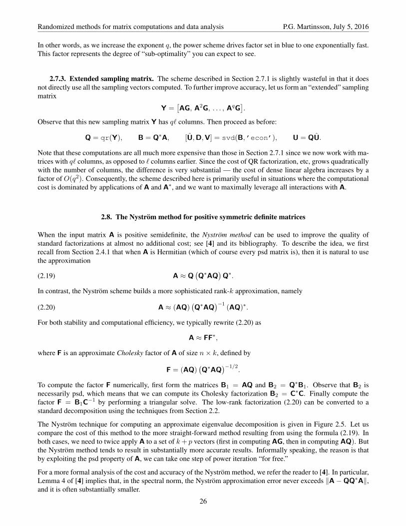
2.8. The Nystrom method for positive symmetric definite matrices
When the input matrix A is positive semidefinite, the Nystrom method can be used to improve the quality ofstandard factorizations at almost no additional cost; see [4] and its bibliography. To describe the idea, we firstrecall from Section 2.4.1 that when A is Hermitian (which of course every psd matrix is), then it is natural to usethe approximation
(2.19) A ≈ Q(Q∗AQ
)Q∗.
In contrast, the Nystrom scheme builds a more sophisticated rank-k approximation, namely
(2.20) A ≈ (AQ)(Q∗AQ
)−1(AQ)∗.
For both stability and computational efficiency, we typically rewrite (2.20) as
A ≈ FF∗,
where F is an approximate Cholesky factor of A of size n× k, defined by
F = (AQ)(Q∗AQ
)−1/2.
To compute the factor F numerically, first form the matrices B1 = AQ and B2 = Q∗B1. Observe that B2 isnecessarily psd, which means that we can compute its Cholesky factorization B2 = C∗C. Finally compute thefactor F = B1C−1 by performing a triangular solve. The low-rank factorization (2.20) can be converted to astandard decomposition using the techniques from Section 2.2.
The Nystrom technique for computing an approximate eigenvalue decomposition is given in Figure 2.5. Let uscompare the cost of this method to the more straight-forward method resulting from using the formula (2.19). Inboth cases, we need to twice apply A to a set of k+ p vectors (first in computing AG, then in computing AQ). Butthe Nystrom method tends to result in substantially more accurate results. Informally speaking, the reason is thatby exploiting the psd property of A, we can take one step of power iteration “for free.”
For a more formal analysis of the cost and accuracy of the Nystrom method, we refer the reader to [4]. In particular,Lemma 4 of [4] implies that, in the spectral norm, the Nystrom approximation error never exceeds ‖A−QQ∗A‖,and it is often substantially smaller.
26

Randomized methods for matrix computations and data analysis P.G. Martinsson, July 5, 2016
ALGORITHM: EIGENVALUE DECOMPOSITION VIA THE NYSTROM METHOD
Given an n×n non-negative matrix A, a target rank k and an over-sampling parameter p, this procedurecomputes an approximate eigenvalue decomposition A ≈ UΛU∗, where U is orthonormal, and Λ isnonnegative and diagonal.
(1) Draw a Gaussian random matrix G = randn(n, k + p).(2) Form the sample matrix Y = AG.(3) Orthonormalize the columns of the sample matrix to obtain the basis matrix Q = orth(Y).(4) Form the matrices B1 = AQ and B2 = Q∗B1.(5) Perform a Cholesky factorization B2 = C∗C.(6) Form F = B1C−1 using a triangular solve.(7) Compute an SVD of the Cholesky factor [U, Σ,∼] = svd(F,’econ’).(8) Set Λ = Σ2.
FIGURE 2.5. The Nystrom method. This procedure is applicable only to self-adjoint matriceswith non-negative eigenvalues. It involves two applications of A to matrices with k columns,and consequently has comparable cost to the basic RSVD in Figure 2.1. However, it exploits thesymmetry of A to boost the accuracy.
2.9. Adaptive rank determination with updating of the matrix
2.9.1. Problem formulation. Up to this point, we have assumed that the rank k is given as an input vari-able to the factorization algorithm. In practical usage, it is common that we are given instead a matrix A and acomputational tolerance ε, and our task is then to determine a matrix Bk of rank k such that ‖A− Bk‖ ≤ ε.
The techniques described in this section are designed for dense matrices stored in RAM. They directly updatethe matrix, and come with a firm guarantee that the computed low rank approximation is within distance ε of theoriginal matrix. There are many situations where direct updating is not feasible and we can in practice only interactwith the matrix via the matrix-vector multiplication (e.g., very large matrices stored out-of-core, sparse matrices,matrices that are defined implicitly). Section 2.10 describes algorithms designed for this environment that userandomized sampling techniques to estimate to approximation error.
Recall that for the case where a computational tolerance is given (rather than a rank), the optimal solution isgiven by the SVD. Specifically, let σjmin(m,n)
k=1 be the singular values of A. Then the minimal rank k for whichinf‖A − B‖ : B has rank k is the smallest integer k such that σk+1 ≤ ε. The algorithms described here willdetermine a k that is not necessarily optimal, but is typically fairly close.
2.9.2. A basic updating algorithm. Let us start by describing a very general algorithmic template for howto compute an approximate rank-k approximate factorization of a matrix. To be precise, suppose that we aregiven an m × n matrix A, and a computational tolerance ε. Our objective is then to determine an integer k ∈1, 2, . . . ,min(m,n), an m× k ON matrix Qk, and a k × n matrix Bk such that
‖ A − Qk Bk ‖ ≤ ε.m× n m× k k × n
This problem can be solved using the greedy algorithm shown in Figure 2.6 which builds Qk and Bk one columnand row at a time.
The algorithm described in Figure 2.6 is a generalization of the basic Gram-Schmidt procedure described in Figure1.1. The key to understanding how the algorithm works is provided by the identity
A = QjBj + Aj , j = 0, 1, 2, . . . , k.
The computational efficiency and accuracy of the algorithm depends crucially on how the vector y is picked on line(4). Let us consider three possible selection strategies:
27

Randomized methods for matrix computations and data analysis P.G. Martinsson, July 5, 2016
(1) Q0 = [ ]; B0 = [ ]; A0 = A; k = 0;(2) while ‖Ak‖ > ε
(3) k = k + 1
(4) Pick a vector y ∈ Ran(Ak−1)
(5) q = y/‖y‖.(6) b = q∗Ak−1
(7) Qk = [Qk−1 q]
(8) Bk =
[Bk−1
b
](9) Ak = Ak−1 − qb
(10) end for
FIGURE 2.6. A greedy algorithm for building a low-rank approximation to a given m× n matrixA that is accurate to within a given precision ε. To be precise, the algorithm determines an integerk, an m× k ON matrix Qk and a k × n matrix Bk = Q∗kA such that ‖A−QkBk‖ ≤ ε. One caneasily verify that after the algorithm finishes, we have A = QjBj + Aj for any j = 0, 1, 2, . . . , k.
Pick the largest remaining column. Suppose we instantiate line (4) by letting y be simply the largest columnof the remainder matrix Ak−1.
(4) Set jk = argmax‖Ak−1(:, j)‖ : j = 1, 2, . . . , n and then y = Ak−1(:, jk).
With this choice, the algorithm in Figure 2.6 is precisely column pivoted Gram-Schmidt (CPQR). This algorithmis reasonably efficient, and often leads to fairly close to optimal low-rank approximation. For instance, when thesingular values of A decay rapidly, CPQR typically determines a numerical rank k that is typically reasonably closeto the theoretically exact ε-rank. However, this is not always the case even when the singular values decay rapidly,and the results can be quite poor when the singular values decay slowly.
Pick the locally optimal vector. A choice that is natural, and is conceptually very simple is to pick the vector yby solving the obvious minimization problem:
(4) y = argmin‖Ak−1 − yy∗Ak−1‖ : ‖y‖ = 1.
With this choice, the algorithm will produce matrices that attain the theoretically optimal precision
‖A−QjBj‖ = σj+1.
This tells us that the greediness of the algorithm is not a problem. However, solving the local minimization problemis sufficiently computationally hard that this algorithm is not particularly practical.
A randomized selection strategy. Suppose now that we pick y by forming a linear combination of the columnsof Ak−1 with the expansion weights drawn from a normalized Gaussian distribution:
(4) Draw a Gaussian random vector g ∈ Rn and set y = Ak−1g.
With this choice, the algorithm becomes logically equivalent to the basic randomized SVD given in Figure 2.1. Thismeans that this choice often leads to a factorization that is close to optimally accurate, and is also computationallyefficient. One can attain higher accuracy by trading away some computational efficiency by incorporating a coupleof steps of power iteration, and choosing y =
(Ak−1A∗k−1
)qAk−1g for some small integer q.
2.9.3. A blocked updating algorithm. A key benefit of the randomized greedy algorithm described in Section2.9.2 is that it can easily be blocked. In other words, given a block size `, we can at each step of the iteration drawa set of ` Gaussian random vectors, compute the corresponding sample vectors, and then extend the factors Q andB by adding ` columns and ` rows at a time, respectively. The resulting algorithm is shown in Figure 2.7.
28

Randomized methods for matrix computations and data analysis P.G. Martinsson, July 5, 2016
(1) Q = [ ]; B = [ ];(2) while ‖A‖ > ε
(3) Draw an n× ` random matrix R.(4) Compute the m× ` matrix Qnew = qr(AR, 0).(5) Bnew = Q∗newA
(6) Q = [Q Qnew]
(7) B =
[B
Bnew
](8) A = A−QnewBnew
(9) end while
FIGURE 2.7. A greedy algorithm for building a low-rank approximation to a given m× n matrixA that is accurate to within a given precision ε. This algorithm is a blocked analogue of the methoddescribed in Figure 2.6 and takes as input a block size `. Its output is an ON matrix Q of sizem×k(where k is a multiple of `) and a k × n matrix B such that ‖A−QB‖ ≤ ε. For higher accuracy,one can incorporate a couple of steps of power iteration and set Qnew = qr((AA∗)qAR, 0) onLine (4).
(1) Q0 = [ ]; B0 = [ ];(2) for j = 1, 2, 3, . . .
(3) Draw a Gaussian random vector gj ∈ Rn and set yj = Agj(4) Set zj = yj −Qj−1Q∗j−1yj and then qj = zj/|zj |.(5) Qj = [Qj−1 qj ]
(6) Bj =
[Bj−1q∗jA
](7) end for
FIGURE 2.8. A randomized range finder that builds an ON-basis q1,q2,q3, . . . for the rangeof A one vector at a time. This algorithm is mathematically equivalent to the basic RSVD inFigure 2.1 in the sense that if G = [g1 g2 g3 . . . ], then the vectors qj
pj=1 form an ON-basis for
AG(:, 1 : p) for both methods. Observe that zj =(A−Qj−1Q∗j−1A
)gj , cf. (2.21).
2.10. Adaptive rank determination without updating the matrix
The techniques described in Section 2.9 for computing a low rank approximation to a matrix A that is valid to agiven tolerance (as opposed to a given rank) are highly computationally efficient whenever the matrix A itself canbe easily updated (e.g. a dense matrix stored in RAM). In this section, we describe algorithms for solving the “giventolerance” problem that do not need to explicitly update the matrix, which comes in handy for sparse matrices, formatrices stored out-of-core, for matrices defined implicitly, etc. The price we have to pay is that we can no longerguarantee that the computed factorization A ≈ QB is accurate to precision ε. Rather, for any given tolerated riskp, we can say that ‖A−QB‖ ≤ ε with probability at least 1− p.
As a preliminary step in deriving the update-free scheme, let us reformulate the basic RSVD in Figure 2.1 as thesequential algorithm shown in Figure 2.8 that builds the matrices Q and B one vector at a time. We observe thatthis method is similar to the greedy template shown in Figure 2.6, except that there is not an immediately obviousway to tell when ‖A−QjBj‖ becomes small enough. However, it is possible to estimate this quantity quite easily.The idea is that once Qj becomes large enough to capture “most” of the range of A, then then sample vectors yjdrawn will all approximately lie in the span of Qj , which is to say that the projected vectors zj will become very
29

Randomized methods for matrix computations and data analysis P.G. Martinsson, July 5, 2016
1 Draw standard Gaussian vectors ω(1), . . . ,ω(r) of length n.2 For i = 1, 2, . . . , r, compute y(i) = Aω(i).3 j = 0.4 Q(0) = [ ], the m× 0 empty matrix.5 while max
‖y(j+1)‖, ‖y(j+2)‖, . . . , ‖y(j+r)‖
> ε/(10
√2/π),
6 j = j + 1.7 Overwrite y(j) by y(j) −Q(j−1)(Q(j−1))∗y(j).8 q(j) = y(j)/|y(j)|.9 Q(j) = [Q(j−1) q(j)].10 Draw a standard Gaussian vector ω(j+r) of length n.11 y(j+r) =
(I−Q(j)(Q(j))∗
)Aω(j+r).
12 for i = (j + 1), (j + 2), . . . , (j + r − 1),13 Overwrite y(i) by y(i) − q(j) 〈q(j), y(i)〉.14 end for15 end while16 Q = Q(j).
FIGURE 2.9. A randomized range finder. Given an m× n matrix A, a tolerance ε, and an integerr, the algorithm computes an orthonormal matrix Q such that ‖A − QQ∗A‖ ≤ ε holds withprobability at least 1−minm,n10−r. (Adapted from Algorithm 4.2 of [11]).
small. In other words, once we start to see a sequence of vectors zj that are all very small, we can reasonablydeduce that the basis we have on hand very likely covers most of the range of A.
To make the discussion in the previous paragraph more mathematically rigorous, let us first observe that eachprojected vector zj satisfies the relation
(2.21) zj = yj −Qj−1Q∗j−1yj = Agj −Qj−1Q∗j−1Agj =(A−Qj−1Q∗j−1A
)gj .
It turns out that if B is any m × n matrix, and g ∈ Rn is a standard Gaussian vector, then E[‖Bg‖2] = ‖B‖2Fro.(We will prove this claim shortly.) In other words, by looking at the norm of the vectors zj , we obtain estimates of‖A − Qj−1Qj−1A‖Fro. Since the Frobenius norm is an upper bound for the spectral norm, we consequently alsoobtain an upper bound of the spectral norm. The precise result that we need is the following, cf. [20, Sec. 3.4] and[11, Lemma 4.1].
LEMMA 4. Let B be a real m × n matrix. Fix a positive integer r and a real number α ∈ (0, 1). Draw anindependent family g(i) : i = 1, 2, . . . , r of standard Gaussian vectors. Then
‖B‖ ≤ 1
α
√2
πmaxi=1,...,r
‖Bg(i)‖
except with probability αr.
In applying this result, we set α = 1/10, whence it follows that if ‖zj‖ is smaller than the resulting threshold forr vectors in a row, then ‖A − QjBj‖ ≤ ε with probability at least 1 − 10−r. The resulting algorithm is shown inFigure 2.9. Observe that choosing α = 1/10 will work well only if the singular values decay reasonably fast.
All that remains at this point is to prove our claim that if g is a Gaussian random vector, then ‖Bg‖ is a reasonableestimator for the Frobenius norm of B.
LEMMA 5. Let B be an m× n real matrix. Draw a vector g ∈ Rn from a normalized Gaussian distribution. Then
E[‖Bg‖2] = ‖B‖2Fro.30

Randomized methods for matrix computations and data analysis P.G. Martinsson, July 5, 2016
PROOF. Let B have the singular value decomposition B = UDV∗, and set g = V∗g. Then
‖Bg‖2 = ‖UDV∗g‖2 = ‖UDg‖2 = ‖Dg‖2 =
n∑j=1
σ2j g2j .
Then observe that since the distribution of Gaussian vectors is rotationally invariant, the vector g = V∗g is also astandardized Gaussian vector, and so E[g2j ] = 1. It follows that
E[‖Bg‖2] = E
n∑j=1
σ2j g2j
=n∑j=1
σ2jE[g2j ] =n∑j=1
σ2j = ‖B‖2Fro,
which completes the proof.
31


CHAPTER 3
Power iteration and Krylov methods
Consider a basic question: Suppose that we are given a matrix A and seek to compute approximations to thedominant eigenvectors and the corresponding eigenvalues. The technique in Section 1.5.4 is one option that workswell for dense matrices whose singular values decay fairly rapidly. In this section, we briefly survey an alternativeset of techniques based on iterations and Krylov methods. These techniques have at least two persuasive advantages:
• They interact with the matrix only via the matrix-vector multiplication. This is particularly good for verylarge sparse matrices.• They are in certain environments more accurate than the methods described in Section 1.5.4.
For simplicity, we restrict attention to square matrices.
3.1. The basic power iteration
Let A be an n×n real symmetric matrix whose eigenvalues decay in magnitude. Suppose first that we seek simplyto compute an approximation to the dominante eigenvalue and its corresponding eigenvector. We suppose that Ahas an eigenvalue decomposition
(3.1) A = VDV∗ =n∑j=1
λj vjv∗j ,
with the eigenvalues ordered by magnitude so that
(3.2) |λ1| ≥ |λ2| ≥ |λ3| ≥ · · · ≥ |λ1| ≥ 0.
Of course, the assumption is at this point that we do not know V and D, we use them simply for the analysis. Nowlet us draw a random vector x as the start of the iteration. Since vjnj=1 forms an orthonormal basis for Rn, thevector x has an expansion
(3.3) x =
n∑j
cj vj ,
for some (unknown) coefficients cjnj=1. Using that for any positive integer p we have Apvj = λpjvj , we easilyfind that
Apx =n∑j
cj λpj vj .
We see that if the eigenvalues strictly decay, so that |λ1| > |λ2|, then the expansion coefficient of v1 will as p→∞become more and more dominant (compared to the other terms), and the vector Apx will start to align better andbetter with v1.
3.2. Subspace iteration
The power iteration described in Section 3.1 is a slightly primitive algorithm. Its convergence rate is not that goodunless the ratio |λ2|/|λ1| is small. Moreover, it only computes a single eigenvector. Suppose now that we seek todetermine approximations to the top ` eigenvectors. A natural idea is then to run ` independent instantiations ofthe single vector power iteration. The resulting algorithm is shown as the “Basic subspace iteration” in Figure 3.1.This algorithm shows how to compute a sample matrix Yp = ApG, where G is a Gaussian random matrix. The

Randomized methods for matrix computations and data analysis P.G. Martinsson, July 5, 2016
Basic subspace iteration:G = randn(n, `)
Y0 = G
for j = 1, 2, 3, . . . , p
Yj = AYj−1
end for[Q,R] = qr(Yp, 0)
Stabilized subspace iteration:G = randn(n, `)
Q0 = G
for j = 1, 2, 3, . . . , p
Zj = AQj−1
[Qj ,Rj ] = qr(Zj , 0)
end for
FIGURE 3.1. Two versions of subspace iteration that are mathematically equivalent when executedin exact arithmetic (cf. Theorem 6). The basic version is faster and often works well. However,when p is high and/or the singular values of A decay rapidly, the basic version loses accuracy dueto round-off errors; in this case, the stabilized version should be used.
columns in Yp will consist of independent samples from the range of A, and upon orthonormalization we obtain amatrix Q whose columns form an orthonormal basis for a space that approximately aligns with the space spannedby the ` dominant eigenvectors of A.
The basic subspace iteration shown on the left in Figure 3.1 is numerically fragile. The problem is that as j in-creases, all the columns in the matrix Yj = AjG will align more and more closely with the dominant eigenvectors.Due to the effects of round-off errors, the contributions from the “lesser” eigenvectors will as j increases lose ac-curacy, and will eventually get lost completely. To combat this effect, it is common to perform orthonormalizationin between each iteration, which results in the stabilized scheme shown on the right in Figure 3.1.
We will next prove that the two schemes shown in Figure 3.1 are mathematically equivalent when executed in exactarithmetic.
THEOREM 6. Let A be an n× n matrix. Let ` be an integer such that 1 ≤ ` ≤ n, and let G be an n× ` Gaussianmatrix. Suppose that the rank of A is at least `. Let Q and Qp denote the outputs of the two algorithms shown inFigure 3.1. Then
Col(Q) = Col(Qp) = Col(ApG).
Before proving Theorem 6, let us first establish a simple auxiliary result:
LEMMA 7. Let B be an m× k matrix where m ≥ k, and let H be a k × k matrix. Then
Col(BH) ⊆ Col(B).
If additionally, H is invertible, thenCol(BH) = Col(B).
PROOF OF LEMMA 7. For first that x ∈ Col(BH). Then there exists a vector y such that x = BHy. Sety′ = Hy. Then x = BHy = By′ so x ∈ Col(B). Next suppose that H is invertible, and that x ∈ Col(B). Thenthere exists a vector y such that x = By. Set y′ = H−1y. Then x = By = BHy′ so x ∈ Col(BH).
PROOF OF THEOREM 6. Observe that Yj = AjG. Observe that when A is symmetric, we have
Rank(A) = Rank(Aj), j = 1, 2, 3, . . .
Due to properties of Gaussian random matrices (see ???), this means that Yj has precisely rank ` for every j. Thismeans that R is invertible, and so Lemma 7 implies that
Col(Q) = Col(ApG).
It remains to prove that Col(Zj) = Col(Yj) for every j (that is, that orthonormalizing between each application ofA does not change the span of the vectors in the sampling matrix). For j = 1, this is trivially true since
Y1 = AG = Z1.
34

Randomized methods for matrix computations and data analysis P.G. Martinsson, July 5, 2016
Since Z1 has rank `, it follows that R1 is invertible. Using that Z1 = Q1R1, we then find that
Z2 = AQ1 = AZ1R−11 = A2GR−11 .
Lemma 7 now asserts that Col(Z2) = Col(Y2). It follows that Z2 has full rank, and consequently, the factor R2 inthe factorization Z2 = Q2R2 is invertible. Then
Z3 = AQ2 = AZ2R−12 = A3GR−12 R−11 .
Lemma 7 asserts that Col(Z3) = Col(Y3). Continuing in the obvious way, we establish the result for every j.
REMARK 3.1 (Non-symmetric matrices). For a matrix A that is not symmetric, the power method described in thissection can be modified to a technique for computing a matrix Q whose columns form an ON basis for a spacethat approximates the space spanned by the ` dominant left singular vectors of A. The idea is to form the samplematrix Yp =
(AA∗
)pG, and then simply orthonormalize to obtain [Qp,∼,∼] = qr(Yp, 0). In fact, we described
this algorithm in Section 2.7.1 with the result summarized in Figure 2.4. A more numerically stable technique isdescribed in Remark 2.5.
3.3. The general idea of Krylov methods
Suppose that A is an n×n Hermitian matrix, and let us consider the basic (single-vector) power iteration describedin Section 3.1. The idea is to take some starting vector g (using a Gaussian random vector is often a good choice),and then construct a sequence by setting y1 = Ag, and yj+1 = Ayj . The end result is that after k steps, weuse the vector yk/‖yk‖ as an approximation to the dominant eigenvector. Note that the information in the vectorsy1, y2, . . . , yk−1 is not used. To simplify slightly, the idea in Krylov methods is to use the full information con-tained in these vectors to simultaneously construct approximations to the k leading eigenvalues and eigenvectors.To be precise, suppose that we are given an n × n matrix A, some starting vector g, and a positive integer k. Wethen define the Krylov subspace Kk(A, g) as linear space
Kk(A, g) = Span(g, Ag, A2g, . . . , Ak−1g).
The idea is then to restrict A to this lower dimensional space, and use the eigenvalues of the resulting k× k matrixto approximate the eigenvalues of A. To formalize, suppose that qjkj=1 is an ON set of vectors obtained byperforming Gram-Schmidt on the set Aj−1gkj=1. Then set
Q =[q1 q2 · · · qk
],
and define the matrix T viaT = Q∗AQ.
The relationship between the eigenvalues of T and the eigenvalues of A is very well understood. A simple propertyto prove is that if the eigenvalues of A decay rapidly in magnitude, then the dominant eigenvalues of T closelyapproximate the dominant eigenvalues of A.
3.4. The Lanzcos algorithm
3.4.1. Problem formulation. Let A be an n × n Hermitian matrix, and let q1 be a given starting vectorof unit length (a good generic choice is to draw a Gaussian random vector g and to set q1 = g/‖g‖). Theidea of the Lanczos iteration is to build, one vector at a time, an ON basis qjkj=1 for the Krylov subspaceKk(A,q1) = Span(q1, Aq1, A2q1, . . . , Ak−1q1). We formulate this task as incrementally building a matrixfactorization
(3.4)A = Q T Q∗,
n× n n× n n× n n× nwhere Q is a unitary matrix whose first column is q1, and where T is tridiagonal (and Hermitian). In our derivation,we will treat the factorization as a full and exact factorization, but typically the objective is to stop after k steps andobtain an approximate factorization
(3.5)A ≈ Q(:, 1 : k) T(1 : k, 1 : k) Q(:, 1 : k)∗.
n× n n× k k × k k × n35

Randomized methods for matrix computations and data analysis P.G. Martinsson, July 5, 2016
In terms of notation, we use
Q = [q1 q2 . . . ], T =
t11 t12 0 0 · · ·t21 t22 t23 0 · · ·
0 t23 t33 t34 · · ·
0 0...
...
.3.4.2. The Lanczos iteration. We will simultaneously prove that the factorization (3.4) exists, and derive an
algorithm for computing it.
THEOREM 8. Let A be an n× n matrix, and let q1 be a unit vector. Then:
(a) There exist a triangular matrix T and an orthonormal matrix Q whose first column is q1 such that
A = QTQ∗.
(b) If q1 does not belong to an invariant subspace of A, then the factorization is unique, up to scaling of thecolumns of Q by a unitary complex number.
Proof: Let us rewrite the factorization A = QTQ∗ as
(3.6) AQ = QT.
Next, let us write out (3.6) column by column. For the first column, we get
A q1 = q1 t11 + q2 t21.
Multiplying from the left by q∗1 we findq∗1 A q1 = t11,
which uniquely determines t11. We temporarily assume that A q1−t11 q1 6= 0. Then t21 and q2 are both determinedby the relation
(3.7) t21 q2 = A q1 − t11 q1.
To be precise, (3.7) does not quite determine t21, q2 uniquely. We see that if t21, q2 to (3.7) is one solutionof (3.7), and if θ is a complex number such that |θ| = 1, then θ t21, θ q2 is another solution. This is the onlyambiguity involved, however (as long as the right hand side is not zero). Next we proceed to compare the secondcolumn in (3.6):
A q2 = q1 t12 + q2 t22 + q3 t32.
Multiply by q∗2 to find t22, then determine t32, q3 from
(3.8) t32 q3 = A q2 − t12 q1 − t22 q2.
We see that the process can be continued until completion, with all quantities uniquely determined (up to scalingby a unitary complex scalar) as long as at step k, the vector
(3.9) A qk − tk,k−1 qk−1 − tk,k qk.
does not equal zero.
Now let us consider the special case where the vector in (3.9) does happen to be zero at step k. In this case, we musthave tk+1,k = 0, but the vector qk+1 is not uniquely determined. Existence of the factorization is not a problem inthis case — simply choose any vector qk+1 that is of unit length and is perpendicular to Spanqjkj=1. To establishthe claim of uniqueness in part (b), suppose that
(3.10) A qk − tk,k−1 qk−1 − tk,k qk = 0,
and consider the subspaceV = Spanq1, q2, . . . qk.
We will prove that when (3.10) holds, V is an invariant subspace of A. Suppose v ∈ V . Then v =∑k
j=1 cjqjfor some scalars cj. Then Av =
∑kj=1 cjAqj . When j < k we know that Ajqj ∈ V by construction, and
the fact that Aqk ∈ V follows from (3.10). Consequently, V is an invariant subspace of A which contradicts theassumptions in (b) since q1 ∈ V .
36

Randomized methods for matrix computations and data analysis P.G. Martinsson, July 5, 2016
The procedure is summarized in Figure 3.2. Some remarks on the theoretical result:
(1) If the initial vector q1 is a random vector drawn from a uniform distribution on the unit sphere in Cn, thenthe likelihood of q1 being exactly contained in some invariant subspace is zero.
(2) While the likelihood of any tj−i,j being precisely zero is zero, it can in practice easily be a very smallnumber. This means that the procedure is highly unstable — a small perturbation in q1 leads to dramaticchanges in Q.
At this point, we have derived an algorithm for producing the matrix factorization A = QTQ∗ with the propertiesstated in Theorem 8. We have not yet shown that for any k, the set qjkj=1 forms an ON basis for the Krylovsubspace Kk(A,q1) = Span(q1, Aq1, A2q1, . . . , Ak−1q1). For simplicity, let us consider the generic case whereq1 does not belong to any invariant subspace of A. Looking at the first column of (3.6) we see that
Aq1 = q1t1,1 + q2t2,1.
Since t2,1q2 = Aq1 − t1,1q1, we see that q2 ∈ Span(q1, Aq1). Since q1, q2 is an orthonormal set, the claimholds for k = 2. For k = 3, let us consider the second column:
Aq2 = q1t1,2 + q2t2,2 + q3t3,2.
We see that
q3 ∈ Span(q1, q2, Aq2) ⊆ Span(q1, Aq1, A2q1),
where in the second relation we used that q2 ∈ Span(q1, Aq1). The general claim now follows by a straight-forward induction argument.
3.4.3. Implementation issues. The algorithm described in Figure 3.2 can in principle be executed while onlykeeping a couple of “long” vectors in memory. The recursion relation implicitly guarantees that the columns of Qremain orthonormal. In practice, this is hideously unstable. There are many ways to fix the situation, the easiest isto explicitly reorthogonalize r to Spanq1, q2, . . . , qk.
If the orthogonality of the basis vectors is maintained scrupulously, then the instability in the map A, q1 7→Q, T is irrelevant. Indeed, whenever we are close to hitting an invariant subspace (i.e., we come across a smalltk−1,k), then picking basically “any” direction for the new qk (that is orthogonal to the previous basis vectors, ofcourse) will work just fine.
To illustrate why a small tk−1,k is not only not bad, but actually a great thing, suppose that for some k, we discoverthat
rk = A qk − tk−1,k qk−1 − tk,k qk = 0.
What this means is that T and Q take the form
Q = [QL QR], T =
[TL 0
0 TR
],
where the partition is done so that QL has k columns, and TLL is of size k × k. This is to say that
A = QL TL Q∗L + QR TR Q∗R.
In other words, we have found one invariant subspace, and the eigenvalues of TL are exactly the eigenvaluesassociated with this subspace!
In practice, what often happens is that we find some tk−1,k that is small but not quite zero. Then the vector qk+1
will have a large component of noise in its direction. As long as we make sure that qk+1 is truly orthogonal to allprevious basis vectors, however, this is fine.
37
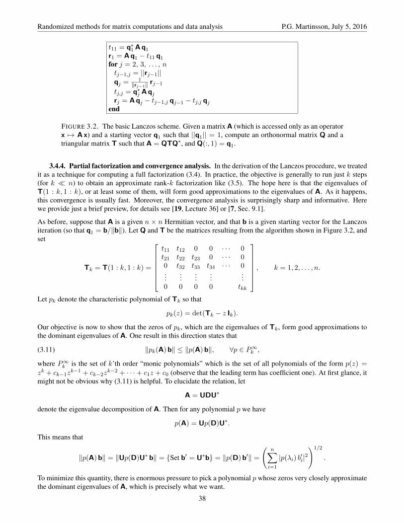
Randomized methods for matrix computations and data analysis P.G. Martinsson, July 5, 2016
t11 = q∗1 A q1
r1 = A q1 − t11 q1
for j = 2, 3, . . . , ntj−1,j = ||rj−1||qj = 1
‖rj−1‖ rj−1tj,j = q∗j A qjrj = A qj − tj−1,j qj−1 − tj,j qj
end
FIGURE 3.2. The basic Lanczos scheme. Given a matrix A (which is accessed only as an operatorx 7→ A x) and a starting vector q1 such that ||q1|| = 1, compute an orthonormal matrix Q and atriangular matrix T such that A = QTQ∗, and Q(:, 1) = q1.
3.4.4. Partial factorization and convergence analysis. In the derivation of the Lanczos procedure, we treatedit as a technique for computing a full factorization (3.4). In practice, the objective is generally to run just k steps(for k n) to obtain an approximate rank-k factorization like (3.5). The hope here is that the eigenvalues ofT(1 : k, 1 : k), or at least some of them, will form good approximations to the eigenvalues of A. As it happens,this convergence is usually fast. Moreover, the convergence analysis is surprisingly sharp and informative. Herewe provide just a brief preview, for details see [19, Lecture 36] or [7, Sec. 9.1].
As before, suppose that A is a given n × n Hermitian vector, and that b is a given starting vector for the Lanczositeration (so that q1 = b/‖b‖). Let Q and T be the matrices resulting from the algorithm shown in Figure 3.2, andset
Tk = T(1 : k, 1 : k) =
t11 t12 0 0 · · · 0t21 t22 t23 0 · · · 00 t32 t33 t34 · · · 0...
......
......
0 0 0 0 tkk
, k = 1, 2, . . . , n.
Let pk denote the characteristic polynomial of Tk so that
pk(z) = det(Tk − z Ik).
Our objective is now to show that the zeros of pk, which are the eigenvalues of Tk, form good approximations tothe dominant eigenvalues of A. One result in this direction states that
(3.11) ‖pk(A) b‖ ≤ ‖p(A) b‖, ∀p ∈ P∞k ,
where P∞k is the set of k’th order “monic polynomials” which is the set of all polynomials of the form p(z) =
zk + ck−1zk−1 + ck−2z
k−2 + · · ·+ c1z + c0 (observe that the leading term has coefficient one). At first glance, itmight not be obvious why (3.11) is helpful. To elucidate the relation, let
A = UDU∗
denote the eigenvalue decomposition of A. Then for any polynomial p we have
p(A) = Up(D)U∗.
This means that
‖p(A) b‖ = ‖Up(D)U∗ b‖ = Set b′ = U∗b = ‖p(D) b′‖ =
(n∑i=1
|p(λi) b′i|2)1/2
.
To minimize this quantity, there is enormous pressure to pick a polynomial p whose zeros very closely approximatethe dominant eigenvalues of A, which is precisely what we want.
38

Randomized methods for matrix computations and data analysis P.G. Martinsson, July 5, 2016
T11 = Q∗1 A Q1
R1 = A Q1 − T11 Q1
for j = 2, 3, . . . , r[Qj , Tj,j−1] = qr(Rj−1)Tj,j = Q∗j A Qj
Rj = A Qj − Tj−1,j Qj−1 − Tj,j Qj
end
FIGURE 3.3. The blocked Lanczos scheme. Given an n × n Hermitian matrix A and an n × bstarting matrix Q1 such that Q∗1 Q1 = Ib, the scheme computes an orthonormal matrix Q and ablock triangular matrix T such that A = QTQ∗, and Q(:, 1 : b) = Q1.
3.4.5. Block Lanczos. The scheme described in Figure 3.2 admits a simple block formulation. The set-up isentirely analogous. We seek a factorization of the form (3.4), with
Q = [Q1 Q2 · · · Qr], T =
T11 T∗21 0 0 · · ·T21 T22 T∗32 0 · · ·
0 T23 T33 T∗43 · · ·
0 0...
...
.Each block Tij is of size b× b, each block Qj is of size n× b, and we assume that there are r blocks so that n = rb(if n is not an even multiple of b the scheme can trivially be modified to allow the last block to be treated to havefewer columns). Suppose that Q1 is a given n× b orthonormal matrix. Then
Q1 T11 + Q2 T21 = A Q1.
Left multiply by Q∗1 and used that Q∗i Qj = δij I to obtain
T11 = Q∗1 A Q1.
ThenQ2 T21 = A Q1 −Q1 T11.
Now preform a QR-factorization of the right-hand side to obtain the matrices Q2 and T21. Proceed analogously.The result is given in Figure 3.3.
3.5. The Arnoldi process
Let A be an n × n matrix, not necessarily Hermitian. In this case, it is too much to ask for a factorization (3.4)where the middle factor is tridiagonal. Instead, we relax the requirements and seek a factorization
A = QHQ∗,
where H is in “Hessenberg” form
H =
h11 h12 h13 h14 · · ·h21 h22 h23 h24 · · ·
0 h32 h33 h34 · · ·0 0 h43 h44 · · ·...
......
...
.The derivation follows the Lanczos derivation completely. Rewrite the factorization as
(3.12) AQ = QH.
The first column of (3.12) evaluates to
(3.13) A q1 = q1 h11 + q2 h21.
Multiplying from the left by q∗1 we findh11 = q∗1 A q1.
39
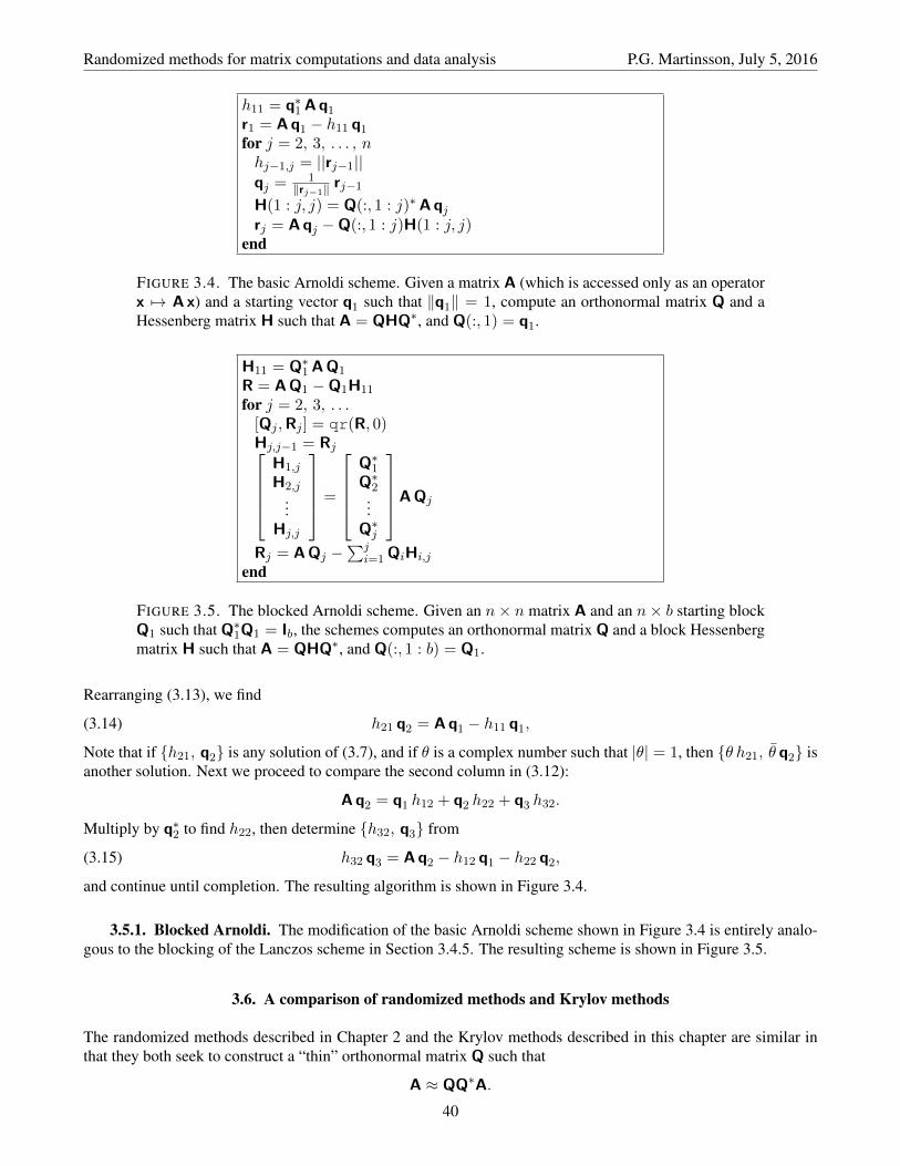
Randomized methods for matrix computations and data analysis P.G. Martinsson, July 5, 2016
h11 = q∗1 A q1
r1 = A q1 − h11 q1
for j = 2, 3, . . . , nhj−1,j = ||rj−1||qj = 1
‖rj−1‖ rj−1H(1 : j, j) = Q(:, 1 : j)∗A qjrj = A qj −Q(:, 1 : j)H(1 : j, j)
end
FIGURE 3.4. The basic Arnoldi scheme. Given a matrix A (which is accessed only as an operatorx 7→ A x) and a starting vector q1 such that ‖q1‖ = 1, compute an orthonormal matrix Q and aHessenberg matrix H such that A = QHQ∗, and Q(:, 1) = q1.
H11 = Q∗1 A Q1
R = A Q1 −Q1H11
for j = 2, 3, . . .[Qj ,Rj ] = qr(R, 0)Hj,j−1 = Rj
H1,j
H2,j...
Hj,j
=
Q∗1Q∗2...
Q∗j
A Qj
Rj = A Qj −∑j
i=1 QiHi,j
end
FIGURE 3.5. The blocked Arnoldi scheme. Given an n× n matrix A and an n× b starting blockQ1 such that Q∗1Q1 = Ib, the schemes computes an orthonormal matrix Q and a block Hessenbergmatrix H such that A = QHQ∗, and Q(:, 1 : b) = Q1.
Rearranging (3.13), we find
(3.14) h21 q2 = A q1 − h11 q1,
Note that if h21, q2 is any solution of (3.7), and if θ is a complex number such that |θ| = 1, then θ h21, θ q2 isanother solution. Next we proceed to compare the second column in (3.12):
A q2 = q1 h12 + q2 h22 + q3 h32.
Multiply by q∗2 to find h22, then determine h32, q3 from
(3.15) h32 q3 = A q2 − h12 q1 − h22 q2,
and continue until completion. The resulting algorithm is shown in Figure 3.4.
3.5.1. Blocked Arnoldi. The modification of the basic Arnoldi scheme shown in Figure 3.4 is entirely analo-gous to the blocking of the Lanczos scheme in Section 3.4.5. The resulting scheme is shown in Figure 3.5.
3.6. A comparison of randomized methods and Krylov methods
The randomized methods described in Chapter 2 and the Krylov methods described in this chapter are similar inthat they both seek to construct a “thin” orthonormal matrix Q such that
A ≈ QQ∗A.
40

Randomized methods for matrix computations and data analysis P.G. Martinsson, July 5, 2016
The two classes of techniques are similar in that the both interact with A only via its action on given sets of vectorsor thin matrices. (For non-Hermitian matrices, the randomized techniques also need application of A∗, whileKrylov methods generally do not.)
Let us first compare a basic single-vector Krylov method (e.g. Figure 3.4) with the basic randomized method(e.g. Figure 2.1). To keep the comparison simple, suppose that we take ` steps of the Krylov method, and use aGaussian random matrix with ` columns in the randomized scheme. Then, to simplify greatly, the methods compareas follows:
Basic RSVD scheme (Figure 2.1) Basic Arnoldi scheme (Figure 3.4)Interaction with A: ` matrix-vector multiplications that can all
be executed independently of each other.In particular, they can be executed in par-allel as a matrix-matrix multiplication.
` matrix-vector multiplications that haveto be executed consecutively, one at a time.
Speed: For a fixed `, faster. For a fixed `, slower.Accuracy: For a fixed ` less accurate, in particular if
the singular values decay slowly.For a fixed `, more accurate.
Other: Also requires application of A∗ to ` vec-tors.
Can sometimes get high accuracy not onlyon leading singular values, but also on thesmallest ones.
The randomized power method described in Section 2.7 and the blocked Krylov methods described in Sections3.4.5 and 3.5.1 represent two ways to bridge the gap between the extreme versions of the algorithms to obtainhybrid methods that have some of the best qualities of both schemes. These methods are conceptually very close(in particular the randomized method with an “extended sampling matrix” described in Section 2.7.3). The keypoint here is that by using a Gaussian random matrix as the starting point, one can often get away with taking avery small number of steps in the “power iteration” and thereby increasing computational speed (primarily througha reducing the amount of communication required).
3.7. Exercises
EXERCISE 1. Suppose that A is a real n × n symmetric matrix with eigenpairs λj , vjnj=1, ordered so that|λ1| ≥ |λ2| ≥ · · · ≥ |λn|. Define a sequence of vectors via x0 = randn(n, 1), and then xp = Axp−1, so thatxp = Apx0.
(a) Set β = |λ2|/|λ1| and yp = (1/‖xp‖) xp. Assume that λ1 = 1 and that β < 1. Prove that as p→∞, thevectors yp converge either to v1 or to −v1.
(b) What is the speed of convergence of yp?(c) Assume again that β = |λ2|/|λ1| < 1, but now drop the assumption that λ1 = 1. Prove that your answers
in (a) and (b) are still correct, with the exception that if λ1 is negative, then it is the vector (−1)pyp thatconverges instead.
In solving this problem, you are allowed to use that when x0 is drawn from a Gaussian distribution (which is whatthe Matlab command randn does) it has a series expansion x0 =
∑nj=1 cj vj where cj 6= 0 with probability 1. (In
fact, one can prove that each cj is a random variable drawn from a normalized Gaussian distribution.)
41


CHAPTER 4
Interpretation of data: The CUR and Interpolative Decompositions
4.1. The interpolative decomposition
4.1.1. Basic idea. Any matrix A of size m×n and rank k, where k < min(m,n), admits a so call “interpola-tive decomposition (ID)” which takes the form
(4.1)A = C Z,
m× n m× k k × n
where the matrix C is given by a subset of the columns of A and where Z is well-conditioned in a sense that wewill make precise shortly. The ID has several advantages, as compared to, e.g., the QR or SVD factorizations:
• If A is sparse or non-negative, then C shares these properties.• The ID require less memory to store than either the QR or the SVD.• Finding the indices associated with the spanning columns is often helpful in data interpretation.• In the context of numerical algorithms for discretizing PDEs and integral equations, the ID often preserves
“the physics” of a problem in a way that the QR or SVD do not.
One shortcoming of the ID is that when A is not of precisely rank k, then the approximation error by the bestpossible rank-k ID can be substantially larger than the theoretically minimal error. (In fact, the ID and the columnpivoted QR factorizations are closely related, and they attain exactly the same minimal error.)
4.1.2. Notation. While the ID is in many ways a very “natural” factorization, the notation required to fullydescribe it is slightly cumbersome. Consider again the factorization (4.1). We let Js denote an index vector oflength k that identifies the k columns that form C so that
C = A(:, Js).
The columns listed in Js are called the “skeleton” columns. We put the remaining indices in a vector of “residual”indices Jr so that we obtain a disjoint partitioning of the index set
[1, 2, 3, . . . , n] = Js ∪ Jr.
Next observe that the relation (4.1) implies that the matrix Z must contain as a submatrix the k × k identity matrixIk. Specifically, restricting (4.1) to the k columns identified in Js, we see that it must necessarily be the case that
Z(:, Js) = Ik.
The remaining n− k columns of Z consist of a k × (n− k) matrix
T = Z(:, Jr).
We refer to the entries of T as expansion coefficients since each column of T contains the expansion coefficientsused to build the corresponding column of A using the k skeleton columns as a basis. Finally, let P denote then× n permutation matrix defined by P = In(:, [Js, Jr]), so that
AP = A(:, [Js, Jr]) =[C,A(:, Jr)
].
ThenZ =
[Ik T
]P∗.

Randomized methods for matrix computations and data analysis P.G. Martinsson, July 5, 2016
4.1.3. Three flavors of ID: The row, column, and double-sided ID. Sections 4.1.1 and 4.1.2 describe afactorization where we use a subset of the columns of A to space its column space. Naturally, this factorization hasa sibling which uses the rows of A to span its row space. In other words A also admits the factorization
(4.2)A = X R,
m× n m× k k × nwhere R is a matrix consisting of k rows of A, and where X is a matrix that contains the k × k identity matrix. Welet Is denote the index vector of length k that marks the “skeleton” rows so that R = A(Is, :).
Finally, there exists a so called double-sided ID which takes the form
(4.3)A = X As Z,
m× n m× k k × k k × nwhere X and Z are the same matrices as those that appear in (4.1) and (4.2), and where As is the k × k submatrixof A given by
As = A(Is, Js).
In this chapter, we will for the most part discuss techniques for computing the column ID. With very minor modi-fications, these techniques can be used to compute the row ID and the double-sided ID too.
4.1.4. Storage requirements of the ID. Suppose that A is dense. Then we find that the amount of storagerequired to store the various factors are:
• Row-ID: Storing R and X require kn and k(m− k) floats, respectively.• Column-ID: Storing C and Z require km and k(n− k) floats, respectively.• Double-ID: Storing As, X, and Z require k2, k(m− k), and k(n− k) floats, respectively.
In every case, the storage requirements add up to k(m+ n− k). This is slightly better than the cost of storing theQR or SVD factorizations (which are k(m+ n− k/2) and k(m+ n), respectively).
For sparse matrices, the storage advantage of the ID becomes more dramatic. In this case, C and R will be sparsetoo, which can greatly cut down on the cost. For the double-sided ID, we can play some games to further reducestorage requirements. Suppose that A has exact rank k, and has a column ID
(4.4) A = CZ,
where C = A(:, Js). Suppose further that we find a good set Is of spanning rows of C, as we do in constructing thedoublesided ID. Then restrict (4.4) to the rows in Is to obtain
(4.5) A(Is, :) = C(Is, :)Z.
Now observe that C(Is, :) = A(Is, Js) to find that Z satisfies the relation
(4.6) A =(A(Is, Js)
)−1A(Is, :).
In order to use the factorization (4.4), we see that there is no need to store Z explicitly: We only need A(Is, :) and(A(Is, Js)
)−1, which are both cheap to store (since A(Is, :) is sparse, and(A(Is, Js)
)−1 is tiny).
REMARK 4.1. In some environments, it is not necessary to store C and R explicitly. If the matrix entries are cheapto generate on the fly, then it is enough to just store the index vectors Is and Js.
4.2. Existence of the ID
That any matrix of precise rank k admits factorization like (4.1), (4.2), and (4.3), is a direct consequence of thedefinition of the concept of rank.1 A slightly deeper result is that there must always exist a well-conditioned ID. Tobe precise, we will prove that there exist IDs for which every entry of the “basis matrices” X and Z is bounded inmodulus by one.
1Suppose A has rank k, so that its column space has dimension k. This means that the set of columns of A must contain a set of atleast k independent vectors (otherwise the rank would be less than k). Once a set of k linearly independent columns has been fixed, we seethat any of the remaining columns can be expressed as a linear combination of the chosen k (otherwise the rank would be higher than k).
44

Randomized methods for matrix computations and data analysis P.G. Martinsson, July 5, 2016
THEOREM 9. Let A be an m×n matrix of precisely rank k, where k < min(m,n). Then A admits a factorization
(4.7)A = C Z,
m× n m× k k × nwhere C = A(:, Js) for some index vector Js of length k contained in [1, 2, . . . , n], and where
maxi,j|Z(i, j)| ≤ 1.
PROOF. Let us first consider a special case where m = k so that A is of size k × n. Then define the indexvector Js as the set of k indices that maximize the determinant of A(:, Js). In other words:
(4.8) Js = argmax|det(A(:, J))| : J is a subset of size k of [1, 2, . . . , n].(The max may or may not unique, this does not matter.) Let Jr denote an index vector containing the “remaining”indices so that Js ∪ Jr = [1, 2, . . . , n] in a disjoint union. Let P denote the permutation matrix for which
(4.9) AP = [A(:, Js) A(:, Jr)].
Observe that A(:, Js) must be non-singular, so we can rewrite (4.9) as
(4.10) AP = A(:, Js) [Ik A(:, Js)−1A(:, Jr)].
Setting
(4.11) T := A(:, Js)−1A(:, Jr),
we find that we can write (4.10) as
(4.12) A = A(:, Js)︸ ︷︷ ︸=:C
[Ik T]P∗︸ ︷︷ ︸=:Z
.
We will next prove that every element of T has modulus at most one. Let jini=1 denote the chosen permutationof [1, 2, . . . , n] such that
[Js Jr] = [j1 j2 j3 · · · jn].
We now find that the definition of T in (4.11) implies that[cj1 cj2 · · · cjk
]︸ ︷︷ ︸=A(:,Js)
T =[cjk+1
cjk+2· · · cjn
]︸ ︷︷ ︸=A(:,Jr)
.
Cramer’s rule provides us with explicit solution formulas for each element of T. For instance,
T(1, 1) =det[cjk+1
cj2 cj3 cj4 · · · cjk]
det[cj1 cj2 cj3 cj4 · · · cjk
] , T(1, 2) =det[cjk+2
cj2 cj3 cj4 · · · cjk]
det[cj1 cj2 cj3 cj4 · · · cjk
] ,T(2, 1) =
det[cj1 cjk+1
cj3 cj4 · · · cjk]
det[cj1 cj2 cj3 cj4 · · · cjk
] , T(2, 2) =det[cj2 cjk+2
cj3 cj4 · · · cjk]
det[cj1 cj2 cj3 cj4 · · · cjk
] ,et cetera. Observe that in each formula, the denominator consists of the determinant formed by the k columns ofA that maximize the modulus of the determinant. The numerator is obtained by swapping out one of the columnsfrom the maximizing set by a different column. It follows directly from the definition of Js in (4.8) that each suchratio must be bounded by one in modulus.
All that remains is to relax our temporary assumption that the matrix A must have precisely k rows. In the generalcase, observe that when A has exact rank k, it admits a factorization
(4.13)A = E F,
m× n m× k k × nfor some matrices E and F (their properties do not matter beyond the fact that they both have precise rank k). Wehave shown that F admits an ID factorization with the required properties, that is,
(4.14)F = F(:, Js) Z,
k × n k × k k × n45

Randomized methods for matrix computations and data analysis P.G. Martinsson, July 5, 2016
where every entry of Z is bounded by one in modulus. Combining (4.13) and (4.14) we get
(4.15) A = EF(:, Js)Z.
Since Z(:, Js) = Ik, we can restrict (4.15) to the columns in Js to see that
(4.16) A(:, Js) = EF(:, Js),
Combining (4.15) and (4.16) we finally get
(4.17) A = A(:, Js)Z,
which is the factorization we sought.
4.3. Deterministic techniques for computing the ID
4.3.1. Computing the ID from the column pivoted QR. The ID and the column pivoted QR factorization(CPQR) are closely related. To demonstrate this, let A be an m× n matrix. At first, let us assume that A has exactrank k, and that we have computed its CPQR so that
(4.18)A(:, J) = Q1 R.m× n m× k k × n
(Our choice to endow the “Q” factor with a subscript is to keep notation consistent with the general case where Adoes not have exact rank k.) Now let us partition
J =[Js Jr
],(4.19)
R =[R11 R12
],(4.20)
in such a way that Js holds the first k indices in J , and R11 is the leading k × k submatrix of R. Observe that Jspoints to the k columns on A that were chosen as “pivots.” Set
(4.21) C = A(:, Js).
Then (4.18) can be written
(4.22)[C A(:, Jr)
]=[Q1R11 Q1R12
].
Looking at the first k columns of (4.22) we see that it must be the case that
C = Q1R11.
Next, observe that R11 is necessarily invertible (since A has rank k, and the pivoting procedure ensures that thecolumns in C are linearly independent). This means that (4.22) can be rewritten as
(4.23) A = C[Ik T
]P∗︸ ︷︷ ︸
=:Z
,
where P is the permutation matrix associated with J (as usual), and where
(4.24) T := R−111 R12.
Equation (4.23) tells us that the CPQR factorization is in fact an ID in (very slight) disguise.
Next let us consider the case where A does not have exact rank k. Suppose that we have computed the full CPQR,which then takes then form
(4.25) A(:, J) =[Q1 Q2
] [ R11 R12
0 R22
],
where Q1 holds the first k columns of Q and R11 is k × k. Let us again partition the index vector as dictated by(4.19), define C via (4.21), and T via (4.24). Then we obtain the approximate rank-k factorization
A ≈ Q1
[R11 R12
]P∗ = Q1R11
[Ik R−111 R12
]P∗ = C
[Ik T
]P∗ = C Z.
We also have an exact expression for the approximation error from (4.25):
A− CZ = QRP∗ −Q1
[R11 R12
]P∗ =
[Q1 Q2
] [ R11 R12
0 R22
]P∗ −Q1
[R11 R12
]P∗ =
[0 Q2R22
]P∗.
46

Randomized methods for matrix computations and data analysis P.G. Martinsson, July 5, 2016
In other words, the approximation error in the ID is ‖[0 Q2R22
]P∗‖ = ‖R22‖, which is exactly the same as the
approximation error in the truncated CPQR from which we obtained it.
REMARK 4.2. In practice, one typically only take k steps of the CPQR algorithm. At that point, we have a partialfactorization
AP ≈ Q1
[R11 R12] +
[0 B]
where B contains the parts of the n− k non-pivot columns that remain after projecting away from the span of Q1.Clearly BP = Q2R22 for some permutation matrix P, but one does not need to carry out these steps in order todetermine the approximation error since ‖B‖ = ‖R22‖.
4.3.2. Optimality of the QR procedure.
4.3.3. Computing the row ID and the double sided ID. First observe that the row ID is obtained by applyingthe procedure described in Section 4.3.1 to the rows of A. In other words, the first step is to compute a partial CPQRof A∗.
For the double sided ID, we start by computing a column ID,
(4.26) A = A(:, Js) Z + E,
for some “error matrix” E. Then simply compute a row ID of the matrix C = A(:, Js) containing the k chosencolumns,
(4.27) A(:, Js) = X A(Is, Js).
Observe that this second factorization is exact since the matrix A(:, Js) has k columns, and therefore necessarilyhas rank k (provided that A has rank at least k). Combining (4.26) and (4.27), we obtain
(4.28) A = A(:, Js) Z + E = XA(Is, Js) Z + E,
which is the double-sided ID we sought. Observe that the error term E is identical in (4.26) and (4.28); in otherwords, the error in the double-sided ID is identical to the error in the one-sided ID with which we start (which inturn is identical to the error in the original CPQR).
The three algorithms for computing the three flavors of the ID via the CPQR are summarized in Figure 4.1.
REMARK 4.3. The double-sided ID could also be computed by independently computing the row and column IDsof the original matrix A, as follows:
(4.29) [Js, Z] = ID col(A, k) and [Is, X] = ID row(A, k).
Then we automatically find thatA ≈ X A(Is, Js) Z.
While there are circumstances where this procedure may be beneficial, it is in general more expensive to execute.Moreover, the method in Figure 4.1 is guaranteed to produce a factorization whose approximation error is exactlythe same as the error incurred by the first column pivoted ID. Computing the double sided ID via (4.25) involvestwo independent approximations that each incurs its own error; these two errors combine to a form an overall errorthat can easily exceed that of the method in Figure 4.1.
4.4. Computing interpolative decompositions via randomized sampling
The randomized range finder described in Section 2.3 is particularly effective when used in conjunction with theinterpolative decomposition. To illustrate the process, consider for a moment the task of factorizing an m × nmatrix A of exact rank k (we will discuss the case of approximate rank shortly). Using the randomized samplingtechnique, we would then draw an n × k random matrix G, form a sample matrix Y = AG, orthonormalize itscolumns to form the matrix Q = orth(Y), and finally form the rank-k factorization
A ≈ Q(Q∗A
).
47

Randomized methods for matrix computations and data analysis P.G. Martinsson, July 5, 2016
Compute a column ID so that A ≈ A(:, Js) Z.function [Js, Z] = ID col(A, k)
[Q,R, J ] = qr(A, 0);T = (R(1 : k, 1 : k))−1R(1 : k, (k + 1) : n);Z = zeros(k, n)Z(:, J) = [Ik T];Js = J(1 : k);
Compute a row ID so that A ≈ X A(Is, :).function [Is, X] = ID row(A, k)
[Q,R J ] = qr(A∗, 0);T = (R(1 : k, 1 : k))−1R(1 : k, (k + 1) : n);X = zeros(m, k)X(J, :) = [Ik T]∗;Is = J(1 : k);
Compute a double-sided ID so that A ≈ X A(Is, Js) Z.function [Is, Js,X,Z] = ID double(A, k)
[Js, Z] = ID col(A, k);[Is, X] = ID row(A(:, Js), k);
FIGURE 4.1. Deterministic algorithms for computing the column, row, and double-sided ID viathe column pivoted QR factorization. The input is in every case an m × n matrix A and a targetrank k. Since the algorithms are based on the CPQR, it is elementary to modify them to thesituation where a tolerance rather than a rank is given. (Recall that the errors resulting from theseID algorithms are identical to the error in the first CPQR factorization executed.)
This process requires the evaluation of the matrix-matrix product Q∗A. It turns out that by using the ID instead,we can skip this step. Instead of applying Gram-Schmidt to the columns of Y, we apply Gram-Schmidt to the rowsof Y to find a good spanning set of rows. To be precise, we execute the command rows,
[X, Is] = ID row(Y, k).
Then
(4.30) Y = XY(Is, : ).
Now, automatically (!), the couple X, Is also forms an ID for A,
(4.31) A = XA(Is, : ).
(See Remark 4.4 for details.) The beauty here is that once we have the sample matrix Y, we do not need to revisitall of A to construct a rank-k factorization — all we need to do is to extract the k rows of A indicated by the indexvector Is.
By combining the idea of using an SRFT for “Stage A” (at complexity O(mn log(k))) with an ID for “Stage B” (atcomplexity O((m+ n)k2)), we get the accelerated algorithm for constructing an ID described in Figure 4.3. Witha slight modification to Stage B, we get the O(mn log(k)) algorithm for computing an SVD described in Figure4.4. More details (including an error analysis for the case when A has only approximate rank k) can be found in[11, Sec. 5.2].
REMARK 4.4. It is perhaps not immediately clear why the ID X, Is computed for Y should automatically alsobe an ID for A. To see why this should be, first observe that since the columns of Y form a basis for the columnsof A, there must exist a k × n matrix F such that
(4.32) A = YF.
Now insert the relation (4.30) into (4.32):
(4.33) A = XY(Is, : )F.
48

Randomized methods for matrix computations and data analysis P.G. Martinsson, July 5, 2016
ALGORITHM: RANDOMIZED ID
Inputs: An m× n matrix A, a target rank k, an over-sampling parameter p (say p = 10), and a small integerq denoting the number of power iterations taken.
Outputs: An m× k interpolation matrix X and an index vector Is ∈ Nk such that A ≈ XA(Is, : ).
(1) G = randn(n, k + p);(2) Y = AG;(3) for j = 1 : q
(4) Z = A∗Y;
(5) Y = AZ;
(6) end for(7) Form an ID of the n× (k + p) sample matrix: [X, Is] = ID row(Y, k).
FIGURE 4.2. An O(mnk) algorithm for computing an interpolative decomposition of A via ran-domized sampling. For q = 0, the scheme is fast (but not quite as fast as the scheme in Figure 4.3)and accurate for matrices whose singular values decay rapidly. For matrices whose singular valuesdecay slowly, one should pick a larger q (say q = 1 or 2) to improve accuracy at the cost of longerexecution time. If accuracy better than ε1/(2q+1)
mach is desired, then the scheme should be modified toincorporate orthonormalization as described in Remark 2.5.
ALGORITHM: FAST RANDOMIZED ID
Inputs: An m× n matrix A, a target rank k, and an over-sampling parameter p (say p = k).
Outputs: An m× k interpolation matrix X and an index vector Is ∈ Nk such that A ≈ XA(Is, : ).
Stage A:(1) Form an n× (k + p) SRFT Ω.(2) Form the sample matrix Y = A Ω.
Stage B:(3) Form an ID of the n× (k + p) sample matrix: [X, Is] = ID row(Y, k).
FIGURE 4.3. An O(mn log(k)) algorithm for computing an interpolative decomposition of A.
Restrict (4.33) to the rows in Is, and exploit that X(Is, :) = Ik to find
(4.34) A(Is, :) = X(Is, :)Y(Is, : )F = Y(Is, : )F.
Finally, insert (4.34) in (4.33) to attain (4.31).
4.5. The CUR Decomposition
4.5.1. Basic definitions. A rank k CUR factorization of a matrix A ∈ Cm×n is given by
A ≈ C U R,m× n m× k k × k k × n
where C = A(:, Js) consists of k columns of A, and R = A(Is, :) consists of k rows of A. The decomposition istypically obtained in three steps [16]: (1) Some scheme is used to assign a weight or the so called leverage score(of importance) to each column and row in the matrix. This is typically done either using the `2 norms of thecolumns and rows or by using the leading singular vectors of A [5]. (2) The matrices C and R are constructed via
49

Randomized methods for matrix computations and data analysis P.G. Martinsson, July 5, 2016
ALGORITHM: FAST RANDOMIZED SVD
Inputs: An m× n matrix A, a target rank k, and an over-sampling parameter p (say p = k).
Outputs: Matrices U, Σ, and V in an approximate rank-(k + p) SVD of A. (I.e. U and V are orthonormaland Σ is diagonal.)
Stage A:(1) Form an n× (k + p) SRFT Ω.(2) Form the sample matrix Y = B Ω.
Stage B:(3) Form an ID of the sample matrix Y: [X, Is] = ID row(Y, k).(4) Compute the QR decomposition of the interpolation matrix [Q,R] = qr(X).(5) Extract k + p rows of A: Arows = A(Is, :).(6) Multiply R and Arows to form the (k + p)× n matrix F = RArows.(7) Decompose the matrix F in a singular value decomposition [U, Σ, V] = svd(F).(8) Form U = QU.
FIGURE 4.4. AnO(mn log(k)) algorithm for computing a partial SVD. If an SVD of exactly rankk is desired, then truncate the factors computed in Step (7).
a randomized sampling procedure, using the leverage scores to assign a sampling probability to each column androw. (3) The U matrix is computed via:
(4.35) U ≈ C†AR†,
with C† and R† being the pseudoinverses of C and R.
Many techniques for computing CUR factorizations have been proposed. In particular, we mention the recent workof Sorensen and Embree [17] on the DEIM-CUR method. A number of standard CUR algorithms is implementedin the software package rCUR [2]. The methods in the rCUR package utilize eigenvectors to assign weights tocolumns and rows of A. Computing the eigenvectors exactly amounts to doing the SVD which is very expensive.However, instead of the full SVD, when a CUR of rank k is required, we can utilize instead the randomized SVDalgorithm [11] to compute an approximate SVD of rank k at substantially lower cost.
4.5.2. Conditioning of CUR. For matrices whose singular value experience substantial decay, the accuracyof the CUR factorization can deteriorate due to effects of ill-conditioning. To simplify slightly, one would normallyexpect the leading k singular values of C and R to be roughly similar in size to the leading k singular values ofA. Since low-rank factorizations are most useful when applied to matrices whose singular values decay reasonablyrapidly, we would typically expect C and R to be highly ill-conditioned, with condition numbers roughly on theorder of σ1(A)/σk(A). Hence, in the typical case, evaluation of the formula (4.35) can be expected to result insubstantial loss of accuracy due to accumulation of round-off errors. Observe that the ID does not suffer from thisproblem; in (4.3), the matrix Askel tends to be ill-conditioned, but it does not need to be inverted. (The matrices Xand Z are well-conditioned.)
Example: Consider an m× n matrix A of rank 2, whose doublesided ID is given by
(4.36) A = XAsY, where X =
[IS
], Y =
[I T
], As =
[1 00 β
],
for some small number β. Then the CUR factorization of A takes the form
(4.37) A = A(:, [1, 2])
[1 00 1/β
]A([1, 2], :).
Observe that while the factorization (4.36) is perfectly well-conditioned, the factorization (4.37) is numericallyproblematic whenever β is small.
50

Randomized methods for matrix computations and data analysis P.G. Martinsson, July 5, 2016
4.5.3. Storage requirements of CUR and ID. For a dense matrix, all matrix decompositions that we havediscussed require roughly k(m+ n) floats. When k is close to m and n in size, then terms of order k2 matter too,and we find that the precise requirements are (cf. Section 4.1.4):
Number of floats required to store a dense m× n matrix of rank k:CUR SVD QR ID (all three flavors)
Storage requirement: k(m+ n+ k) k(m+ n) k(m+ n− k/2) k(m+ n− k)
In other words, the CUR is the most expensive, and the ID is the least expensive.
When A is sparse, then the ID and the CUR decomposition gain a large advantage since the factors C and R inheritsparsity from the original matrix. At first glance, the ID might seem more expensive in this requirement since itappears to require the storage of the dense matrices of expansion coefficients X, Z, or both. But, as we showed inSection 4.1.4, this problem can easily be fixed, so that the CUR and the ID have the same storage requirements:
Storage requirements of CUR and ID: One dense k × k matrix, and k rows and k columns of A.
4.6. Deterministic techniques for computing the CUR
In this section, we describe a deterministic technique we label the CUR-ID for computing the CUR factorizationfrom the double-sided ID. We start with a heuristic derivation in Section 4.6.1, and then proceed to prove that theerror incurred is modest in Section 4.6.2.
4.6.1. Converting a double-sided ID to a CUR decomposition. The CUR-ID algorithm is based on thedouble-sided ID and as a starting point, we assume the factorization (4.3) has been computed using the proceduresdescribed in Section 4.3.3. In other words, we assume that the index vectors Is and Js, and the basis matrices Xand Z, are all available. We then define
(4.38) C = A(:, Js) and R = A(Is, :).
Consequently, C and R are respectively subsets of columns and of rows of A, with Js and Is determined by thecolumn pivoted QR factorizations. Next we construct a k × k matrix U such that A ≈ CUR. We know that
(4.39) A ≈ C Z,
and we seek a factor U such that
(4.40) A ≈ C U R.
By inspecting (4.39) and (4.40), we find that we achieve our objective if we determine a matrix U such that
(4.41)U R = Z.
k × k k × n k × nUnfortunately, (4.41) is an over-determined system, but at least intuitively, it seems plausible that it should have afairly accurate solution, given that the rows of R and the rows of Z should, by construction, span roughly the samespace (namely, the space spanned by the k leading right singular vectors of A). Solving (4.41) in the least-squaresense, we arrive at our definition of U:
(4.42) U := ZR†.
The resulting algorithm is summarized in Figure 4.5.
REMARK 4.5. Observe that for purposes of data interpretation, the double-sided ID is just as useful as the CUR,and does not suffer from problems of ill-conditioning, cf. Section 4.5.2.
REMARK 4.6. The techniques for computing the double sided ID that we have described are based on two single-sided IDs. Observe that these can be executed in a few different ways. For instance, either of the following twomethods work well:
51

Randomized methods for matrix computations and data analysis P.G. Martinsson, July 5, 2016
ALGORITHM: CUR FROM COLUMN PIVOTED QR
Inputs: An m× n matrix A, and a target rank k.
Outputs: A k × k matrix U, and index vector Is and Js such that A ≈ A(:, Js)UA(Is, :).
(1) [Is, Js,X,Z] = ID double(A, k).(2) U = Z(A(Is, :))
†.
FIGURE 4.5. An algorithm for computing a CUR factorization via two column pivoted QR fac-torizations. Very important: When the double-sided ID is constructed, it is in this context crucialthat the second ID is performed only the subset of columns picked by the first ID, not on the fullmatrix, see Remark 4.6.
Method 1: Method 2:[Js, Z] = ID col(A, k); [Js, Z] = ID col(A, k);[Is, X] = ID row(A(:, Js), k); [Is, X] = ID row(A, k);
The first step of both methods is the same: perform CPQR on the columns of A to find the spanning columns.In the second step, Method 1 performs a row ID using only the columns chosen in the first step, while Method2 performs a row ID on all of A. For purposes of computing the double-sided ID, we generally recommend theuse of Method 1 since it is computationally more efficient, but either method works fine. When we compute theCUR decomposition, however, it is crucial that Method 1 is used. The reason is that Method 1 inherently seeks toconstruct a matrix A(Is, Js) that is as well conditioned as possible. When using Method 2, one can easily end upwith a matrix A(Is, Js) that is far worse conditioned than is necessary.
4.6.2. Error analysis of the CUR-ID algorithm. The construction of C, U, and R in Section 4.6.1 was basedon heuristics. We next demonstrate that the approximation error is comparable to the error resulting from theoriginal QR-factorization. First, let us define E and E as the errors in the column and row IDs of A, respectively,
A = C Z + E,(4.43)
A = X R + E.(4.44)
Recall that E is a quantity we can control by continuing the original QR factorization of A until ‖E‖ is smallerthan some given threshold. We will prove that ‖E‖ cannot be all that much larger than ‖E‖, which leads us to thefollowing error bound for the algorithm in Figure 4.5:
THEOREM 10. Let A be an m × n matrix. Suppose that we have computed a column ID of rank k for A witherror term E, as in (4.43). Suppose further that we next compute the row ID Is,X of C, and use this row ID toapproximate A, resulting in an approximation error E, as in (4.44). Then
(4.45) ‖E‖ ≤ (1 + ‖T‖) ‖E‖,
where T is the k×(m−k) matrix of expansion coefficients obtained while computing the row ID of C. Additionally,it holds that
(4.46) ‖A− CUR‖ ≤ (2 + ‖T‖) ‖E‖.
The error bound in Theorem 10 involves the term ‖T‖. We can provide a simplistic bound for this quantity asfollows: Recall that the matrix T contains the expansion coefficients in the interpolative decomposition of C.These can be guaranteed [8, 12] to all be bounded by 1 + ν in magnitude for any positive number ν. The costincreases as ν → 0, but for, e.g., ν = 1, the cost is very modest. Consequently, we find that for either the spectralor the Frobenius norm, we can easily guarantee ‖T‖ ≤ (1 + ν)
√k(n− k), with practical norm often far smaller.
We will prove Theorem 10 in two steps. Lemma 11 asserts that when (4.43) and (4.44) hold, then ‖A− CUR‖ ≤E + E. Then Lemma 12 provides the information we need to bound ‖E‖.
52

Randomized methods for matrix computations and data analysis P.G. Martinsson, July 5, 2016
LEMMA 11. Let A be an m × n matrix that satisfies the approximate factorizations (4.43) and (4.44). Supposefurther that R is full rank, and that the k × k matrix U is defined by (4.42). Then
(4.47) ‖A− CUR‖ ≤ ‖E‖+ ‖E‖.
PROOF. Using first (4.42) and then (4.43), we find
(4.48) A− CUR = A− CZR†R = A− (A− E)R†R =(A− AR†R
)+ ER†R.
To bound the term A− AR†R we use (4.44) and the fact that RR†R = R to achieve
(4.49) A− AR†R = A− (WR + E)R†R = A−WR− ER†R = E− ER†R = E(I− R†R).
Inserting (4.49) into (4.48) and taking the norms of the result, we get
‖A− CUR‖ = ‖E(I− R†R) + ER†R‖ ≤ ‖E(I− R†R)‖+ ‖ER†R‖ ≤ ‖E‖+ ‖E‖,where in the last step we used that RR† and I− RR† are both orthonormal projections.
LEMMA 12. Let A be an m × n matrix that admits the factorization (4.43), with error term E. Suppose furtherthat I = [Is, Ir] and T form the output of the row ID of the matrix C, so that
(4.50) C = XC(Is, :), where X = P
[I
T∗
],
and where P is the permutation matrix for which PA(I, :) = A. Now define the matrix R via
(4.51) R = A(Is, :).
Observe that R consists of the k rows of A selected in the skeletonization of C. Finally, set
(4.52) F =[−T∗ I
]P∗.
Then the product XR approximates A, with a residual error
(4.53) E = A− XR = P
[0
FE
].
PROOF. From the definitions of X in (4.50) and R in (4.51) we find
(4.54) A− XR = PA(I, :)− XR = P
[A(Is, :)A(Ir, :)
]− P
[I
T∗
]A(Is, :)
= P
[0
A(Ir, :)− T∗A(Is, :)
]= P
[0
FA
].
To bound the term FA in (4.54), we invoke (4.43) to obtain
(4.55) FA = FCV∗ + FE = Insert (4.50) = FXC(Is, :)V∗ + FE = FE,
since FX = 0 due to (4.50) and (4.52). Finally, insert (4.55) into (4.54) to obtain (4.53).
PROOF OF THEOREM 10. Equation (4.53) allows us to bound the norm of the error E in (4.44). Simply ob-serve that the definition of F in (4.52) implies that for any matrix B we have:
FB =[−T∗ I
]P∗B =
[−T∗ I
] [B(Is, :)B(Ir, :)
]= −T∗B(Is, :) + B(Ir, :),
so that:
(4.56) ‖FB‖ = ‖B(Ir, :)− T∗B(Is, :)‖ ≤ ‖B(Ir, :)‖+ ‖T‖ ‖B(Is, :)‖ ≤ (1 + ‖T‖) ‖B‖.We can now prove (4.45), by applying the bound (4.56) to (4.53), with E in place of B:
‖E‖ =
∥∥∥∥P
[0
FE
]∥∥∥∥ ≤ ∥∥∥∥[ 0FE
]∥∥∥∥ = ‖FE‖ ≤ (1 + ‖T‖) ‖E‖.
To establish (4.46), we use (4.47) and (4.45):
‖A− CUR‖ ≤ ‖E‖+ ‖E‖ ≤ (2 + ‖T‖) ‖E‖.53

Randomized methods for matrix computations and data analysis P.G. Martinsson, July 5, 2016
ALGORITHM: RANDOMIZED CUR
Inputs: An m× n matrix A, a target rank k, an over-sampling parameter p (say p = 10), and a small integerq denoting the number of power iterations taken.
Outputs: An k × k matrix U and index vectors Is and Js of length k such that A ≈ A( : , Js) U A(Is, : ).
(1) G = randn(k + p,m);(2) Y = GA;(3) for j = 1 : q
(4) Z = YA∗;
(5) Y = ZA;
(6) end for(7) Form an ID of the (k + p)× n sample matrix: [Z, Js] = ID col(Y, k).(8) Form an ID of the m× k matrix of chosen columns: [∼, Is] = ID row(A(:, Js), k).(9) Determine the linking matrix U by solving the least squares equation UA(Is, :) = Z.
FIGURE 4.6. A randomized algorithm for computing a CUR decomposition of A via randomizedsampling. For q = 0, the scheme is fast and accurate for matrices whose singular values decayrapidly. For matrices whose singular values decay slowly, one should pick a larger q (say q = 1
or 2) to improve accuracy at the cost of longer execution time. If accuracy better than ε1/(2q+1)mach
is desired, then the scheme should be modified to incorporate orthonormalization as described inRemark 2.5.
4.7. Randomized techniques for computing the CUR
In Section 4.6 we demonstrated that the CUR decomposition of a matrix can be readily computed from a double-sided ID, as long as care is taken to ensure that the matrix A(Is, Js) at the center of the double-sided ID is as wellconditioned as possible. If we combine this scheme with the randomized method for computing the double-sidedID described in Section 4.4, we then obtain a randomized algorithm for computing the CUR decomposition. Theresulting method is shown in Figure 4.6.
54
Bibliography
[1] L Susan Blackford, Antoine Petitet, Roldan Pozo, Karin Remington, R Clint Whaley, James Demmel, Jack Dongarra, Iain Duff,Sven Hammarling, Greg Henry, et al. An updated set of basic linear algebra subprograms (blas). ACM Transactions on MathematicalSoftware, 28(2):135–151, 2002.
[2] Andras Bodor, Istvan Csabai, Michael Mahoney, and Norbert Solymosi. rCUR: an R package for CUR matrix decomposition. BMCBioinformatics, 13(1), 2012.
[3] Jack J Dongarra, Jeremy Du Croz, Sven Hammarling, and Iain S Duff. A set of level 3 basic linear algebra subprograms. ACMTransactions on Mathematical Software (TOMS), 16(1):1–17, 1990.
[4] P. Drineas and M. W. Mahoney. On the Nystrom method for approximating a Gram matrix for improved kernel-based learning. J.Mach. Learn. Res., 6:2153–2175, 2005.
[5] Petros Drineas, Michael W. Mahoney, and S. Muthukrishnan. Relative-error CUR matrix decompositions. SIAM J. Matrix Anal. Appl.,30(2):844–881, 2008.
[6] A. Frieze, R. Kannan, and S. Vempala. Fast Monte Carlo algorithms for finding low-rank approximations. J. ACM, 51(6):1025–1041,2004. (electronic).
[7] Gene H. Golub and Charles F. Van Loan. Matrix computations. Johns Hopkins Studies in the Mathematical Sciences. Johns HopkinsUniversity Press, Baltimore, MD, third edition, 1996.
[8] Ming Gu and Stanley C. Eisenstat. Efficient algorithms for computing a strong rank-revealing QR factorization. SIAM J. Sci. Comput.,17(4):848–869, 1996.
[9] N. Halko. Randomized methods for computing low-rank approximations of matrices. PhD thesis, Applied Mathematics, University ofColorado at Boulder, 2012.
[10] Nathan Halko, Per-Gunnar Martinsson, Yoel Shkolnisky, and Mark Tygert. An algorithm for the principal component analysis of largedata sets. SIAM Journal on Scientific Computing, 33(5):2580–2594, 2011.
[11] Nathan Halko, Per-Gunnar Martinsson, and Joel A. Tropp. Finding structure with randomness: Probabilistic algorithms for construct-ing approximate matrix decompositions. SIAM Review, 53(2):217–288, 2011.
[12] Edo Liberty, Franco Woolfe, Per-Gunnar Martinsson, Vladimir Rokhlin, and Mark Tygert. Randomized algorithms for the low-rankapproximation of matrices. Proc. Natl. Acad. Sci. USA, 104(51):20167–20172, 2007.
[13] Per-Gunnar Martinsson, Vladimir Rokhlin, and Mark Tygert. A randomized algorithm for the approximation of matrices. TechnicalReport Yale CS research report YALEU/DCS/RR-1361, Yale University, Computer Science Department, 2006.
[14] Per-Gunnar Martinsson, Vladimir Rokhlin, and Mark Tygert. A randomized algorithm for the decomposition of matrices. Appl. Com-put. Harmon. Anal., 30(1):47–68, 2011.
[15] P.G. Martinsson and S. Voronin. A randomized blocked algorithm for efficiently computing rank-revealing factorizations of matrices.,2015. To appear in SIAM Journal on Scientific Computation, Arxiv.org report #1503.07157.
[16] Nikola Mitrovic, Muhammad Tayyab Asif, Umer Rasheed, Justin Dauwels, and Patrick Jaillet. Cur decomposition for compression andcompressed sensing of large-scale traffic data. In Intelligent Transportation Systems-(ITSC), 2013 16th International IEEE Conferenceon, pages 1475–1480. IEEE, 2013.
[17] D. C. Sorensen and M. Embree. A DEIM Induced CUR Factorization. ArXiv e-prints, July 2014.[18] G. W. Stewart. On the early history of the singular value decomposition. SIAM Rev., 35(4):551–566, 1993.[19] Lloyd N Trefethen and David Bau III. Numerical linear algebra, volume 50. Siam, 1997.[20] Franco Woolfe, Edo Liberty, Vladimir Rokhlin, and Mark Tygert. A fast randomized algorithm for the approximation of matrices.
Applied and Computational Harmonic Analysis, 25(3):335–366, 2008.