Embed Size (px)
Citation preview

RANDOMIZED COMPLETE BLOCK DESIGN (RCBD)
Description of the Design
Probably the most used and useful of the experimental designs.
Takes advantage of grouping similar experimental units into blocks or replicates.
The blocks of experimental units should be as uniform as possible.
The purpose of grouping experimental units is to have the units in a block as uniform
as possible so that the observed differences between treatments will be largely due to
“true” differences between treatments.
Randomization Procedure
Each replicate is randomized separately.
Each treatment has the same probability of being assigned to a given experimental
unit within a replicate.
Each treatment must appear at least once per replicate.
Example
Given four fertilizer rates applied to ‘Amidon’ wheat and three replicates of each
treatment.
Rep 1 Rep 2 Rep 3
A B A A=0 kg N/ha
D A B B=50 kg N/ha
C D C C=100 kg N/ha
B C D D=150 kg N/ha
Advantages of the RCBD
1. Generally more precise than the CRD.
2. No restriction on the number of treatments or replicates.
3. Some treatments may be replicated more times than others.
4. Missing plots are easily estimated.
5. Whole treatments or entire replicates may be deleted from the analysis.

6. If experimental error is heterogeneous, valid comparisons can still be made.
Disadvantages of the RCBD
1. Error df is smaller than that for the CRD (problem with a small number of
treatments).
2. If there is a large variation between experimental units within a block, a large error
term may result (this may be due to too many treatments).
3. If there are missing data, a RCBD experiment may be less efficient than a CRD
NOTE: The most important item to consider when choosing a design is the
uniformity of the experimental units.
RCBD – No Sampling
Example
Grain yield of rice at six seeding rates (Mg/ha):
Seeding rate (kg/ha)
Rep 25 50 75 100 125 150 Y.j
1 5.1 5.3 5.3 5.2 4.8 5.3 31.0
2 5.4 6.0 5.7 4.8 4.8 4.5 31.2
3 5.3 4.7 5.5 5.0 4.4 4.9 29.8
4 4.7 4.3 4.7 4.4 4.7 4.1 26.9
Yi. 20.5 20.3 21.2 19.4 18.7 18.8 118.9
2
ijY 105.35 104.67 112.92 94.44 87.53 89.16 594.07
Step 1. Calculate the correction factor (CF).
050.5894*6
9.118.. 22
tr
YCF

Step 2. Calculate the Total SS.
02.5
)1.4...3.54.51.5(
2222
2
CF
CFYSSTotal ij
Step 3. Calculate the Replicate SS (Rep SS)
965.1
6
9.268.292.310.31
pRe
2222
2
.
CF
CFt
YSS
j
Step 4. Calculate the Treatment SS (Trt SS)
2675.1
4
8.187.184.192.213.205.20
222222
2
.
CF
CFr
YSSTrt i
Step 5. Calculate the Error SS
Error SS = Total SS – Rep SS – Trt SS
= 1.7875

Step 6. Complete the ANOVA Table
SOV Df SS MS F
Rep r-1 = 3 1.9650 0.6550 Rep MS/Error MS = 5.495**
Trt t-1 = 5 1.2675 0.2535 Trt MS/Error MS = 2.127ns
Error (r-1)(t-1) = 15 1.7875 0.1192
Total tr-1 = 23 5.0200
Step 7. Look up Table F-values for Rep and Trt:
Rep Trt
F.05;3,15 = 3.29 F.05;5,15 = 2.90
F.01;3,15 = 5.42 F.01;5,15 = 4.56
Step 8. Make conclusions.
Rep: Since Fcalc.(5.495) > FTab. at the 95 and 99% levels of confidence, we reject Ho: All
replicate means are equal.
TRT: Since Fcalc.(2.127) < FTab. at the 95 and 99% levels of confidence, we fail to reject
Ho: All treatment means are equal.
Step 9. Calculate Coefficient of Variation (CV).
%97.6
100*95.4
1192.
100*
Y
sCV
Step 10. Calculate LSD’s if necessary
There is no need to calculate a LSD for replicate since you generally are not
interested in comparing differences between replicate means.
Since the F-test for treatment was non-significant, one would not calculate the F-
protected LSD. However, if the F-test for treatment was significant, the LSD would
be:

76.0
4
)1192.0(2131.2
2
205.
r
ErrorMStLSDTRT
Significance of F-tests on Replicate
This is a valid F-test but requires careful interpretation.
If the F-test for replicate is significant, this indicates that using this design instead of
a CRD has increased the precision of the experiment.
This suggests that the scope of the experiment may have been increased since the
experiment was conducted over a wider range of conditions.
One needs to be careful when replicate effects are large because this suggests
heterogeneity of error may exist.
If replicate effects are small, this suggests that either the experimenter was not
successful in reducing error variance of the individual experimental units or that the
experimental units were homogenous to start.
To know which situation is true in your case, you need to have the experience of
knowing the “typical” size of the Rep MS.
Missing Data
For each missing value in the experiment, you loose one degree of freedom from
error and total.
Reasons for missing data include:
1. Animal dies
2. Break a test tube.
3. Animals eat grain in the plot.
4. Spill grain sample.
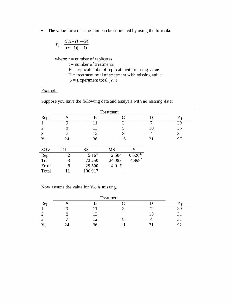
The value for a missing plot can be estimated by using the formula:
)1)(1(
)(
tr
GtTrBYij
where: r = number of replicates
t = number of treatments
B = replicate total of replicate with missing value
T = treatment total of treatment with missing value
G = Experiment total (Y..)
Example
Suppose you have the following data and analysis with no missing data:
Treatment
Rep A B C D Y.j
1 9 11 3 7 30
2 8 13 5 10 36
3 7 12 8 4 31
Yi. 24 36 16 21 97
SOV Df SS MS F
Rep 2 5.167 2.584 0.526ns
Trt 3 72.250 24.083 4.898*
Error 6 29.500 4.917
Total 11 106.917
Now assume the value for Y32 is missing.
Treatment
Rep A B C D Y.j
1 9 11 3 7 30
2 8 13 10 31
3 7 12 8 4 31
Yi. 24 36 11 21 92

Step 1. Estimate the missing value for Y32 using the formula:
5.7
)14)(13(
92)11*4()31*3(
)1)(1(
)(
tr
GtTrBYij
Step 2. Substitute the calculate value into the missing spot in the data.
Treatment
Rep A B C D Y.j
1 9 11 3 7 30
2 8 13 7.5 10 38.5
3 7 12 8 4 31
Yi. 24 36 18.5 21 99.5
Step 3. Complete the analysis.
Remember that you will loose one degree of freedom in error and total for each
missing value.
SOV Df SS MS F
Rep 2 10.792 5.396 1.023ns
Trt 3 60.063 20.021 3.795ns
Error 5 26.375 5.275
Total 10 97.229
Facts About the Missing Value Analysis
Use of the estimated value does not improve the analysis or supply additional
information. It only facilitates the analysis of the remaining data.
The Error MS calculated using the estimate of the missing value is a minimum. Use
of any other value but the one calculated would result in a larger value.
The TRT SS and Rep SS are biased values. Unbiased values can be calculated using
Analysis of Covariance.
The mean calculated using the estimate of the missing value is called a Least Square
Mean.
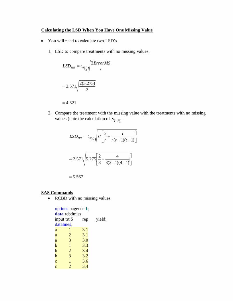
Calculating the LSD When You Have One Missing Value
You will need to calculate two LSD’s.
1. LSD to compare treatments with no missing values.
821.4
3
)275.5(2571.2
2
205.
r
ErrorMStLSDTRT
2. Compare the treatment with the missing value with the treatments with no missing
values (note the calculation of 21 YY
s
.
567.5
)14)(13(3
4
3
2275.5571.2
)1)(1(
22
205.
trr
t
rstLSDTRT
SAS Commands
RCBD with no missing values.
options pageno=1;
data rcbdmiss
input trt $ rep yield;
datalines;
a 1 3.1
a 2 3.1
a 3 3.0
b 1 3.3
b 2 3.4
b 3 3.2
c 1 3.6
c 2 3.4

c 3 3.6
d 1 3.9
d 2 4.0
d 3 4.2
;;
ods rtf file='rcbd nomiss.rtf';
proc anova;
class rep trt;
model yield=rep trt;
means trt/lsd;
title 'ANOVA for RCBD with no Missing Data';
run;
ods rtf close;
SAS commands for one missing data point
options pageno=1;
data rcbdmiss
input trt $ rep yield;
datalines;
a 1 3.1
a 2 3.1
a 3 3.0
b 1 3.3
b 2 .
b 3 3.2
c 1 3.6
c 2 3.4
c 3 3.6
d 1 3.9
d 2 4.0
d 3 4.2
;;
ods rtf file='rcbd nomiss.rtf';
proc glm;
class rep trt;
model yield=rep trt;
lsmeans trt/lsd;
title 'ANOVA for RCBD with Missing Data';
run;
ods rtf close;
SAS uses a period for missing data. Other
programs may use different values, such as a
dash (-) or -999.
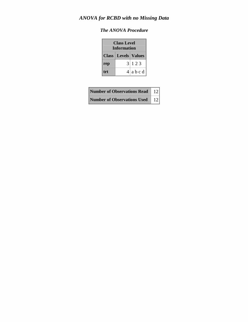
ANOVA for RCBD with no Missing Data
The ANOVA Procedure
Class Level
Information
Class Levels Values
rep 3 1 2 3
trt 4 a b c d
Number of Observations Read 12
Number of Observations Used 12

ANOVA for RCBD with no Missing Data
The ANOVA Procedure
Source DF
Sum of
Squares
Mean
Square F Value Pr > F
Model 5 1.53833333 0.30766667 18.77 0.0013
Error 6 0.09833333 0.01638889
Corrected Total 11 1.63666667
R-Square Coeff Var Root MSE yield Mean
0.939919 3.675189 0.128019 3.483333
Source DF Anova SS Mean Square F Value Pr > F
rep 2 0.00166667 0.00083333 0.05 0.9508
trt 3 1.53666667 0.51222222 31.25 0.0005

ANOVA for RCBD with no Missing Data
The ANOVA Procedure
Note
:
This test controls the Type I comparisonwise error rate, not the
experimentwise error rate.
Alpha 0.05
Error Degrees of Freedom 6
Error Mean Square 0.016389
Critical Value of t 2.44691
Least Significant Difference 0.2558
Means with the same letter
are not significantly different.
t Grouping Mean N trt
A 4.0333 3 d
B 3.5333 3 c
B
C B 3.3000 3 b
C
C 3.0667 3 a

ANOVA for RCBD with Missing Data
The GLM Procedure
Class Level
Information
Class Levels Values
rep 3 1 2 3
trt 4 a b c d
Number of Observations Read 12
Number of Observations Used 11

ANOVA for RCBD with Missing Data
The GLM Procedure
Dependent Variable: yield
Source DF
Sum of
Squares
Mean
Square F Value Pr > F
Model 5 1.55422980 0.31084596 20.76 0.0023
Error 5 0.07486111 0.01497222
Corrected Total 10 1.62909091
R-Square Coeff Var Root MSE yield Mean
0.954047 3.505134 0.122361 3.490909
Source DF Type III SS Mean Square F Value Pr > F
rep 2 0.01013889 0.00506944 0.34 0.7279
trt 3 1.55263889 0.51754630 34.57 0.0009
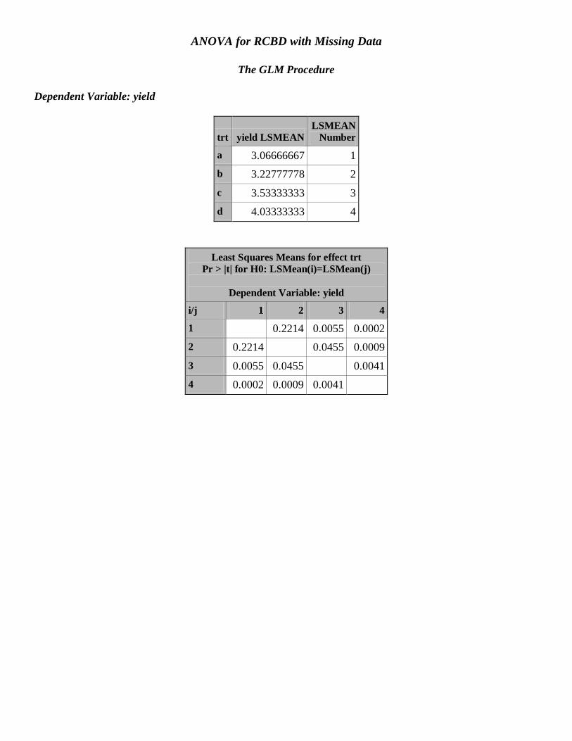
ANOVA for RCBD with Missing Data
The GLM Procedure
Dependent Variable: yield
trt yield LSMEAN
LSMEAN
Number
a 3.06666667 1
b 3.22777778 2
c 3.53333333 3
d 4.03333333 4
Least Squares Means for effect trt
Pr > |t| for H0: LSMean(i)=LSMean(j)
Dependent Variable: yield
i/j 1 2 3 4
1 0.2214 0.0055 0.0002
2 0.2214 0.0455 0.0009
3 0.0055 0.0455 0.0041
4 0.0002 0.0009 0.0041

RCBD with Sampling
As we had with the CRD with sampling, we will have a source of variation for
sampling error.
Calculation of the Experimental Error df is done the same way as if there was no
sampling.
Calculation of the Sampling Error df is done the same way as was done for the CRD
with sampling.
ANOVA Table
SOV Df F
Rep r-1 Rep MS/Expt. Error MS
Trt t-1 Trt MS/Expt. Error MS
Experimental Error (r-1)(t-1)
Sampling Error (rts-1)-(tr-1)
Total trs-1
Example using the Experimental Error MS as the Denominator of the F-test
Treatment
Rep Sample A B C
1 1 78 68 89
1 2 82 64 87
Y11.=160 Y21.=132 Y31.=176 Y.1.=468
2 1 74 62 88
2 2 78 66 92
Y12.=152 Y22.=128 Y32.=180 Y.2.=460
3 1 80 70 90
3 2 84 60 96
Y13.=164 Y23.=130 Y33.=186 Y.3.=480
Yi.. 476 390 542 Y…= 1408

Step 1. Calculate the Correction Factor (CF).
889.136,110)2)(3(3
140822
... rts
Y
Step 2. Calculate the Total SS:
111.2121
96...748278
2222
2
CF
CFYSSTotal ijk
Step 3. Calculate the Replicate SS.
778.33
)2(3
480
)2(3
460
)2(3
468
Rep
222
2
..
CF
CFts
YSS
j
Step 4. Calculate the Treatment SS:
444.1936
)2(3
542
)2(3
390
)2(3
476
222
2
..
CF
CFrs
YSSTreatment i

Step 5. Calculate the SS Among Experimental Units Total (SSAEUT)
111.2003
2
186...
2
164
2
152
2
160
2222
2
.
CF
CFs
YAEUTSS
ij
Step 6. Calculate the Experimental Error SS:
Experimental Error SS = SAEUT – SS TRT – SS REP
= 2003.111 – 1936.444 – 33.778
= 32.889
Step 7. Calculate the Sampling Error SS:
Sampling Error SS = Total SS – SSAEUT
= 2121.111 – 2003.111
= 118.0
Step 8. Complete the ANOVA Table:
SOV Df SS MS F
Rep r-1=2 33.778 16.889 2.054ns
Trt t-1 = 2 1936.444 968.222 117.76**
Experimental Error (r-1)(t-1) = 4 32.889 8.222
Sampling Error (trs-1) - (tr-1) = 9 118.0
Total trs-1 = 17 2121.111
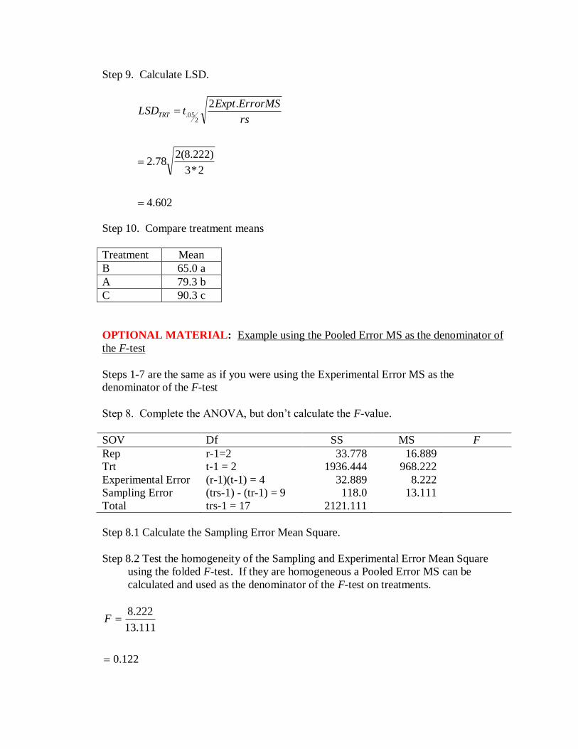
Step 9. Calculate LSD.
602.4
2*3
)222.8(278.2
.2
205.
rs
ErrorMSExpttLSDTRT
Step 10. Compare treatment means
Treatment Mean
B 65.0 a
A 79.3 b
C 90.3 c
OPTIONAL MATERIAL: Example using the Pooled Error MS as the denominator of
the F-test
Steps 1-7 are the same as if you were using the Experimental Error MS as the
denominator of the F-test
Step 8. Complete the ANOVA, but don’t calculate the F-value.
SOV Df SS MS F
Rep r-1=2 33.778 16.889
Trt t-1 = 2 1936.444 968.222
Experimental Error (r-1)(t-1) = 4 32.889 8.222
Sampling Error (trs-1) - (tr-1) = 9 118.0 13.111
Total trs-1 = 17 2121.111
Step 8.1 Calculate the Sampling Error Mean Square.
Step 8.2 Test the homogeneity of the Sampling and Experimental Error Mean Square
using the folded F-test. If they are homogeneous a Pooled Error MS can be
calculated and used as the denominator of the F-test on treatments.
122.0
111.13
222.8
F

Step 8.3 Look up the table F-value
This F-test is a one-tail test because there is the expectation that the Experimental
Error MS 22
ES s is going to be larger than the Sampling Error MS 2
S .
Thus, if you are testing = 0.01, then you need to use the F-table for α = 0.01.
F
))((,01.0 SampErrdfExptErrdf = F 422.69,4;01.0
Step 8.4 Make conclusions:
Since the calculated value of F (0.122) is less than the Table-F value (6.422), we
fail to reject Ho: Sampling Error MS = Experimental Error MS at the 99% level of
confidence.
Therefore, we can calculate a Pooled Error MS
Step 8.5: Calculate the Pooled Error df and the Pooled Error MS
Pooled Error df = Sampling Error df + Experimental Error df = (9+4) = 13
Pooled Error MS = Sampling Error SS + Experimental Error SS
Sampling Error df + Experimental Error df
= 607.1149
889.320.118
Step 9. Complete the ANOVA by calculating the F-value using the Pooled Error MS as
the denominator of the F-test.
SOV Df SS MS F
Rep r-1=2 33.778 16.889 1.455
Trt t-1 = 2 1936.444 968.222 83.417**
Experimental Error (r-1)(t-1) = 4 32.889 8.222
Sampling Error (trs-1) - (tr-1) = 9 118.0 13.111
Total trs-1 = 17 2121.111 11.607
Pooled Error 13 150.89
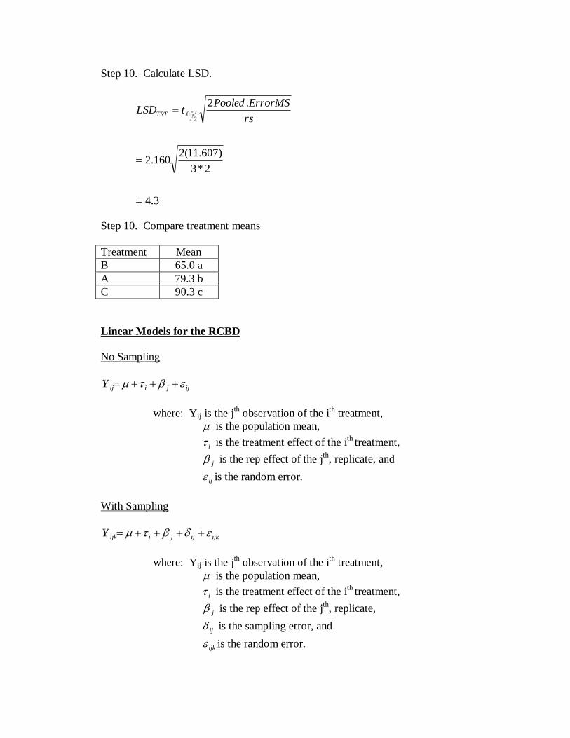
Step 10. Calculate LSD.
3.4
2*3
)607.11(2160.2
.2
205.
rs
ErrorMSPooledtLSDTRT
Step 10. Compare treatment means
Treatment Mean
B 65.0 a
A 79.3 b
C 90.3 c
Linear Models for the RCBD
No Sampling
ijjiijY
where: Yij is the jth observation of the i
th treatment,
is the population mean,
i is the treatment effect of the ith
treatment,
j is the rep effect of the jth
, replicate, and
ij is the random error.
With Sampling
ijkijjiijkY
where: Yij is the jth observation of the i
th treatment,
is the population mean,
i is the treatment effect of the ith
treatment,
j is the rep effect of the jth
, replicate,
ij is the sampling error, and
ijk is the random error.

Experimental Error in the RCBD
-The failure of treatments observations to have the same relative rank in all replicates.
Example 1
Treatments
Rep A B C D E
1 2 3 4 5 6
2 3 4 5 6 7
3 4 5 6 7 8
*Note that each treatment increases by one from replicate to replicate.
Example 2
Fill in the given table so the Experimental Error SS = 0.
Treatments
Rep A B C D E
1 2 6 1 8 4
2 4
3 1
4 5
Answer
Treatments
Rep A B C D E
1 2 6 1 8 4
2 4 8 3 10 6
3 1 5 0 7 3
4 5 9 4 11 7

SAS Commands for the RCBD With Sampling
options pageno=1;
data rcbdsamp;
input Rep Sample Trt $ yield;
datalines;
1 1 a 78
1 2 a 82
2 1 a 74
2 2 a 78
3 1 a 80
3 2 a 84
1 1 b 68
1 2 b 64
2 1 b 62
2 2 b 66
3 1 b 70
3 2 b 60
1 1 c 89
1 2 c 87
2 1 c 88
2 2 c 92
3 1 c 90
3 2 c 96
;;
ods rtf file='rcbdsamp.rtf';
proc anova;
class rep trt;
model yield=rep trt rep*trt;
test h=rep trt e=rep*trt;
means trt/lsd e=rep*trt;
title 'RCBD With Sampling Using the Experimental Error as the Error
Term';
run;
proc anova;
class rep trt;
model yield=rep trt;
means trt/lsd;
title 'RCBD With Sampling Using the Pooled Error as the Error Term';
Run;
ods rtf close;

RCBD With Sampling Using the Experimental Error as the Error Term
The ANOVA Procedure
Class Level
Information
Class Levels Values
Rep 3 1 2 3
Trt 3 a b c
Number of Observations Read 18
Number of Observations Used 18
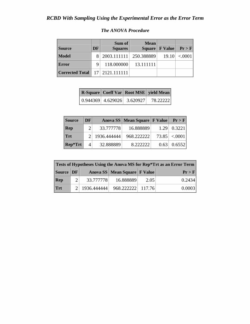
RCBD With Sampling Using the Experimental Error as the Error Term
The ANOVA Procedure
Source DF
Sum of
Squares
Mean
Square F Value Pr > F
Model 8 2003.111111 250.388889 19.10 <.0001
Error 9 118.000000 13.111111
Corrected Total 17 2121.111111
R-Square Coeff Var Root MSE yield Mean
0.944369 4.629026 3.620927 78.22222
Source DF Anova SS Mean Square F Value Pr > F
Rep 2 33.777778 16.888889 1.29 0.3221
Trt 2 1936.444444 968.222222 73.85 <.0001
Rep*Trt 4 32.888889 8.222222 0.63 0.6552
Tests of Hypotheses Using the Anova MS for Rep*Trt as an Error Term
Source DF Anova SS Mean Square F Value Pr > F
Rep 2 33.777778 16.888889 2.05 0.2434
Trt 2 1936.444444 968.222222 117.76 0.0003

RCBD With Sampling Using the Experimental Error as the Error Term
The ANOVA Procedure
t Tests (LSD) for yield
Note
:
This test controls the Type I comparisonwise error rate, not the
experimentwise error rate.
Alpha 0.05
Error Degrees of Freedom 4
Error Mean Square 8.222222
Critical Value of t 2.77645
Least Significant Difference 4.5965
Means with the same letter
are not significantly different.
t Grouping Mean N Trt
A 90.333 6 c
B 79.333 6 a
C 65.000 6 b
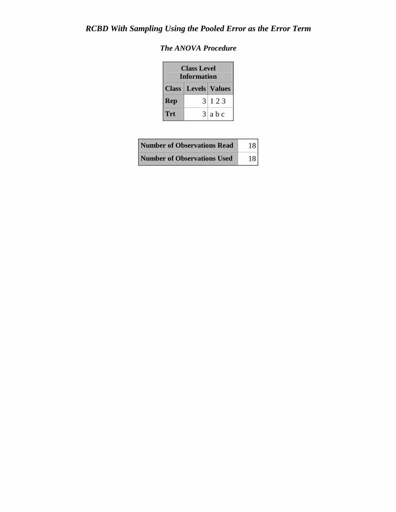
RCBD With Sampling Using the Pooled Error as the Error Term
The ANOVA Procedure
Class Level
Information
Class Levels Values
Rep 3 1 2 3
Trt 3 a b c
Number of Observations Read 18
Number of Observations Used 18
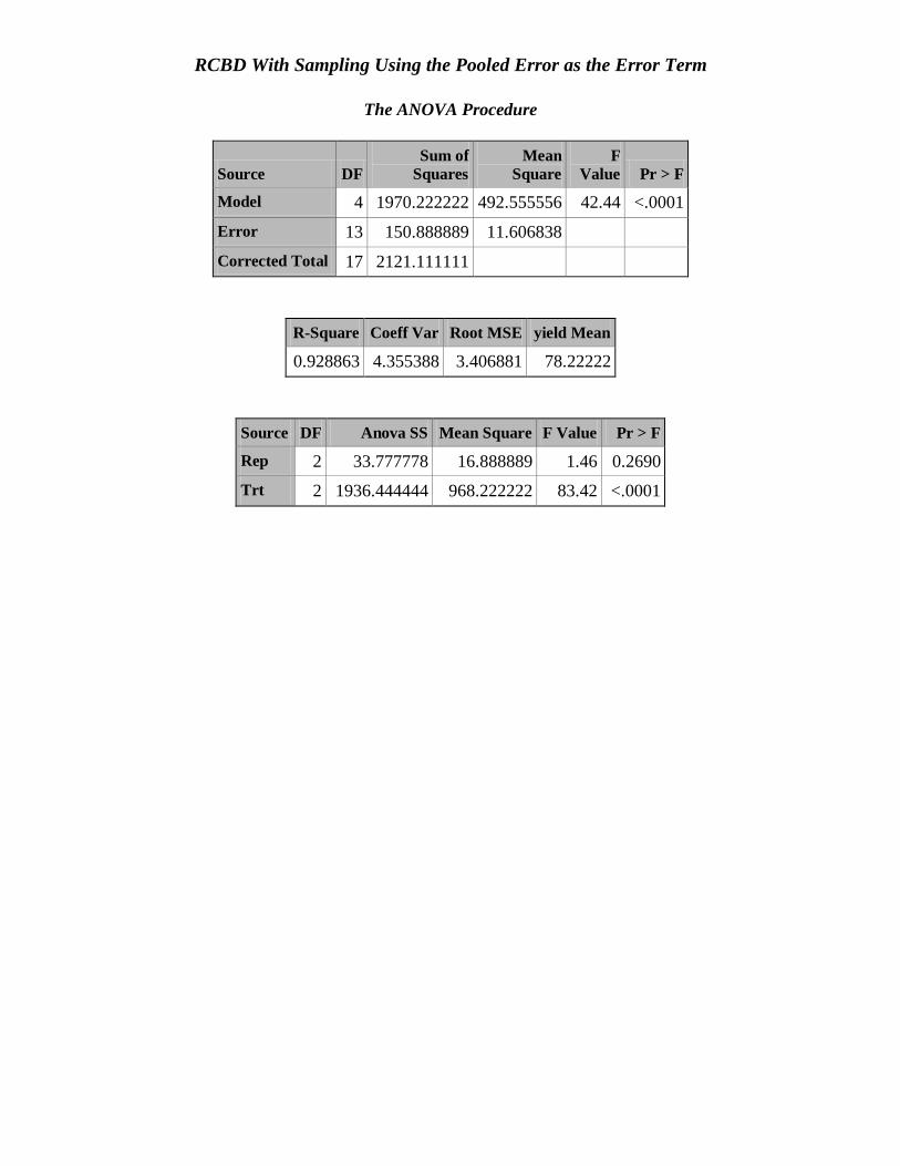
RCBD With Sampling Using the Pooled Error as the Error Term
The ANOVA Procedure
Source DF
Sum of
Squares
Mean
Square
F
Value Pr > F
Model 4 1970.222222 492.555556 42.44 <.0001
Error 13 150.888889 11.606838
Corrected Total 17 2121.111111
R-Square Coeff Var Root MSE yield Mean
0.928863 4.355388 3.406881 78.22222
Source DF Anova SS Mean Square F Value Pr > F
Rep 2 33.777778 16.888889 1.46 0.2690
Trt 2 1936.444444 968.222222 83.42 <.0001

RCBD With Sampling Using the Pooled Error as the Error Term
The ANOVA Procedure
t Tests (LSD) for yield
Note
:
This test controls the Type I comparisonwise error rate, not the
experimentwise error rate.
Alpha 0.05
Error Degrees of Freedom 13
Error Mean Square 11.60684
Critical Value of t 2.16037
Least Significant Difference 4.2494
Means with the same letter
are not significantly different.
t Grouping Mean N Trt
A 90.333 6 c
B 79.333 6 a
C 65.000 6 b


