Chapter 2

Random Sequences and StochasticProcesses

In this chapter we will begin with a formal definition of what a stochastic process is and how it canbe characterized. We will then study certain properties related to classes of processes which havesimple probabilistic characterizations both in terms of their so-called sample-path properties as wellas their probabilistic behavior. Throughout we will consider several ‘canonical’ examples which willaid us to better understand the concepts. We will conclude the chapter by seeing some of the mostimportant results in probability, the so-called limit theorems which are the Laws of Large Numbers(LLN’s both weak and strong) and the Central Limit Theorem. These results are powerful becauseof their generality and allow us to characterize the behavior of sequences and processes in large time.

2.1 Definitions and examples

Let (Ω,F , IP) be a probability space. Let T be an index set. For example T could be an arbitraryinterval in < or T = [a, b] × [c, d] a rectangle in <2 or T could be a discrete set such as the setof non-negative integers 0, 1, 2, .... Then the indexed family of r.v’s Xt(ω)t∈T is said to be astochastic process. This means that for each fixed t ∈ T , Xt(ω) defines a random variable. If T isan interval of < then Xt(ω) is said to be a continuous one-parameter stochastic process. Usually wethink of t as time and if T is continuous then the term continuous-time stochastic process is used.If t is a point inn a rectangle i.e. t = (t, s) ∈ [a, b] × [c, d] then Xt(ω) is a two-parameter stochasticprocess which is referred to as a random field. This can be extended to an arbitrary n-dimensionalindex set. If T is discrete we usually refer to the process as a discrete-parameter(or time) stochasticprocess. Discrete-time processes can be thought of as sequences of r.v’s. In these notes we willrestrict ourselves to the study of one-parameter stochastic processes in discrete as well as continuoustime. Without loss of generality we take X to be < or the process takes real values. The extension tovector-valued or <n valued processes is direct but it will simplify notation to consider the processesto be real valued.

As we have seen the mapping Xt(ω) : Ω → X where X denotes the space in which Xt takesits values is a random variable. On the other hand for every fixed ω ∈ Ω the mapping Xt(ω) asa function of t is called a realization or sample-path of the process. It is a deterministic functionof t. The problem is that we usually do not know ω and only have information on the underlyingprobabilities of joint events of the type Xti ∈ Ai available. From this we need to get a goodcharacterization of the process. This is what we discuss below. Also we drop the argument ω as

1

before.Let Tn = (t1, t2, ..., tn) be an arbitrary partition of T i.e. Tn denotes a finite collection of points in

T . Then Xt1 , ...,Xtn forms a collection of r.v’s which are characterized by their joint distribution

FTn = Ft1,..,tn(x1, x2, ..., xn)

The family of joint distributions Ftn for all finite partitions Tn of T is called the finite dimensionaldistributions of Xt. The joint distributions FTn are said to be compatible if they satisfy theproperty of consistency (given in Chapter 1) and symmetry (i.e. if we take any permutation of(t1, ..., tn) then the joint distribution remains the same). Now given a family of finite dimensionaldistributions there is the important theorem of Kolmogorov which states that these can be associatedwith the finite dimensional distributions of a stochastic process i.e. finite dimensional distributionsfor every finite partition are sufficient to characterize a stochastic process. This is stated belowwithout proof.

Theorem 2.1.1 (Kolmogorov extension theorem)Let FTn be a compatible family of finite dimensional distributions for Tn ∈ T . Then there

exists a probability space (Ω,F , IP) and a stochastic process Xt defined thereon such that the finitedimensional distributions of Xt coincide with FTn .

Let us study the implications of the theorem by the aid of two canonical examples. It is importantto note is that what the theorem states is the existence of a probability space and thus, given a metricspace with finite-dimensional distributions defined thereon then a probability measure need not bedefined on the space without further restrictions on the distributions.Example 1: (Continuous time ‘white noise’) Take as the space Ω the space C[0, T ] i.e. the spaceof continuous functions. Consider the finite dimensional distributions defined by:

FTn(x1, x2, ..., xn) =1

(2π)n2

n∏i=1

(∫ xi

−∞e−

y2i2 dyi

)

i.e. the joint distribution of n i.i.d. N(0,1) random variables. Then it is easy to see that FTn formsa compatible family. Hence by the Kolmogorov extension theorem there exists a probability spaceΩ′,F , IP) and a stochastic process Xt defined there on with distributions FTn . Let us show thatΩ′ 6= Ω = C[0, T ] i.e. Xt cannot be continuous in t and possess such finite dimensional distributions.To show this we will show that if Ω is taken as C[0, T ] then the probability measure will fail to besequentially continuous (re. Section 1, Chapter 1) and thus cannot be countably additive.

Consider the events An = ω : Xt > ε,Xt+ 1n≤ −ε. Then:

IP(An) =1

2π

(∫ ∞ε

e−x2

2 dx

)2

Now since by assumption we take Xt ∈ C[0, T ] it implies that the event Xt 6= Xt+ is null andhence:

0 = limn→∞

IP(An) =1

2π

(∫ ∞ε

e−x2

2 dx

)2

> 0

for all ε > 0 which leads to a contradiction and violates the sequential continuity of IP. HenceΩ′ 6= C[0, T ].

2

A natural question is what is the appropriate choice of Ω′?. The answer is that Ω′ can be takento be the space R[0,T ]. It turns out that this space is too large to yield any ‘nice’ properties for Xt.But it is beyond the scope of the course.Example 2: (Gaussian processes) The second example we consider is a discrete-time Gaussianprocess. The question is can we define a discrete-time Gaussian process on the space `2 which isthe space of square summable sequences i.e. `2 = xn :

∑∞n=1 |xn|

2 < ∞. Now if Xn is said tobe a discrete-time Gaussian process if the finite-dimensional distributions are Gaussian . Let Cn(h)denote the characteristic functional. For simplicity we consider the r.v’s to be zero mean. Then:

Cn(h) = E[eı∑n

i=1hiXi ] = e

− 12

∑n

i=1

∑n

j=1ri,jhihj

where ri,j = E[XiXj ] and hj are arbitrary scalars. Now suppose we consider the limit of Cn(h)as n → ∞. If it is a characteristic functional it must satisfy the properties outlined in Chapter 1.For this it is necessary and sufficient that

∑i

∑j |ri,j| <∞ since otherwise by suitable choice of hi

the sum will be infinite and the limit of the characteristic functionals will be 0 and thus we cannotdefine a discrete-time Gaussian process in `2. Thus for example we cannot define a discrete-timewhite noise process i.e. with ri,j = δi,j where δ is the Kronecker delta in `2. Discrete-time whitenoise is defined on <∞ or the space of real valued sequences and this space is quite well defined andcan be considered as the canonical space on which all sequences of discrete-time stochastic processesare defined. This basically means that we have no problem of defining the probability space fordiscrete-time processes with given finite dimensional distributions unlike the continuous time case.

The aim of the examples has been to show that given a family of finite dimensional distributionsthen the construction of the probability space imposes some restrictions on either the sample-pathsif we want to define Ω or if we fix Ω then it implies restrictions on the distributions. Henceforthwe will always assume that the process Xt is defined on a probability space (Ω,F , IP) and we willnot usually explicitly specify the space except that such a space and process could be defined by theextension theorem.

2.2 Continuity of Stochastic Processes

Let Xtt∈T be a continuous time stochastic process. Unlike the case of deterministic functions oft there are different types of continuity w.r.t t that can be defined. This is due to the fact thatin the probabilistic context a property holding almost surely is different in general than a propertyholding in the mean etc. This is also the case with continuity. We need these concepts in order todifferentiate between processes that might be continuous at a given point vs that which is continuousover the entire interval and the fact that jump processes (i.e. processes which have discontinuities atcertain points in time) satisfy weaker forms of continuity but are actually very different in behaviorfrom those which which have no discontinuities.

Definition 2.2.1 (Continuity in probability) A stochastic process Xt is said to be continuous inprobability at t if :

IP(|Xt+h −Xt| ≥ ε)h→0→ 0 ∀ε > 0 (2.2. 1)

Definition 2.2.2 (Continuity in p-th mean) A stochastic process Xt is said to be continuous innthe p-th mean at t if

E[|Xt+h −Xt|p]h→0→ 0 (2.2. 2)

3

Remark: In light of Markov’s inequality if a process is continuous in the p-th mean it is continuousin probability. From Lyapunov’s inequality we obtain that if a process is continuous in the p-thmean then it is continuous in the r-th mean for all r < p.

Definition 2.2.3 (Almost sure continuity) A stochastic process Xt is said to be almost surelycontinuous at t if:

IP(ω : limh→0|Xt+h −Xt| = 0) = 1 (2.2. 3)

In each of the above definitions if the property holds for all t ∈ T then we simply state that therespective continuity holds.

A final form of continuity which is the strongest is the notion of almost sure sample continuity.In order to define this we first need to define the notion of separability of a stochastic process.

Definition 2.2.4 (Separability) A stochastic process Xt is said to be separable if there exists acountable set S ∈ T such that for every interval I ∈ T and every closed set K ∈ < the events :

A = ω : Xt ∈ K, t ∈ I⋂T

andB = ω : Xt ∈ K, t ∈ S

⋂I

differ by a set Λ such that IP(Λ) = 0.

We state without proof that on a complete probability space we can always take Xt to be sep-arable. The importance of separability is the following: suppose we want to compute the probabilityof ω : suptXt ∈ A =

⋂t∈T ω : Xt ∈ A then such an set may not be measurable i.e. the resulting

set may not be an event since the intersection is over an uncountable intersection but if the processis separable then the intersection is taken over a countable set S and hence the resulting set is anevent due to the σ-algebra property of F and hence a probability can be defined.

Definition 2.2.5 (Almost sure sample continuity) A stochastic process Xt which is separable issaid to be almost surely sample continuous if :

IP(ω :⋃t∈T

limh→0|Xt+h −Xt| 6= 0) = 0 (2.2. 4)

Note almost sure continuity for every t does not imply almost sure sample continuity since ifit holds for every t then

⋃t∈T being an uncountable union need not be an event of probability 0

even if each is. It is difficult to characterize the event related to almost sure sample continuity interms of finite dimensional distributions of a process. However a sufficient condition for almost surecontinuity was given by Kolmogorov which we state without proof.

Proposition 2.2.1 (Kolmogorov criterion) Let Xtt∈T be a separable process and T be finite. Thena sufficient condition for Xt to be almost surely sample continuous is that there exist positiveconstants C,α, β such that :

E[|Xt+h −Xt|α] ≤ Ch1+β (2.2. 5)

4

Almost sure sample continuity implies almost sure continuity for every t. As mentioned we wouldlike to differentiate between processes which possess almost sure sample continuity from processeswhich are continuous everywhere except on a set of points t which are are finite but have o measurewith respect to the entire interval T i.e. Lebesgue measure 0. Such discontinuous processes are saidto possess discontinuities of the first kind if for every t the limits Xt+h and Xt−h exist as h→ 0 butare not equal. An example is right continuous processes for which Xt− 6= Xt. A sufficient conditionfor this is due to Cramer which we also give without proof.

Proposition 2.2.2 Let Xt be a separable process. Then with probability 1 every sample path ofXt has only discontinuities of the first kind if there exist positive constants C,α, β such that :

supt≤s≤t+h

E[|Xt+h −Xs|α|Xs −Xt|

α] ≤ Ch1+β (2.2. 6)

Remark: The Cramer’s condition is weaker than Kolmogorov’s criterion since by the Cauchy-Schwarz inequality we have that if Kolmogorov’s condition is satisfied with C,α, β then Cramer’scondition is satisfied with C, α2 , β.

Let us now consider some examples.Example 1: Let Xtt∈[0,T ] be A Gaussian process with mean 0 and :

E[|Xt+h −Xt|2] = h

Then it is easy to see that it is continuous in probability, in the quadratic mean (mean of order 2).Let us show that it is also almost surely sample continuous. For this note that since Xt+h −Xt

is Gaussian we have thatE[|Xt+h −Xt|

4] = 3h2

Therefor the process satisfies Kolmogorov’s criterion with C = 1, α = 4 and β = 1 and hence isalmost surely sample continuous. We shall study this process further later on. It is called a Wienerprocess.

Example 2: Let Ntt∈[0,∞) be a point process i.e. N0 = 0 and Nt takes values in the set of non-negative integers 0, 1, 2, ... with the following property : there exist a sequence of random timestn with t1 < t2 < t3 < ... such that at times tn Ntn = n and the process remains constant onthe interval [ti, ti+1) and for any s < t < u the random variables Nu − Nt and Nt − Ns are

independent with IP(Nt+h − Nt = k] = (λh)k

k! e−λh. Then it can be seen that Nt is continuousin probability and the mean. The process is not almost surely sample continuous since for anyfinite interval IP(Nt+T − Nt > 0) = e−λT > 0 and thus there exist points of discontinuity whereNt− 6= Nt. It however satisfies the Cramer’s criterion with α = 1 and β = 1 and C = 1 and thus hasdiscontinuities of the first kind almost surely on any finite interval. The process we have defined iscalled a Poisson process which we shall study later on.

2.3 Classification of Stochastic Processes

In this section we will study some special classes of stochastic processes some of which we will studyin detail. The idea is to study processes about which we can give general properties for membersof the class for their distributions and moments. Unless explicitly stated we will usually considercontinuous-time processes i.e. when the index set T is a subset of or equal to <.

5

One of the most commonly encountered stochastic processes is the so-called Gaussian processalready briefly introduced in Section 2.1.

Definition 2.3.1 (Gaussian processes) A stochastic process Xt is said to be a Gaussian processif its finite dimensional distributions are Gaussian i.e. given any finite partition Tnt1, t2, .., tn ofT then the random variables Xt1 ,Xt2 , ...,Xtn are jointly Gaussian with characteristic functional:

C(h) = E[eı[h,X]] = eı[h,m]− 12

[Rh,h] (2.3. 7)

where m is the vector of means i.e. m = col(m1, ...,mn) with mi = E[Xti ] and R the covariancematrix with entries Ri,j = cov(Xti ,Xtj ).

Remark: It is of course of interest to know on what space such processes are defined. Let T = [0, T ]and now consider a partition Tn of [0,T] with n going to infinity, t1 = 0, tn = T and supj |tj−tj−1| →0 then it can readily be seen that the above vectorial inner-products converge to integrals and thelimit of the characteristic functional is just:

C(h) = eı∫ T

0hsmsds− 1

2

∫ T0

∫ T0R(t,s)hshtdtds

where mt = E[Xt] and R(t, s) = cov(Xt,Xs). It can be shown but it is beyond the scope of the coursethat if we require the above characteristic functional to correspond to a characteristic functional ofcountably additive probability measure whose finite dimensional distributions are as above then wemust have

∫ T0

∫ T0 |R(t, s)|dtds <∞ (as in the example in Section 2.1). Thus with this condition we

have that the Gaussian process is defined on Ω = L2[0, T ] or the space of square-integrable functionson [0, T ]. If T = [0,∞) then the space is L2[0,∞) which is a little less interesting since on sucha space all functions must go to 0 as t → ∞ for the integrals to exist. We will usually considerGaussian processes on a finite time interval.

The next important class of stochastic processes is the class of stationary processes.

2.3.1 Stationary processes

Definition 2.3.2 A stochastic process Xt is said to be (strict-sense) stationary if for any finitepartition t1, t2, ..., tn of T the joint distributions Ft1,t2,..,tn(x1, x2, .., xn) are the same as the jointdistributions Ft1+τ,t2+τ,..,tn+τ (x1, x2, ..., xn) for any τ .

What the above definition states is that the joint distributions of the process or its shifted versionare the same. In light of the definition since the shift τ is arbitrary the index set T is taken to be(−∞,∞). We usually use the term stationary for strict-sense stationary. For stationary processesthe following properties hold:

Proposition 2.3.1 Let Xt be a stationary process. Then:

1. E[Xt] = m i.e. its mean is a constant not depending on t.

2. Let R(t, s) = cov(Xt, xs) then R(t, s) is of the form R(t, s) = R(|t− s|) i.e. it only depends onthe difference between t and s.

6

Proof:1)Let Ft(x) denote the one-dimensional distribution of Xt. Then,

mt = E[Xt] =

∫xdFt(x) =

∫xdFt+τ (x)

= mt+τ

and since by stationarity it holds for all τ it implies that mt cannot depend on t ot it is a constant.

2) Let us for convenience take m=0. Then:

R(t, s) = E[XtXs] =

∫xydFt,s(x, y)

=

∫xydFt−s,0(x, y) = R(t− s, 0)

=

∫xydF0,s−t(x, y) = R(0, s− t)

Hence we obtain thatR(t, s) = R(t− s, 0) = R(0, s− t)

or R(t, s) must be a function of the magnitude of the difference between t and s.

The above requirement of strict sense stationarity is usually too strong for applications. In thecontext of signal processing a weaker form of stationarity just based on the mean and covariance isvery useful. This is the notion of wide sense stationarity abbreviated as w.s.s.

Definition 2.3.3 A stochastic process Xt with E[|Xt|2] < ∞ is said to be wide sense stationaryor w.s.s. if the properties 1. and 2. above hold i.e.

1. E[Xt] = m

2. R(t, s) = R(|t− s|)

In a later chapter we will study further properties of w.s.s. processes. It is important to notethat w.s.s. does not imply strict sense stationarity. However, if Xt is a Gaussian process, sincethe finite dimensional distributions are completely specified by the mean and covariance, then thereverse implication holds.

We now introduce another class of stochastic processes of importance in applications.

2.3.2 Markov processes

Definition 2.3.4 A stochastic process Xt is said to be a Markov process (or simply Markov) iffor any partition t1, t2, ..., tn of T with t1 < t2 < . . . < tn the conditional distribution satisfies:

IP(Xtn ≤ xn/Xtn−1 = xn−1,Xtn−2 = xn−2, ...,Xt1 = x1

)= IP

(Xtn ≤ xn/Xtn−1 = xn−1

)(2.3. 8)

For simplicity we will assume that conditional densities are defined and we will denote the con-ditional densities by p(xn, tn/xn−1, tn−1). An immediate consequence of the definition of a Markovprocess is the property of the conditional independence of the ‘future’ and ‘past’ given the present.This can often be taken as the definition of Markov processes and is readily generalizable to randomfields or multi-parameter processes where there is no-natural definition of a causal or increasing flowof ‘time’.

7

Proposition 2.3.2 Let Xt be a Markov process. Then for any t0 < t1 < t2 we have:

p(x2, t2;x0, t0/x1, t1) = p(x0, t0/x1, t1)p(x2, t2/x1, t1)

Proof: First note that the joint density of Xt0 ,Xt1 and Xt2 can be written as:

pt0,t1,t2(x0, x1, x2) = p(x2, t2/x0, t0;x1, t1)p(x0, t0/x1, t1)pt1(x1)

Using the Markov property and the definition of the conditional density we have:

pt0,t1,t2(x0, x1, x2)

pt1(x1)= p(x0, t0;x2, t2/x1, t1) = p(x2, t2/x1, t1)p(x0, t0/x1, t1)

which establishes the conditional independence property of the ‘future’ and ‘past’ given the ‘present’.

From the definition of the Markov property by repeated application it is easy to see that thejoint density of Xt0 , ...,Xtn can be written as:

p(x0, t0;x1, t1; ...;xn, tn) = p(x0, t0)n∏k=1

p(xk, tk/xk−1, tk−1)

and hence the joint distribution of a Markov process is completely specified by the initial dis-tribution and the conditional distributions (1 step) which are obtainable from knowledge of thetwo-dimensional distributions of the process.

The above written in terms of the conditional distributions F (xn, tn/xn−1, tn−1) = IP(Xtn ≤xn/Xtn−1 = xn−1) can be written as:

F (x0, t0;x1, t1; ...;xn, tn) =

∫ x0

−∞

∫ x1

−∞..

∫ xn−1

−∞F (xn, tn/yn−1, tn−1)dF (yn−1, tn−1/yn−2, tn−2)

....dF (y1, t1/y0, t0)dF (y0, t0)

From the above observation that a Markov process is completely specified by its two-dimensionaldistributions we can pose the following question: given the two-dimensional distributions of a processwhat conditions must they satisfy in order that the process be Markov? The answer is that theymust satisfy the following consistency properties.

1. F (x, t) =∫∞−∞ F (x, t/y, s)dF (y, s)

2. For t0 < s < t

F (x, t/x0, t0) =

∫ ∞−∞

F (x, t/y, s)dF (y, s/x0, t0)

Property 1) will be satisfied by any two-dimensional distribution by the definition of conditionaldistributions. Property 2 is the more important one which specifies the Markov property and isknown as the Chapman-Kolmogorov equation.

Let us study the constraints imposed by the two properties through a commonly used example.Suppose we want to define a Markov process Xt which can take only two values −1, 1 with

the following properties:

1. IP(Xt = 1) = IP(Xt = −1) = 12 for all t.

8

2. For t ≥ s

IP(Xt = Xs) = p(t− s)

IP(Xt = −Xs) = 1− p(t− s)

with p(t) continuous and p(0) = 1.

Let us study the constraints it imposes on p(.).It is easy to see that Property 1 is always satisfied for all p(t) since :

IP(Xt = 1) =1

2= IP(Xt = 1/Xs = 1)IP(Xs = 1) + IP(Xt = 1/Xs = −1)IP(Xs = −1)

=1

2p(t− s) +

1

2(1− p(t− s)) =

1

2

Property 2 or the Chapman-Kolmogorov equation specifies that p(.) must satisfy:

p(t− t0) = p(t− s)p(s− t0) + (1− p(t− s))(1− p(s− t0))

for all t0 < s < t. Changing variables by setting t0 = 0 and t − s = τ we obtain that p(.) mustsatisfy:

p(s+ τ) = p(τ)p(s) + (1− p(τ))(1− p(s))

orp(s+ τ) = 2p(τ)p(s)− (p(τ) + p(s))

Substituting p(t) = 1+f(t)2 we obtain that f(t) must satisfy:

f(s+ τ) = f(s)f(τ)

and the only non-trivial solution is that f(t) = e−λt for λ > 0 and hence we obtain

p(t) =1 + e−λt

2

showing the constraints imposed by the Markov assumption.

An important sub-class of Markovian processes is the so-called processes with independent in-crements or simply independent increment processes.

Definition 2.3.5 A stochastic process Xtt∈[t0,∞) is said to be an independent increment process iffor any arbitrary collection of non-overlapping intervals (si, ti]; i = 1, 2, ..., n of [t0,∞) the incrementsXti −Xsi

ni=1 and Xt0 form a collection of independent random variables.

Proposition 2.3.3 Let Xtt∈[0,∞) be an independent increment process. Then Xt is a Markovprocess.

9

Proof: Let ti be a partition of [0,∞) with t1 < t2 . . . < tn. Then to show that Xt is Markov it issufficient to show that IP(Xtn ≤ x/Xt1 = x1, ...Xtn−1 = xn−1) = IP(Xtn ≤ x/Xtn−1 = xn−1). Firstnote that:

Xtn = Xtn −Xtn−1 +Xtn−1 = Xtn−1 + Vn

and by the independent increment property Vn is independent of Xti ; i = 1, 2, ..., n − 1. Therefore:

F (tn, xn/t1, x1; t2, x2, ..., tn−1, xn−1) = F (Vn ≤ xn − xn−1/t1, x1; t2, x2; .., tn−1, xn−1)

= FVn(x2 − x1)

by the independence of Vn and Xtin−1i=1 . Hence since the distribution of Xtn is completely deter-

mined from the distribution of Vn and the knowledge of Xtn−1 = xn−1 it follows that the process isMarkov.

A particular class of independent increment processes those with stationary independent incre-ments forms an important class of processes which occur frequently in applications.

Definition 2.3.6 A stochastic process Xtt∈[0,∞) is said to be a process with stationary independentincrements if the increments are independent and the distribution of Xt−Xs for t > s only dependson the difference t− s.

The means and variances of stationary independent increment processes have a particularlysimple form i.e. they are affine functions of t. We prove this result below.

Proposition 2.3.4 Let Xtt∈[0,∞) be a stationary independent increment process. Then :

1. E[Xt] = m0 +m1t where m0 = E[X0] and m1 = E[X1]−m0.

2. var(Xt) = σ20 + σ2

1t where σ20 = var(X0) and σ2

1 = var(X1)− σ20.

Proof: We will show 2) since the stationary independent increment property is used. The proof of1) follows in a similar way except that only the stationary increment property is needed. To simplifythe proof without loss of generality we take the mean to be 0. Note by the independent incrementproperty E[XtXs] = E[X2

s ] since

E[XtXs] = E[(Xt −Xs +Xs)Xs]

= E[(Xt −Xs)Xs] + E[X2s ]

= E[Xt −Xs]E[Xs] + E[X2s ]

= E[X2s ]

since the process is assumed to be zero mean. If the means are non-zero then it can be readily seencov(XtXs) = var(Xs).

Define: g(t) = var(Xt+u−Xu) which does not depend on u by the stationary increment property.Then:

g(t+ s) = var(Xt+s −X0) = var(Xt+s −Xs +Xs −X0)

= var(Xt+s −Xs) + var(Xs −X0)

= g(t) + g(s)

10

Noting that∂g(t+ s)

∂s= g′(s) =

∂g(t + s)

∂t= g′(t)

we obtain that g′(t) = g′(s) for all s and t or g′(t) = K for some constant K. Hence :

g(t) = Kt+K1

is the general solution. Noting that from the relation above taking t = s = 0 we obtain g(0) = 2g(0)it implies that K1 = 0. Also since g(1) = K we obtain that K = var(X1 −X0). Finally noting that

var(Xt) = var(Xt −X0 +X0) = g(t) + var(X0)

where we have used the independent increment property once again. The proof is then completedby noting that var(X1−X0) = E[X2

1 ]− 2E[X1X0] + E[X20 ] = E[X2

1 ]−E[X20 ] = var(X1)− var(X0).

Remark: From the above it is evident that independent increment processes are defined on [0,∞)since if T = (−∞,∞) then it is easy to see that such a process for any finite t is infinite and notwell defined.

In signal processing (especially linear estimation theory) it is enough to require that the incre-ments are uncorrelated and form a w.s.s. process. We give the definitions below:

Definition 2.3.7 1. A stochastic process Xt is said to be an uncorrelated increment process ifthe increments are uncorrelated i.e. for any t1 < t2 < t3

E[(Xt3 −Xt2)(Xt2 −Xt1)] = E[(Xt3 −Xt2)]E[(Xt2 −Xt1 ]

2. A stochastic process Xt is said to be an orthogonal increment process if E[(Xt3 −Xt2)(Xt2 −Xt1)] = 0.

Remark: If Xt is zero mean and uncorrelated increment then it is an orthogonal incrementprocess. If the increments in addition to being orthogonal are w.s.s. then we have a w.s.s orthogonalincrement process. Such processes occur in the study of spectral theory and will be discussedin Chapter 4. Note if the process is Gaussian then the process will have stationary independentincrements.

Let us now discuss some concrete examples of Markov and independent increment processes.Example 1: Consider the following discrete-time process Xn defined by:

Xn+1 = fn(Xn,Wn)

where Wn is an independent sequence of r.v’s and fn(., .) is a deterministic function. Then Xnis a Markov process. The proof is trivial.

Example 2: Let Yn be a sequence of independent identically distributed r.v’s. Then:

Xn =n∑k=1

Yk

is a stationary independent increment process. If the Yn are only an independent sequence butnot identically distributed then Xn will be an independent increment process. When the Yn’s are

11

i.i.d r.v’s which take integer values in the set −1, 1, Xn is called a random walk. This model is avery important model in applications.

The next two examples we will discuss in detail since such processes are very basic processes inthe study of stochastic processes.

Definition 2.3.8 (Brownian motion or Wiener process)A continuous-time stochastic process Wt; t ≥ 0 is said to be a Brownian motion or Wiener

process with parameter σ2 if:

1. W0 = 0

2. Wt is a Gaussian process with mean 0 and E[WtWs] = σ2 min(t, s).

If σ2 = 1 then the process is said to be standard Brownian motion.

From the definition of Brownian motion the following properties can easily be shown.

Proposition 2.3.5 Let Wtt∈T be a Brownian motion process. Then:

1. Every sample path of Wt is almost surely sample continuous in t.

2. Wt is a stationary independent increment process.

Proof: For convenience we will take Wt as a standard Brownian motion.The proof of 1) follows from the fact that since the process is Gaussian Xt+h −Xt is Gaussian

and hence :E[|Xt+h −Xt|

4] = 3h2

and hence Kolmogorov’s criterion for almost sure sample continuity is satisfied with α = 4 ,β = 1and c = 3.

To prove the stationary independent increment property it is sufficient to that the process hasorthogonal increments and then since the process is Gaussian it implies that the increments areindependent. Stationary increment property follows from the fact that E[(Wt−Ws)

2] = (t−s). Theproof of the orthogonal increment property follows by noting that for t > s:

E[(Wt −Ws)(Ws)] = E[WtWs]−E[W 2s ]

= s− s = 0

showing that the increments are orthogonal.

The reason that the Wiener process or Brownian motion is so special is that one can show (whichwe will do later) that any Gauss-Markov process can be considered as a ‘time-changed’ Brownianmotion. Gauss-Markov processes arise in the modeling of linear stochastic systems with noise and willbe discussed in the next section. Actually there is an important result due to Paul Levy which statesthat if a process is Gaussian with stationary independent increments then it must be a Brownianmotion process.

The analog of the Brownian motion process for processes with discontinuous trajectories is thePoisson process. This process plays a fundamental role in the study of processes with discontinuoustrajectories the so-called jump processes. We define this below.

12

Definition 2.3.9 (Poisson Process) A stochastic process Ntt∈[0,∞) is said to be a Poisson processwith intensity λ if Nt takes values in 0, 1, 2, . . . and

1. N0 = 0

2. For all s, t ∈ [0,∞) with t > s then Nt −Ns is a Poisson r.v. with mean λ(t− s) i.e.

IP(Nt −Ns = k) =(λ(t− s))k

k!e−λ(t−s)

3. Nt is an independent increment process.

In light of property 2 above it implies that Nt is a stationary, independent increment processwith purely discontinuous sample-paths. Let us study some properties associated with Poissonprocesses.

First, note by virtue of the definition E[Nt] = λt and cov(Nt,Ns) = λ(min(t, s)). Let Ti∞i=1

denote the jump times of Nt with T0 = 0 i.e.

Nt = n t ∈ [Tn, Tn+1)

Then by definition of Tn we can define Nt as:

Nt =∞∑n=1

1(Tn≤t)

in other words we can define the Poisson process through its jump times. Such a process is referredto as a point process since the occurrence of the ‘points’ Tn at which the process jumps by 1 allowus to completely specify the process. Let us now study some properties associated with the jumptimes.

First note that by definition Tn ≤ t ≡ Nt ≥ n. Let FTn(t) denote the distribution of Tn.Then for n ≥ 1:

FTn(t) = 1−n−1∑k=0

e−λt(λt)k

k!

and the density

pTn(t) = λe−λt(λt)n−1

(n− 1)!; n ≥ 1, t ≥ 0

= 0 otherwise

In particular for n = 1 we obtain that pT1(t) = λe−λt; t ≥ 0 or T1 is exponentially distributed. Fromthe stationary independent increment property it implies that Tn+1−Tn have the same distributionas T1 and thus the interarrival times Sn = Tn − Tn−1 of a Poisson process form a sequence of i.i.d.exponential mean 1

λ r.v’s.It can be readily seen that Nt is not almost surely sample continuous although it can be shown

that it is continuous in the mean square and almost surely for every t. To see this note that for anyfinite interval T we have:

IP(Nt+T 6= Nt) = IP(Nt+T −Nt > 0) = e−λT > 0

which shows that there are finite number of discontinuities in any finite interval of time with non-zero probability showing that the process is not almost-surely sample continuous. It can readily beverified that Nt satisfies Cramer’s criterion.

Analogous to the result of Levy for Wiener processes there is the result of Watanabe which statesthat if a point process has stationary independent increments then it must be Poisson.

13

2.4 Gauss-Markov Processes

As we have seen that by definition a Wiener process is both Gaussian and Markov. However thestationary independent increment property is special to the Wiener process. Gauss-Markov processesare very basic processes which arise in the modeling of noisy linear stochastic systems. Consider forexample the following process defined by:

Xk+1 = AkXk + Fkwk (2.4. 9)

where wk is a i.i.d. N(0, Im) sequence (i.e. discrete-time <m-valued Gaussian white noise) andX0 ∼ N(m0,Σ0) and Ak is a n× n matrix and Fk is a n×m matrix. It is easily seen that Xk isa Gauss-Markov sequence. Such models arise in signal processing and control applications.

It turns out that the covariance of Gauss-Markov processes has a very particular structure whichis both necessary and sufficient for a Gaussian process to be Markov. Let us study this issue in somedetail.

Let Xt be a Gauss-Markov process. Without loss of generality we take the process to be 0mean. Let R(t, s) = cov(Xt,Xs). Then we can state the following result.

Proposition 2.4.1 Let Xt be a Gaussian process with R(t, t) > 0 for all t. Then for Xt to beMarkov it is necessary that for all t > s > t0

R(t, t0) =R(t, s)R(s, t0)

R(s, s)(2.4. 10)

Proof: First note that by the Gaussian property we have:

E[Xt/Xs] =R(t, s)

R(s, s)Xs

Using the Markov property we have:

E[Xt/Xt0 = X0] =R(t, t0)

R(t0, t0X0 =

∫ ∞−∞

xdF (t, x/t0,X0)

=

∫ ∞−∞

R(t, s)

R(s, s)ydF (s, y/t0,X0)

=R(t, s)

R(s, s)

R(s, t0)

R(t0, t0)X0

where we have used the Chapman-Kolmogorov equation in the third step and the definition of theconditional mean of a Gaussian process. Hence comparing the l.h.s. and the r.h.s., since it is truefor all X0 we obtain:

R(t, t0) =R(t, s)R(s, t0)

R(s, s)

It can be shown that for the covariance to satisfy the above property the covariance R(t, s)must be of the form f(max(t, s))g(min(t, s)). It turns out that this condition is also sufficient for aGaussian process to be Markov. We show this below.

14

Proposition 2.4.2 Let Xt be a Gaussian process with R(t, t) > 0 for all t and R(t, s) is contin-uous for (s, t) ∈ T × T . Then for Xt to be Markov it is necessary and sufficient that

R(t, s) = f(max(t, s))g(min(t, s)) (2.4. 11)

If in addition the process is stationary then

R(t) = R(0)e−λ|t−s|; λ ≥ 0 (2.4. 12)

and in particular λ = −log(R(1)R(0) ).

Proof:Define

ρ(t, s) =R(t, s)√

R(t, t)√R(s, s)

Then ρ(t, s) satisfies:ρ(t, t0) = ρ(t, s)ρ(s, t0)

for all t ≥ s ≥ t0. Now by the continuity of ρ(t, s) and the assumption that R(t, t) > 0 for all t ∈ Twe see that ρ(t, t) = 1 and these two facts imply that ρ(t, s) 6= 0 for all t, s ∈ int T . Then since

ρ(t, s) = ρ(t,t0)ρ(s,t0) for all t > s > t0 we have that :

ρ(t, s) =α(t)

α(s)

for some α(t). If on the other hand t < s then we have

ρ(t, s) =α(s)

α(t)

Hence,

ρ(t, s) =α(max(t, s))

α(min(t, s))

Hence it implies that for t > s we have: f(t) = α(t)√R(t, t) and g(s) = 1

α(s)

√R(s, s) and this

completes the proof of the necessity.The proof of the sufficiency is based on the time-change property of Brownian motion. Consider

the case t > s. Define the following time

τ(t) =g(t)

f(t)

where for t > s we have R(t, s) = f(t)g(s). Then by the Cauchy-Schwarz inequality we obtain that :

R(t, s) ≤√R(t, t)

√R(s, s)

Hence,

f(t)g(s) ≤√f(t)g(t)f(s)g(s)

orτ(s) ≤ τ(t)

15

implying that τ(t) is monotone non-decreasing in t. Define the process:

Yt = f(t)Wτ(t)

then Yt is a Gauss-Markov process since W. is Gauss-Markov and τ(t) is an increasing function of t.Hence for t > s

E[YtYs] = f(t)f(s)τ(s) = f(t)g(s)

implying Yt is a Gauss-Markov process with the given covariance function.Finally if the process Xt is stationary then R(t, s) = R(t− s) and hence:

ρ(t+ s) = ρ(t)ρ(s)

for ρ(.) defined above. The only non-trivial solution to this equation is that :

ρ(t) = ceλt

Now noting that ρ(0) = 1 implying c = 1 and ρ(1) = R(1)R(0) = eλ we obtain that λ = log(R(1)

R(0) ). Once

again by Cauchy-Schwarz inequality noting that R(τ) ≤ R(0) for all τ we note R(1)R(0) ≤ 1 implying

λ ≤ 0. This completes the proof by noting that R(t) = R(0)ρ(t).

Similar results can be shown in the discrete-time case. We just state the results without proof.

Proposition 2.4.3 Let Xn be a stationary Gaussian sequence. Then in order that Xn beMarkov it is necessary and sufficient that the covariance satisfy:

Rn = R0ρ|n|; 0 < ρ < 1 (2.4. 13)

where ρ = e−log(

R1R0

).

2.5 Convergence of random variables

In applications we are often interested in the large-time behavior of a stochastic process. The studyof these issues is fundamentally related to convergence of sequences of r.v’s (in discrete-time) orconvergence of the process (in continuous-time). As in the case of continuity there are various formsof convergence, some stronger than others, associated with processes. In this section we discuss theconvergence concepts associated with sequences of r.v’s and illustrate by example that they are notequivalent. For continuous-time processes similar definitions hold and we work with partitions andthen show a ‘uniformity’ result in going to the limit as the partitions decrease to 0. First note thatfor each ω ∈ Ω Xn(ω) defines a deterministic sequence. Hence, we could study the convergence ofthe sequence for each ω as in the case of real sequences. This is called the point-wise convergenceproperty. This is however too strong and thus in the case of random sequences we would like tostudy the convergence taking account of the fact that we have a probability measure defined on Ω.This leads to the following notions:

Definition 2.5.1 (Convergence in probability) A sequence of r.v’s Xn is said to converge to ar.v. X in probability if :

limn→∞

IP(|Xn −X| ≥ ε) = 0

for any ε > 0.

16

As in the case of real sequences we do not often know a priori the limit X and so the convergencecan be studied by the Cauchy criterion or mutual convergence in probability i.e.

Proposition 2.5.1 A sequence Xn converges in probability if and only if it converges mutuallyin probability or the sequence is Cauchy in probability i.e.

limm→∞

supn≥m

IP(|Xn −Xm| ≥ ε)→ 0

for ε > 0.

Note mutual convergence can be equivalently stated as:

limn→∞

supm

IP(|Xn+m −Xn| ≥ ε)→ 0

Definition 2.5.2 (Convergence in th p.th. mean) A sequence of r.v’s Xn is said to converge inthe p-th mean (also referred to as LP convergence) to X if :

limn→∞

E[|Xn −X|p] = 0

Of particular importance in applications is the convergence in the mean of order 2 called meansquare convergence or convergence in the quadratic mean (q.m)

An immediate consequence of the Markov and Lyapunov inequalities is the following result.

Proposition 2.5.2 Let Xn be a sequence of r.v’s.

a) A necessary and sufficient condition for Xn to converge in the p-th mean is that it be Cauchyin the p-th mean.

b) If Xn converges in the p-th. mean then Xn converges in the r-th mean for 1 ≤ r ≤ p.

Definition 2.5.3 (Almost sure convergence)A sequence Xn is said to converge to X almost surely if

IP(ω : limn→∞

|Xn −X| 6= 0) = 0

Once again if we do not know the limit a priori a necessary and sufficient condition for a.s.convergence is that the sequence be Cauchy a.s.

A final and weak form of convergence is the notion of convergence in distribution.

Definition 2.5.4 (Convergence in distribution) A sequence Xn converges to X in distribution iffor every bounded continuous function f(.) the following holds:

E[f(Xn)] → E[f(X)] as n→∞

Convergence in distribution is equivalent to the convergence of the characteristic function. In par-ticular the above condition implies that the distribution Fn(x) of Xn converges to the distributionF (x) of X for each x which is a point of continuity of F (.).

In most applications we either require q.m. convergence or a.s. convergence. Before giving someexamples we first state the following result which establishes the relationships between the differentforms of convergence. We will use the notation Xn

a.s→ to denote convergence a.s. and so on.

17

Proposition 2.5.3 Let Xn be a sequence of r.v’s. Then the following relationships hold:

1. Xna.s→ X ⇒ Xn

P→ X

2. XnLP→ X ⇒ Xn

P→ X

3. XnP→ X ⇒ Xn

d→ X

4. Xnd→ C(a constant)⇒ Xn

P→ C

5. XnP→ X ⇒ ∃ a subsequenceXnk

a.s→ X

Proof: The implication 1 follows directly from the definitions while 2 follows from Lyapunov’sinequality. We will prove 3 and 4 only. The proof of 5 is technical and we will omit it.

Proof of 3. Let f(.) be bounded and continuous, let |f(x)| ≤ c and let ε > 0 and N be such thatPr(|X| > N) ≤ ε

4c . Choose δ such that |f(x)− f(y) ≤ ε2c for X| < N and |x− y| < δ. Then:

E[|f(Xn)− f(X)|] = E[|f(Xn)− f(X)|1[|Xn−X|<δ,|X|≤N ]]

+E[|f(Xn)− f(X)|1[|Xn−X|<δ,|X|>N ]]

+E[|f(Xn)− f(X)|1|Xn−X|≥δ]]

≤ε

2+ε

2+ 2cIP(|Xn −X| ≥ δ)

and the third term on the r.h.s. above goes to 0 as n→∞ by convergence in probability, hence for nsufficiently large we can make the r.h.s. smaller that 2ε establishing the convergence in distribution.

The proof of 4 follows from the fact that for n sufficiently large the probability distribution isconcentrated around a ball of radius ε around C. Therefore for n sufficiently large :

IP(|Xn −C| ≤ ε) ≥ 1− δ

or:IP(|Xn −X| ≥ ε) ≤ δ

establishing the convergence in probability.

We now consider some examples to show that the various forms of convergence are not equivalent.In the next section we will study applications of convergence in terms of the so-called weak and stronglaws of large numbers and ergodic theorems.Example 1: (Lp convergence does not imply a.s. convergence) Let Xn be a sequence of indepen-dent 0, 1 valued r.v’s with IP(Xn = 1) = 1

n and IP(Xn = 0) = 1− 1n .

Then Xn converges to 0 in Lp for all p > 0 since : E[|Xn|p] = 1n . However, it does not converge

a.s since taking the events An = Xn = 1 gives:

∞∑n=1

IP(An) =∞∑n=1

pn =∞

(by Borel-Cantelli lemma).

18

Example 2: (a.s. convergence does not imply L2 convergence). Let X be a r.v. uniformlydistributed in [0,1]. Define:

Yn = n if 0 ≤ Y ≤1

n= 0 otherwise

Then clearly as n→∞ Yn → 0 a.s. but : E[Y 2n ] = n which goes to ∞.

Let us conclude with a result concerning a.s. convergence of sequences. This result is the key toestablishing important ergodic theorems discussed in the next section.

Proposition 2.5.4 Let Xn be a sequence of r.v’s with E[|Xn|2] <∞. If∑∞n=1 E[|Xn|2] <∞ then

Xn → 0 almost surely as n→∞.

Proof: Define the event :An = ω : |Xn| ≥ ε

Then, by the Chebychev inequality:

IP(An) ≤E[|Xn|2

ε2

Therefore,∞∑n=1

IP(An) ≤1

ε2

∞∑n=1

E[|Xn|2] <∞

Hence, by the Borel-Cantelli lemma, the probability that An i.o. is 0 or |Xn| ≥ ε only for a finitenumber of n. Since ε > 0 is arbitrary it implies that Xn → 0 a.s.

2.6 Laws of large numbers and the Central Limit Theorem

Strong and weak laws and their generalization, the so called ergodic theorem for stationary randomprocesses are concerned with the problem of when we can infer the statistics of a process (or anappropriate function of it) by observing a single realization of the process. Typically the quantitieswe wish to estimate are means and variances. This is the basis for practical algorithms where we onlyobserve a single realization or sample-path and we do not have the opportunity to observe numerousindependent realizations (i.e. the basis of Monte-Carlo methods) to then calculate ensemble averages.The difference between weak and strong laws is that for the former the conclusion is in terms ofa result holding in probability while the latter is an almost sure property. An intermediate resultcorresponds to the property holding in the mean squared sense.

Before we prove the results we first point out some facts about characteristic functions whichwill be used in some of the proofs.

Note by definition, the characteristic function of a r.v. is the Fourier transform of the densityfunction if it exists. Hence, a natural question is can we know when a density exists if are giventhe characteristic function? The answer is, yes. It really is just a consequence of the Fourierinversion theorem and we state the result along with other results about characteristic functions inthe following proposition.

19

Proposition 2.6.1 (More about characteristic functions)Let φ(h) denote the characteristic function associated with a probability distribution F (·) defined

on < i.e.

φ(h) =

∫<eıhxdF (x)

Then the following results hold:

a) For any points a, b ∈ < with a < b at which F (x) is continuous:

F (b)− F (a) = limc→∞

1

2π

∫ c

−c

e−ıta − e−ıtb

ıtφ(t)dt

b) If∫∞−∞ |φ(t)|dt <∞, the distribution function F (x) possesses a density

F (x) =

∫ x

−∞p(y)dy

and

p(x) =1

2π

∫ ∞−∞

e−ıtxφ(t)dt

c) If φ(k)(0) exists then:

E|X|k <∞ if k is even

E|X|k−1 <∞ if k is odd

d) If X ∼ F (.) and E[|X|k] <∞ then

φ(h) =k∑j=0

E[Xj ]

j!= o(tk)

The proofs of these results follow from standard Fourier theory and the use of the Taylor expan-sion.

Proposition 2.6.2 (Weak law of large numbers (WLLN)) Let Xn be a sequence of i.i.d r.v.’swith E[|X1|] <∞ and E[X1] = m. Then

1

n

n∑k=1

XkP→ m

Proof: Let C(h) = E[eıhX1 ] denote the characteristic function of Xi. Then denoting Sn =∑n

1 Xk:

Cn(h

n) = E[eıh

Snn ] =

[C(h

n)

]nBut for each h:

C(h) = 1 + ıhm+ o(h) h→ 0

Hence:

Cn(h

n) =

(1 + ı

h

nm+ o(

1

n)

)n20

Hence as n→∞ we have :

limn→∞

Cn(h

n)→ eıhm

which corresponds to the characteristic function of a probability distribution concentrated at m orSnn converges in distribution to a constant m which in light of the previous section implies that Sn

n

converges to m in probability.

In the above result we assumed that the sequence was i.i.d. We can remove the i.i.d. restrictionprovided that we impose further conditions such as the existence of the second moments. In thiscase we do not even need stationarity of the sequence. We give the form of the WLLN below.

Proposition 2.6.3 (WLLN for dependent 2nd. order sequences)Let Xn be a sequence of r.v’s with E[|Xn|2] < ∞ for all n. Let mk = E[Xk] and r(j, k) =

cov(Xj ,Xk). Suppose that |r(j, k)| ≤ Cg(|j − k|) with g(k)→ 0 as k →∞ then :

1

n

n∑k=1

(Xk −mk)P→ 0

Proof: Define Sn =∑nk=1(Xk −mk). Then using the Chebychev inequality:

IP(|Snn| ≥ ε) ≤

∑nj=1

∑nk=1 |r(j, k)|

n2ε2

≤ C

∑|k|≤n−1 g(k)(1− |k|n )

nε2

≤ 2C

∑|k|≤n−1 g(k)

nε2

Now since g(k) → 0 as k → ∞ for all n ≥ N(δε2C−1) we have g(n) ≤ δε2C−1 and hence for alln ≥ N(δε2):

IP(|Snn| ≥ ε) ≤ 2C

∑N(δε2)k=1 g(k)

nε2+ 2δ

The first term on the r.h.s. can be made as small as possible since it is a finite sum divided byn→∞ hence for n ≥ N(δε2C−1) large we can make:

IP(|Snn| ≥ ε) ≤ 2δ

and δ can be chosen arbitrarily small and so we have established convergence in probability.

Let us note some implications of the WLLN. Consider a collection of i.i.d. r.v’s Xini=1 withE[xi] = m and var(Xi) = σ2. Let us define: Mn = Sn

n . Then by the WLLN Mn → m andvar(Mn) → 0. However we obtain very little information about the behavior of Sn. For example,the weak law states that Sn is about nm where m is the mean when n is large. How good is thisestimate on how large Sn is? We need much more precision. It turns out that we can say quite a lotabout the limiting distribution of Sn − nm for large n under the rather weak assumption that theXn’s have finite variance. This is the essence of the powerful Central Limit Theorem (CLT) whichwe state and prove below.

21

Proposition 2.6.4 (Central Limit Theorem) Let Xini=1 be a sequence of i.i.d. r.v’s with E[x2i ] <

∞. Define Sn =∑ni=1Xi. Then as n→∞:

IP

(Sn − nm

σ√n≤ x

)→ Φ(x)

where E[X1] = m and var(X1) = σ2 and Φ(x) denotes the standard normal distribution givenby:

Φ(x) =1√

2π

∫ x

−∞e−

y2

2 dy

Proof: Let φ(t) = E[eit(X1−m)]Then:

φn(t) = E[eit(

Sn−nm)

σ√n

)]

=

[φ(

t

σ√n

)

]nBut from the expansion for φ(t) we have:

φ(t) = 1−σ2t2

2+ o(t) as t→ 0

Hence:

φn(t) = [1−σ2t2

2σ2n+ o(

1

n)]n → e−

t2

2

as n→∞ for fixed t.But the rhs is just the characteristic function of a N(0, 1) r.v. Hence the result is established

since the above result implies convergence in distribution.

Remarks: The above version of the CLT assumes that the r.v’s are i.i.d. There are much moregeneral versions of the CLT which can be shown in the absence of the i.i.d. hypothesis. However,there are important observations to be made even in the i.i.d. case. First note that no matter whatthe distribution is or whether the r.v’s are continuous or discrete, the limiting distribution of Sn−nm

σ√n

is Gaussian. The CLT thus provides the justification in stating that the scaled (by the factor√n)

convolution of copies of a probability distribution (measure) can be approximated by a Gaussiandistribution. However, is this approximation valid at the level of densities? It is well known thatjust because two functions are ”close” their derivatives need not be and since the density is thederivative of the distribution function it should not necessarily follow that density of the scaled (by√N) sum should also be close to a Gaussian density.

We can indeed state such a result if we impose some more conditions on the random variables.This result is often referred to as a Local Limit Theorem which have been developed by Gnadenko,Korolyuk, Petrov, etc. We omit the proof. It relies more on Fourier analysis rather than probability.

Proposition 2.6.5 (Local limit theorem)Let Xini=1 be a collection of i.i.d. mean 0 and variance 1 random variables. Suppose that their

common characteristic function φ(.) satisfies:∫ ∞−∞|φ(t)|rdt <∞

22

for some integer r ≥ 3. Then a density pn(x) exists for the normalized sum Sn√n

for n ≥ r and

furthermore:

pn(x) =1√

2πe−

x2

2

(1 +O(

1

nr−1

2

)

)Remark: Actually the error term can be made more precise given that moments of order r ≥ 2exist under the assumption on the characteristic function.

The next ergodic theorem concerns the ergodic property holding in the mean squared sense. Wefirst state the result for w.s.s. processes.

Proposition 2.6.6 a) Let Xn be a w.s.s. sequence of r.v’s with mean E[Xn] = m and covarianceR(k) = cov(Xn+k,Xn). Then

limn→∞

1

n

n−1∑k=0

R(k) = 0⇔

∑n−1k=0 Xk

n

L2

→ m

b) If Xt is q.m. continuous w.s.s. process with E[Xt] = m and covariance R(t) = cov(Xs+t,Xs).Then

limT→∞

1

T

∫ T

0R(t)dt = 0⇔

1

T

∫ T

0Xsds

L2

→ m

Proof: We prove a). The proof of b) is analogous. Proof of sufficiency: Define Sn =∑n−1k=0(Xk−m).

Then:

E[|Snn|2] =

1

n2

n−1∑k=0

n−1∑m=0

R(k −m)

=1

n

∑|k|≤n−1

R(k)(1−|k|

n)

Now from the non-negative definiteness of R(k) (see Chapter 3) it implies that∑n−1i=0

∑n−1j=0 R(i−j) =∑

|k|≤n−1R(k)(n− |k|) ≥ 0 implying that∑|k|≤n−1 nR(k) ≥

∑|k|≤n−1 |k|R(k) we obtain

1

n

∑|k|≤n−1

R(k)(1−|k|

n)n→∞→ 0

from which the sufficiency follows.The proof of the necessity follows from the fact that by the w.s.s. property:

|1

n

n−1∑k=0

R(k)| = |E[1

n

n−1∑k=0

(Xk −m)(X0 −m)]|

≤

√√√√E[(1

n

n∑k=0

(Xk −m))2]√

E[(X0 −m)2]

n→∞→ 0

Remark: If we remove the hypothesis that the process is w.s.s. but only retain the fact

that it is a second order process then a sufficient condition for 1n

∑n−1k=0(Xk − mk)

L2

→ 0 is that

23

1n2

∑n−1i=0

∑n−1j=0 R(i, j) → 0 as n → ∞. For the analogous result in for q.m. continuous processes is

that 1T 2

∫ T0

∫ T0 R(t, s)dtds→ 0 as T →∞.

We now discuss the SLLN (Strong Law of Large Numbers) and its generalization the individualergodic theorem for strictly stationary processes due to Birkhoff. We will omit the proofs since theyare technical but just indicate the fact that the SLLN follows from the Borel-Cantelli lemma. Asabove we state the SLLN for the case of non-stationary second-order processes and sequences dueto Cramer.

Proposition 2.6.7 (Strong Law of Large Numbers (SLLN))

a. Let Xn be a second order sequence with mean E[Xk] = mk and covariance R(j, k). SupposeR(j, k) satisfies for |j − k| large:

|R(j, k)| ≤ Cg(|j − k|)

such that1

n

∑|k|≤n−1

g(k)(1 −|k|

n) ≤

C

nα;α > 0

Then,

1

n

n−1∑k=0

(Xk −mk)a.s→ 0

b. Let Xt be a q.m. continuous process with E[Xt] = mt and covariance R(t, s). If for large|t− s|

|R(t, s)| ≤ Cg(|t− s|)

with1

T

∫ T

0g(t)(1 −

|t|

T)dt ≤

c

T γ; γ > 0

Then:1

T

∫ T

0(Xs −ms)ds

a.s.→ 0

Proof: We will prove this result under a more restrictive assumption, namely that Xn is a w.s.s.sequence with

∑∞k=0 |R(k)| <∞. This satisfies hypothesis a) with α = 1 and also the hypothesis of

the Proposition 2.6.6. Hence it follows that Snn → m in q.m. where E[Xn] = m and Sn =

∑nk=1Xk.

Since it converges in L2 it follows from Proposition 2.5.3 that ∃ a subsequence Sni such thatSnini→ m

a.s.Indeed let us choose ni = i2, then:

Pr|Si2

i2−m| > ε ≤

∑i2

1

∑i2

1 R(|j − k|)

i4ε2

≤2

i2ε2

i2−1∑k=0

|R(k)| ≤2

i2ε2

∞∑k=1

|R(k)|

Therefore:∞∑i=1

Pr|Si2

i2−m| > ε ≤

2∑∞k=0 |R(k)|

ε2

∞∑i=1

1

i2<∞

24

Hence, by the Borel-Cantelli lemma,Si2i2→ m a.s.

Now, let us assume that Xk is a non-negative sequence. This means that Sn increases with n.Hence, for i2 < n < (i+ 1)2 we have:

Si2

(i+ 1)2≤Snn≤S(i+1)2

i2

and noting that (i+1)2

i2→ 1 as i→∞ and the observation about

Si2i2

above we have

m ≤ limn→∞

Snn≤ m

and hence Snn → m a.s. as n→∞.

We extend the result to general Xn by noting that:

Xn = X+n −X

−n

where X=n = max(Xn, 0) and X−n = −min(Xn, 0) and so both X=

n and X−n are non-negative withE[Xn] = E[X+

n ] − E[X−n ]. By definition of X+n and X−n we have X+

n ≤ |Xn| and hence E|X+n |

2 ≤E|Xn|2. Similarly for X−n . Therefore E|X=

n |2 <∞ and E|X−n |

2 <∞ if E|Xn|2 <∞. Applying theresult for non-negative Xn to X+

n and X−n we have:

Snn

=

∑nk=1X

+k

n−

∑nk=1X

−k

n

and the result follows.

Remark: Condition b) holds if

|R(t, s)| <K

1 + |t− s|γ

for some constant K.

Let us conclude this section with a statement of the ergodic theorem for strictly stationaryprocesses. We will only discuss the continuous time case. The discrete-time case follows mutatismutandis.

Definition 2.6.1 A set A is said to be invariant for a process Xt if Xs ∈ A; s ∈ < implies thatXt+s ∈ A; s ∈ < for all t ∈ <. In other words the shifted version of the process remains in A.

An example of an invariant set is :

A = X. : limT→∞

1

T

∫ T

0f(Xs+t)dt = 0

Another example of a set which is not invariant the following:

A = X. : Xs ∈ (a, b) for some s ∈ [0, T ]

Then:

Definition 2.6.2 A stochastic process Xt is said to be ergodic if every invariant set A of realiza-tions is such that IP(A) = 0 or IP(A) = 1.

25

Remark: An ergodic process need not be stationary. For example a deterministic process can beergodic but is not stationary.

If the process is strictly stationary the following theorem can be stated.

Proposition 2.6.8 Let Xt be a strictly stationary process and f(.) be a measurable function suchthat E[|f(Xt)|] <∞. Then

a) The following limit :

limT→∞

1

T

∫ T

0f(Xs)ds

exists almost surely and is a random variable whose mean is E[f(X0)].

b) If in addition the process is ergodic then:

1

T

∫ T

0f(Xs)ds

a.s.→ E[f(X0)]

Let us study the issue of ergodicity a bit further via an example. The ergodic theorems (WLLN,

SLLN) state that time averages of the form either Snn or

∫ T0Xsds

T converge to their means or ensembleaverages E[X0] under appropriate conditions.

Ergodicity is much stronger since it states that limN→∞∑N−1k=0 f(Xk)→ E[f(X0)] for all ”nice”

functions. In other words, the SLLN applies to the sequence Yn = f(Xn). If we do not know thatXk is ergodic then we would have to check that the SLLN applies to Yk.

To do so let us consider the following example in continuous time for simplicity.Consider the process:

Xt(ω) = A(ω) cos(2πt+ θ(ω))

where A and θ are independent r.v’s with θ uniformly distributed in [0, 2π].Then one can show that Xt is strictly stationary (see Problem 6 at the end of the chapter). A

natural question is whether Xt is ergodic.First note that:

E[Xt] = E[A]

(1

2π

∫ 2π

0cos(2πt+ x)dx

)= 0

= E[X0]

since the integral of a cosine function over a period is 0.Also:

limT→∞

1

T

∫ T

0Xtdt = lim

T→∞

1

T

∫ T

0A cos(2πt+ θ)dt

= 0

Note, in the above A(ω) and θ(ω) are just treated as some constants. Hence the SLLN holds forXt(ω).

Now let us see if the result holds for any arbitrary but ”nice” function. Let f(.) be a continuousbounded function.

26

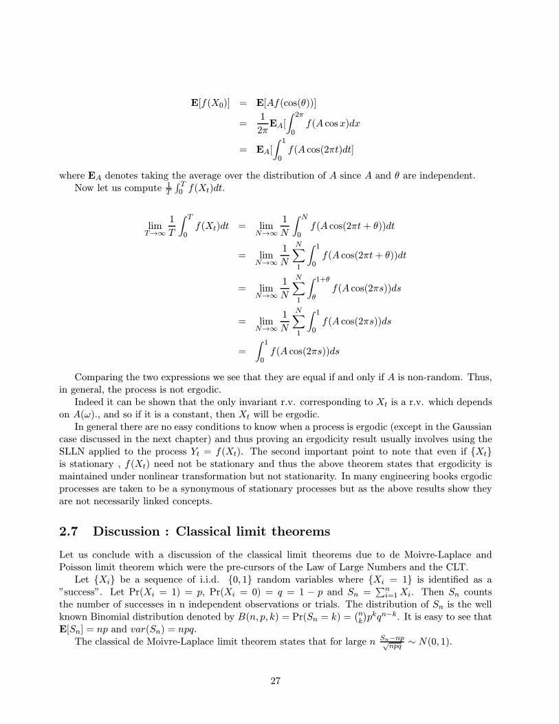
E[f(X0)] = E[Af(cos(θ))]

=1

2πEA[

∫ 2π

0f(A cosx)dx

= EA[

∫ 1

0f(A cos(2πt)dt]

where EA denotes taking the average over the distribution of A since A and θ are independent.Now let us compute 1

T

∫ T0 f(Xt)dt.

limT→∞

1

T

∫ T

0f(Xt)dt = lim

N→∞

1

N

∫ N

0f(A cos(2πt+ θ))dt

= limN→∞

1

N

N∑1

∫ 1

0f(A cos(2πt+ θ))dt

= limN→∞

1

N

N∑1

∫ 1+θ

θf(A cos(2πs))ds

= limN→∞

1

N

N∑1

∫ 1

0f(A cos(2πs))ds

=

∫ 1

0f(A cos(2πs))ds

Comparing the two expressions we see that they are equal if and only if A is non-random. Thus,in general, the process is not ergodic.

Indeed it can be shown that the only invariant r.v. corresponding to Xt is a r.v. which dependson A(ω)., and so if it is a constant, then Xt will be ergodic.

In general there are no easy conditions to know when a process is ergodic (except in the Gaussiancase discussed in the next chapter) and thus proving an ergodicity result usually involves using theSLLN applied to the process Yt = f(Xt). The second important point to note that even if Xtis stationary , f(Xt) need not be stationary and thus the above theorem states that ergodicity ismaintained under nonlinear transformation but not stationarity. In many engineering books ergodicprocesses are taken to be a synonymous of stationary processes but as the above results show theyare not necessarily linked concepts.

2.7 Discussion : Classical limit theorems

Let us conclude with a discussion of the classical limit theorems due to de Moivre-Laplace andPoisson limit theorem which were the pre-cursors of the Law of Large Numbers and the CLT.

Let Xi be a sequence of i.i.d. 0, 1 random variables where Xi = 1 is identified as a”success”. Let Pr(Xi = 1) = p, Pr(Xi = 0) = q = 1 − p and Sn =

∑ni=1Xi. Then Sn counts

the number of successes in n independent observations or trials. The distribution of Sn is the wellknown Binomial distribution denoted by B(n, p, k) = Pr(Sn = k) =

(nk

)pkqn−k. It is easy to see that

E[Sn] = np and var(Sn) = npq.The classical de Moivre-Laplace limit theorem states that for large n Sn−np√

npq ∼ N(0, 1).

27

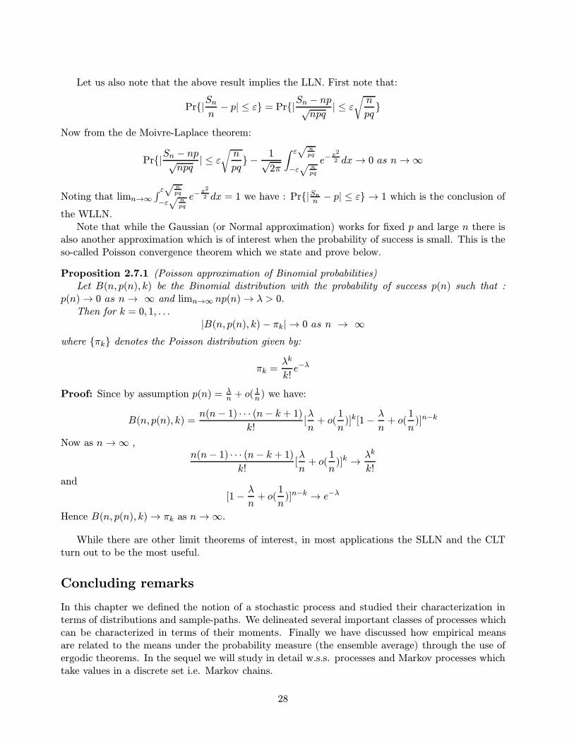
Let us also note that the above result implies the LLN. First note that:

Pr|Snn− p| ≤ ε = Pr|

Sn − np√npq

| ≤ ε√n

pq

Now from the de Moivre-Laplace theorem:

Pr|Sn − np√npq

| ≤ ε√n

pq −

1√

2π

∫ ε√

npq

−ε√

npq

e−x2

2 dx→ 0 as n→∞

Noting that limn→∞∫ ε√ n

pq

−ε√

npq

e−x2

2 dx = 1 we have : Pr|Snn − p| ≤ ε → 1 which is the conclusion of

the WLLN.Note that while the Gaussian (or Normal approximation) works for fixed p and large n there is

also another approximation which is of interest when the probability of success is small. This is theso-called Poisson convergence theorem which we state and prove below.

Proposition 2.7.1 (Poisson approximation of Binomial probabilities)Let B(n, p(n), k) be the Binomial distribution with the probability of success p(n) such that :

p(n)→ 0 as n→ ∞ and limn→∞ np(n)→ λ > 0.Then for k = 0, 1, . . .

|B(n, p(n), k) − πk| → 0 as n → ∞

where πk denotes the Poisson distribution given by:

πk =λk

k!e−λ

Proof: Since by assumption p(n) = λn + o( 1

n ) we have:

B(n, p(n), k) =n(n− 1) · · · (n− k + 1)

k![λ

n+ o(

1

n)]k[1−

λ

n+ o(

1

n)]n−k

Now as n→∞ ,n(n− 1) · · · (n− k + 1)

k![λ

n+ o(

1

n)]k →

λk

k!and

[1−λ

n+ o(

1

n)]n−k → e−λ

Hence B(n, p(n), k)→ πk as n→∞.

While there are other limit theorems of interest, in most applications the SLLN and the CLTturn out to be the most useful.

Concluding remarks

In this chapter we defined the notion of a stochastic process and studied their characterization interms of distributions and sample-paths. We delineated several important classes of processes whichcan be characterized in terms of their moments. Finally we have discussed how empirical meansare related to the means under the probability measure (the ensemble average) through the use ofergodic theorems. In the sequel we will study in detail w.s.s. processes and Markov processes whichtake values in a discrete set i.e. Markov chains.

28

Exercises

1. Let Xt be a random telegraph process defined as follows.

(a) Xt takes values −1, 1.

(b) IP(X0 = 1) = IP(X0 = −1) = 12

(c) Xt = (X0)(−1)Nt where Nt is a Poisson process with intensity λ > 0.

Find E[Xt], var(Xt) and cov(Xt,Xs). Show that it is an independent increment process.

2. Let Xt be a 0 mean Gaussian process with covariance

R(t, s) = exp−2λ|t− s|

Find the conditional density pXt/Xs(x/y). Show that it is not an independent incrementprocess.

3. Let Xt be the stochastic process defined below:

Xt =√

2cos(2πft+ φ)

where f and φ are random variables with the following densities:

pφ(φ) =1

2π0 ≤ φ ≤ 2π

pf (f) =2λ

λ2 + π2f2−∞ < f <∞

Find E[Xt] and cov(Xt,Xs).

The above problems show that there is very little information about a stochastic processobtained by knowing the mean and covariance without specifying the sample-paths.

4. Show that a Poisson process is mean square continuous and almost surely continuous at everyt.

5. Let Xt be a Gaussian process for t ∈ [0, T ]. Let E[|Xt+h−Xt|2] = hα for some α > 0. Showthat Xt is almost surely sample continuous no matter how small α can be.

6. Let Xt; −∞ < t <∞ be the stochastic process defined by:

Xt = A cos(2πt+ θ)

where A is a non-negative r.v. independent of θ which is uniformly distributed in [0, 2π).

(a) Show that Xt is a stationary process.

(b) Show that E[Xt] = 0 provided E[A] <∞.

(c) If A has the Rayleigh distribution given by:

pA(x) =x

σ2exp−

x2

2σ2 ;x ≥ 0

Show that Xt is a Gaussian process. Is Xt Markov?

29

7. a) Show√λW t

λis a standard Brownian motion process.

b) Let Xt; −∞ < t <∞ be a 0 mean Gaussian process with E[XtXs] = e−λ|t−s|. ExpressXt for t ≥ 0 in the form

Xt = f(t)W g(t)f(t)

where Wt; t ≥ 0 is a standard Brownian motion.

8. Consider the finite sequence of mean 0 jointly Gaussian r.v’s Xi10i=1 with:

E[XiXj ] = 2−|i−j|

Find:

a) E[X5/X4,X3]

b) E[X7/X8,X9,X10]

c) E[X6X9/X7,X8]

9. Let Nt; t ≥ 0 be a non-homogeneous Poisson process with time-dependent intensity λt > 0for all t defined as follows:

a) N0 = 0

b) For t > s, IP(Nt −Ns = k) =(∫ tsλudu)k

k! exp−∫ ts λudu

Show that Nt has independent increments. Let Tn be the points of Nt i.e. Nt = n; t ∈[Tn, Tn+1). Find the probability density pTn(t) and show that

∑∞n=1 pTn(t) = λt . Show that

IP(T1 <∞)) = 1⇒∫∞0 λudu =∞.

10. Let Xn be the discrete-time Gauss Markov process defined by:

Xn+1 = aXn + bwn

where X0 ∼ N(0, σ2) and wn is an i.i.d. N(0, 1) sequence independent of X0. DefineRk = E[X2

k ].

a) Show that Xn converges asymptotically to a stationary process if Rk → R∞ as n→∞.

b) Show that Rn → R∞ if |a| < 1. Find R∞.

c) Under the condition above, find what σ2 must be in order that Xn is a stationary process.

d) If a > 1 show that Xnan converges in the mean square.

11. Let Xn be a sequence of non-negative identically distributed r.v’s with E[Xn] < ∞. Thenshow that :

Xn

n

a.s→ 0

12. Let Nt be a Poisson process with intensity λ. Show that

Nt

t

a.s→ λ

30

13. Let Xn be i.i.d. r.v’s with mean m and finite variance. Define Sn =∑n

1 Xk. Then showthat:

E[X1/Sn, Sn+1, ...]a.s→ m

14. Let Xt be a zero mean w.s.s. process with covariance R(t). Suppose that for some T > 0,R(T ) = R(0). Then :

a) Show that IP(Xt+T = Xt) = 1 for every t.

b) Show that R(t+KT ) = R(t) for every t and not just for t=0.

c) Find the best linear mean squared estimate of Xt+KT given Xt i.e. find the constant Cwhich minimizes E[(Xt+KT − CXt)

2].

15. Let Xn be a second order sequence (mean 0). Show that a necessary and sufficient conditionfor Xn to converge in the mean square is that:

E[XnXm]→ C

as n,m →∞ independently and C is a constant. Using this condition repeat problem 10.

16. Let Xn be a sequence of independent 0, 1 r.v’s with Pr(Xn = 1) = pn and Pr(Xn = 0) =1− pn. Show that as n→∞

(a) XnP→0 ⇐⇒ pn → 0

(b) XnLp→ 0 ⇐⇒ pn → 0

(c) Xna.s.→ 0 ⇐⇒

∑∞n=1 pn <∞

17. Let us now consider some applications of the Chebychev inequality and the CLT in obtainingso-called sample size estimates in random sampling situations.

Let p be the fraction of a population who have a preference for a given product (or candidate).We choose n randomly sampled members of the population. Let Mn be the fraction of thesampled population who have the preference. Mn is thus an estimate of p.

a) Using Chebychev’s inequality and the fact that p(1−p) ≤ 0.25 find the size of the populationn if we want to obtain an estimate of p within 0.01 with 95% confidence.

b) Via the CLT show that a better estimate (smaller n) of the sample size is possible for thesame level of confidence.

Bibliography

The material for this section can be found in any standard text on stochastic processes. However,the following list of books may be consulted for more details (particularly 1 and 2).

1. E. Wong and B. Hajek; Stochastic processes in engineering systems, Springer-Verlag, N.Y., 1985

2. H. Cramer and M. R. Leadbetter; Stationary and related stochastic processes, J. Wiley and Sons,1967

31

3. W. B. Davenport and W. L. Root; An introduction to the theory of random signals, Mc Graw-Hill,1958

4. A. Papoulis; Probability, random variables and stochastic processes, McGraw-Hill, 1984

32