Random Field Theory Giles Story Philipp Schwartenbeck Methods for dummies 2012/13 With thanks to Guillaume Flandin

Random Field TheoryGiles Story

Philipp Schwartenbeck

Methods for dummies 2012/13With thanks to Guillaume Flandin

Outline

• Where are we up to?Part 1• Hypothesis Testing• Multiple Comparisons vs Topological Inference• SmoothingPart 2• Random Field Theory• Alternatives• ConclusionPart 3• SPM Example

Part 1: Testing Hypotheses

MotionCorrection

(Realign & Unwarp)

Smoothing

Kernel

• Co-registration• Spatial normalisation

Standardtemplate

fMRI time-series Statistical Parametric Map

General Linear Model

Design matrix

Parameter Estimates

Where are we up to?

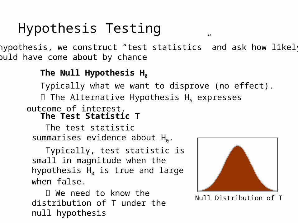
Hypothesis Testing

The Null Hypothesis H0

Typically what we want to disprove (no effect). The Alternative Hypothesis HA expresses outcome of interest.

To test an hypothesis, we construct “test statistics” and ask how likely that our statistic could have come about by chance

The Test Statistic T

The test statistic summarises evidence about H0.

Typically, test statistic is small in magnitude when the hypothesis H0 is true and large when false.

We need to know the distribution of T under the null hypothesis

Null Distribution of T

Test Statistics

An example (One-sample t-test):

SE = /N

Can estimate SE using sample st dev, s:

SE estimated = s/ N

t = sample mean – population mean/SE

t gives information about differences expected under H0 (due to sampling error).

Sampling distribution of mean xfor large N

Population

/N

How likely is it that our statistic could

have come from the null distribution?

Hypothesis Testing

P-value:

A p-value summarises evidence against H0.

This is the chance of observing value more extreme than t under the null hypothesis.

Observation of test statistic t, a realisation of T Null Distribution of T

)|( 0HtTp

Significance level α: Acceptable false positive rate α. threshold uα

Threshold uα controls the false positive rate

t

P-val

Null Distribution of T

u

The conclusion about the hypothesis: We reject the null hypothesis in favour of the

alternative hypothesis if t > uα

)|( 0HuTp

In GLM we test hypotheses about

- is a point estimator of the population

value- has a sampling distribution- has a standard error

-> We can calculate a t-statistic based on a null hypothesis about population

e.g. H0: = 0

Y = X + e

T-test on : a simple example

Q: activation during listening ?

cT = [ 1 0 ]

Null hypothesis: 01

)ˆ(

ˆ

T

T

cStd

ct

Passive word listening versus rest

SPMresults:Height threshold T = 3.2057 {p<0.001}

Design matrix

0.5 1 1.5 2 2.5

10

20

30

40

50

60

70

80

X

1

T =

contrast ofestimated

parameters

varianceestimate

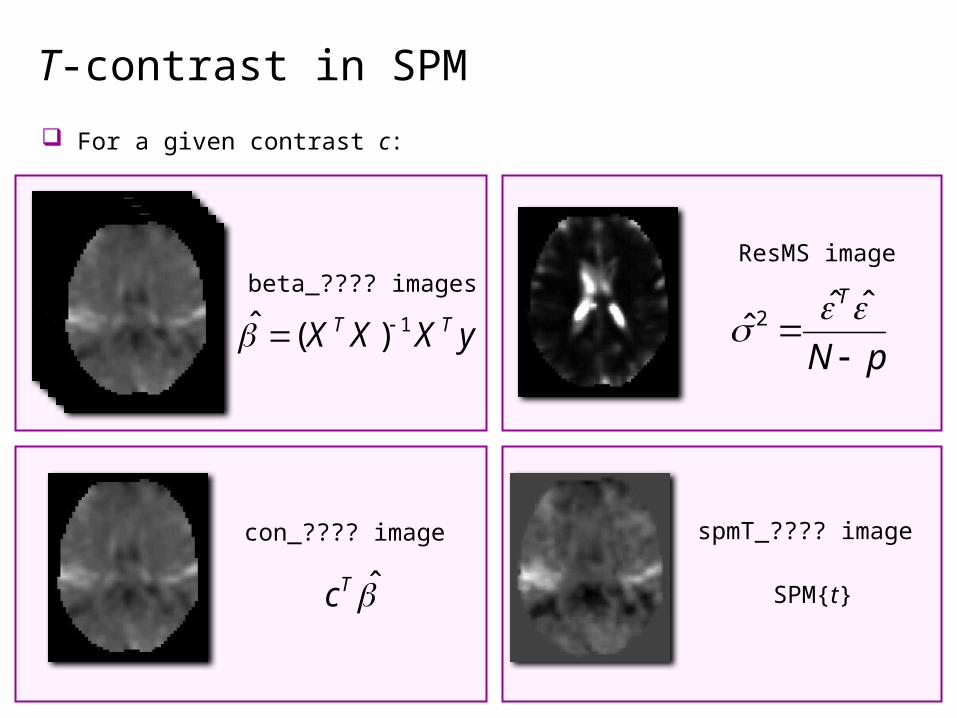
T-contrast in SPM

ResMS image

yXXX TT 1)(ˆ

con_???? image

Tc

pN

T

ˆˆ

ˆ 2

beta_???? images

spmT_???? image

SPM{t}

For a given contrast c:

How to do inference on t-maps?- T-map for whole brain may contain say

60000 voxels

- Each analysed separately would mean

60000 t-tests

- At = 0.05 this would be 3000 false positives (Type 1 Errors)

- Adjust threshold so that any values above threshold are unlikely to under the null hypothesis (height thresholding)

t > 0.5 t > 1.5 t > 2.5 t > 3.5 t > 4.5 t > 5.5 t > 6.5t > 0.5

A t-image!

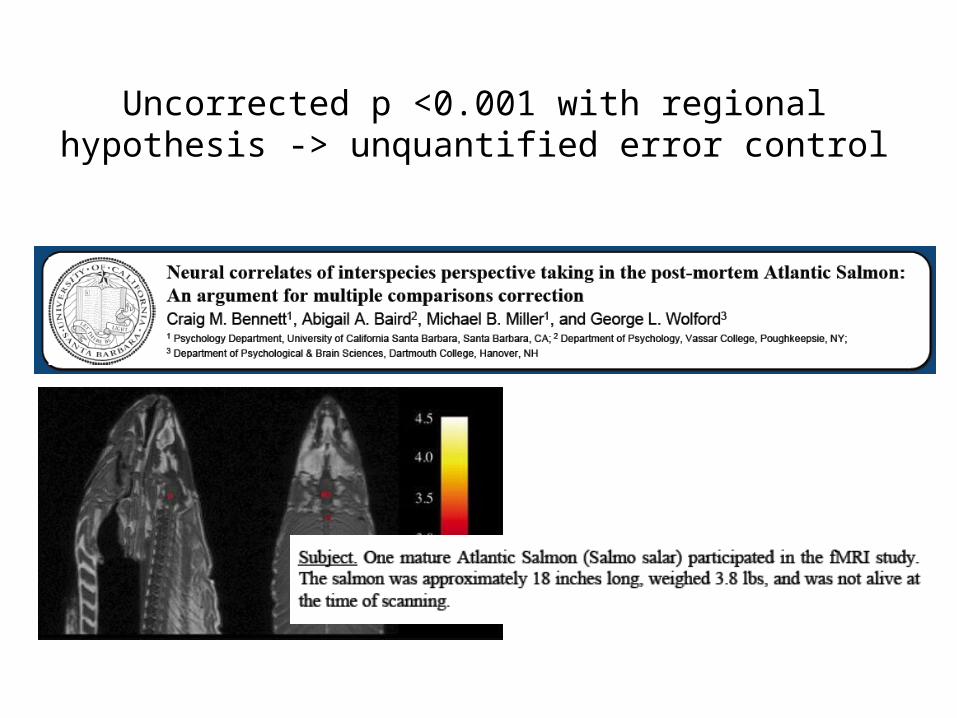
Uncorrected p <0.001 with regional hypothesis -> unquantified error control

Classical Approach to Multiple Comparison

Bonferrroni Correction:

A method of setting the significance threshold to control the Family-wise Error Rate (FWER)

FWER is probability that one or more values among a family of statistics will be greater than

For each test:

Probability greater than threshold: Probability less than threshold: 1-


Probability that all n tests are less than : (1- )n

Probability that one or more tests are greater than :

PFWE = 1 – (1- )n

Since is small, approximates to:

PFWE n .

= PFWE / n


= PFWE / n

Could in principle find a single-voxel probability threshold, , that would give the required FWER such that there would be PFWE probability of seeing any voxel above threshold in all of the n values...


= PFWE / n

e.g. 100,000 t stats, all with 40 d.f.

For PFWE of 0.05:

0.05/100000 = 0.0000005, corresponding t 5.77

=> a voxel statistic of >5.77 has only a 5% chance of arising anywhere in a volume of 100,000 t stats drawn from the null distribution

Why not Bonferroni?• Functional imaging data has a degree of spatial

correlation • Number of independent values < number of

voxels

Why?

• The way that the scanner collects and reconstructs the image

• Physiology• Spatial preprocessing (resampling, smoothing)

• Also could be seen as a categorical error: unique situation in which have a continuous statistic image, not a series of independent tests

Carlo Emilio Bonferroni was born in Bergamo on 28 January 1892 and died on 18 August 1960 in

Firenze (Florence). He studied in Torino

(Turin), held a post as assistant professor at the Turin Polytechnic,

and in 1923 took up the chair of financial mathematics at the

Economics Institute in Bari. In 1933 he

transferred to Firenze where he held his chair until his death.

Illustration of Spatial Correlation• Take an image slice, say 100 by 100 voxels

• Fill each voxel with an independent random sample from a normal distribution• Creates a Z-map (equivalent to t with v high d.f.)• How many numbers in the image are more positive than is likely by chance?

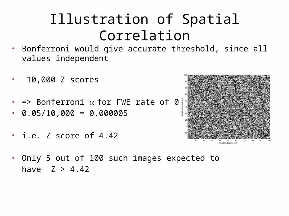
Illustration of Spatial Correlation• Bonferroni would give accurate threshold, since all values independent

• 10,000 Z scores

• => Bonferroni for FWE rate of 0.05• 0.05/10,000 = 0.000005

• i.e. Z score of 4.42

• Only 5 out of 100 such images expected to

have Z > 4.42

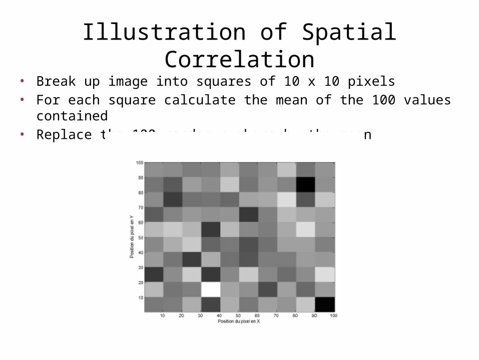
Illustration of Spatial Correlation• Break up image into squares of 10 x 10 pixels• For each square calculate the mean of the 100 values contained• Replace the 100 random numbers by the mean

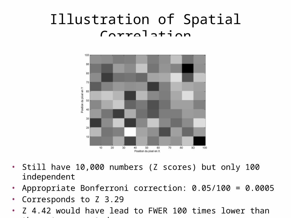
Illustration of Spatial Correlation

• Still have 10,000 numbers (Z scores) but only 100 independent• Appropriate Bonferroni correction: 0.05/100 = 0.0005• Corresponds to Z 3.29• Z 4.42 would have lead to FWER 100 times lower than the rate we

wanted

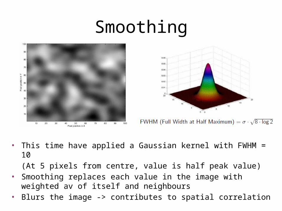
• This time have applied a Gaussian kernel with FWHM = 10

(At 5 pixels from centre, value is half peak value)• Smoothing replaces each value in the image with weighted av of itself and

neighbours• Blurs the image -> contributes to spatial correlation

Smoothing

Smoothing kernel

FWHM(Full Width at Half Maximum)

• Increases signal : noise ratio (matched filter theorem)

• Allow averaging across subjects (smooths over residual anatomical diffs)

• Lattice approximation to continuous underlying random field -> topological inference

• FWHM must be substantially greater than voxel size

Why Smooth?

Part 2: Random Field Theory

Outline

• Where are we up to?• Hypothesis testing• Multiple Comparisons vs Topological Inference• Smoothing• Random Field Theory• Alternatives• Conclusion• Practical example

Random Field Theory

The key difference between statistical parametric mapping (SPM) and conventional statistics lies in the thing one is making an inference about.

In conventional statistics, this is usual a scalar quantity (i.e. a model parameter) that generates measurements, such as reaction times.

[…]In contrast, in SPM one makes inferences about the topological features of a statistical process that is a function of space or time. (Friston, 2007)

Random field theory regards data as realizations of a continuous process in one or more dimensions.

This contrasts with classical approaches like the Bonferroni correction, which consider images as collections of discrete samples with no

continuity properties. (Kilner & Friston, 2010)

Why Random Field Theory?

• Therefore: Bonferroni-correction not only unsuitable because of spatial correlation– But also because of controlling something

completely different from what we need– Suitable for different, independent tests, not

continuous image– Couldn’t we think of each voxel as independent

sample?


• No• Imagine 100,000 voxels, α = 5%

– expect 5,000 voxels to be false positives• Now: halving the size of each voxel

– 200,000 voxels, α = 5%– Expect 40,000 voxels to be false positives

• Double the number of voxels (e.g. by increasing resolution) leads to an increase in false positives by factor of eight!– Without changing the actual data


• In RFT we are NOT controlling for the expected number of false positive voxels– false positive rate expressed as connected sets of

voxels above some threshold• RFT controls the expected number of false

positive regions, not voxels (like in Bonferroni)– Number of voxels irrelevant because being more

or less arbitrary – Region is topological feature, voxel is not


• So standard correction for multiple comparisons doesn’t work..– Solution: treating SPMs as discretisation of

underlying continuous fields• With topological features such as amplitude, cluster

size, number of clusters, etc.• Apply topological inference to detect activations in

SPMs

Topological Inference

• Topological inference can be about– Peak height– Cluster extent– Number of clusters

space

inte

nsity

t

tclus

Random Field Theory: Resels

• Solution: discounting voxel size by expressing search volume in resels– “resolution elements” – Depending on smoothness of data– “restoring” independence of data

• Resel defined as volume with same size as FWHM– Ri = FWHMx x FWHMy x FWHMz

Random Field Theory: Resels• Example before:

• Reducing 100 x 100 = 10,000 pixels by FWHM of 10 pixels

• Therefore: FWHMx x FWHMy = 10 x 10 = 100– Resel as a block of 100 pixels– 100 resels for image with 10,000 pixels

Random Field Theory: Euler Characteristic

• Euler Characteristic (EC) to determine height threshold for smooth statistical map given a certain FWE-rate– Property of an image after being thresholded– In our case: expected number of blobs in image

after thresholding


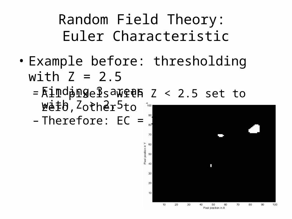
• Example before: thresholding with Z = 2.5– All pixels with Z < 2.5 set to zero, other to 1– Finding 3 areas with Z > 2.5– Therefore: EC = 3


• Increasing to Z = 2.75– All pixels with Z < 2.75 set to zero, other to 1– Finding 1 area with Z > 2.75– Therefore: EC = 1


• Expected EC (E[EC]) corresponds to finding an above threshold blob in statistic image– Therefore: PFWE ≈ E[EC]

• At high thresholds EC is either 0 or 1

EC a bit more complex than simply number of blobs (Worsleyet al., 1994)… Good approximation

FWE


• Why is E[EC] only a good approximation to PFWE if threshold sufficiently high?– Because EC basically is N(blobs) – N(holes)


• But if threshold is sufficiently high, then..– E[EC] = N(blobs)


• Knowing the number of resels R, we can calculate E[EC] as:PFWE ≈ E[EC] =

– : search volume– : smoothness

• Remember: – FWHM = 10 pixels– size of one resel: FWHMx x FWHMy = 10 x 10 = 100 pixels

– V = 10,000 pixels– R = 10,000/100 = 100

(for 3D)


• Knowing the number of resels R, we can calculate E[EC] as:PFWE ≈ E[EC] =

• Therefore: – if increases (increasing smoothness), R decreases

• PFWE decreases (less severe correction)

– If V increases (increasing volume), R increases• PFWE increases (stronger correction)

• Therefore: greater smoothness and smaller volume means less severe multiple testing problem– And less stringent correction

(for 3D)

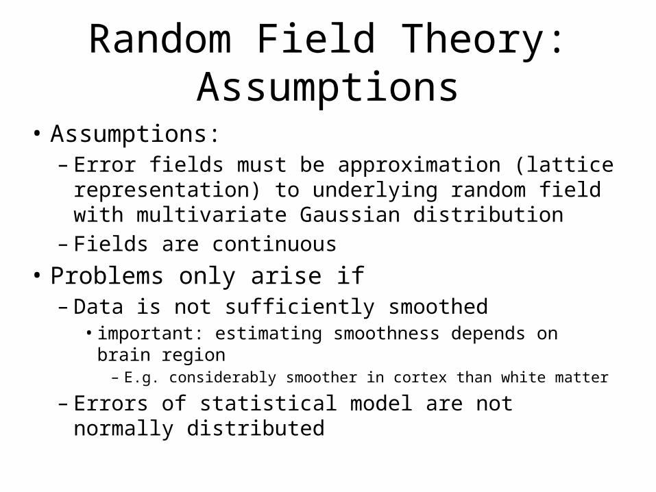
Random Field Theory: Assumptions

• Assumptions:– Error fields must be approximation (lattice

representation) to underlying random field with multivariate Gaussian distribution

lattice representation

Random Field Theory: Assumptions

• Assumptions:– Error fields must be approximation (lattice

representation) to underlying random field with multivariate Gaussian distribution

– Fields are continuous• Problems only arise if

– Data is not sufficiently smoothed• important: estimating smoothness depends on brain region

– E.g. considerably smoother in cortex than white matter

– Errors of statistical model are not normally distributed

Alternatives to FWE: False Discovery Rate

• Completely different (not in FWE-framework)– Instead of controlling probability of ever reporting false

positive (e.g. α = 5%), controlling false discovery rate (FDR)

– Expected proportion of false positives amongst those voxels declared positive (discoveries)

• Calculate uncorrected P-values for voxels and rank order them– P1 P2 … PN

• Find largest value k, so that Pk < αk/N


• But: different interpretation:– False positives will be detected– Simply controlling that they make up no more

than α of our discoveries– FWE controls probability of ever reporting false

positives• Therefore: better greater sensitivity, but lower

specificity (greater false positive risk)– No spatial specificity


Alternatives to FWE

• Permutation– Gaussian data simulated and smoothed based on real

data (cf. Monte Carlo methods)– Create surrogate statistic images under null hypothesis– Compare to real data set

• Nonparametric tests– Similar to permutation, but use empirical data set and

permute subjects (e.g. in group analysis)– E.g. construct distribution of maximum statistic with

repeated permutation within data

Conclusion

• Neuroimaging data needs to be controlled for multiple comparisons– Standard approaches don’t apply

• Inferences can be made voxel-wise, cluster-wise and set-wise• Inference is made about topological features

– Peak height, spatial extent, number of clusters• Random Field Theory provides valuable solution to multiple

comparison problem– Treating SPMs as discretization of continuous (random) field

• Alternatives to FWE (RFT) are False Discovery Rate (FDR) and permutation tests

Part 3: SPM Example

18/11/2009 RFT for dummies - Part II 5353

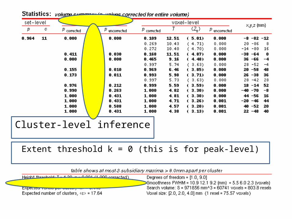
Results in SPMMaximum Intensity

Projection on Glass Brain


60,741 Voxels803.8 Resels

This screen shows all clusters above a chosen significance, as well as separate maxima within a cluster


Height threshold T= 4.30

Peak-level inferenceThis example uses uncorrected

p (!)


MNI Coords of each Max

Peak-level inference


Chance of finding peak above this threshold, corrected for search volume

Peak-level inference


Extent threshold k = 0 (this is for peak-level)

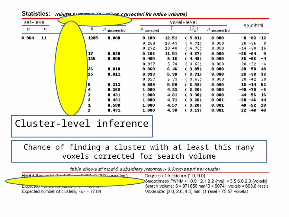
Cluster-level inference


Chance of finding a cluster with at least this many voxels corrected for search volume

Cluster-level inference


Chance of finding this or greater number of clusters in the search volume

Set-level inference

Thank you for listening

… and special thanks to Guillaume Flandin!

References• Kilner, J., & Friston, K. J. (2010). Topological inference for EEG and MEG

data. Annals of Applied Statistics, 4, 1272-1290.• Nichols, T., & Hayasaka, S. (2003). Controlling the familywise error rate in

functional neuroimaging: a comparative review. Statistical Methods in Medical Research, 12, 419-446.

• Nichols, T. (2012). Multiple testing corrections, nonparametric methods and random field theory. Neuroimage, 62, 811-815.

• Chapters 17-21 in Statistical Parametric Mapping by Karl Friston et al.• Poldrack, R. A., Mumford, J. A., & Nichols, T. (2011). Handbook of

Functional MRI Data Analysis. New York, NY: Cambridge University Press.• Huettel, S. A., Song, A. W., & McCarthy, G. (2009). Functional Magnetic

Resonance Imaging, 2nd edition. Sunderland, MA: Sinauer.• http://www.fil.ion.ucl.ac.uk/spm/doc/biblio/Keyword/RFT.html

Documents

Random Field Theory Giles Story Philipp Schwartenbeck Methods for dummies 2012/13 With thanks to Guillaume Flandin