Random Dry Markets and Statistical ArbitrageBounds for European Derivatives

João Amaro de Matos1

Faculdade de EconomiaUniversidade Nova de LisboaCampus de Campolide1099-032 Lisboa, Portugal

Ana LacerdaDepartment of StatisticsColumbia University

1255 Amsterdam AvenueNew York, NY 100027, USA

October 27, 2005

1Corresponding author. Email: amatos@fe.unl.pt.

Abstract

We derive statistical arbitrage bounds for the buying and selling price ofEuropean derivatives under incomplete markets. In this paper, incomplete-ness is generated due to the fact that the market is dry, i.e., the underlyingasset cannot be transacted at certain points in time. In particular, we re-fine the notion of statistical arbitrage in order to extend the procedure forthe case where dryness is random, i.e., at each point in time the asset canbe transacted with a given probability. We analytically characterize severalproperties of the statistical arbitrage-free interval, show that it is narrowerthan the super-replication interval and dominates somehow alternative in-tervals provided in the literarture. Moreover, we show that, for sufficientlyincomplete markets, the statistical arbitrage interval contains the reserva-tion price of the derivative.

1 Introduction

In complete markets and under the absence of arbitrage opportunities, the

value of a call option must be the same as the cheapest portfolio that repli-

cates exactly the value of the derivative at any given point in time. However,

in the presence of some market imperfections markets may become incom-

plete and it is not possible to exactly replicate the value of the call option

at all times anymore. Nevertheless, it is possible to derive an arbitrage-free

range of variation for the value of the derivative. This interval depends on

two different factors. First, on the nature of market incompleteness; Second,

on the notion of arbitrage opportunities.

In what follows we consider that market incompleteness is generated

by the fact that agents cannot trade the underlying asset on which the

derivative is written whenever they please. In fact, and as opposed to the

traditional asset pricing assumptions, markets are very rarely liquid and im-

mediacy is not always available. As Longstaff (1995, 2001, 2004) recalls,

the relevance of this fact is pervasive through many financial markets. The

markets for many assets such as human capital, business partnerships, pen-

sion plans, saving bonds, annuities, trusts, inheritances and residential real

estate, among others, are generally very illiquid and long periods of time

(months, sometimes years) may be required to sell an asset. This point

becomes extremely relevant for the case of option pricing when we consider

that it is an increasingly common phenomenon even in well-established se-

curities markets, as illustrated by the 1998 Russian default crisis, leading

many traders to be trapped in risky positions they could not unwind.

To address the impact of this issue on derivatives’ pricing, we consider

a discrete-time setting such that transactions are not possible within a sub-

set of points in time. Although clearly very stylized, the advantage of this

setting is that it incorporates in a very simple way the notion of market illiq-

uidity as the absence of immediacy. In this framework, illiquidity changes

what is otherwise a complete market into a dynamically incomplete market.

This was also the approach in Amaro de Matos and Antão (2001) when

characterizing the specific superreplication bounds for options in such mar-

1

kets and its implications. We further extend this setting by randomizing

the points in time where there are no transactions on the underlying asset,

reflecting a more realistic ex-ante uncertainty about the market illiquidity.

As stressed above, there is not a unique price for a derivative under mar-

ket incompleteness. However, for any given option, portfolios can be found

that have the same payoff as the option in some states of nature, and higher

payoffs in the other states. Such portfolios are said to be superreplicating.

Holding such a portfolio should be worth more than the option itself and

therefore, the value of the cheapest of such portfolios should be seen as an

upper bound on the selling value of the option. Similarly, a lower bound

for the buying price can be constructed. The nature of the superreplicating

bounds is well characterized in the context of incomplete markets in the

papers by El Karoui and Quenez (1991,1995), Edirisinghe, Naik and Uppal

(1993) and Karatzas and Kou (1996). The superreplicating bounds establish

the limits of the interval for arbitrage-free value of the option. If the price is

outside this range, then a positive profit is attainable with probability one.

In other words, an arbitrage opportunity exists if the option is sold above

the upper bound or bought below the lower bound.

Most of the times, however, these superreplicating bounds are trivial, in

the sense that they are too broad, not allowing a useful characterization of

equilibrium prices’ vicinity. As an alternative, Bernardo and Ledoit (2000)

propose a utility-based approach, restricting the no-arbitrage condition to

rule out investment opportunities offering high gain-loss ratios, where gain

(loss) is the expected positive (negative) part of excess payoff. In this way,

narrower bounds are obtained. Analogously, Cochrane and Saá-Requejo

(2000) also restrict the no-arbitrage condition by not allowing transactions of

“good deals”, i.e. assets with very high Sharpe ratio. Following Hansen and

Jagannathan (1991), they show that this restriction imposes an upper bound

on the pricing kernel volatility and leads to narrower pricing implications

when markets are incomplete.

Given a set of pricing kernels compatible with the absence of arbitrage

opportunities, Cochrane and Sáa-Requejo exclude pricing kernels implying

2

very high Sharpe ratios, whereas Bernardo and Ledoit exclude pricing ker-

nels implying very high gain-loss ratios, for a benchmark utility. Notice

that, for a different utility, Bernardo and Ledoit would exclude a different

subset of pricing kernels, for the same levels of acceptable gain-loss ratios.

In order to avoid ad-hoc thresholds in either Sharpe or gain-loss ratios,

or to make some parametric assumptions about a benchmark pricing kernel,

as in Bernardo and Ledoit (2000), the work of Bondarenko (2003) introduces

the notion of statistical arbitrage opportunity, by imposing a weak assump-

tion on a functional form of admissible pricing kernels, yielding narrower

pricing implications as compared to the superreplication bounds. A statisti-

cal arbitrage opportunity is characterized as a zero-cost trading strategy for

which (i) the expected payoff is positive, and (ii) the conditional expected

payoff in each final state of the economy is nonnegative. Unlike a pure arbi-

trage opportunity, a statistical arbitrage opportunity may allow for negative

payoffs, provided that the average payoff in each final state is nonnegative.

In particular, ruling out statistical arbitrage opportunities imposes a novel

martingale-type restriction on the dynamics of securities prices. The impor-

tant properties of the restriction are that it is model-free, in the sense that it

requires no parametric assumptions about the true equilibrium model, and

continues to hold when investors’ beliefs are mistaken.

In this paper we extend the notion of statistical arbitrage opportunity

to the case where the underlying asset cannot be transacted at a random

number of points in time and compare the statistical arbitrage-free bounds

with the superreplication bounds. We show that the statistical arbitrage-

free interval is narrower than the pure arbitrage bounds, and show also that,

for sufficiently incomplete markets, the statistical arbitrage interval contains

the reservation price of the derivative. We also provide examples that allow

comparison with the results of Cochrane and Saá-Requejo (2000) and discuss

the comparison with Bernardo and Ledoit (2000).

This paper is organized as follows. In section 2, the model is presented

and the pure arbitrage results are derived. In section 3 the notion of sta-

tistical arbitrage in the spirit of Bondarenko (2003) is defined. In section

3

4, the main results are presented. In Section 5 we first characterize the

reservation prices and then show that, in a sufficiently dry market, they are

contained in the statistical arbitrage interval. In Section 6 we illustrate how

the statistical arbitrage-free interval somehow dominates alternative inter-

vals provided in the literature. In section 7 some numerical examples are

presented in order to illustrate some important properties of the bounds. In

the last section several conclusions are presented.

2 The Model

Consider a discrete-time economy with T periods, with a risky asset and

a riskless asset. At each point in time the price of the risky asset can be

multiplied either by U or by D to get the price of the next point in time.

Equilibrium requires that U > R > D, whereR denotes one plus the risk-free

interest rate. At time t = 0 and t = T transactions are certainly possible.

However, at t = 1, ..., T − 1 there is uncertainty about the possibility oftransaction of the risky asset. Transactions will occur with probability p at

each of these points in time. A European Call option with exercise price K

and maturity T is considered.

Consider the Binomial tree process followed by the price of the risky

asset. Let the set of nodes at date t be denoted by It, and let each of the

t + 1 elements of It be denoted by it = 1, . . . , t + 1. For any t0 < t, let Iitt0

denote the set of all the nodes at time t0that are predecessors of a given

node it. A path on the event tree is a set of nodes w = ∪t∈0,1,...,Tit suchthat each element in the union satisfies it−1 ∈ Iitt−1. Let Ω denote the set ofall paths on the event tree.

At each node it, there is a number ∆itt representing the number of shares

bought (or sold, if negative), and a number Bitt denoting the amount invested

(or borrowed, if negative) in the risk-free asset. Hence, at date t there are

t+1 different values of∆itt , composing a vector∆t ≡ (∆1t , . . . ,∆t+1t ) ∈ Rt+1.Similarly, we construct the vector Bt ≡ (B1t , . . . , Bt+1t ) ∈ Rt+1.

Definition 1 A trading strategy is a portfolio process θt = (∆t, Bt) , com-

4

posed of ∆t units of the risky asset and an amount Bt invested in the riskless

asset, such that the portfolio’s cost is ∆tSt +Bt for t = 0, 1, . . . T − 1.

In order to find the upper (lower) bound of the arbitrage-free range of

variation for the value of the call option we consider a financial institution

that wishes to be fully hedged when selling (buying) that option. The objec-

tive of the institution is to minimize (maximize) the cost of replicating the

exercise value of the option at maturity. The value determined under such

optimization procedure avoids what is known as arbitrage opportunities,

reflecting the possibility of certain profits at zero cost.

This section is organized as follows. We first characterize the upper

bound, and then the lower bound for the interval of no-arbitrage admissi-

ble prices. For each bound, we first deal with the complete market case,

and then with the fully incomplete market case, finally introducing random

incompleteness.

2.1 The upper bound in the case p = 0 and p = 1.

First, we present the well-known case where p = 1. The usual definition of

an arbitrage opportunity in our economy is as follows.

Definition 2 (Pure Arbitrage in the case p = 1) In this economy, an

arbitrage opportunity is a zero cost trading strategy θt such that

1. the value of the portfolio is positive at any final node, i.e.,

∆iT−1T−1S

iTT +RB

iT−1T−1 ≥ 0,

for any iT−1 ∈ IiTT−1 and all iT ∈ IT ; and2. the portfolio is self-financing, i.e.,

∆it−1t−1 S

itt +RB

it−1t−1 ≥ ∆

itt S

itt +B

itt ,

for any it−1 ∈ Iitt−1, all it ∈ It and all t ∈ 0, ..., T − 1 .

The upper bound for the value of the European option is the maximum

value for which the derivative can be transacted, without allowing for ar-

bitrage opportunities. This is the value of the cheapest portfolio that the

5

seller of the derivative can buy in order to completely hedge his position

against the exercise at maturity, without the need of additional financing at

any rebalancing dates. Hence, for p = 1, the upper bound is C1u, given by

C1u = min∆t,Btt=0,....,T−1

∆0S0 +B0

subject to

∆iT−1T−1S

iTT +RB

iT−1T−1 ≥

³SiTT −K

´+,

with iT−1 ∈ IiTT−1 and all iT ∈ IT , and the self-financing constraints

∆it−1t−1 S

itt +RB

it−1t−1 ≥ ∆

itt S

itt +B

itt ,

for all it−1 ∈ Iitt−1, all it ∈ It and all t ∈ 0, ..., T − 1 , where the constraintsreflect the absence of arbitrage opportunities. This problem leads to the

familiar result

C1u =1

RT

TXj=0

µT

j

¶µR−DU −D

¶j µU −RU −D

¶T−j ¡U jDT−jS0 −K

¢+.

Consider now the case where p = 0. In this case, the notion of a trading

strategy satisfying the self-financing constraint is innocuous, since the port-

folio θt cannot be rebalanced during the life of the option. Under the absence

of arbitrage opportunities, the upper bound for the value is C0u satisfying

C0u = min∆0,B0

∆0S0 +B0

subject to

∆0SiTT +RT∆0 ≥

³SiTT −K

´+,

for all iT ∈ IT . In this case, the bound is given by1

C0u =1

RT

∙µRT −DTUT −DT

¶¡UTS0 −K

¢++

µUT −RTUT −DT

¶¡DTS0 −K

¢+¸.

1See Amaro de Matos and Antão (2001).

6

2.2 The lower bound in the case p = 0 and p = 1.

The lower bound for the value of an American derivative is the minimum

value for which the derivative can be transacted without allowing for arbi-

trage opportunities. This is the value of the most expensive portfolio that

the buyer of the option can sell in order to be fully hedged, and without the

need of additional financing at rebalancing dates.

For p = 1, the lower bound for the value of the derivative under the

absence of arbitrage opportunities is thus C1l , given by

C1l = max∆t,Btt=0,....,T−1

∆0S0 +B0

subject to

∆iT−1T−1S

iTT +RB

iT−1T−1 ≤

³SiTT −K

´+with iT−1 ∈ IiTT−1 and all iT ∈ IT , and the self-financing constraints

∆it−1t−1 S

itt +RB

it−1t−1 ≤ ∆itt Sitt +Bitt ,

for all it−1 ∈ Iitt−1, all it ∈ It and all t ∈ 0, ..., T − 1 , where the constraintsreflect the absence of arbitrage opportunities This problem leads to the

familiar result

C1l =1

RT

TXj=0

µT

j

¶µR−DU −D

¶j µU −RU −D

¶T−j ¡U jDT−jS0 −K

¢+, (1)

that coincides with the solution obtained for C1u.

In the case where p = 0, the lower bound for the value of the derivative

is C0l , satisfying

C0l = max∆0,B0

∆0S0 +B0

subject to

∆0ST +RTB0 ≤ (ST −K)+ .

7

It follows that this bound is given by2

C0l =1

RT

ÃRT − UT−(i+1)Di+1

UT−iDi − UT−(i+1)Di+1

!¡UT−iDiS0 −K

¢+(2)

+1

RT

µUT−iDi −RT

UT−iDi − UT−(i+1)Di+1

¶¡UT−i−1Di+1S0 −K

¢+.

where i is defined as the unique integer satisfying Un−(i+1)Di+1 < Rn <

Un−iDi, and 0 ≤ i ≤ n− 1.

2.3 The Bounds on Probabilistic Markets

In the aforementioned cases we considered the cases where either p = 0 or

p = 1. However, if p is not equal to neither 0 nor 1, the formulation has to

be adjusted. If the risky asset can be transacted with a given probability

p ∈ (0, 1), then the usual definition of arbitrage opportunity reads as follows.

Definition 3 (Pure Arbitrage for p ∈ (0, 1)) In this economy, an arbi-trage opportunity is a zero cost trading strategy such that

1. the value of the portfolio is positive at any final node, i.e.,

∆itt SiTT +RT−tBitt ≥ 0,

it ∈ IiTt and all iT ∈ IT ; and the self-financing constraints2. the portfolio is self-financing, i.e.,

∆it−jt−j S

itt +R

jBit−jt−j ≥ ∆

itt S

itt +B

itt ,

for all it−j ∈ Iitt−j , all it ∈ It and all t ∈ 0, ..., T − 1 .

The upper bound Cpu is the solution of the following problem:

Cpu = min∆t,Btt=0,...,T−1

∆0S0 +B0

where ∆t, Bt ∈ Rt+1, t = 0, ..., T − 1, subject to the superreplicating condi-tions

∆itt SiTT +RT−tBitt ≥

³SiTT −K

´+,

2See Amaro de Matos and Antão (2001).

8

with it ∈ IiTt and all iT ∈ IT , and the self-financing constraints

∆it−jt−j S

itt +R

jBit−jt−j ≥ ∆

itt S

itt +B

itt

for all it−j ∈ Iitt−j , all it ∈ It and all t ∈ 0, ..., T − 1 .On the other hand, the lower bound Cpl solves the following problem:

Cpl = max∆t,Btt=0,...,T−1

∆0S0 +B0

where ∆t, Bt ∈ Rt+1, t = 0, ..., T − 1, subject to the conditions

∆itt SiTT +RT−tBitt ≤

³SiTT −K

´+,

with it ∈ IiTt and all iT ∈ IT , and the self-financing constraints

∆it−jt−j S

itt +R

jBit−jt−j ≤ ∆

itt S

itt +B

itt

for all it−j ∈ Iitt−j , all it ∈ It and all t ∈ 0, ..., T − 1 .Notice that the constraints in the above optimization problems are im-

plied by the absence of arbitrage opportunities and do not depend on the

probability p.3 Therefore, neither Cpu nor Cpl will depend on p. We are now

in conditions to relate these values to C0u and C0l as follows.

Theorem 4 For p ∈ (0, 1) the upper and lower bound for the prices above donot depend on p. The optimization problems above lead to the same solutions

as when p = 0.

Proof. Consider first the case of the upper bound. The constraints

characterizing Cpu include all the constraints characterizing C0u. Thus, Cpu ≥

C0u. Now, let ∆00 and B

00 denote the optimal values invested, at time t = 0,

when p = 0. The trading strategy ∆pt = ∆00 and Bpt = RtB00 , for all

t = 1, ..., T − 1, is an admissible strategy for any given p, hence Cpu = C0u.The case of the lower bound is analogous.

3This happens since, in order to have an arbitrage opportunity, we must ensure that,whether market exists or not at each time t ∈ 1, ..., T − 1 , the agent will never losewealth. Therefore, the optimization problem cannot depend on p.

9

The intuition for this result is straightforward. The upper (lower) bound

of the call option remains the same as when p = 0, because with probabil-

ity 1 − p it would not be possible to transact the stock at each point intime. In order to be fully hedged, as required by the absence of arbitrage

opportunities, the worse scenario will be restrictive in spite of its possibly

low probability. The fact that no intermediate transactions may occur dom-

inates all other possibilities.

The above result is strongly driven by the definition of arbitrage oppor-

tunities. Nevertheless, if this notion is relaxed in an economic sensible way,

a narrower arbitrage-free range of variation for the value of the call option

may be obtained, possibly depending now on p. This is the subject of the

rest of the paper.

3 Statistical Arbitrage Opportunity

Consider the economy described in the previous section. Let Tp = 1, ..., T − 1denote the set of points in time. At each of these points there is market with

probability p, and there is no market with probability 1− p. The existence(or not) of the market at time t corresponds to the realization of a random

variable yt that assumes the value 0 (when there is no market) and 1 (when

there is market). This random variable is defined for all t ∈ Tp and it isassumed to be independent of the ordinary source of uncertainty that gen-

erates the price process. We can therefore talk about a market existence

process. In order to construct one such process, let us start with the state

space. Let #(Tp) denote the number of points in Tp. At each of these points,market may either exist or not exist, leading to 2#(Tp) possible states of

nature. We then have the collection of possible states of nature denoted by

Ω = vii=1,...,2#(Tp) , each vi corresponding to a distinct state. Moreover,let F = F1, . . . , FT−1, where Ft is the σ-algebra generated by the randomvariable yt. Let py be the probability associated with the random variable

yt. For all t ∈ Tp, we have py (yt = 1) = p and py (yt = 0) = 1− p.

10

3.1 The expected value of a portfolio

We now construct a random variable that allows to construct the expected

future value of a portfolio in this setting. For t < t0, let xt,t0 be a random

variable identifying the last time that transactions take place before date t0,

given that we are at time t, and transactions are currently possible. Let Ωt

be the subset of Ω such that Ωt =nvi ∈ Ω : yt (vi) = 1

o. Then,

xt,t0 : Ωt →©t, . . . , t0 − 1

ªLet pxt,t0 be the probability associated with xt,t0 . Then,

pxt,t0¡xt,t0 = t

¢= (1− p)t0−t−1 .

Moreover, for a given s ∈ (t, t0) ,

pxt,t0¡xt,t0 = s

¢= p (1− p)t0−s−1 .

Also note thatXt0−1

s=tpxt,t0

¡xt,t0 = s

¢= (1− p)t0−t−1 +

Xt0−1

s=tp (1− p)t0−s−1 = 1,

as it should.

Consider a given trading strategy (∆t, Bt)t=0,... ,T , where (∆t, Bt) ≡(∆itt , B

itt )it∈It is a (t + 1)−dimensional vector. Consider a given path w

and (is)s∈t,... ,T ⊂ w. Suppose that the agent is at a given node it, whererebalancing is possible. As there is uncertainty about the existence of mar-

ket at the future points in time, there is also uncertainty about the portfolio

that the agent will be holding at a future node it0 . In fact, the portfolio at

it0 may be any of³∆itt , B

itt

´,³∆it+1t+1 , B

it+1t+1

´, . . . , or

³∆it0−1t0−1 , B

it0−1t0−1

´, where

(is)s∈t,... ,t0−1 ⊂ w.Clearly, the expected value of a given trading strategy at node it0 , given

that we are at node it, is

Epxt,t0it

h∆ixx S

it0 +R

t0−xBixx

i=X

s=t,... ,t0−1pxt,t0

¡xt,t0 = s

¢ h∆iss S

it0 +R

t0−sBiss

i,

where we use x to short notation for xt,t0 .

11

3.2 Statistical versus pure arbitrage

A pure arbitrage opportunity is a zero-cost portfolio at time t, such that the

value of each possible portfolio at node iT is positive, i.e.,

∆it+jt+j S

iTT +RT−t−jB

it+jt+j ≥ 0

for all it+j such that it is a predecessor, j = 0, 1, . . . , T − t− 1 and

Epxt,Tit

h∆ixx S

iTT +RT−xBixx

i> 0,

together with the self-financing constraints

∆itt Sit+jt+j +R

j−tBitt ≥ ∆it+jt+j S

it+jt+j +B

it+jt+j ,

for all it+j such that it is a predecessor, and j = 1, . . . , T − t− 1.If statistical arbitrage is considered, however, an arbitrage opportunity

requires only that, at node iT , the expected value of the portfolio at T is

positive,

Epxt,Tit

h∆ixx S

iTT +RT−xBixx

i≥ 0,

together with weaker self-financing conditions. Let us regard these latter

conditions in some detail.

Suppose that we are at a given node it. If there is market at the next

point in time we then have, for sure, the portfolio³∆itt , B

itt

´at time t+ 1.

Hence, if node it+1 is reached, the self-financing condition is

∆itt Sit+1t+1 +RB

itt −

³∆it+1t+1 S

it+1t+1 +B

it+1t+1

´≥ 0

Consider now that t+2 is reached. At time t there is uncertainty about

the existence of the market at time t + 1. Hence, at time t + 2 we can ei-

ther have the portfolio³∆itt , B

itt

´or the portfolio

³∆it+1t+1 , B

it+1t+1

´. Under the

concept of statistical arbitrage, we want to ensure that, in expected value,

we are not going to lose at node it+2. Hence, the self-financing condition

becomesXs=t,t+1

pxt,t+2 (xt,t+2 = s)³∆iss S

it+2t+2 +R

t+2−sBiss

´≥³∆it+2t+2 S

t+2t+2 +B

it+2t+2

´

12

More generally, for any t at which transaction occurs and t < t0 < T, the

statistical self-financing condition becomes

Epxt,t0

it

h∆ixx S

it0t0 +R

t0−xBixx

i≥³∆it0t0 S

it0t0 +B

it0t0

´Definition 5 4 A statistical arbitrage opportunity is a zero-cost trading

strategy for which

1. At any node it, the expected value of the portfolio at any final node

is positive, i.e.,

Epxt,Tit

h∆ixxt,TS

iT +R

T−xBixxt,T

i≥ 0

for any it ∈ It and t ∈ 0, 1, . . . , T − 1; and2. The portfolio is statistically self-financing, i.e.,

Epxt,t0

it

h∆ixxt,t0S

it0 +R

t0−xBixxt,t0

i−³∆it0t0 S

it0t0 +B

it0t0

´≥ 0

for any it ∈ It, t0 > t, t ∈ 0, 1, . . . , T − 2 and t0 ∈ 1, . . . , T − 1 .

The two definitions of arbitrage are related in the following.

Theorem 6 If there are no statistical arbitrage opportunities, then there

are no pure arbitrage opportunities.

Proof. If there is a pure arbitrage opportunity then the inequalities

present in the definition of arbitrage opportunity, definition 3, are respected.

4This notion of Arbitrage Opportunity is in the spirit of Bondarenko (2003). In hisdefinition 2, a Statistical Arbitrage Opportunity (SAO) is defined as a zero-cost tradingstrategy with a payoff ZT = Z (FT ), such that

(i) E [ZT |F0] > 0, and(ii) E [ZT |F0; ξT ] ≥ 0, for all ξT ,

where ξt denotes the state of the Nature at time t, and Ft = (ξ1, . . . , ξt) is the marketinformation set, with F0 = φ. Also, the second expectation is taken at time t = 0 andis conditional to the terminal state ξT . However, notice that eliminating SAO’s at timet = 0 does not imply the absence of SAO’s at future times t ∈ [1, T − 1]. Hence, in orderto incorporate a dynamically consistent absence of SAO’s, we refine the definition of aSAO as a zero-cost trading strategy with a payoff ZT = Z (FT ), such that

(i) E [ZT |F0] > 0, and(ii) E [ZT |Ft; ξT ] ≥ 0, for all ξT and all t ∈ [0, T − 1] .

13

Hence, as these expressions are the terms under expectation in the definition

of Statistical Arbitrage opportunity, presented in definition 5, there is also

a statistical arbitrage opportunity.

The set of portfolios that represent a pure arbitrage opportunity is a

subset of the portfolios that represent a statistical arbitrage opportunity, i.e.,

there are portfolios that, in spite of not being a pure arbitrage opportunity,

represent a statistical arbitrage opportunity.

In order to have a statistical arbitrage opportunity it is not necessary

(although it is sufficient) that the value of the portfolio at the final date is

positive. It is only necessary that, for all t, the expected value of the portfolio

at the final date is positive.

Consider now the self-financing conditions under statistical arbitrage.

When rebalancing the portfolio it is not necessary (although it is sufficient)

that the value of the new portfolio is smaller than the value of the old one.

This happens because future rebalancing is uncertain, leading to uncertainty

about the portfolio that the agent will be holding in any future moment. In

order to avoid a statistical arbitrage opportunity it is only necessary that

the expected value of the portfolio at a given point in time is larger than the

value of the rebalancing portfolio.

Finally, notice that the concept of statistical arbitrage opportunity re-

duces to the usual concept of arbitrage opportunity in the limiting case

p = 0.

3.3 Augmented measures

For technical reasons, we now define an augmented probability space Q on

Ω. In order to do that, we define a semipath m from it to it0 , which is a set

of nodes m = ∪k∈t,... ,t0ik such that ik ∈ Iik+1k . Let Ω+it,it0 denote the set of

semipaths from it to it0 .

Definition 7 An augmented probability space in Ω is a set of probabilities

14

nq(iT ,T ),m(it,t)

osuch that it ∈ It, m ∈ Ω+it,iT , t = 0, . . . , T andX

iT

T−1Xt=0

Xit

Xm

q(iT ,T ),m(it,t)

= 1,

Definition 8 A modified martingale probability measure is an augmented

probability measure Q ∈ Q which satisfies

(i)

S0 =1

RT

XiT∈IT

qiTSiTT

where

qiT =T−1Xt=0

Xnit:it∈IiTt

oX

nm∈Ω+it,iT

o q(iT ,T ),m(it,t)SiTT ;

(ii)

SiT−1T−1 =

1

R

XniT :iT−1∈I

iTT−1

o π(iT ,T ),m(it,t)SiTT

with XniT :iT−1∈I

iTT−1

o π(iT ,T ),m(it,t)= 1

and

π(iT ,T ),m(it,t)

=1

Ξ

T−1Xt=0

pxt,T (xt,T = T − 1)X

nit:it∈I

iT−1t

oX

nm∈Ω+it,iT :iT−1∈m

o q(iT ,T ),m(it,t)

where

Ξ =T−1Xt=0

pxt,T (xt,T = T − 1)X

niT :iT−1∈I

iTT−1

oX

nit:it∈I

iT−1t

oX

nm∈Ω+it,iT :iT−1∈m

o q(iT ,T ),m(it,t);

(iii) there existsnα(it0 ,t

0),m(it,t)

o,for all it0 ∈ It0 , it ∈ It, m ∈ Ω+it,iT and

t0 > t for all t = 0, . . . , T − 1 such that, for all 0 < k < T,

Sikk =1

RT−k

XniT :ik∈I

iTk

o θ(iT ,T ),m(it,t)SiTT +

Xt0>k

1

Rt0−kε(it0 ,t

0),m(it,t)

Sit0t0 ,

15

where XniT :ik∈I

iTk

o θ(iT ,T ),m(it,t)+Xt0>k

ε(it0 ,t

0),m(it,t)

= 1

and

θ(iT ,T ),m(it,t)

=1

Θ

kXt=0

pxt,T (xt,T = k)Xn

it:it∈Iikt

o Xnm∈Ω+it,iT :ik∈m

o q(iT ,T ),m(it,t)

ε(it0 ,t

0),m(it,t)

=1

Θ

Xt<k

pxt,t0¡xt,t0 = k

¢Xnit:it∈I

ikt

o Xnm∈Ω+it,it :ik∈m

oα(it0 ,t0),m

(it,t)

with

Θ =X

niT :ik∈I

iTk

okXt=0

pxt,T (xt,T = k)Xn

it:it∈Iikt

o Xnm∈Ω+it,iT :ik∈m

o q(iT ,T ),m(it,t)+

Xt0>k

Xt<k

pxt,t0¡xt,t0 = k

¢Xnit:it∈I

ikt

o Xnm∈Ω+it,it :ik∈m

oα(it0 ,t0),m

(it,t).

We denote by QS. the set of modified martingale probability measure.

Such measures will help writing down the upper and lower bounds for the

value of European derivatives under the absence of statistical arbitrage op-

portunities.

4 Main Results

4.1 The upper bound

4.1.1 The Problem

The problem of determining the upper bound of the statistical arbitrage-free

range of variation for the value of a European call option, can be stated as

Cu = min∆t,Btt=0,...,T−1

∆0S0 +B0

where

∆t, Bt ∈ Rt+1, t = 0, ..., T − 1

16

subject to the conditions of a positive expected payoff

Epxt,Tit

£∆ixx S

iT +R

T−xBixx¤≥¡SiT −K

¢+,

for any it ∈ It and t ∈ 0, 1, . . . , T − 1 5, and self-financing conditions

Epxt,t0

it

h∆ixx S

it0 +R

t0−xBixx

i−³∆it0t0 S

it0t0 +B

it0t0

´≥ 0

for any it ∈ It, t0 > t, t ∈ 0, 1, . . . , T − 2 and t0 ∈ 1, . . . , T − 1 6.

Example 9 Illustration of the optimization problem with T = 3. The evo-

lution of the price underlying asset can be represented by the following tree

t=3t=2t=1t=0 t=3t=2t=1t=0

Figure 1: Evolution of the undelying asset’ price.

In what concerns the evolution of the price process there are eight differ-

ent states, i.e., Ω = wii=1,... ,8 . The problem that must be solved in order

to find the upper bound is the following.

Cu = min∆t,Btt=0,...,2

∆0S0 +B0

where

∆0, B0 = (∆0, B0)

∆1, B1 =©¡∆11, B

11

¢,¡∆21, B

21

¢ª∆2, B2 =

©¡∆12, B

12

¢,¡∆22, B

22

¢,¡∆32, B

32

¢ª5For each it there are 2(T−t) paths, and as a result, 2(T−t)(t+1) restrictions at time t.

The total number of restrictions isPT−1

t=0 2(T−t)(t+ 1).

6For each it there arePT−1

t0=t+1 2t0−t. Hence, for each t there are (t+ 1)

PT−1t0=t+1 2

t0−t.

Hence, there arePT−2

t=0 (t+ 1)PT−1

t0=t+1 2t0−t restrictions.

17

subject to the conditions of a positive expected payoffh∆i22 S

i33 +RB

i22

i≥³Si33 −K

´+for all i3 ∈ I3 and i2 ∈ I2 such that i2 ∈ Ii32 . (these are 6 constraints);

ph∆i22 S

i33 +RB

i22

i+ (1− p)

h∆i11 S

i33 +R

2Bi11

i≥³Si33 −K

´+for all i3 ∈ I3, i2 ∈ I2 and i1 ∈ I1 such that i2 ∈ Ii32 . and i1 ∈ I

i21 , i.e., i1, i2

and i3 belong to the same path (these are 8 constraints) and£p2 + p (1− p)

¤ h∆i22 S

i33 +RB

i22

i+ p (1− p)

h∆i11 S

i33 +R

2Bi11

i+

+(1− p)2h∆0S

i33 +R

3Bi22

i≥³Si33 −K

´+for all i3 ∈ I3, i2 ∈ I2 and i1 ∈ I1 such that i2 ∈ Ii32 . and i1 ∈ I

i21 , i.e., i1,

i2 and i3 belong to the same path (these are 8 constraints). Moreover, the

self-financing constraints must also be considered

∆0Si11 +RB0 ≥ ∆

i11 S

i11 +B

i11

for any i1 ∈ I1 (2 constraints),

(1− p)h∆0S

i22 +R

2Bi22

i+ p

h∆i11 S

i22 +RB

i11

i≥ ∆i22 S

i22 +B

i22

for any i2 ∈ I2 and i1 ∈ I1 such that i1 ∈ Ii21 , i.e., i1,and i2 belong to thesame path (these are 4 constraints) and, finally,

∆i11 Si22 +RB

i11 ≥ ∆

i22 S

i22 +B

i22

for any i2 ∈ I2 and i1 ∈ I1 such that i1 ∈ Ii21 , i.e., i1,and i2 belong to thesame path (these are 4 constraints).

4.1.2 Solution

Theorem 10 There exists a modified martingale probability measure, qiT ∈QS , such that the upper bound for arbitrage-free value of a European option

can be written as

Cu = maxqiT ∈QS

1

RT

XiT∈IT

qiThSiTT −K

i+. (3)

18

Proof. See proof in appendix A.1.

Remark 11 The values for qiT , in a model with two periods are explicitly

calculated in appendix A.3. In that case it can be shown that for a strictly

positive p, the q1, q2 and q3 are also strictly positive.

In what follows we characterize some relevant properties of Cu.

1. Cu ≤ C0u

Proof. Let ∆00 and B00denote the optimal values invested, at time

t = 0, in the stock and in the risk-free asset respectively, when p = 0.

The trading strategy ∆t = ∆P=00 and Bt = RtBp=00 , for t = 1, ..., T−1,

is an admissible strategy for any given p. As a result, the solution of

the problem for any p cannot be larger that the value of this portfolio

at t = 0 (which is C0u).

2. Cu ≥ C1u.

Proof. Consider the trading strategy¡∆∗t , B

∗t

¢t=0,... ,T−1 that solves

the maximization problem that characterizes the upper bound for a

p ∈ (0, 1) . This is an admissible strategy for the case p = 1, becauseit is self-financing, i.e.,

∆it−1t−1 S

itt +RB

it−1t−1 ≥ ∆

itt S

itt +B

itt ,

and superreplicates the payoff of the European derivative at maturity,

i.e.,

∆iT−1T−1S

iTT +RB

iT−1T−1 ≥

³SiTT −K

´+.

Hence, the solution of the problem for p = 1 cannot be higher than

the value of this portfolio at t = 0 (which is Cu).

3. limp→0Cu = C0u and limp→1Cu = C1u.

Proof. See Appendix A.4

An example for T=2 is also show in appendix A.4.

19

4. Cu is a decreasing function of p.

Proof. See Appendix A.4

5. For T = 2, we can prove that

Cu ≤ pC1u + (1− p)C0u

meaning that the probabilistic upper bound is a convex linear combi-

nation of the perfectly liquid upper bound and the perfectly illiquid

upper bound.

Proof. See appendix A.4.

4.2 The Lower Bound

The organization of this section is analogous to the section for the upper

bound.

4.2.1 The Problem

The problem of determining the lower bound of the statistical arbitrage-free

range of variation for the value of an European call option, can be stated as

Cl = max∆t,Btt=0,...,T−1

∆0S0 +B0

where

∆t, Bt ∈ Rt+1, t = 0, ..., T − 1

subject to the conditions of a positive expected payoff

Epxt,Tit

£∆ixx S

iT +R

T−xBixx¤≤¡SiT −K

¢+,

for any it ∈ It and t ∈ 0, 1, . . . , T − 1 7,and self-financing conditions

Epxt,t0

it

h∆ixx S

it0 +R

t0−xBixx

i−³∆it0t0 S

it0t0 +B

it0t0

´≤ 0

for any it ∈ It, t0 > t, t ∈ 0, 1, . . . , T − 2 and t0 ∈ 1, . . . , T − 1 8.7As in the upper bound case, for each it there are 2(T−t) paths, and as a result,

2(T−t)(t+1) restrictions at time t. The total number of restrictions isPT−1

t=0 2(T−t)(t+1).

8As in the upper bound case, for each it there arePT−1

t0=t+1 2t0−t. Hence, for each t

there are (t+ 1)PT−1

t0=t+1 2t0−t. Hence, there are

PT−2t=0 (t+ 1)

PT−1t0=t+1 2

t0−t restrictions.

20

4.2.2 Solution

Theorem 12 There exists an modified martingale probability measure, qiT ∈QS , such that the upper bound for arbitrage-free value of an European option

can be written as

Cl = minqiT ∈QS

1

RT

XiT∈IT

qiThSiTT −K

i+.

Proof. The proof is analogous to the upper bound.

Remark 13 The values for qiT , in a model with two periods are explicitly

calculated in appendix B.2. In that case it can be shown that for a strictly

positive p, the q1, q2 and q3 are also strictly positive.

In what follows we characterize some relevant properties of Cl.

1. Cl ≥ C0l .

2. Cl ≤ C1l .

3. limp→0Cl = C0l and limp→0Cl = C1l .

An example for T = 2 is shown in appendix B.3

4. Cl is a increasing function of p.

The proofs of these properties are analogous to those presented for the

upper bound.

5 Utility Functions and Reservation Prices

In this section we show that the price for which any agent is indifferent be-

tween transacting or not transacting the derivative, to be called the reser-

vation price of the derivative, is contained within the statistical arbitrage

bounds derived above.

Let ut (.) denote a utility function representing the preferences of an

agent at time t. The argument of the utility function is assumed to be the

consumption at time t. Let y be the initial endowment of the agent, and Zt

21

denote the vector of consumption at time t, i.e., Zt =³Zitt

´it∈It

. Let ρ be

a discount factor. If an agent sells a European derivative by the amount C,

and that derivative has a payoff at maturity given GiTT , the maximum utility

that he or she can attain is

u∗sell (C, p) = sup∆t,Btt=0,...,T−1

EG,P0

XT

t=0ρtut (Zt)

subject to

Z0 +∆0S0 +B0 ≤ C + y

Zitt +∆itt S

itt +B

itt ≤ ∆

iitt−jt−j S

itt +R

jBiitt−jt−j

ZiTT ≤ ∆iiTT−jT−j S

iTT +RjB

iiTT−jT−j −G

iTT

for all iT ∈ IT , it ∈ It, j ≤ t and t = 1, . . . , T − 1 where EG,P0 denotes a

bivariate expected value, at t = 0, with respect to the probability P induced

by the market existence and the probability G underlying the stochastic

evolution of the price process.

Similarly, if the agent decides not to include call options in his or her

portfolio, the maximum utility that he or she can attain is given by

u∗ (p) = sup∆t,Btt=0,...,T−1

EG,P0

XT

t=0ρtut (Zt)

subject to

Z0 +∆0S0 +B0 ≤ y

Zitt +∆itt S

itt +B

itt ≤ ∆

iitt−jt−j S

itt +R

jBiitt−jt−j

ZiTT ≤ ∆iiTT−jT−j S

iTT +RjB

iiTT−jT−j

Lemma 14 In the case of random dryness, there is p∗ > 0 such that, for

all p < p∗, the utility attained selling the derivative by Cu, is larger than the

utility attained if the derivative is not included in the portfolio.

u∗sell (Cu, p) ≥ u∗ (p) .

Proof. Let, for a given p, ∆t, Btt=0,...,T−1 denote the solution of theutility maximization problem with no derivative and ∆ut , But t=0,...,T−1 de-note the solution of the minimization problem that must be solved to find

22

the upper bound if statistical arbitrage opportunities are considered (see

section 4.1). Moreover, let©∆sellt , Bsellt

ªt=0,...,T−1 denote an admissible so-

lution of the utility maximization problem when the agent sells one unit of

the derivative. Now, consider the limit case, when p approaches zero. In

that case, the portfolion∆sellt , Bsellt

ot=0,...,T−1

≡ ∆t +∆ut , Bt +But t=0,...,T−1

is an admissible solution of the utility maximization problem when the agent

sells one unit of derivative by Cu. The reason is as follows. The constraint

set of the problem that must be solved to find the upper bound is continuous

in p. Hence, when p→ 0, the solution of the problem is ∆ut , But t=1,... ,T−1 =©∆u0 , R

tBu0ªwhere ∆u0 , Bu0 is the solution of following problem½min∆,B∆S0 +B s.a. ∆SiTT +RTB ≥ GiTT ,∀iT

¾.

As C = Cu = ∆u0S0 + B0, the portfolio ∆ut , But t=1,... ,T−1 is an ad-

missible solution of the utility maximization problem when one unit of the

derivative is being sold. Moreover, it guarantees a positive expected utility.9

Hence, the portfolio©∆sellt , Bsellt

ªt=0,...,T−1 is also admissible solution for the

optimization problem, when one unit of the derivative is being sold, which

guarantees a higher payoff than the portfolio ∆t, Btt=0,...,T−1 . Hence,

u∗sell (Cu, 0) ≥ u∗ (0) .

Continuity on p of both u∗sell and u∗ ensure the result.

Remark 15 Notice that the existence of p∗ follows from the continuity of

the utilities in p. Furthermore, it is possible to have p∗ = 1. Examples with

different values of p∗ are given in the end of this paper. The range of values

p < p∗ characterizes what was vaguely described as “sufficiently incomplete

markets” in the introduction.

The reservation price for an agent that is selling the option is defined

as the value of C that makes u∗sell (C, p) = u∗ (p). Let Ru denote such

reservation price.9 It suffices to consider Z0 = y, Zit = 0 and ZiT = ∆SiTT +RTB −GiTT ≥ 0.

23

Theorem 16 For all p < p∗ we have Ru ≤ Cu.

Proof. The optimal utility value,

u∗sell (C, p) = sup∆t,Btt=0,...,T−1

C + y − (∆0S0 +B0) +EG,P0

XT

t=1ρtut (Zt) ;

is increasing in C. This, together with lemma 14 leads to the result.

The same applies for the case when the agent is buying a derivative. In

that case, if an agent is buying the derivative by C, the maximum utility

that he or she can attain is

u∗buy (C, p) = sup∆t,Btt=0,...,T−1

EG,P0

XT

t=0ρtut (Zt)

subject to

Z0 +∆0S0 +B0 ≤ −C + y

Zitt +∆itt S

itt +B

itt ≤ ∆

iitt−jt−j S

itt +R

jBiitt−jt−j

ZiTT ≤ ∆iiTT−jT−j S

iTT +RjB

iiTT−jT−j +G

iTT

Lemma 17 In the case of random dryness, there is p∗ > 0 such that, for

all p < p∗, the utility attained buying the derivative by Cl, is larger than the

utility attained if the derivative is not included in the portfolio.

u∗buy (Cl, p) ≥ u∗ (p) .

Proof. The proof is analogous to the one in proposition 14

Let Rl denote the reservation selling price, i.e., the price such that

u∗ (p) = u∗buy (Rl, p).

Theorem 18 For all p < p∗ we have Rl ≥ Cpl .

Proof. The proof is analogous to the one presented in theorem (16).

However, in this case the utility is a decreasing function of C, and we obtain

u∗buy (Cl, p) ≥ u∗ (p)⇒ Rl ≥ Cl.

Several illustrations are presented in section 7.

24

6 Comparisons with the Literature

In what follows we compare our methodology with others in the literature,

namely Bernardo and Ledoit (2000) and Cochrane and Saá-Requejo (2000).

Cochrane and Saá-Requejo (2000) introduce the notion of “good deals”, or

investment opportunities with high Sharpe ratios. They show that ruling out

investment opportunities with high Sharpe ratios, they can obtain narrower

bounds on securities prices. However, as stressed in Bondarenko (2003), not

all pure arbitrage opportunities qualify as “good deals”. Moreover, for a

given set of parameters we found out that in order to contain the reservation

prices of a risk neutral agent the interval is more broad than the one that

was obtained in our formulation.

We first provide a simple example to compare our bounds with pure

arbitrage bounds.

Example 19 Consider a simple two periods example, where transactions

are certainly possible at times t = 0 and t = 2. At time t = 1 there are

transactions with a given probability p = 0.65. The initial stock price is

S0 = 100 and it may either increase in each period with a probability 0.55, or

decrease with a probability 0.45. We take and U = 1.2,D = 0.8 and R = 1.1.

A call option that matures at time T = 2 with exercise price K = 80 is

considered. Using pure arbitrage arguments we find the following range of

variation for the value of the call option

[33.88, 37.69]

Using the notion of statistical arbitrage opportunity, the above range gets

narrower and is given by

[34.31, 35.17] ,

clearly narrower that the above interval.

If markets were complete (p = 1), the value of the option would be 34.71.

Also, the reservation price10 for a risk neutral agent is equal to 35.09. Notice10 In this example, the reservation price for an agent who is buying the derivative coin-

cides with that of an agent who is selling it.

25

that both intervals include the complete market value and the reservation

price.

We now use the same example to compare our methodology with the

one presented by Cochrane and Saá-Requejo (2000). We show that either

our interval is contained in theirs, or else, their interval do not contain the

above mentioned reservation price.

With the Sharpe ratio methodology the lower bound is given by

C¯= min

mE©m [S2 −K, 0]+

ªsubject to

S0 = E [mS2] ;m ≥ 0;σ (m) ≤h

R2,

where S0 is the initial price of the risky asset, and S2 is the price of the risky

asset at time t = 211. The upper bound is

C = maxm

E©m [S2 −K, 0]+

ªsubject to

p = E [mS2] ;m ≥ 0;σ (m) ≤h

R2.

Example 20 In order to compare the statistical arbitrage interval with the

Sharpe ratio bounds, we must choose the ad-hoc factor h so as to make one

of the limiting bounds to coincide. If we want the upper bound of the Sharpe

Ratio methodology to coincide with the upper bound obtained with statistical

arbitrage, we must take h = 0.3173. In that case, the lower bound will be

33.88 and the range of variation will be

[33.88, 35.17] ,

worse than the statistical arbitrage interval.

11As stressed by Cochrane and Saá-Requejo, in a former paper Hansen and Jagannathan(1991) have shown that a constraint on the discount factor volatility is equivalent to imposean upper limit on the Sharpe ratio of mean excess return to standard deviation.

26

Alternatively, if we want the lower bound of the Sharpe Ratio methodology

to coincide with the lower bound obtained with statistical arbitrage, we must

take h = 0.28359.12 In that case, the upper bound will be 34.49 and the range

of variation will be

[34.31, 34.49] .

Although this interval is tighter than the statistical arbitrage interval, it does

not contain the reservation price for a risk neutral agent.

In a different paper Bernardo and Ledoit (2000) preclude investments

offering high gain-loss ratios to a benchmark investor, somehow analogous

to the “good deals” of Cochrane and Sáa-Requejo. The criterion, however,

is different since Bernardo and Ledoit (2000) propose a utility-based ap-

proach, as stressed in the Introduction. In this way, the arbitrage-free range

of variation for the value of the European derivative is narrower than in

the case of pure arbitrage. Let z+ denote the (random) gain and z− de-

note the (random) loss of a given investment opportunity. The utility of a

benchmark agent characterizes a pricing kernel that induces a probability

measure, according to which the expected gain-loss ratio is bounded from

above

E (z+)

E (z−)≤ L.

The fair price is the one that makes the net result of the investment to

be null. In other words, for a benchmark investor, it would correspond to

the pricing kernel that would make

E¡z+ − z−

¢= 0⇔ E (z+)

E (z−)= 1.

This last equality characterizes the benchmark pricing kernel for a given

utility.

12 In order to get a lower bound higher than 33.88 it is necessary to impose aditionallythat m > 0. If that were not the case, then the lower bound would only be defined for h≥ 0.2980 and would be equal to 33.88.

27

Notice that the fair price constructed in this way coincides with our

definition of the reservation price. Therefore, by choosing L larger than

one, the interval built by Bernardo and Ledoit contains by construction the

reservation price of the benchmark agent.

On the other hand, the arbitrary threshold L can be chosen such that

their interval is contained in the statistical arbitrage-free interval.

The disadvantages, however, are clear. First, the threshold is ad-hoc,

just as in the case of Cochrane and Sáa-Requejo; second, the constructed

interval depends on the benchmark investor; and finally, the only reservation

price that is contained for sure in that interval, is the reservation price of

the benchmark investor. In other words, we cannot guarantee that the

reservation price of an arbitrary agent, different from the benchmark, is

contained in that interval.

7 Numerical Examples

7.1 Upper and Lower Bounds

In this section several numerical examples are provided in order to illustrate

the properties of the upper and lower bounds presented in the previous

sections.

Using numerical examples we can conclude that

Cu ≤ pC1u + (1− p)C0u

If the Call Option is sold by the expected value of the call, regarding the

existence (or not) of market, there will be an arbitrage opportunity in sta-

tistical terms. The reason is that the agent that sells the call option can

buy a hedging portfolio (in a statistical sense) by an amount smaller than

the expected value of the call option. As a result, there is an arbitrage op-

portunity, because he is receiving more for the call option than is paying for

the hedging portfolio.

However, in what concerns the lower bound, it is not possible to conclude

whether Cl ≤ pC1l +(1−p)C0l or Cl ≥ pC1l +(1−p)C0l . That depends on thevalue of the parameters. Although in the two-period simulation in Figure 2

28

0 0.1 0.2 0.3 0.4 0.5 0.6 0.7 0.8 0.9 133

34

35

36

37

38

39

40

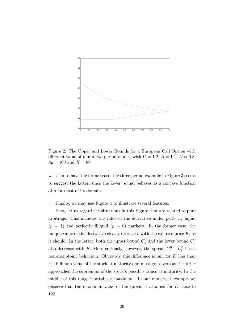
Figure 2: The Upper and Lower Bounds for a European Call Option withdifferent value of p in a two period model, with U = 1.2, R = 1.1, D = 0.8,S0 = 100 and K = 80.

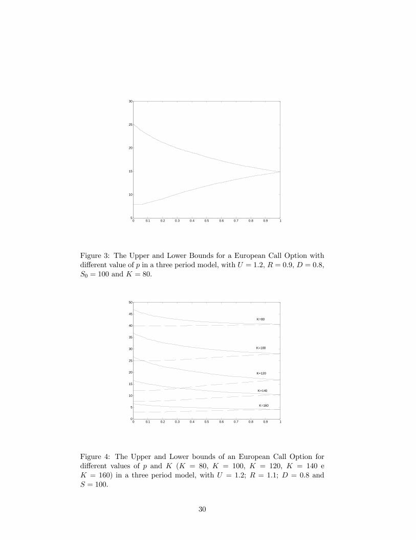
we seem to have the former case, the three period example in Figure 3 seems

to suggest the latter, since the lower bound behaves as a concave function

of p for most of its domain.

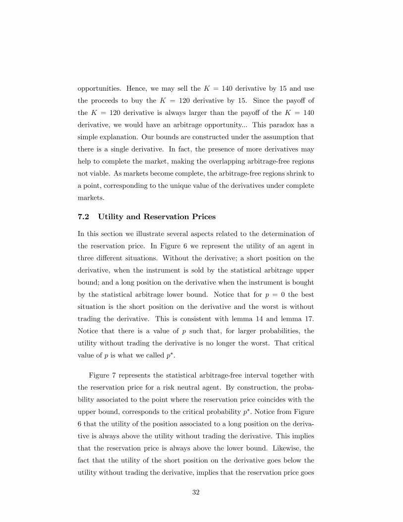
Finally, we may use Figure 4 to illustrate several features.

First, let us regard the situations in this Figure that are related to pure

arbitrage. This includes the value of the derivative under perfectly liquid

(p = 1) and perfectly illiquid (p = 0) markets. In the former case, the

unique value of the derivative clearly decreases with the exercise price K, as

it should. In the latter, both the upper bound C0u and the lower bound C0l

also decrease with K. More curiously, however, the spread C0u − C0l has anon-monotonic behaviour. Obviously this difference is null for K less than

the infimum value of the stock at maturity and must go to zero as the strike

approaches the supremum of the stock’s possible values at maturity. In the

middle of this range it attains a maximum. In our numerical example we

observe that the maximum value of the spread is attained for K close to

120.

29

0 0.1 0.2 0.3 0.4 0.5 0.6 0.7 0.8 0.9 15

10

15

20

25

30

Figure 3: The Upper and Lower Bounds for a European Call Option withdifferent value of p in a three period model, with U = 1.2, R = 0.9, D = 0.8,S0 = 100 and K = 80.

0 0.1 0.2 0.3 0.4 0.5 0.6 0.7 0.8 0.9 10

5

10

15

20

25

30

35

40

45

50

K=80

K=100

K=120

K=140

K=160

Figure 4: The Upper and Lower bounds of an European Call Option fordifferent values of p and K (K = 80, K = 100, K = 120, K = 140 eK = 160) in a three period model, with U = 1.2; R = 1.1; D = 0.8 andS = 100.

30

40 60 80 100 120 140 160 180-2

0

2

4

6

8

10

12

14

16

p=0

p=1

Figure 5: The Spread (Cu − Cl) of an European Call Option for differentvalues of K and p (p = 0, . . . , 1 with increments of 0.1) in a three periodmodel, with U = 1.2; R = 1.1; D = 0.8 and S = 100.

Regarding the statistical arbitrage domain when p ∈ (0, 1) , we noticethat all the above remarks remain true. The Figure also suggests that, for

any given p, the spread attains its maximum for the same value of K as

before. Notice that the spread Cu − Cl decreases with p for fixed strike Kconverging to zero as p → 1. Hence, although somehow different from the

traditional definition of arbitrage, the notion of statistical arbitrage seems

to provide a very nice bridge, for 0 < p < 1, between the two extreme cases

above (p = 0 and p = 1), where the original concept of arbitrage makes

sense. This can be seen in figure 5.

A third issue driven by the figure is the remark that, for intermediate

values of K, there is an overlapping of the different spreads C0u − C0l . TakeK = 120 and K = 140, for instance, when p = 0. The upper bound for

K = 140 is above the lower bound of the K = 120 derivative. The value 15

is in-between. The spread is constructed in a way such that if the K = 120

derivative is transacted by 15, there are no arbitrage opportunities. But,

if the K = 140 derivative is transacted by 15, there are also no arbitrage

31

opportunities. Hence, we may sell the K = 140 derivative by 15 and use

the proceeds to buy the K = 120 derivative by 15. Since the payoff of

the K = 120 derivative is always larger than the payoff of the K = 140

derivative, we would have an arbitrage opportunity... This paradox has a

simple explanation. Our bounds are constructed under the assumption that

there is a single derivative. In fact, the presence of more derivatives may

help to complete the market, making the overlapping arbitrage-free regions

not viable. As markets become complete, the arbitrage-free regions shrink to

a point, corresponding to the unique value of the derivatives under complete

markets.

7.2 Utility and Reservation Prices

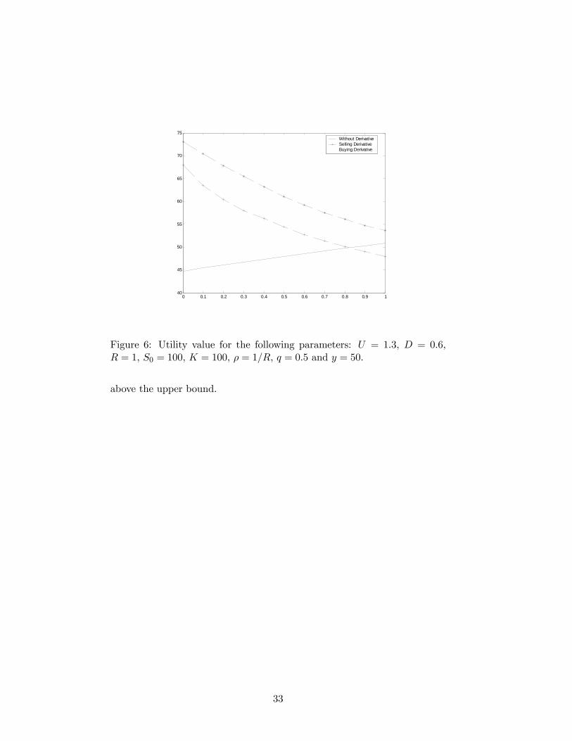
In this section we illustrate several aspects related to the determination of

the reservation price. In Figure 6 we represent the utility of an agent in

three different situations. Without the derivative; a short position on the

derivative, when the instrument is sold by the statistical arbitrage upper

bound; and a long position on the derivative when the instrument is bought

by the statistical arbitrage lower bound. Notice that for p = 0 the best

situation is the short position on the derivative and the worst is without

trading the derivative. This is consistent with lemma 14 and lemma 17.

Notice that there is a value of p such that, for larger probabilities, the

utility without trading the derivative is no longer the worst. That critical

value of p is what we called p∗.

Figure 7 represents the statistical arbitrage-free interval together with

the reservation price for a risk neutral agent. By construction, the proba-

bility associated to the point where the reservation price coincides with the

upper bound, corresponds to the critical probability p∗. Notice from Figure

6 that the utility of the position associated to a long position on the deriva-

tive is always above the utility without trading the derivative. This implies

that the reservation price is always above the lower bound. Likewise, the

fact that the utility of the short position on the derivative goes below the

utility without trading the derivative, implies that the reservation price goes

32

0 0.1 0.2 0.3 0.4 0.5 0.6 0.7 0.8 0.9 140

45

50

55

60

65

70

75Without DerivativeSelling DerivativeBuying Derivative

Figure 6: Utility value for the following parameters: U = 1.3, D = 0.6,R = 1, S0 = 100, K = 100, ρ = 1/R, q = 0.5 and y = 50.

above the upper bound.

33

0 0.1 0.2 0.3 0.4 0.5 0.6 0.7 0.8 0.9 10

5

10

15

20

25

30

35

40

45

50

Reservation Selling PriceReservation Buying PriceUpper BoundLower Bound

Figure 7: Statistical Arbitrage free bounds and reservation prices for thefollowing parameters: U = 1.3, D = 0.6, R = 1, S0 = 100, K = 100,ρ = 1/r, q = 0.5 and y = 40.

8 Conclusion

In this paper we have characterized the statistical arbitrage-free bounds for

the value of an option written on an asset that may not be transacted.

This statistical arbitrage-free interval is by construction tighter than the

usual arbitrage-free interval, obtained under the superreplication strategy.

In that sense, our result is close to the results of Bernardo and Ledoit (2000)

and Cochrane and Saá-Requejo (2000). By using a concept of statistical ar-

bitrage, in the spirit of Bondarenko’s (2003), we were able to avoid the arbi-

trary threshold that led the former approaches to constrain the arbitrage-free

interval.

In a framework characterized by the fact that transactions of the un-

derlying asset are possible with a given probability, we derived the range of

variation for the statistical arbitrage-free value of an European derivative.

If transactions were possible at all points in time there would be a unique

arbitrage-free value for the European derivative that is contained in the sta-

tistical arbitrage-free range. Moreover, the statistical arbitrage-free range is

34

contained in the arbitrage-free range of variation if the market is perfectly

illiquid. The upper bound is a decreasing function in the probability of ex-

istence of the market and the lower bound is a increasing function. They

are asymptotically well behaved both when p→ 0 and when p→ 1.

Finally, we could also prove that, in the case of random illiquidity, the

reservation prices (both for selling and buying positions) are contained in

the statistical arbitrage-free range of variation for the value of the European

Option.

35

References

[1] Amaro de Matos, J. and P. Antão, 2001, “Super-Replicating Bounds

on European Option Prices when the Underlying Asset is Illiquid”,

Economics Bulletin, 7, 1-7.

[2] Bernardo, A. and Ledoit, O., 2000, Gain, Loss, and Asset Pricing,

Journal of Political Economy, 108, 1, 144-172.

[3] Bondarenko, O., 2003, Statistical Arbitrage and Securities Prices, Re-

view of Financial Studies, 16, 875-919.

[4] Cochrane, J. and Saá-Requejo, J., 2000, Beyond Arbitrage: Good-Deal

Asset Price Bounds in Incomplete Markets, Journal of Political Econ-

omy, 108, 1, 79-119.

[5] Edirisinghe, C., V. Naik and R. Uppal, 1993, Optimal Replication of

Options with Transaction Costs and Trading Restrictions, Journal of

Financial and Quantitative Analysis, 28, 117-138.

[6] El Karoui, N. and M.C. Quenez, 1991, Programation Dynamique et

évaluation des actifs contingents en marché incomplet, Comptes Ren-

dues de l’ Academy des Sciences de Paris, Série I, 313, 851-854

[7] El Karoui, N. and M.C. Quenez, 1995, Dynamic programming and

pricing of contingent claims in an incomplete market, SIAM Journal

of Control and Optimization, 33, 29-66.

[8] Hansen. L.P. and R. Jagannathan. Implications of Security Market Data

for Models of Dynamic Economies. Journal of Political Economy, 99,

225-262, 1991.

[9] Karatzas, I. and S. G. Kou, 1996, On the Pricing of Contingent Claims

with Constrained Portfolios, Annals of Applied Probability, 6, 321-369.

[10] Longstaff, F., 1995, How Much Can Marketability Affect Security Val-

ues?, The Journal of Finance, 50, 1767—1774.

36

[11] Longstaff, F., 2001, Optimal Portfolio Choice and the Valuation of Illiq-

uid Securities, Review of Financial Studies, 14, 407-431.

[12] Longstaff, F., 2004, The Flight-to-Liquidity Premium in U.S. Treasury

Bond Prices, Journal of Business, 77, 3.

[13] Mas-Colell, A., Whiston, M. and Green, J., 1995, Microeconomic The-

ory, Oxford University Press.

37

A Some Proofs on the Solution of the Upper Boundfor Statistical Arbitrage Opportunities

A.1 Proof of theorem 10

Proof. For any given path m ∈ Ω+it,iT let λ(iT ,T ),m(it,t)

be the dual variable

associated with the superreplication constraint

Epxt,Tit

hXs=t,... ,t0−1

pxt,t0¡xt,t0 = s

¢ h∆iss S

it0 +R

t0−sBiss

ii≥³SiTT −K

´+with ik ∈ Iik+1k and k = t, . . . , T − 1. Let niTt be the number of nodes that

are predecessors of node iT at time t where niTt is given by

niTt = min T − (iT − 1) , iT − 1, T − t+ 1

At each node it that is a predecessor of iT there are #³Ω+it,iT

´.

For any given pathm ∈ Ω+it,it0 let α(it0 ,t

0),m(it,t)

be the dual variable associated

with the self-financing constraints

Epxt,t0

it

h∆ixxt,t0S

it0 +R

t0−xBixxt,t0

i−³∆it0t0 S

it0t0 +B

it0t0

´≥ 0.

Considering nit0t be the number of nodes that are predecessors of node it0 at

time t we have

nit0t = min

©t0 − (it0 − 1) , it0 − 1, t0 − t

ª+ 1

At each node it that is a predecessor of it0 there are #³Ω+it,it0

´.

The problem that must be solved in order to find the upper bound of

the range of variation of the arbitrage-free value of an European derivative

is a linear programming problem. Its dual problem is

minλiT

T+1Xj=1

λiThSiTT −K

i+where λiT is the sum of the dual variables associated with the positive ex-

pected payoff constraints that have the right member equal tohSiTT −K

i+=£

UT+1−iTDiT−1S0 −K¤+, i.e.,

λiT =T−1Xt=0

Xit:it∈It

Xnm∈Ω+it,iT

o λ(iT ,T ),m(it,t)SiTT

38

The first set of constraints is of nonnegativity of each dual variable, i.e,

λ(iT ,T ),m(it,t)

,α(it0 ,t

0),m(it,t)

≥ 0. The other set of constraints consists of equality con-straints, one constraint associated with each variable of the primal problem.

As there are

2XT−1

t=0(t+ 1) = 2

1 + (T − 1 + 1)2

T = T (T + 1)

primal variables there are also T (T + 1) constraints of the dual problem,

which are equality constraints because the variables of the primal problem

are free.

The constraint for ∆0 is:

px0,T (x0,T = 0)

∙PiT∈IT

Pm∈Ω+i0,iT

λ(iT ,T ),m(i0,0)

SiTT

¸+ α

(1,1)(i0,0)

S11 + α(2,1)(i0,0)

S21

+PT−1t=2

½Qt−1j=1 py (yj = 0)

Pnit:i0∈Iit0

o Pm∈Ω+i0,it

α(it,t),m(i0,0)

Sitt

¾= S0

The constraint for B0 is:

px0,T (x0,T = 0)RTPiT∈IT

Pm∈Ω+i0,iT

λiT ,mi0+R

³α(1,1)(i0,0)

+ α(2,1)(i0,0)

´+PT−1t=2

½Qt−1j=1 py (yj = 0)R

tPn

it:i0∈Iit0o P

m∈Ω+i0,itα(it,t),m(i0,0)

¾= 1

For the constraint that concerns ∆ik the term in λ is

px0,T (x0,T = k)Pm∈Ω+i0k,iT

PniT :i0∈I

iT0

o λ(iT ,T ),m(i0,0)SiTT +

px1,T (x1,T = k)Pn

i1:i1∈Iik1

o Pnm∈Ω+i1,iT :ik∈m

o PniT :ik∈I

iTk

o λ(iT ,T ),m(i1,1)SiTT

....

pxt,T (xt,T = k)Pn

it:it∈Iikt

o Pnm∈Ω+it,iT :ik∈m

o PniT :ik∈I

iTk

o λ(iT ,T ),m(it,t)SiTT =Pk

t=0

∙pxt,T (xt,T = k)

Pnm∈Ω+it,iT :ik∈m

o Pnit:it∈I

ikt

o PniT :ik∈I

iTk

o λ(iT ,T ),m(it,t)SiTT

¸

The terms that involve α arePt<k

Pt0>k

∙pxt,t0

¡xt,t0 = k

¢Pnit:it∈I

ikt

o Pnm∈Ω+it,it :ik∈m

o α(it0 ,t0),m(it,t)Sit0t0

¸−

−Pt<k

Pnit:it∈I

ikt

o α(ik,k),m(it,t)Sikk = 0.

39

Hence, the constraint for ∆ik isPkt=0

∙pxt,T (xt,T = k)

PniT :ik∈I

iTk

o Pnit:it∈I

ikt

o Pnm∈Ω+it,iT :ik∈m

o λ(iT ,T ),m(it,t)

SiTT

¸+P

t<k

Pt0>k

∙pxt,t0

¡xt,t0 = k

¢Pnit:it∈I

ikt

o Pnm∈Ω+it,it :ik∈m

o α(it0 ,t0),m(it,t)Sit0t0

¸+

−Pt<k

Pnit:it∈I

ikt

o α(ik,k),m(it,t)Sikk = 0

The constraint for Bik is:Pkt=0

∙pxt,T (xt,T = k)

Pnit:it∈I

ikt

o Pnm∈Ω+it,iT :ik∈m

o PniT :ik∈I

iTk

o λ(iT ,T ),m(it,t)RT−k

¸+P

t<k

Pt0>k

∙pxt,t0

¡xt,t0 = k

¢Pnit:it∈I

ikt

o Pnm∈Ω+it,it :ik∈m

o α(it0 ,t0),m(it,t)

Rt0−t¸

−Pt<k

Pnit:it∈I

ikt

o α(ik,k),m(it,t)

= 0

Note that if k = T − 1,the constraint for ∆iT−1 the constraint for ∆ik isPT−1t=0

∙pxt,T (xt,T = T − 1)

PniT :iT−1∈I

iTT−1

o Pnit:it∈I

iT−1t

o Pnm∈Ω+it,iT :iT−1∈m

o λ(iT ,T ),m(it,t)SiTT

¸+

−Pt<T−1

Pnit:it∈I

iT−1t

o α(iT−1,T−1),m(it,t)SiT−1T−1 = 0

The constraint for BiT−1 isPT−1t=0

∙pxt,T (xt,T = T − 1)

PniT :iT−1∈I

iTT−1

o Pnit:it∈I

iT−1t

o Pnm∈Ω+it,iT :iT−1∈m

o λ(iT ,T ),m(it,t)R

¸+

−Pt<T−1

Pnit:it∈I

iT−1t

o α(iT−1,T−1),m(it,t)= 0

The left member of each constraint is a linear combination of the vari-

ables of the dual problem. The right member is equal to S0 and 1 for the

dual constraints associated with the variables ∆0 and B0,respectively. For

the remaining constraints the right member is equal to zero. First, let us

consider only the constraints associated with primal variables ∆’s. For a

given iT the terms involving λ in the dual constraints regarding ∆ik is

pxt,T (xt,T = k)X

nit:it∈I

ikt

oX

nm∈Ω+it,iT :ik∈m

o λ(iT ,T ),m(it,t)SiTT

40

Summing up all the constraints that concern ∆ik with ik ∈ Ik the termassociated with and the term associated with SiT is

pxt,T (xt,T = k)X

it:it∈It

Xnm∈Ω+it,iT

o λ(iT ,T ),m(it,t)SiTT

As,

T−1Xk=t

pxt,T (xt,T = k) = 1,

summing for all k ≥ t, the term associated with SiTT that is multiplying by

pxt,T (xt,T = .) is Xit:it∈It

Xnm∈Ω+it,iT

o λ(iT ,T ),m(it,t)SiTT

Hence, summing up over all constraints associated with primal variables

∆’s we have that the terms in λ associated with SiTT are

T−1Xt=0

Xit:it∈It

Xnm∈Ω+it,iT

o λ(iT ,T ),m(it,t)SiTT

Therefore, the sum over all SiTT is

XiT :iT∈IT

T−1Xt=0

Xit:it∈It

Xnm∈Ω+it,iT

o λ(iT ,T ),m(it,t)SiTT = S0

Still considering only the constraints associated with primal variables

∆’s, in what follows we describe the terms in α. For a given Sitt , the terms

in α are

−Xs<t

Xnis:is∈Iits

o α(it,t),m(is,s)Sitt

| z from the constraint ∆it

+t−1Xk=0

t−1Xs=k

⎡⎢⎢⎣pxk,t (xk,t = s) Xnik:ik∈Iitk

oX

nm∈Ω+ik,it :is∈m

oα(it,t),m(ik,k)Sitt

⎤⎥⎥⎦| z

summing up all the constraints ∆ik , with ik ∈ Iitk

41

As,

t−1Xs=k

pxk,t (xk,t = s) = 1

the above equations sum up to zero. Summing up over all Sitt a zero will

also be obtained. Hence, if all dual constraints that concern Sitt are summed

up, the following relation is obtained:

S0 =X

iT :iT∈IT

T−1Xt=0

Xit:it∈It

Xnm∈Ω+it,iT

o λ(iT ,T ),m(it,t)SiTT (4)

Now, proceeding in a similar way but considering the dual constraints asso-

ciated with Bs. Because the right member of the constraints is equal to 0,

excepting the one associated B0, we multiply each constraint by a constant.

The constraint associated with the variable Bik is multiplied by Rk. Then,

all the constraints associated with Bs are summed up, and

XiT :iT∈IT

T−1Xt=0

Xit:it∈It

Xnm∈Ω+it,iT

o q(iT ,T ),m(it,t)= 1

where

q(iT ,T ),m(it,t)

= RT−tλ(iT ,T ),m(it,t).

Denoting,

qiT =T−1Xt=0

Xit:it∈It

Xnm∈Ω+it,iT

o q(iT ,T ),m(it,t)SiTT

equation (4) can be written as

S0 =1

RT

XiT :iT∈IT

qiTSiTT

with XiT :iT∈IT

qiT = 1

42

A.2 Proof of theorem 10 with T=3

Proof. As the problem sketched in the example of section to obtain the up-

per bound is a linear programming problem, considering Sitt = Ut−(it−1)Dit−1,

its dual is written as follows:

min½λ(iT ,T),m(it,t)

¾,

(α(it0 ,t0),m(it,t)

) ³λ(1,3)(0,0) + λ(1,3)(1,1) + λ

(1,3)(1,2)

´ £S13 −K

¤++³λ(2,3),1(0,0) + λ

(2,3),3(0,0) + λ

(2,3),3(0,0) + λ

(2,3),1(1,1) + λ

(2,3),2(1,1) + λ

(2,3)(2,1) + λ

(2,3)(1,2) + λ

(2,3)(2,2)

´ £S23 −K

¤++³λ(3,3),1(0,0) + λ

(3,3),2(0,0) + λ

(3,3),3(0,0) + λ

(3,3)(1,1) + λ

(3,3),1(2,1) + λ

(3,3),2(2,1) + λ

(3,3)(2,2) + λ

(3,3)(3,2)

´ £S33 −K

¤++³λ(4,3)(0,0) + λ

(4,3)(2,1) + λ

(4,3)(3,2)

´ £S43 −K

¤+subject to the non-negativity constraints of the dual variables

λ(iT ,T ),m(it,t)

≥ 0,

for all it ∈ IiTt , iT ∈ IT and t = 0, 1 and 2,

α(it0 ,t

0),m(it,t)

≥ 0,

for all it ∈ Iit0t , it0 ∈ It0 and t0 = 0, 1 and 2, and subject to twelve equalityconstraints, each one associated with a variable of the primal problem. The

constraint associated with ∆0 is given by

(1− p)2"λ(1,3)(0,0)S

13 +

Pm=1,2,3

λ(2,3),m(0,0) S23 +

Pm=1,2,3

λ(3,3),m(0,0) S33 + λ

(4,3)(0,0)S

43

#

+α(1,1)(0,0)S

11 + α

(2,1)(0,0)S

21+

+(1− p)hα(1,2)(0,0)

S12 +³α(2,2),1(0,0)

+ α(2,2),2(0,0)

´S23 + α

(3,2)(0,0)

S32

i= S0

(5)

The constraint associated with B0 is given by

(1− p)2R3"λ(1,3)(0,0) +

Pm=1,2,3

λ(2,3),m(0,0) +

Pm=1,2,3

λ(3,3),m(0,0) + λ

(4,3)(0,0)

#

+R³α(1,1)(0,0) + α

(2,1)(0,0)

´+ (1− p)R2

hα(1,2)(0,0) + α

(2,2),1(0,0) + α

(1,2),2(0,0) + α

(3,2)(0,0)

i= 1

(6)

43

The constraint associated with ∆11 is given by

(1− p)"λ(1,3)(1,1)S

13 +

Pm=1,2

λ(2,3),m(1,1) S23 + λ

(3,3)(1,1)S

33

#+

+p (1− p)"λ(1,3)(0,0)S

13 +

Pm=1,2

λ(2,3),m(0,0) S23 + λ

(3,3),1(0,0) S

33

#+

−α(1,1)(0,0)S11 + p

hα(1,2)(0,0)S

12 + α

(2,2),1(0,0) S

22

i+ α

(1,2)(1,1)S

12 + α

(2,2)(1,1)S

22 = 0

(7)

The constraint associated with B11 is given by

(1− p)R2"λ(1,3)(1,1) +

Pm=1,2

λ(2,3),m(1,1) + λ

(3,3)(1,1)

#+

+p (1− p)R2"λ(1,3)(0,0) +

Pm=1,2

λ(2,3),m(0,0) + λ

(3,3),1(0,0)

#+

−α(1,1)(0,0) + pRhα(1,2)(0,0) + α

(2,2),1(0,0)

i+R

hα(1,2)(1,1) + α

(2,2)(1,1)

i= 0

(8)

The constraint associated with ∆21 is given by

(1− p)"λ(2,3),3(1,1) S

23 +

Pm=1,2

λ(3,3),m(1,1) S33 + λ

(4,3)(1,1)S

43

#+

+p (1− p)"λ(2,3),3(0,0) S

23 +

Pm=2,3

λ(3,3),m(0,0) S33 + λ

(4,3)(0,0)S

43

#+

−α(2,1)(0,0)S21 + p

hα(2,2),2(0,0) S

22 + α

(3,2)(0,0)S

32

i+ α

(2,2)(2,1)S

22 + α

(3,2)(2,1)S

32 = 0

(9)

The constraint associated with B21 is given by

(1− p)R2"λ(2,3),3(1,1) +

Pm=1,2

λ(3,3),m(1,1) + λ

(4,3)(1,1)

#+

+p (1− p)R2"λ(2,3),3(0,0) +

Pm=2,3

λ(3,3),m(0,0) + λ

(4,3)(0,0)

#+

−α(2,1)(0,0)+ pR

hα(2,2),2(0,0)

+ α(3,2)(0,0)

i+R

hα(2,2)(2,1)

+ α(3,2)(2,1)

i= 0

(10)

44

The constraint associated with ∆12 is given by

λ(1,3)(1,2)U

3S0 + λ(2,3)(1,2)U

2DS0 + p³λ(1,3)(1,1)U

3S0 + λ(2,3),1(1,1) U

2DS0

´+p³λ(1,3)(0,0)

U3S0 + λ(2,3),1(0,0)

U2DS0

´− α

(1,2)(0,0)

U2S0 − α(1,2),1(1,1)

U2S0 = 0

(11)

The constraint associated with B12 is given by

Rhλ(1,3)(1,2) + λ

(2,3)(1,2)

i+ pR

hλ(1,3)(1,1) + λ

(2,3),1(1,1)

i+pR

hλ(1,3)(0,0) + λ

(2,3),1(0,0)

i− α

(1,2),1(0,0) − α

(1,2)(1,1) = 0

(12)

The constraint associated with ∆22 is given by

λ(2,3)(2,2)S

23 + λ

(3,3)(2,2)S

33 + p

h³λ(2,3),2(1,1) + λ

(2,3)(2,1)

´S23 +

³λ(3,3)(1,1) + λ

(3,3),1(2,1)

´S33

i+ph³λ(2,3),2(0,0) + λ

(2,3),3(0,0)

´S23 +

³λ(3,3),1(0,0) + λ

(3,3),2(0,0)

´S33

i−hα(2,2),1(0,0) + α

(2,2),2(0,0)

iS22 −

hα(2,2)(1,1) + α

(2,2)(2,1)

iS22 = 0

(13)

The constraint associated with B22 is given by

Rhλ(2,3)(2,2) + λ

(3,3)(2,2)

i+ pR

hλ(2,3),2(1,1) + λ

(2,3)(2,1) + λ

(3,3)(1,1) + λ

(3,3),1(2,1)

i+pR

hλ(2,3),2(0,0) + λ

(2,3),3(0,0) + λ

(3,3),1(0,0) + λ

(3,3),2(0,0)

i−hα(2,2),1(0,0) + α

(2,2),2(0,0)

i−hα(2,2)(1,1) + α

(2,2)(2,1)

i= 0

(14)

The constraint associated with ∆32 is given by

λ(3,3)(3,2)UD

2S0 + λ(4,3)(3,2)D

3S0 + phλ(3,3),2(2,1) UD

2S0 + λ(4,3)(2,1)D

3S0

i+phλ(3,3),3(0,0) UD

2S0 + λ(4,3)(0,0)D

3S0

i− α

(3,2)(0,0)D

2S0 − α(3,2)(1,1)D

2S0 = 0

(15)

The constraint associated with B32 is given by

Rhλ(3,3)(3,2) + λ

(4,3)(3,2)

i+ pR

hλ(3,3),2(2,1) + λ

(4,3)(2,1)

i+

+pRhλ(3,3),3(0,0) + λ

(4,3)(0,0)

i− α

(3,2)(0,0) − α

(3,2)(1,1) = 0

(16)

45

Summing up equations (5), (7), (9), (11),(13) and (15) we obtain

S0 =³λ(1,3)(0,0) + λ

(1,3)(1,1) + λ

(1,3)(1,2)

´S13+

+

à Pm=1,2,3

λ(2,3),m(0,0) +

Pm=1,2

λ(2,3),m(1,1) + λ

(2,3)(2,1) + λ

(2,3)(1,2) + λ

(2,3)(2,2)

!S23

+

à Pm=1,2,3

λ(3,3),m(0,0) + λ

(3,3)(1,1) +

Pm=1,2

λ(3,3),m(2,1) + λ

(3,3)(2,2) + λ

(3,3)(3,2)

!S33

+³λ(4,3)(0,0) + λ

(4,3)(2,1) + λ

(4,3)(3,2)

´S43

(17)

Multiplying equations (8) and (10) by R and equations (12), (14) and

(15) by R2 and then summing up with equation (6) we obtain

λ(1,3)(0,0) +

Pm=1,2,3

λ(2,3),m(0,0) +

Pm=1,2,3

λ(3,3),m(0,0) + λ

(4,3)(0,0)+

λ(1,3)(1,1)

+P

m=1,2λ(2,3),m(1,1)

+ λ(3,3)(1,1)

+ λ(2,3)(2,1)

+P

m=1,2λ(3,3),m(2,1)

+ λ(4,3)(2,1)

+

+λ(1,3)(1,2) + λ

(2,3)(1,2) + λ

(2,3)(2,2) + λ

(3,3)(2,2) + λ

(3,3)(3,2) + λ

(4,3)(3,2) =

1R3

Hence, denoting

q(it0 ,t

0)(it,t)

= R3λ(it0 ,t

0)(it,t)

and

q1 = q(1,3)(0,0) + q

(1,3)(1,1) + q

(1,3)(1,2)

q2 =P

m=1,2,3q(2,3),m(0,0) +

Pm=1,2

q(2,3),m(1,1) + q

(2,3)(2,1) + q

(2,3)(1,2) + q

(2,3)(2,2)

q3 =P

m=1,2,3q(3,3),m(0,0) + q

(3,3)(1,1) +

Pm=1,2

q(3,3),m(2,1) + q

(3,3)(2,2) + q

(3,3)(3,2)

q4 = q(4,3)(0,0)

+ q(4,3)(2,1)

+ q(4,3)(3,2)

we can rewrite (17) as

S0 =1R3

£q1S13 + q

2S23 + q3S33 + q

4S43¤

with qi are defied above and q1 + q2 + q3 + q4 = 1.

Taking into consideration equation (10), equation (9) can be rewritten

as

S12 =1

R

hπ(1,3)(1,2)

S13 + π(2,3)(1,2)

S23

i46

where

π(1,3)(1,2) =

λ(1,3)(1,2)

+pλ(1,3)(1,1)

+pλ(1,3)(0,0)

λ(1,3)(1,2)

+pλ(1,3)(1,1)

+pλ(1,3)(0,0)

+λ(2,3)(1,2)

+pλ(2,3),1(1,1)

+pλ(2,3),1(0,0)

π(2,3)(1,2) =

λ(2,3)(1,2)

+pλ(2,3),1(1,1)

+pλ(2,3),1(0,0)

λ(1,3)(1,2)

+pλ(1,3)(1,1)

+pλ(1,3)(0,0)

+λ(2,3)(1,2)

+pλ(2,3),1(1,1)

+pλ(2,3),1(0,0)

and π(1,3)(1,2) + π

(2,3)(1,2) = 1. Proceeding in an analogous way with constraints

(13), (14), (15) and (16) we obtain

S22 =1

R

hπ(2,3)(2,2)S

23 + π

(3,3)(2,2)S

33

iwhere

π(2,3)(2,2) =

λ(2,3)(2,2)

+p³λ(2,3),2(1,1)

+λ(2,3)(2,1)

+λ(2,3),2(0,0)

+λ(2,3),3(0,0)

´λ(2,3)(2,2)

+p³λ(2,3),2(1,1)

+λ(2,3)(2,1)

+λ(2,3),2(0,0)

+λ(2,3),3(0,0)

´+λ

(3,3)(2,2)

+p³λ(3,3)(1,1)

+λ(3,3),1(2,1)

+λ(3,3),1(0,0)

+λ(3,3),2(0,0)

´π(3,3)(2,2) =

λ(3,3)(2,2)

+p³λ(3,3)(1,1)

+λ(3,3),1(2,1)

+λ(3,3),1(0,0)

+λ(3,3),2(0,0)

´λ(2,3)(2,2)

+p³λ(2,3),2(1,1)

+λ(2,3)(2,1)

+λ(2,3),2(0,0)

+λ(2,3),3(0,0)

´+λ

(3,3)(2,2)

+p³λ(3,3)(1,1)

+λ(3,3),1(2,1)

+λ(3,3),1(0,0)

+λ(3,3),2(0,0)

´

with π(2,3)(2,2) + π

(3,3)(2,2) = 1, and

S32 =1

R

hπ(3,3)(3,2)S

33 + π

(4,3)(3,2)S

43

iwhere

π(3,3)(3,2) =

λ(3,3)(3,2)

+p³λ(3,3),2(2,1)

+λ(3,3),3(0,0)

´λ(3,3)(3,2)

+p³λ(3,3),2(2,1)

+λ(3,3),3(0,0)

´+λ

(4,3)(3,2)

+p³λ(4,3)(2,1)

+λ(4,3)(0,0)

´π(4,3)(3,2) =

λ(4,3)(3,2)

+p³λ(4,3)(2,1)

+λ(4,3)(0,0)

´λ(3,3)(3,2)

+p³λ(3,3),2(2,1)

+λ(3,3),3(0,0)

´+λ

(4,3)(3,2)

+p³λ(4,3)(2,1)

+λ(4,3)(0,0)

´with π

(3,3)(3,2) + π

(4,3)(3,2) = 1.

Moreover, using equations (7), (8), (9) and (10) we have

S11 =1

R2

hθ(1,3)(1,1)S

13 + θ

(2,3)(1,1)S

23 + θ

(3,3)(1,1)S

33

i+1

R

hε(1,2)(1,1)S

12 + ε

(2,2)(1,1)S

22

iwhere

θ(1,3)(1,1) =

R2h(1−p)λ(1,3)

(1,1)+p(1−p)λ(1,3)

(0,0)

iΘ

θ(2,3)(1,1) =

R2

"(1−p)

Pm=1,2

λ(2,3),m(1,1)

+p(1−p)P

m=1,2λ(2,3),m(0,0)

#Θ

θ(3,3)(1,1) =

R2h(1−p)λ(3,3)

(1,1)+p(1−p)λ(3,3),1

(0,0)

iΘ

ε(1,2)(1,1) =

Rhpα

(1,2)(0,0)

+α(1,2)(1,1)

iΘ , ε

(2,2)(1,1) =

Rhpα

(2,2),1(0,0)

+α(2,2)(1,1)

iΘ

47

Θ = R2h(1− p)λ(1,3)(1,1) + p (1− p)λ

(1,3)(0,0)

i+R2

⎡⎣(1− p) Xm=1,2

λ(2,3),m(1,1) + p (1− p)

Xm=1,2

λ(2,3),m(0,0)

⎤⎦+R2

h(1− p)λ(3,3)(1,1) + p(1− p)λ

(3,3),1(0,0)

i+R

hpα

(1,2)(0,0) + α

(1,2)(1,1) + pα

(2,2),1(0,0) + α

(2,2)(1,1)

iand

S21 =1

R2

hθ(1,3)(2,1)

S23 + θ(2,3)(2,1)

S33 + θ(3,3)(2,1)

S43

i+1

R

hε(1,2)(2,1)

S22 + ε(2,2)(2,1)

S32

i, with

θ(1,3)(2,1) =

R2h(1−p)λ(2,3),3

(1,1)+p(1−p)λ(2,3),3

(0,0)

iΥ

θ(2,3)(2,1) =

R2

"(1−p)

Pm=1,2

λ(3,3),m(1,1)

+p(1−p)P

m=2,3λ(3,3),m(0,0)

#Υ

θ(3,3)(2,1) =

R2h(1−p)λ(4,3)

(1,1)+pλ

(4,3)(0,0)

(1−p)i

Υ

ε(1,2)(2,1) =

Rhpα

(2,2),2(0,0)

+α(2,2)(2,1)

iΥ , ε(2,2)(2,1) =

Rhpα

(3,2)(0,0)

+α(3,2)(2,1)

iΥ

Υ = R2h(1− p)λ(2,3),3(1,1) + p (1− p)λ(2,3),3(0,0)

i+R2

⎡⎣(1− p) Xm=1,2

λ(3,3),m(1,1) + p (1− p)

Xm=2,3

λ(3,3),m(0,0)

⎤⎦++R2

h(1− p)λ(4,3)(1,1)

+ pλ(4,3)(0,0)

(1− p)i+R

hpα

(2,2),2(0,0)

+ α(2,2)(2,1)

+ pα(3,2)(0,0)

+ α(3,2)(2,1)

i.

A.3 Upper Bound for T=2

For T = 2 the problem that must be solved to find the upper bound of the

arbitrage free range of variation is the following

Cu = min∆0,B0,∆1

1,B11 ,∆

21,B

21∆0S0 +B0

subject to the conditions of positive expected payoff at time t = 0,

48

p¡∆11U

2S0 +RB11

¢+ (1− p)

¡∆0U

2S0 +R2B0

¢≥

¡U2S0 −K

¢+(18)

p¡∆11UDS0 +RB

11

¢+ (1− p)

¡∆0UDS0 +R

2B0¢≥ (UDS0 −K)+

p¡∆21UDS0 +RB

21

¢+ (1− p)

¡∆0D

2S0 +R2B0

¢≥ (UDS0 −K)+

p¡∆21D

2S0 +RB21

¢+ (1− p)

¡∆0D

2S0 +R2B0

¢≥

¡D2S0 −K

¢+(19)

positive expected payoff at time t = 1,¡∆11U

2S0 +RB11

¢≥

¡U2S0 −K

¢+¡∆11UDS0 +RB

11

¢≥ (UDS0 −K)+ (20)¡

∆21UDS0 +RB21

¢≥ (UDS0 −K)+ (21)¡

∆21D2S0 +RB

21

¢≥

¡D2S0 −K

¢+and self-financing,

∆11US0 +B11 ≤ ∆0US0 +RB0 (22)

∆21DS0 +B21 ≤ ∆0DS0 +RB0. (23)

Construct the Lagrangean

L = ∆0S0 +B0 +

+λ(1,2)(0,0)

h¡U2S0 −K

¢+ − p ¡∆11U2S0 +RB11¢− (1− p) ¡∆0U2S0 +R2B0¢i++λ

(2,2),1(0,0)

£(UDS0 −K)+ − p

¡∆11UDS0 +RB

11

¢− (1− p)

¡∆0UDS0 +R

2B0¢¤

+λ(2,2),2(0,0)

£(UDS0 −K)+ − p

¡∆21UDS0 +RB

21

¢− (1− p)

¡∆0D

2S0 +R2B0

¢¤+λ

(3,2)(0,0)

h¡D2S0 −K

¢+ − p ¡∆21D2S0 +RB21¢− (1− p) ¡∆0D2S0 +R2B0¢i+α

(2,1)(0,0)

£∆11US0 +B

11 −∆0US0 −RB0

¤+α

(1,1)(0,0)

£∆21DS0 +B

21 − (∆0DS0 +RB0)

¤+λ

(1,2)(1,1)

h¡U2S0 −K

¢+ − ¡∆11U2S0 +RB11¢i+λ

(2,2)(1,1)

£(UDS0 −K)+ −

¡∆11UDS0 +RB

11

¢¤+λ

(2,2)(2,1)

£(UDS0 −K)+ −

¡∆21UDS0 +RB

21

¢¤+λ

(3,2)(2,1)

h¡D2S0 −K

¢+ − ¡∆21D2S0 +RB21¢i49

The solution is characterized by

λ(2,2),1(0,0) = λ

(2,2),2(0,0) = λ

(1,2)(1,1) = λ

(3,2)(2,1) = 0

and

λ(1,2)(0,0),λ

(3,2)(0,0),α

(2,1)(0,0),α

(1,1)(0,0),λ

(2,2)(1,1),λ

(2,2)(2,1) ≥ 0

Using the fact that equations (18), (19), (22), (23), (20) and (21) are

binding the optimal values ∆∗0, B∗0 , ,∆

1∗1 , B

1∗1 ,∆

2∗1 , B

2∗1 can be obtained. In

particular, ∆∗0 e B∗0 are given by

∆∗0 =

¡U2S0 −K

¢+ h(U −R) (R−D) + p (R−D)2

iS0Λ

(24)

−¡D2S0 −K

¢+ h(U −R) (R−D) + p (R− U)2

iS0Λ

−p (UDS0 −K)+£−2DR+ 2RU +D2 − U2

¤S0Λ

B∗0 = −

¡U2S0 −K

¢+ hD2 (U −R) (R−D) + pUD (R−D)2

iR2Λ

+

¡D2S0 −K

¢+ hU2 (U −R) (R−D) + pUD (R− U)2

iR2Λ

+pR (UDS0 −K)+

¡−2DU2 +RU2 −RD2 + 2D2U

¢R2Λ

where

Λ = U2£(U −R) (R−D)− p

¡−R2 + 4RD −DU

¢¤−D2

£(U −R) (R−D)− p

¡−R2 − UD + 4RU

¢¤The remaining equations are also satisfied.

As a result, after some trivial algebra, we obtain

Cu = ∆∗0S0 +B

∗0 =

1

R2

hq1¡U2S0 −K

¢++ q2 (UDS0 −K)+ + q3

¡D2S0 −K

¢+i

50

with

q1 =(U −R) (R−D)

¡R2 −D2

¢+ p (R−D)2

¡R2 − UD

¢Λ

q2 = p(R−D)2

¡U2 −R2

¢+ (R− U)2

¡R2 −D2

¢Λ

q3 =(U −R) (R−D)

¡U2 −R2

¢+ p (R− U)2

¡UD −R2

¢Λ

It is easy to check that q1, q2, q3 ≥ 0 and q1 + q + q3 = 1.

A.4 Proofs of the Properties and Examples

A.4.1 Property 3

1. Proof. Let the set of admissible solutions that characterize the upper

bound for the case p ∈ (0, 1) be denoted by A (p) ,where A (p) is acorrespondence such that

A (p) : [0, 1]→ Rt(t+1).

The portfolio (∆, B) = (∆it , Bit)it∈It, t=0,... ,T−1 ∈ Rt(t+1) is said to

be an admissible solution for the problem defined in section 4.1.1 if

(∆, B) ∈ A (p) .

Moreover, let A (p = 0) and A (p = 1) denote, respectively, the admis-sible solutions for the problems characterizing the upper bound in the

case p = 0 and p = 1, presented in section 2.1.

By the Theorem of the Maximum,13 if the constraint correspondence

A (p) is continuous and if the objective function is continuous on p,then the value of the objective function in the optimum is also contin-

uous on p.

First consider the case p→ 1. In this case, limp→1A (p) = A (p = 1) .Hence,

limp→1

Cpu = Cpu (p = 1) = C

1u.

13See, for instance, Mas-Collel et al. (1995), page 963.

51

However, the same does not apply when p→ 0. In this case

limp→0

A (p) ⊆ A (p = 0)

which implies that

Cpu (p = 0) ≥ C0u.

However, using property 1, we conclude Cpu (p = 0) = C0u.

Example 21 (for T=2.) When p → 0, which means that the market is

completely illiquidity, the optimal values of ∆0 and B0 in expression (24)

converge to

∆∗0 =

¡U2S0 −K

¢+ − ¡D2S0 −K¢+S0 [U2 −D2]

B∗0 =U2¡D2S0 −K

¢+ −D2 ¡U2S0 −K¢+R2 (U2 −D2)

then,

limp→0

Cpu = ∆∗0S0 +B∗0

=1

R2

∙µR2 −D2U2 −D2

¶¡U2S0 −K

¢++

µU2 −R2U2 −D2

¶¡D2S0 −K

¢+¸,

i.e., limp→0Cpu = C0u. On the other hand, when p → 1, which means that

there is no illiquidity, the optimal values of ∆0 and B0 in expression (24)

converge to

∆∗0 =

¡U2S0 −K

¢+(R−D)−

¡D2S0 −K

¢+(U −R) + (UDS0 −K)+ (U − 2R+D)

S0R (U −D)2

B∗0 = − D (R−D)R2 (U −D)2

¡U2S0 −K

¢++

U (U −R)R2 (U −D)2

¡D2S0 −K

¢++[−D (U −R) + U (R−D)]

R2 (U −D)2(UDS0 −K)+

then,

limp→0

Cpu = ∆∗0S0 +B∗0

=1

R2

2Xj=0

µ2

j

¶µR−DU −D

¶j µU −RU −D

¶2−j ¡U jDT−jS0 −K

¢+,

i.e., limp→0Cpu = C1u.

52

A.4.2 Property 4

Proof. Consider the trading strategy¡∆∗t , B

∗t

¢t=0,... ,T−1 that solves the

maximization problem that characterizes the upper bound for a p ∈ (0, 1) .Fix a given path w, such that (it)t=0,... ,T ∈ w. For each path we have T

superreplicating constraints, one for each t ∈ 0, . . . , T − 1 . For T − 1,

∆∗iT−1SiTT +RB∗iT−1 ≥

³SiTT −K

´+,

for t = T − 2

(1− p)³∆∗iT−2S

iTT +R2B∗iT−2

´+ p

³∆∗iT−1S

iTT +RB∗iT−1

´≥³SiTT −K

´+,

which can be rewritten as

(1− p)∙∆∗iT−2S

iTT +R2B∗iT−2 −

³SiTT −K

´+¸+ p

∙∆∗iT−1S

iTT +RB∗iT−1 −

³SiTT −K

´+¸≥ 0;

for t = T − 3

(1− p)2³∆∗iT−3S

iTT +R3B∗iT−3

´+ p (1− p)

³∆∗iT−2S

iTT +R2B∗iT−2

´+

+£p (1− p) + p2

¤ ³∆∗iT−1S

iTT +RB∗iT−1

´≥³SiTT −K

´+,

which can be rewritten as

(1− p)2∙∆∗iT−3S

iTT +R3B∗iT−3 −

³SiTT −K

´+¸+ p

∙∆∗iT−1S

iTT +RB∗iT−1 −

³SiTT −K

´+¸+p (1− p)

∙∆∗iT−2S

iTT +R2B∗iT−2 −

³SiTT −K

´+¸≥ 0,

More generally, for t

Eit = Eit+1 + (1− p)T−t−1³∆∗itS

iTT +RT−tB∗it

´+

− (1− p)T−t−1³∆∗it+1S

iTT +RT−tB∗it+1

´= Eit+1 + (1− p)T−t−1

h³∆∗itS

iTT +RT−tB∗it

´−³∆∗it+1S

iTT +RT−tB∗it+1

´i≥ 0

By backward induction since T = t−1,we can prove that Eit+1 is positive.Hence, if Eit is positive for a given p it will also be positive for another p,

53

because when p increases (1− p)T−t−1 decreases. Hence, whatever the signof ³

∆∗itSiTT +RT−tB∗it

´−³∆∗it+1S

iTT +RT−tB∗it+1

´Eit will remain positive.

The same applies for the self-financing conditions.

A.4.3 Property 5

The upper bound of the ask price in a complete market can be written as

C1u =1

R2

hπliq1

¡U2S0 −K

¢++ πliq2 (UDS0 −K)+ + πliq3

¡D2S0 −K

¢+i

with

πliq1 =(R−D)2

(U −D)2

πliq1 =(R−D) (U −R)

(U −D)2

πliq1 =(U −R)2

(U −D)2

and the upper bound of the ask price in an illiquid market can be written

as

C0u =1

R2

hπilliq1

¡U2S0 −K

¢++ πilliq3

¡D2S0 −K

¢+iwith

πilliq1 =R2 −D2U2 −D2

πilliq3 =U2 −R2U2 −D2

Hence, the upper bound for the ask price in a random dry market can

be written

Cpu = αC1u + (1− α)C0u (25)

54

with

α = p

R(U−D)2(U−R)(U+D)(R−D)

1 + ph

R(U−D)2(U−R)(U+D)(R−D) − 1

i1− α =

1− p1 + p

hR(U−D)2

(U−R)(U+D)(R−D) − 1i

Taking the derivative of α with respect to p we obtain

∂α

∂p=

R (U −D)2 (R+D) (U −R) (U +D)¡R2 −D2

¢n(U −R) (U +D) (R2 −D2) + p

h(R−D)2 U (R+D) + (U −R)2D (R+D)

io2 ≥ 0

Hence, taking the derivative of C0u with respect to p we conclude that

C0u is a decreasing function of p,

∂Cpu∂p

=∂α

∂pC1u −

∂α

∂pC0u

=∂α

∂p

¡C1u − C0u

¢≤ 0.

Taking the second derivative we can also conclude that Cpu is a convex func-

tion with respect to p,

∂2Cpu∂p2

=∂2α

∂p2C1u −

∂2α

∂p2C0u

=∂2α

∂p2¡C1u − C0u

¢as

∂2α

∂p2≤ 0

we have

∂2Cpu∂p2

≥ 0.

Alternative proof: After some algebra we obtain that following relation

between α, in equation (25) and p:

α > p

55

So, as

Cask liq0 − Cask illiq0 ≤ 0

we obtain,

(p− α)³Cask liq0 −Cask illiq0

´≥ 0

pCask liq0 + (1− p)Cask illiq0 −hαCask liq + (1− α)Cask illiq

i≥ 0

and follows that

Cask0 ≤ pCask liq0 + (1− p)Cask illiq0 .

B Some Proofs on the Solution of the Lower Boundfor Statistical Arbitrage Opportunities

B.1 Proof of theorem 12

Proof. The problem that must be solved in order to find the upper bound of

the range of variation of the arbitrage-free value of an European derivative

is a linear programming problem. Its dual problem is

maxλiT

T+1Xj=1

λiThSiTT −K

i+where λiT is the sum of the dual variables associated with the positive ex-

pected payoff constraints that have the right member equal tohSiTT −K

i+=£

UT+1−iTDiT−1S0 −K¤+, i.e.,

λiT =T−1Xt=0

Xit:it∈It

Xnm∈Ω+it,iT

o λ(iT ,T ),m(it,t)SiTT

The first set of constraints is of nonnegativity of each dual variable, i.e,

λ(iT ,T ),m(it,t)

,α(it0 ,t

0),m(it,t)

≥ 0. The other set of constraints consists of equality con-straints, one constraint associated with each variable of the primal problem.

The other set are equality constraints which are equal to the ones obtained

for the upper bound. Using the same argument as in the proof of theorem

1 the proof is straightforward.

56

B.2 Lower Bound for T=2

For T = 2 the problem that must be solved to find the lower bound of the

arbitrage free range of variation is the following

Cl = max∆0,B0,∆1

1,B11 ,∆

21,B

21∆0S0 +B0

subject to the conditions of positive expected payoff at time t = 0,

p¡∆11U

2S0 +RB11

¢+ (1− p)

¡∆0U

2S0 +R2B0

¢≤

¡U2S0 −K

¢+p¡∆11UDS0 +RB

11

¢+ (1− p)

¡∆0UDS0 +R

2B0¢≤ (UDS0 −K)+

p¡∆21UDS0 +RB

21

¢+ (1− p)

¡∆0D

2S0 +R2B0

¢≤ (UDS0 −K)+

p¡∆21D

2S0 +RB21

¢+ (1− p)

¡∆0D

2S0 +R2B0

¢≤

¡D2S0 −K

¢+positive expected payoff at time t = 1,

¡∆11U

2S0 +RB11

¢≤

¡U2S0 −K

¢+¡∆11UDS0 +RB

11

¢≤ (UDS0 −K)+¡

∆21UDS0 +RB21

¢≤ (UDS0 −K)+¡

∆21D2S0 +RB

21

¢≤

¡D2S0 −K

¢+and self-financing,

∆11US0 +B11 ≥ ∆0US0 +RB0

∆21DS0 +B21 ≥ ∆0DS0 +RB0.

57

The Lagrangean of the problem is

L = ∆0S0 +B0 +

+λ(1,2)(0,0)

h¡U2S0 −K

¢+ − p ¡∆11U2S0 +RB11¢− (1− p) ¡∆0U2S0 +R2B0¢i++λ

(2,2),1(0,0)

£(UDS0 −K)+ − p

¡∆11UDS0 +RB

11

¢− (1− p)

¡∆0UDS0 +R

2B0¢¤

+λ(2,2),2(0,0)

£(UDS0 −K)+ − p

¡∆21UDS0 +RB

21

¢− (1− p)

¡∆0D

2S0 +R2B0

¢¤+λ

(3,2)(0,0)

h¡D2S0 −K

¢+ − p ¡∆21D2S0 +RB21¢− (1− p) ¡∆0D2S0 +R2B0¢i+α

(2,1)(0,0)

£∆11US0 +B

11 −∆0US0 −RB0

¤+α

(1,1)(0,0)

£∆21DS0 +B

21 − (∆0DS0 +RB0)

¤+λ

(1,2)(1,1)

h¡U2S0 −K

¢+ − ¡∆11U2S0 +RB11¢i+λ

(2,2)(1,1)

£(UDS0 −K)+ −

¡∆11UDS0 +RB

11

¢¤+λ

(2,2)(2,1)

£(UDS0 −K)+ −

¡∆21UDS0 +RB

21

¢¤+λ

(3,2)(2,1)

h¡D2S0 −K

¢+ − ¡∆21D2S0 +RB21¢iThe constraints that are binding depend on the value of the parameters.

First, if R2 − UD < 0 and p > UD−R2UD−R2+R(U−D)or R

2 − UD > 0 and p >R2−UD

R2−UD+R(U−D) the optimal solution of the dual problem is characterized by

λ(1,2)(0,0)

= λ(3,2)(0,0)

= λ(2,2)(1,1)

= λ(2,2)(2,1)

= 0

and

λ(2,2),1(0,0) ,λ

(2,2),2(0,0) ,α

(2,1)(0,0),α

(1,1)(0,0),λ

(1,2)(1,1),λ

(3,2)(2,1) ≥ 0.

Second, if R2−UD < 0 and p < UD−R2UD−R2+R(U−D) the optimal solution of the

dual problem is characterized by

λ(1,2)(0,0) = λ

(2,2),1(0,0) = λ

(1,2)(1,1) = λ

(2,2)(1,1) = α

(1,1)(0,0) = 0

and

λ(2,2),2(0,0) ,λ

(3,2)(0,0),α

(2,1)(0,0),λ

(2,2)(2,1),λ

(3,2)(2,1) ≥ 0.

Finally, if R2−UD > 0 and p < R2−UDR2−UD+R(U−D) the optimal solution of the

dual problem is characterized by

λ(2,2),2(0,0) = λ

(3,2)(0,0) = λ

(2,2)(2,1) = λ

(3,2)(2,1) = α

(2,1)(0,0) = 0

58

and

λ(1,2)(0,0),λ

(2,2),1(0,0) ,α

(1,1)(0,0),λ

(1,2)(1,1),λ

(2,2)(1,1) ≥ 0.

Hence, after some algebra the lower bound can be written as:

Cl = q1£U2S0 −K

¤++ q2 [UDS0 −K]+ + q3

£U2S0 −K

¤+(26)

with

q1 =(R−D)2

¡UD −R2

¢+ p (U −R) (R−D)

¡D2 −R2

¢R2h(U −R)2 (D2 − UD) + (R−D)2 (UD −D2) + p (U −R) (R−D) (D2 − U2)

iq2 =

(U −R)2¡D2 −R2

¢+ (R−D)2

¡R2 − U2

¢R2h(U −R)2 (D2 − UD) + (R−D)2 (UD −D2) + p (U −R) (R−D) (D2 − U2)

iq3 =

(U −R)2¡R2 − UD

¢+ p (U −R) (R−D)

¡R2 − U2

¢R2h(U −R)2 (D2 − UD) + (R−D)2 (UD −D2) + p (U −R) (R−D) (D2 − U2)

iif R2 − UD < 0 and p > UD−R2

UD−R2+R(U−D)or R2 − UD > 0 and p >

R2−UDR2−UD+R(U−D) ,

Cl =1

R2

∙R2 −D2D (U −D) [UDS0 −K]

+ +UD −R2D (U −D)

£D2S0 −K

¤+¸(27)

if R2 − UD < 0 and p < UD−R2UD−R2+R(U−D) and

Cl =1

R2

∙R2 − UDU (U −D)

£U2S0 −K

¤++

U2 −R2U (U −D) [UDS0 −K]

+

¸(28)

if R2 − UD > 0 and p < R2−UDR2−UD+R(U−D) .

B.3 Proofs of the Properties and Example

The proofs are analogous to the ones presented in appendix A.4 for the

upper bound.

B.3.1 Property 3

Example 22 (for T=2) When p → 0, which means that the market is

completely illiquidity, the values of the lower bound are given by (27) or (28)

depending on R2 − UD ≶ 0. These values coincide with the ones presented

59

in (2) for T=2. On the other hand, when p→ 1, which means that there is

no illiquidity, the values of q1, q2 and q3 presented in (26) tend to

limp→1

q1 =(R−D)2

¡UD −R2

¢+ (U −R) (R−D)

¡D2 −R2

¢R2 (U −R)2 (D2 − UD) +R2 (R−D)2 (UD − U2) +R2 (U −R) (R−D) (D2 − U2)

=(R−D)2

R2 (U −D)2

limp→1

q2 =(U −R)2

¡D2 −R2

¢+ (R−D)2

¡R2 − U2

¢R2 (U −R)2 (D2 − UD) +R2 (R−D)2 (UD −D2) +R2 (U −R) (R−D) (D2 − U2)

= 2(R−D) (U −R)R2 (U −D)2

limp→1

q3 =(U −R)2

¡R2 − UD

¢+ (U −R) (R−D)

¡R2 − U2

¢R2 (U −R)2 (D2 − UD) +R2 (R−D)2 (UD −D2) +R2 (U −R) (R−D) (D2 − U2)(U −R)2

R2 (U −D)2

then,

limp→0

Cl =(R−D)2

R2 (U −D)2£U2S0 −K

¤++ 2

(R−D) (U −R)R2 (U −D)2

[UDS0 −K]+

+(U −R)2

R2 (U −D)2£U2S0 −K

¤+which coincides with Cl, presented in equation (1).

60