Random and Deterministic DigitPermutations of the Halton Sequence*

Giray Ökten, Manan Shah, Yevgeny Goncharov

Department of Mathematics, Florida State University, Tallahassee FL 32312

Abstract

The Halton sequence is one of the classical low-discrepancy sequences. It is e¤ec-tively used in numerical integration when the dimension is small, however, for largerdimensions, the uniformity of the sequence quickly degrades. As a remedy, gener-alized (scrambled) Halton sequences have been introduced by several researcherssince the 1970s. In a generalized Halton sequence, the digits of the original Haltonsequence are permuted using a carefully selected permutation. Some of the permu-tations in the literature are designed to minimize some measure of discrepancy, andsome are obtained heuristically.

In this paper, we investigate how these carefully selected permutations di¤er froma permutation simply generated at random. We use a recent genetic algorithm, testproblems from numerical integration and computational �nance, and a recent ran-domized quasi-Monte Carlo method, to compare generalized Halton sequences withrandomly chosen permutations, with the traditional generalized Halton sequences.Numerical results suggest that the random permutation approach is as good as, orbetter than, the "best" deterministic permutations.

Key words: Halton sequence, scrambled and generalized Halton sequences, MonteCarlo, quasi-Monte Carlo

Introduction

The Halton sequences are arguably the best known and most studied low-discrepancy sequences. They are obtained from one-dimensional van der Cor-put sequences which have a simple and easy to implement de�nition. The nthterm of the van der Corput sequence in base b, denoted by �b(n), is de�ned

* This material is based upon work supported by the National Science Foundationunder Grant No. DMS 0703849.

Preprint submitted to Elsevier Science 30 January 2009

as follows: First, write n in its base b expansion:

n = (ak � � � a1a0)b = a0 + a1b+ :::+ akbk;

then compute

�b(n) = (0:a0a1 � � � ak)b =a0b+a1b2+ :::+

akbk+1

: (1)

The Halton sequence in the bases b1; :::; bs is (�b1(n); :::; �bs(n))1n=1: This is a

uniformly distributed mod 1 (u.d. mod 1) sequence (see Niederreiter [11] forits de�nition) if the bases are relatively prime. In practice, bi is usually chosenas the ith prime number.

One useful application of the Halton sequences (in general, low-discrepancysequences) is to numerical integration. The celebrated Koksma-Hlawka in-equality states,

Theorem 1 If f has bounded variation V (f) in the sense of Hardy andKrause over [0; 1]s; then, for any x1; :::; xN 2 [0; 1)s; we have����� 1N

NXn=1

f(xn)�Z[0;1)s

f(x)dx

����� � V (f)D�N(xi): (2)

For the de�nition of bounded variation in the sense of Hardy and Krause,see Niederreiter [11]. The term D�

N(xi); called the star-discrepancy of vectorsx1; :::; xN in [0; 1)s; is de�ned as follows: For a subset S of [0; 1)s; let AN(S) bethe number of vectors xi that belong to S; and let �(S) be the s-dimensionalLebesgue measure of S.

De�nition 2 The star-discrepancy of vectors x1; :::; xN 2 [0; 1)s is

D�N(xi) = sup

S

�����AN(S)N� �(S)

�����where S is an s-dimensional interval of the form

sQi=1[0; �i); and the supre-

mum is taken over the family of all such intervals. If the supremum is taken

over intervals of the formsQi=1[�i; �i); then we obtain the so-called (extreme)

discrepancy.

The star-discrepancy of the Halton sequence, or any low-discrepancy sequence,is O(N�1(logsN)): This fact, together with the Koksma-Hlawka inequality, laythe foundation of the quasi-Monte Carlo integration.

There is a well-known defect of the Halton sequence: in higher dimensionswhen the base is larger, certain components of the sequence exhibit very poor

2

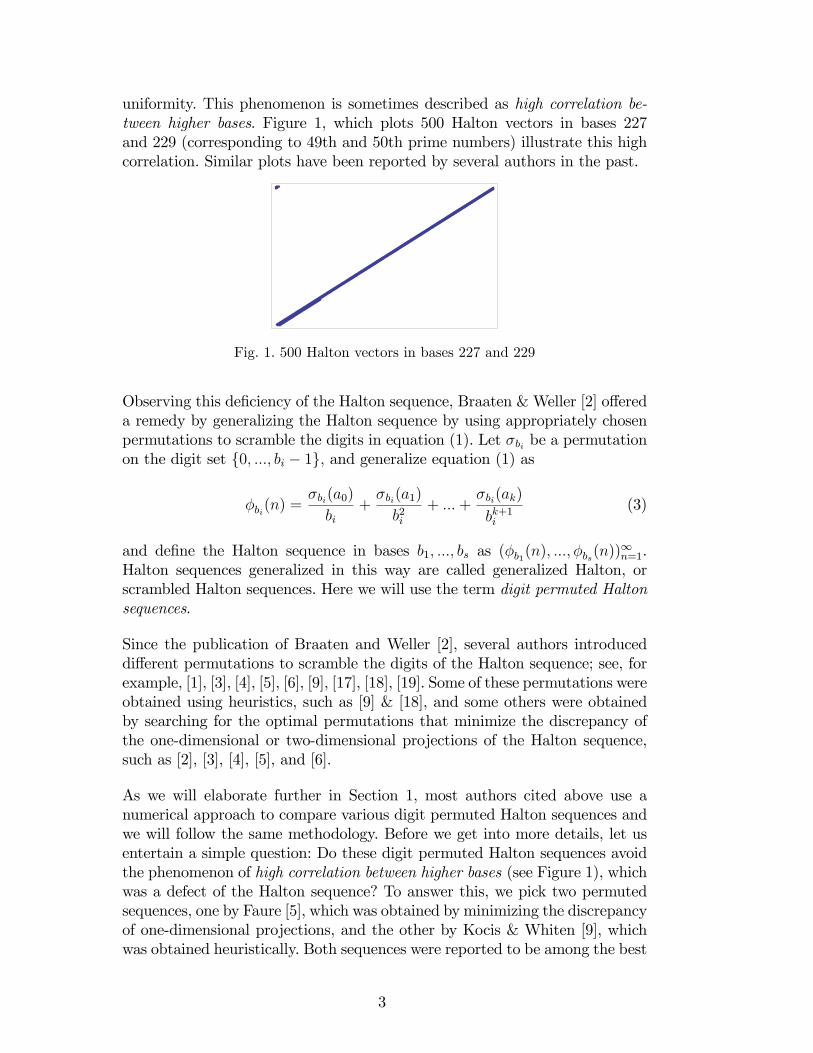
uniformity. This phenomenon is sometimes described as high correlation be-tween higher bases. Figure 1, which plots 500 Halton vectors in bases 227and 229 (corresponding to 49th and 50th prime numbers) illustrate this highcorrelation. Similar plots have been reported by several authors in the past.

Fig. 1. 500 Halton vectors in bases 227 and 229

Observing this de�ciency of the Halton sequence, Braaten & Weller [2] o¤ereda remedy by generalizing the Halton sequence by using appropriately chosenpermutations to scramble the digits in equation (1). Let �bi be a permutationon the digit set f0; :::; bi � 1g; and generalize equation (1) as

�bi(n) =�bi(a0)

bi+�bi(a1)

b2i+ :::+

�bi(ak)

bk+1i

(3)

and de�ne the Halton sequence in bases b1; :::; bs as (�b1(n); :::; �bs(n))1n=1.

Halton sequences generalized in this way are called generalized Halton, orscrambled Halton sequences. Here we will use the term digit permuted Haltonsequences.

Since the publication of Braaten and Weller [2], several authors introduceddi¤erent permutations to scramble the digits of the Halton sequence; see, forexample, [1], [3], [4], [5], [6], [9], [17], [18], [19]. Some of these permutations wereobtained using heuristics, such as [9] & [18], and some others were obtainedby searching for the optimal permutations that minimize the discrepancy ofthe one-dimensional or two-dimensional projections of the Halton sequence,such as [2], [3], [4], [5], and [6].

As we will elaborate further in Section 1, most authors cited above use anumerical approach to compare various digit permuted Halton sequences andwe will follow the same methodology. Before we get into more details, let usentertain a simple question: Do these digit permuted Halton sequences avoidthe phenomenon of high correlation between higher bases (see Figure 1), whichwas a defect of the Halton sequence? To answer this, we pick two permutedsequences, one by Faure [5], which was obtained by minimizing the discrepancyof one-dimensional projections, and the other by Kocis & Whiten [9], whichwas obtained heuristically. Both sequences were reported to be among the best

3

in recent numerical work (see [6]). Figure 2 plots 500 vectors in bases 1031 and1033, for the Faure permutation, and, 191 and 193, for the Kocis & Whitenpermutation. Note that 1033 is the 174th prime number and a dimension aslarge as 174 is not uncommon, for example, in �nancial applications.

Faure. Bases 1031 & 1033 Kocis Whiten. Bases 191 & 193

Fig. 2. 500 vectors from digit permuted Halton sequences

Figure 2 suggests that the digit permuted Halton sequences are also proneto the same de�ciency of the Halton sequence. The bases used in the aboveplots were obtained by a computer search, and there are several other pro-jections that have a similar behavior. In Section 3, we will go further than avisual inspection, and show how such large bases in digit permuted Halton se-quences can result in high error in numerical integration. We will also computeapproximations for the star-discrepancy of 10-dimensional permuted Haltonsequences, and show how large bases result in high star-discrepancy. The al-gorithm we use to compute approximations for the star-discrepancy is a novelapproach that uses genetic algorithms (see Shah [15]). The complexity of thisalgorithm grows much slower with the dimension of the sequence, comparedto the existing algorithms.

In this paper we want to investigate the following question: What if we pickthe permutation �bi in equation (3), simply at random, from the space of allpermutations? How would this approach, which we call random digit permutedHalton sequence, compare with the existing deterministic digit permuted Hal-ton sequences? Perhaps a quick test for this idea would be to plot its vectorsthat correspond to the same bases we considered in Figure 2.

Inspecting Figure 3, we do not see a visual correlation we can speak of. More-over, the same computer search program that we used to detect correlationsin digit permuted Halton sequences did not detect similar correlations for anybases for the random digit permuted Halton sequence. On the other hand,one might wonder if these plots are too "pseudorandom like". The rest of thepaper is devoted to comparing random digit permuted sequences with their de-terministic counterparts, as well as pseudorandom numbers. We will comparethese sequences by the exact error they produce in some test problems. Wewill also apply a randomized quasi-Monte Carlo method, called random start-

4

Random permutation. Bases 1031 & 1033 Random permutation. Bases 191 & 193

Fig. 3. 500 vectors from randomly permuted Halton sequences

ing, to these sequences. This randomization method enables us to computeunbiased estimates using independently randomized, digit permuted Haltonsequences. We will discuss the details in Section 3.

Based on the numerical results we discuss in the paper, our �nal conclusionwill be perhaps quite surprising: the random digit permuted Halton sequenceis as good as the best deterministic digit permuted sequences, or better, in thetest problems. In addition, we will consider a problem arti�cially designed tomagnify the impact of the correlation between higher bases, and we will seethat the random digit permutation approach is signi�cantly better than thedeterministic permutations for this problem.

1 Methodology

There are two main approaches to decide whether a given low-discrepancysequence is better than another: theoretical, and empirical. The conventionaltheoretical approach computes upper bounds for the star-discrepancy of thesequences, and chooses the one with the smaller upper bound. The star discrep-ancy of N vectors of an s�dimensional low-discrepancy sequence is boundedby cs(logN)s + O((logN)s�1) where cs is a constant that depends on the di-mension s: The theoretical approach compares di¤erent sequences by theircorresponding cs values. There are two disadvantages of this approach. First,the upper bound for the star-discrepancy becomes very large as s and N getlarger. Comparing the star-discrepancy of di¤erent sequences by comparingthe upper bounds they satisfy becomes meaningless when these upper boundsare several orders of magnitude larger than the actual star-discrepancy.

The second disadvantage is that we do not know how tight the known boundsare for the constant cs: For example, the Halton sequence used to be consideredas the worst sequence among Faure, Sobol�, Niederreiter, and Niederreiter-Xing sequences, based on the behavior of its cs value. However, recent errorbounds of Atanassov [1] imply signi�cantly lower cs values for the Halton

5

sequence. In fact, a special case of these upper bounds, which apply to adigit-permuted Halton sequence introduced by Atanassov [1], has lower csvalues than the Faure, Sobol�, Niederreiter, and Niederreiter-Xing sequences.For details see Faure & Lemieux [6].

There are two empirical approaches used in the literature to compare low-discrepancy sequences. The �rst one is to apply the sequences to test prob-lems with known solutions, and compare the sequences by the exact errorthey produce. The test problems are usually chosen from numerical integra-tion, as well as various applications such as particle transport theory andcomputational �nance. Numerical results are sometimes surprising. For exam-ple, even though the digit-permuted Halton sequence by Atanassov [1] has thebest known bounds for its star-discrepancy, after extensive numerical results,Faure & Lemieux [6] conclude that several other digit-permuted sequences(Chi, Mascagni & Warnock [4], Faure & Lemieux [6], Kocis & Whiten [9]) areas good as the one by Atanassov [1].

The second empirical approach is to compute the discrepancy of the sequencenumerically. The star-discrepancy is di¢ cult to compute, but a variant of it,the L2� discrepancy, is somewhat easier. In some papers, the L2� discrepancyis used to compare di¤erent sequences. We will discuss a major drawback ofthis approach in the next section.

In this paper, we will use the empirical approach to compare various digitpermuted Halton sequences including the random digit permutation approach.Since it is not very practical to compare all digit permuted sequences, we willproceed as follows: Following the conclusion of Faure & Lemieux [6], we willpick the Kocis-Whiten permutation as a representative of the permutationsthat performed equally well in their numerical results. We will also consider thepermutation by Faure [5], which was used successfully in previous numericalstudies of the authors (Goncharov, Ökten, Shah [8]), and the permutationby Braaten-Weller [2]. The standard Halton sequence, and the permutationby Vandewoestyne & Cools [18], will be included in the numerical results asbenchmarks.

Our empirical approach has two components. We will compare the selecteddigit permuted sequences by computing an approximation to their star dis-crepancy, for some relatively small choices for sample size N , using a recentgenetic algorithm developed by Shah [15]. For larger sample sizes, computingthe discrepancy becomes intractable, and thus we will compare the sequencesby the exact and statistical error they produce when applied to some testproblems from numerical integration and computational �nance with knownsolutions.

The test problem we will consider from numerical integration is estimating

6

the integral of

f(x1; :::; xs) =sYi=1

j4xi � 2j+ ai1 + ai

(4)

in [0; 1)s: This function was �rst considered by Radovic, Sobol�, Tichy [14],and used subsequently by several authors. The exact value of the integral isone, and the sensitivity of the function to xi quickly decreases as ai increases.The other two test problems we will consider are from computational �nance:pricing European and ratchet options.

2 Computing the discrepancy

A modi�ed version of the star-discrepancy, which is easier to compute, is theL2-star discrepancy:

De�nition 3 The L2-star discrepancy of vectors x1; :::; xN 2 [0; 1)s is

T �N(xi) =

24Z[0;1)s

AN(S)

N� �(S)

!2d�1:::d�s

351=2

where S =sQi=1[0; �i):

Similarly, we can de�ne the L2-extreme discrepancy, TN(xi); by replacingthe sup norm in the de�nition of extreme discrepancy (De�nition 2) by theL2�norm. There are explicit formulas to compute T �N and TN of a �nite setof vectors. However, the formulas are ill-conditioned and they require highprecision; see Vandewoestyne & Cools [18] for a discussion.

A more serious drawback of the L2-discrepancies T �N and TN is that they tendto give small values when the vectors are close to the vertex (1; 1; :::; 1) of thes-dimensional cube. Moreover, as was observed by Matou�ek [10], if N is smalland s is large, the L2-discrepancy of any point set is close to the best possibleL2-discrepancy.

We now discuss a recent example where the L2-discrepancies give misleadingresults. In Vandewoestyne & Cools [18], a new permutation for the Haltonsequence, called the reverse permutation, was introduced. The authors com-pared several digit permuted Halton sequences by their T �N and TN ; in di-mensions that varied between 8 to 32. They considered at most N = 1000vectors in their computations. They concluded that the reverse permutationperformed as good, or better, than the other permutations, in terms of theL2-discrepancies. For example, Figure 9 on page 355 of [18] shows that T �N ofthe reverse permutation is much lower than the Braaten-Weller permutation,

7

as N varies between 1 and 1000. Table 1 displays T �N and D�N for these per-

mutations, for N = 10; 100; and 200: The D�N values are computed using a

genetic algorithm, which we will discuss in more detail later.

T �N D�N

N BW Reverse BW Reverse

50 13:5� 10�4 2:00� 10�4 0:295 0:404

100 7:01� 10�4 1:77� 10�4 0:261 0:356

200 3:64� 10�4 1:53� 10�4 0:152 0:268TABLE 1: T �N and D�

N

Observe that although T �N values for the reverse permutation are lower thanthe Braaten-Weller permutation for each N , exactly the opposite is true forD�N !Which one of these results indicate a better sequence in terms of numerical

integration? Next, we compare these sequences by comparing the exact errorthey produce when used to integrate the function f (see (4)). Table 2 displaysthe absolute error against the sample sample size N: The choices we make forN match the values used in Figure 9 of [18].

N Reverse BW REV/BW

100 434� 10�5 34:1� 10�5 12:7

200 138� 10�5 13:7� 10�5 10:0

300 47:4� 10�5 44:2� 10�5 1:1

400 113� 10�5 7:28� 10�5 15:5

500 18:2� 10�5 18:0� 10�5 1:0

600 17:2� 10�5 38:8� 10�5 0:4

700 66:5� 10�5 9:84� 10�5 6:8

800 37:2� 10�5 11:4� 10�5 3:3

900 8:93� 10�5 8:89� 10�5 1:0

1000 25:8� 10�5 11:8� 10�5 2:2TABLE 2: Integration error for f

We observe that except for N = 600; the Braaten-Weller permutation erroris less than or equal to the reverse permutation error. In fact, in almost all ofthe numerical results of this paper, the reverse permutation, together with thestandard Halton sequence, gave the largest error among the digit permutedsequences.

8

2.1 Computing star-discrepancy using a genetic algorithm

Here we will discuss a recent genetic algorithm by Shah [15] that computeslower bounds for the star-discrepancy. The parameters of the algorithm weredetermined so that the algorithm provides good estimates for the star dis-crepancy when applied to two types of examples. The �rst type of examplesincluded a small number of low-discrepancy vectors and dimension, so that theexact star-discrepancy could be computed using a brute force search algorithm.For example, the star-discrepancy of the �rst 50 vectors of the 5-dimensionalHalton sequence was computed using a brute force search algorithm. Then thegenetic algorithm was run, independently, forty times to obtain forty estimates(lower bounds) for the star-discrepancy. Thirty-eight of these estimates werein fact the exact discrepancy, and the remaining two were within 1.64% of theexact value.

The other type of examples Shah used to determine the algorithm parametershad larger number of vectors or dimension, and a brute force search was notpractical. However, lower and upper bounds for the star-discrepancy could becomputed using an algorithm by Thiémard [16]. Shah used the examples andthe bounds given in [16], and was able to show that the genetic algorithmconsistently yielded discrepancy estimates within Thiémard�s bounds.

In the next two tables, we compute the star-discrepancy of the �rst 100 digitpermuted Halton vectors, D�

100, using the genetic algorithm. We consider thepermutations by Vandewoestyne & Cools [18] (called reverse permutation),Faure [5], Kocis & Whiten [9], and the standard Halton sequence; these se-quences are labeled as Reverse, Faure, KW, and Halton, respectively, in thetables. We want to compare these digit permuted sequences with our proposedrandom digit permuted sequences, with respect to their star-discrepancy. Todo this, we generate forty random permutations independently, which givesforty random digit permuted Halton sequences. We then compute the star-discrepancy of the �rst 100 vectors of these sequences. The sample mean ofthe star-discrepancies of these forty sequences, together with a 95% bootstrapcon�dence interval, is reported in the last row of the tables.

In Table 3, there are three cases labeled as A, B, and C. In each case, wecompute D�

100 when the dimension of the sequence is �ve, however, di¤erentcases use di¤erent bases. In A, the bases of the Halton sequence are the �rst�ve prime numbers; p1; p2; :::; p5 (pi is the ith prime number): In B, the basesare p14;p20; p27; p33; p39; and in C the bases are p46;p47; p48; p49; p50: We would

9

like to see how increasing the prime base a¤ects the discrepancy.

D�100 Case A Case B Case C

Halton 0:110 0:601 0:961

Reverse 0:084 0:401 0:563

Faure 0:097 0:143 0:185

KW 0:100 0:149 0:124

Random 0:104 0:146 0:188

(0:101; 0:106) (0:142; 0:151) (0:181; 0:196)TABLE 3: Star-discrepancy for di¤erent bases. Dimension is �ve.

When the prime bases and the dimension (which is �ve) are low, as in CaseA, we do not expect to see the standard Halton sequence have poor star-discrepancy, and the results support that. The star-discrepancy of Halton,KW, and Random are very close. Reverse and Faure are slightly better. InCase B, we increase the prime bases, in a mixed way, and the results changeconsiderably. Now Halton is the worst, followed by Reverse. PermutationsFaure, KW, and Random are in good agreement. Further increasing the basesin Case C spreads out the values; KW gives the lowest star-discrepancy, andFaure & Random come next.

In Table 5 we repeat a similar analysis, but now the problem is slightly moredi¢ cult: the dimension of the vectors is 10. In Case A, the bases are the �rstten primes, and Halton and Reverse give the highest star-discrepancy. Faureand KW give the lowest values, followed by Random. In Case B, C, and D,the bases are the ith prime numbers where i 2 f11, 17, 21, 22, 24, 29, 31,35, 37, 40}, i 2 f41, 42, 43, 44, 45, 46, 47, 48, 49, 50}, and i 2 f43, 44, 49,50, 76, 77, 135, 136, 173, 174}. In all of these cases, Halton and Reverse givethe highest star-discrepancy values, and the others remain close to each other.Note that the Random permutation approach gives con�dence intervals thatare lower than the star-discrepancy of the best deterministic digit permutedsequences in Cases B and C. In other words, a randomly permuted sequencehas a lower star-discrepancy than the deterministic permutations we consider,

10

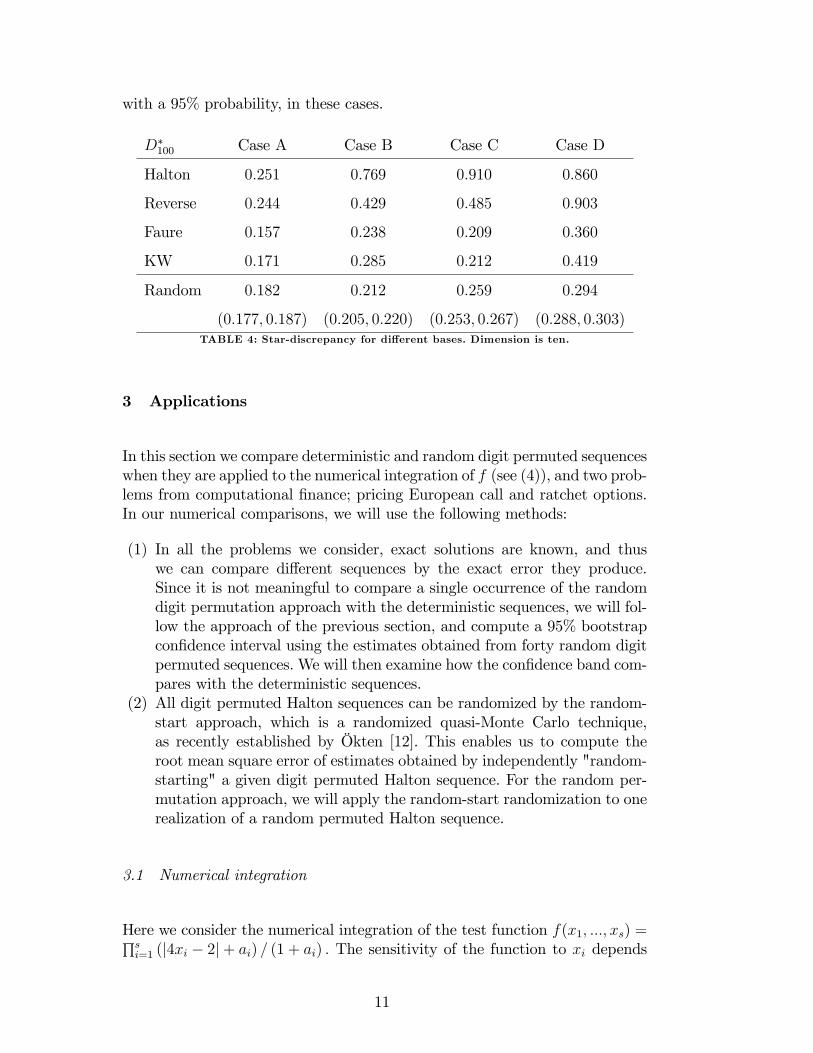
with a 95% probability, in these cases.

D�100 Case A Case B Case C Case D

Halton 0:251 0:769 0:910 0:860

Reverse 0:244 0:429 0:485 0:903

Faure 0:157 0:238 0:209 0:360

KW 0:171 0:285 0:212 0:419

Random 0:182 0:212 0:259 0:294

(0:177; 0:187) (0:205; 0:220) (0:253; 0:267) (0:288; 0:303)TABLE 4: Star-discrepancy for di¤erent bases. Dimension is ten.

3 Applications

In this section we compare deterministic and random digit permuted sequenceswhen they are applied to the numerical integration of f (see (4)), and two prob-lems from computational �nance; pricing European call and ratchet options.In our numerical comparisons, we will use the following methods:

(1) In all the problems we consider, exact solutions are known, and thuswe can compare di¤erent sequences by the exact error they produce.Since it is not meaningful to compare a single occurrence of the randomdigit permutation approach with the deterministic sequences, we will fol-low the approach of the previous section, and compute a 95% bootstrapcon�dence interval using the estimates obtained from forty random digitpermuted sequences. We will then examine how the con�dence band com-pares with the deterministic sequences.

(2) All digit permuted Halton sequences can be randomized by the random-start approach, which is a randomized quasi-Monte Carlo technique,as recently established by Ökten [12]. This enables us to compute theroot mean square error of estimates obtained by independently "random-starting" a given digit permuted Halton sequence. For the random per-mutation approach, we will apply the random-start randomization to onerealization of a random permuted Halton sequence.

3.1 Numerical integration

Here we consider the numerical integration of the test function f(x1; :::; xs) =Qsi=1 (j4xi � 2j+ ai) = (1 + ai) : The sensitivity of the function to xi depends

11

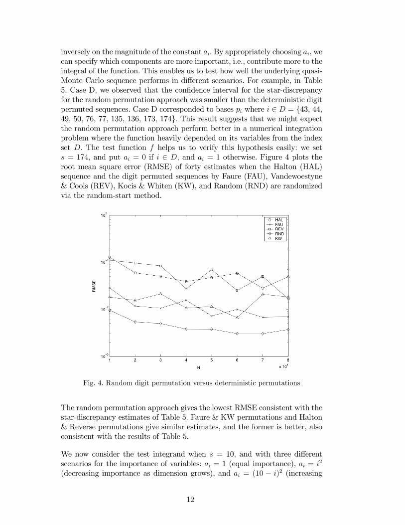
inversely on the magnitude of the constant ai: By appropriately choosing ai; wecan specify which components are more important, i.e., contribute more to theintegral of the function. This enables us to test how well the underlying quasi-Monte Carlo sequence performs in di¤erent scenarios. For example, in Table5, Case D, we observed that the con�dence interval for the star-discrepancyfor the random permutation approach was smaller than the deterministic digitpermuted sequences. Case D corresponded to bases pi where i 2 D = f43, 44,49, 50, 76, 77, 135, 136, 173, 174g: This result suggests that we might expectthe random permutation approach perform better in a numerical integrationproblem where the function heavily depended on its variables from the indexset D: The test function f helps us to verify this hypothesis easily: we sets = 174; and put ai = 0 if i 2 D; and ai = 1 otherwise. Figure 4 plots theroot mean square error (RMSE) of forty estimates when the Halton (HAL)sequence and the digit permuted sequences by Faure (FAU), Vandewoestyne& Cools (REV), Kocis & Whiten (KW), and Random (RND) are randomizedvia the random-start method.

Fig. 4. Random digit permutation versus deterministic permutations

The random permutation approach gives the lowest RMSE consistent with thestar-discrepancy estimates of Table 5. Faure & KW permutations and Halton& Reverse permutations give similar estimates, and the former is better, alsoconsistent with the results of Table 5.

We now consider the test integrand when s = 10; and with three di¤erentscenarios for the importance of variables: ai = 1 (equal importance), ai = i2

(decreasing importance as dimension grows), and ai = (10 � i)2 (increasing

12

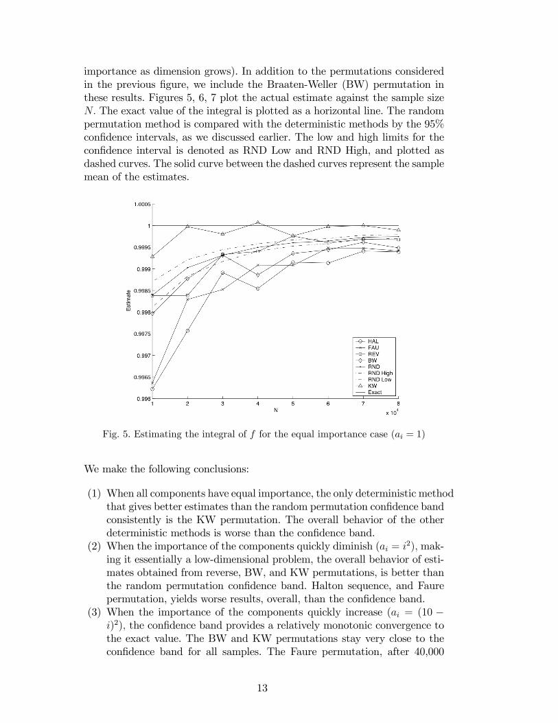
importance as dimension grows). In addition to the permutations consideredin the previous �gure, we include the Braaten-Weller (BW) permutation inthese results. Figures 5, 6, 7 plot the actual estimate against the sample sizeN: The exact value of the integral is plotted as a horizontal line. The randompermutation method is compared with the deterministic methods by the 95%con�dence intervals, as we discussed earlier. The low and high limits for thecon�dence interval is denoted as RND Low and RND High, and plotted asdashed curves. The solid curve between the dashed curves represent the samplemean of the estimates.

Fig. 5. Estimating the integral of f for the equal importance case (ai = 1)

We make the following conclusions:

(1) When all components have equal importance, the only deterministic methodthat gives better estimates than the random permutation con�dence bandconsistently is the KW permutation. The overall behavior of the otherdeterministic methods is worse than the con�dence band.

(2) When the importance of the components quickly diminish (ai = i2); mak-ing it essentially a low-dimensional problem, the overall behavior of esti-mates obtained from reverse, BW, and KW permutations, is better thanthe random permutation con�dence band. Halton sequence, and Faurepermutation, yields worse results, overall, than the con�dence band.

(3) When the importance of the components quickly increase (ai = (10 �i)2); the con�dence band provides a relatively monotonic convergence tothe exact value. The BW and KW permutations stay very close to thecon�dence band for all samples. The Faure permutation, after 40,000

13

Fig. 6. Estimating the integral of f for the diminishing importance case (ai = i2)

Fig. 7. Estimating the integral of f for the increasing importance case (ai = (10�i)2)

samples, stays close to the band as well. The estimates of the other twomethods, Halton and reverse, show an erratic behavior, and except for afew samples, have larger error.

(4) We did not include the Monte Carlo results in these �gures since theMonte Carlo error was much worse than all the other sequences: the

14

RMSE of Monte Carlo is worse by factors between approximately 10 and300 in the three cases we considered. We do not include Monte Carloresults in the rest of the section.

3.2 Pricing European options

Details of European options and the risk-free pricing by simulation can befound in Glasserman [7]. In the following, we consider a European call optionunder the lognormal model with the following parameters: exercise price is 40,volatility is 0.2, risk-free interest rate is 6%, and the expiry is 2 years. TheEuropean option can be solved as a one-dimensional problem, however, sincewe want to see the impact of high dimensions, we treat this as a path dependentoption and simulate complete price paths with a uniform discretization of100 steps. In other words, the dimension of the problem, and the underlyingsequence in simulation, is 100. We consider three values for the initial stockprice; 36, 40, and 44. For these choices, the option is called out-of-the money,at-the-money, and in-the-money. As the initial stock price increases, more ofthe price paths will contribute a non-zero value to the price of the option.

Figures 8, 9, 10 plot the root mean square error (RMSE) of forty estimates,when the random-start method is applied to the digit permuted sequencesHAL, FAU, REV, RND, and KW. In all �gures, the RMSE of HAL and REVare higher than the others approximately by factors between 10 and 20. InFigure 8, it is di¢ cult to distinguish between FAU, RND, and KW. In Figures9 & 10, the RMSE of RND is smaller than both FAU and KW in all excepttwo samples, although the improvements are relatively small.

3.3 Pricing ratchet options

Details of ratchet (digital) options can be found in Papageorgiou [13]. Herewe consider the following parameters: the initial stock price is 100, risk-freeinterest rate is 4:5%, the volatility is 0:3, and the expiry is 1. We considera uniform discretization of 64 steps, i.e., the dimension of simulation is 64.Figure 11 plots the RMSE of the forty estimates obtained via the random-start method. The results are similar to the European option example. Halton(HAL) and Reverse (REV) have larger RMSE, by approximately about factorsbetween 5 and 10. The random permutation (RND) has the lowest RMSE forall sample sizes except one.

15

Fig. 8. Pricing an out-of-the-money European call option

Fig. 9. Pricing an at-the-money European call option

4 Conclusions

Deterministic permutations designed to improve the uniformity of the Haltonsequence have been around since the 1970s. Although various numerical exper-

16

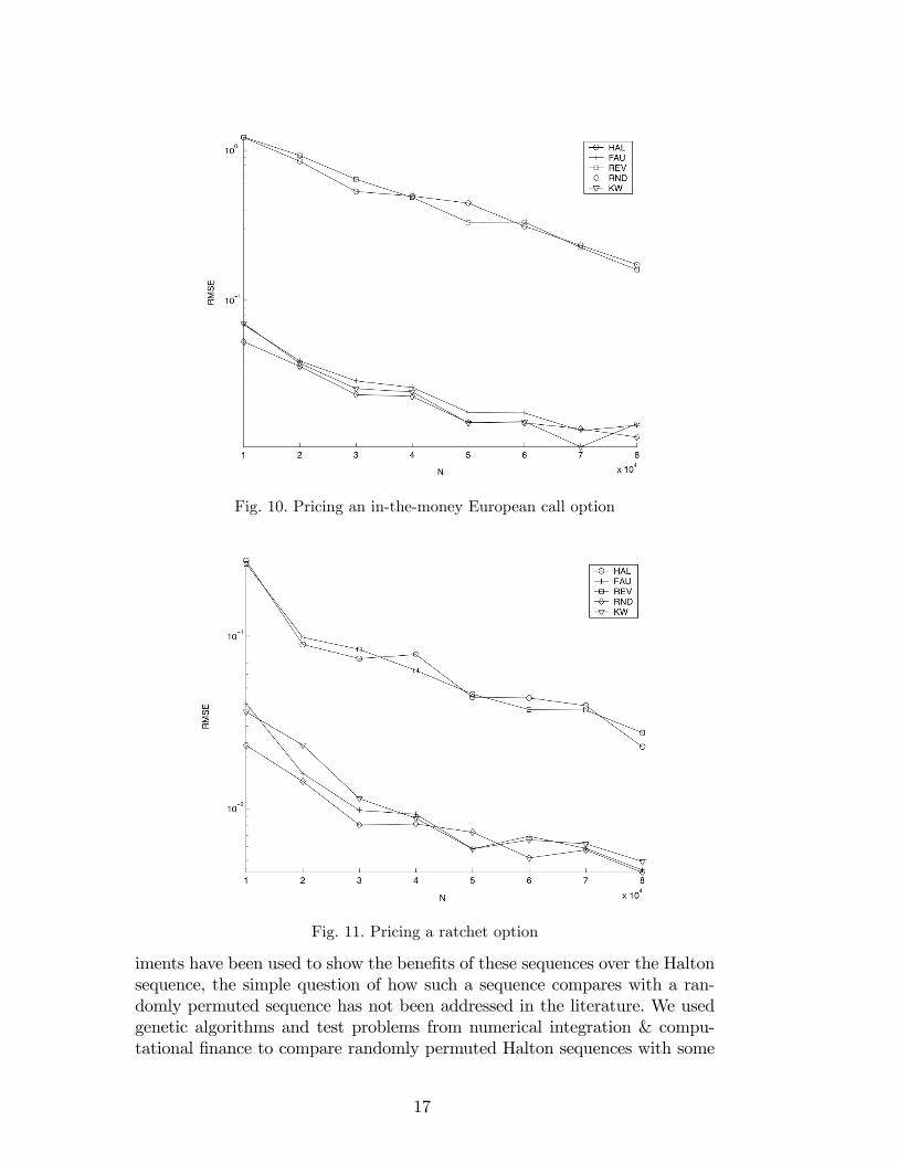
Fig. 10. Pricing an in-the-money European call option

Fig. 11. Pricing a ratchet option

iments have been used to show the bene�ts of these sequences over the Haltonsequence, the simple question of how such a sequence compares with a ran-domly permuted sequence has not been addressed in the literature. We usedgenetic algorithms and test problems from numerical integration & compu-tational �nance to compare randomly permuted Halton sequences with some

17

selected deterministic sequences. The comparison was made in two di¤erentways; by applying the random-start method which enables the computation ofmean square errors, and by constructing bootstrap con�dence intervals. Quitesurprisingly, the random permutation approach was as good as, or better,than the "best" deterministic permutations, in the problems we considered.We think further research and numerical studies are needed to understand thesurprising success of this approach.

References

[1] E. I. Atanassov, On the discrepancy of the Halton sequences, Math. Balkanica,New Series 18 (2004) 15-32.

[2] E. Braaten, G. Weller, An improved low-discrepancy sequence formultidimensional quasi-monte Carlo integration, Journal of ComputationalPhysics 33 (1979) 249-258.

[3] H. Chaix, H. Faure, Discrepance et diaphonie en dimension un, Acta ArithmeticaLXIII (1993) 103�141.

[4] H. Chi, M. Mascagni, T. Warnock, On the optimal Halton sequence,Mathematics and Computers in Simulation 70 (2005) 9-21.

[5] H. Faure, Good Permutations for Extreme Discrepancy, Journal of NumberTheory 42 (1992) 47�56.

[6] H. Faure, C. Lemieux, Generalized Halton Sequences in 2007: A ComparativeStudy, Technical report, 2007.

[7] P. Glasserman, Monte Carlo Methods in Financial Engineering, Springer-Verlag, 2004.

[8] Y. Goncharov, G. Ökten, M. Shah, Computation of the endogenous mortgagerates with randomized quasi-Monte Carlo simulations, Mathematical andComputer Modelling 46 (2007) 459-481.

[9] L. Kocis, W. J. Whiten, Computational investigations of low-discrepancysequences, ACM Transactions on Mathematical Software 23 (1997) 266-294.

[10] J. Matou�ek, On the L2-Discrepancy for Anchored Boxes, Journal of Complexity14 (1998) 527-556.

[11] H. Niederreiter. Random Number Generation and Quasi-Monte Carlo Methods,SIAM, Philadelphia, 1992.

[12] G. Ökten, Generalized von Neumann-Kakutani transformation and random-start scrambled Halton sequences, Journal of Complexity, forthcoming (availabeonline 11/24/08).

18

[13] A. Papageorgiou, The Brownian Bridge Does Not O¤er a Consistent Advantagein Quasi-Monte Carlo Integration, Journal of Complexity 18 (2002) 171-186.

[14] I. Radovic, I. M. Sobol�, R. F. Tichy, Quasi-Monte Carlo Methods for NumericalIntegration: Comparison of di¤erent low discrepancy sequences, Monte CarloMethods and Applications 2 (1996) 1-14.

[15] M. Shah, Quasi-Monte Carlo and Genetic Algorithms with Applications toEndogenous Mortgage Rate Computation, Ph.D. Dissertation, Department ofMathematics, Florida State University, 2008.

[16] E. Thiémard, An Algorithm to Compute Bounds for the Star Discrepancy,Journal of Complexity 17 (2001) 850-880.

[17] B. Tu¢ n, A new permutation choice in Halton sequences, in: Monte Carlo andQuasi-Monte Carlo 1996, Vol 127, Springer Verlag, New York, 1997, pp 427-435.

[18] B. Vandewoestyne, R. Cools, Good permutations for deterministic scrambledHalton sequences in terms of L2-discrepancy, Journal of Computational andApplied Mathematics 189 (2006) 341-361.

[19] T. T. Warnock, Computational Investigations of low-discrepancy point sets II,in: Harald Niederreiter and Peter J. -S. Shiue, editors, Monte Carlo and quasi-Monte Carlo methods in scienti�c computing, Springer, New York, 1995, pp.354-361.

19