Embed Size (px)
Citation preview

ALEXANDRIA UNIVERSITY FACULTY OF ENGINEERING
RANDOM ACCESS PROTOCOLS FOR FUTURE OPTICAL CDMA NETWORKS
A Thesis Submitted to the Electrical Engineering Department
in Partial Fulfillment of the Requirements for the Degree of
Master of Science in
Electrical Engineering
By
Ziad Ahmed Rashad El-Sahn
B.Sc. in Electrical Engineering (Communications & Electronics), June 2002
Supervisors
Prof. Dr. El-Sayed A. El-Badawy Prof. Dr. Hossam M. H. Shalaby
Electrical Engineering Department, Faculty of Engineering, Alexandria University
Registered: September 2002
Submitted: April 2005

ÉΟ ó¡ Î0 «! $# Ç⎯≈uΗ ÷q §9$# ÉΟŠ Ïm §9$#
﴿ y7Ï9≡ sŒ ã≅ôÒ sù «! $# ϵ‹ Ï?÷σム⎯ tΒ â™!$ t± o„ 4 ª! $#uρ ρèŒ È≅ôÒ xø9$# ÉΟŠ Ïà yèø9$# ﴾
٤ ، اآليةاجلمعةسورة
﴿ ≅è% uρ Éb>§‘ ’ ÎΤ ÷ŠÎ— $ Vϑù= Ïã ﴾ ١١٤، اآلية طـهسورة

EVALUATION COMMITTEE
We certify that we have read this thesis and that, in our opinion, it is fully adequate in
scope and quality as a dissertation for the degree of Master of Science in Electrical
Engineering.
Evaluation Committee Signature
- Prof. Dr. El-Sayed A. El-Badawy Department of Electrical Engineering,
Alexandria University, Alexandria, Egypt.
Higher Institute of Engineering, Thebes Academy, Cairo, Egypt.
- Prof. Dr. Hossam M. H. Shalaby Department of Electrical Engineering, Faculty of Engineering,
Alexandria University, Alexandria, Egypt.
- Prof. Dr. Moustafa Hussein Aly Department of Electronics and Communication Engineering,
Arab Academy for Science & Technology, Alexandria, Egypt.
- Prof. Dr. Diaa Abdel Meguid M. Khalil Department of Electronics and Communication Engineering,
Faculty of Engineering, Ein-Shams University, Cairo, Egypt.
For the faculty council
Prof. Dr. Ossama Rashed Vice Dean for graduate and research
Faculty of Engineering, Alexandria University.
Alexandria 21544, Egypt.

iii
SUPERVISORS
Prof. Dr. El-Sayed A. El-Badawy
Dean, Higher Institute of Engineering, Thebes Academy, Cairo 11434, Egypt.
Professor Emeritus, Department of Electrical Engineering,
Faculty of Engineering, Alexandria University,
Alexandria 21544, Egypt.
Email: [email protected]
Prof. Dr. Hossam M. H. Shalaby
Professor, Department of Electrical Engineering,
Faculty of Engineering, Alexandria University,
Alexandria 21544, Egypt.
Email: [email protected]

iv
VITAE
Personal Information
Date of Birth: 22nd November, 1979.
Place of Birth: Alexandria, Egypt.
Education
1984 – 1997 College Saint-Marc Alexandria, Egypt
Alliance Française 1996.
Diplôme de Langue Française 1997 signé par L'Ambassadeur de France.
1998 – 2002 Faculty of Engineering Alexandria University
B.Sc. in Electrical Engineering (Communications and Electronics), June 2002.
Overall Grade: Excellent with Degree of Honour.
Overall Rank: 3rd over a class of 300 students.
Graduation Project: Multimedia Mobile Communications.
Professional and Work Experience
1999 Training Arabia Computer Systems Alexandria, Egypt 2000 Training Federal Arab Maritime Company Alexandria, Egypt 2001 Training Schlumberger - Wireline Shukeir, Egypt 2002 – Present Faculty of Engineering, Alexandria University
Teaching Assistant (Full Time), Department of Electrical
Engineering, Communications and Electronics Section.

v
ACKNOWLEDGEMENTS
نحمد اهللا عز وجل أن هدانا لهذا وما آنا لنهتدي لوال أن هدانا اهللا
First, I would like to express my heartfelt gratitude to my supervisors Prof. Dr.
El-Sayed A. El-Badawy, and Prof. Dr. Hossam M. H. Shalaby, for their
academic advice, constant encouragement, guidance, and support during my
graduate school years. I am really grateful to them for contributing many
suggestions and improvements.
My appreciation also goes to my colleagues at the Department of Electrical
Engineering (Alexandria University) for the friendly academic atmosphere,
and their encouragement. In addition, I would like to express my thanks to
Eng. Yousef Abdel Malek for his help and useful discussions; I really feel so
proud working hand in hand with him all throughout the research program.
I am extremely grateful to my parents who have sacrificed themselves to give
me the best education. From my early childhood, they raised me to love
learning, and supported me to develop my interest in science and engineering.
Their unreserved love and support for these many years is what makes this
M.Sc. degree possible. I would also like to thank them for their continuous
support, for their patience, encouragement and extra care.
Thank you all.

vi
PUBLICATIONS AND AWARDS
[1] Z. A. El-Sahn, Y. M. Abdel-Malek, H. M. H. Shalaby, and El-S. A. El-Badawy,
"Performance limitations in the R3T optical random access CDMA protocol,"
Submitted for possible publication to OSA J. Optical Networking, March 2005.
This paper won the 1st position in paper evaluation and 3rd position after
presentation, IEEE Egyptian Student Branch Contest 2004, AAST, Cairo,
Egypt, January 2005.
[2] Z. A. El-Sahn, Y. M. Abdel-Malek, H. M. H. Shalaby, and El-S. A. El-Badawy,
"The R3T optical random access CDMA protocol with queuing subsystem,"
Submitted for possible publication to the IEEE/OSA J. Lightwave Technol., also a
summary submitted to the 31st European Conference on Optical Communication,
(ECOC 2005), Glasgow, Scotland, 25-29 September 2005.
[3] Z. A. El-Sahn, Y. M. Abdel-Malek, H. M. H. Shalaby, and El-S. A. El-Badawy,
"Proposed optical random access CDMA protocol with stop & wait ARQ,"
Submitted for possible publication to OSA J. Optical Networking, also a summary
submitted to the 31st European Conference on Optical Communication, (ECOC
2005), Glasgow, Scotland, 25-29 September 2005.
This paper was presented in part at the Fifth Workshop on Advanced
Photonics, The National Institute of Laser Sciences, Cairo University, Egypt,
May 2005.
[4] Z. A. El-Sahn, Y. M. Abdel-Malek, H. M. H. Shalaby, and El-S. A. El-Badawy,
"Optical random access CDMA protocol with stop & wait ARQ and a queuing
subsystem," Submitted for possible publication to OSA Optics Letters.

ABSTRACT

vii
ABSTRACT
In this thesis we present an overview on optical code division multiple access
(CDMA) communication systems. Both physical and optical link layers are studied.
Focus is oriented towards random access protocols and media access control (MAC)
protocols for future optical CDMA networks.
One of the main objectives of this research is to study the performance of the
optical CDMA round robin receiver/transmitter (R3T) protocol in noisy environments
and dispersive channels. We proved by numerical analysis that the effect of thermal
noise dominates the performance only for low population networks, whereas the
effect of multiple access interference (MAI) becomes dominant for larger networks.
We found out that there are optimum values for the operating wavelength and the
average peak laser power of the transmitter to compensate for this degradation.
Then, we suggest a queuing model to the R3T protocol in order to enhance its
performance. A detailed state diagram is outlined and a mathematical model based on
the equilibrium point analysis (EPA) technique is presented. Our results reveal that
significant improvement in terms of the steady state system throughput and the
protocol efficiency can be achieved by only adding a single buffer to the system
which does not add considerably to the network complexity. The modified protocol
significantly outperforms the R3T protocol for larger population networks and at
higher traffic loads. Furthermore, the modified R3T protocol exhibits an acceptable
timeout probability under different network parameters.
Finally, we propose an optical random access CDMA protocol based on stop
& wait automatic repeat request (ARQ). A mathematical description of this protocol is
outlined using a detailed state diagram. Several performance measures are considered;
namely, the steady state system throughput, the blocking probability, the average
packet delay, and the protocol efficiency. We proved by numerical analysis that the
proposed protocol is less complex and significantly outperforms the R3T protocol
(which is based on a go-back n technique) at higher population networks. Our results
also show that the performance of the proposed protocol with correlation receivers is
nearly close to that of the R3T protocol with chip-level receivers, which significantly
reduces the overall system cost.

viii
TABLE OF CONTENTS
TABLE OF CONTENTS viii
LIST OF FIGURES xii
LIST OF TABLES xv
LIST OF SYMBOLS xvi
ACRONYMS xix
CHAPTER 1: INTRODUCTION AND THESIS SURVEYS 1
1.1 Introduction 1
1.2 Contributions of the Thesis 2
1.3 Organization of the Thesis 3
CHAPTER 2: RESEARCH AND DEVELOPMENT IN OPTICAL
CDMA COMMUNICATION SYSTEMS
5
2.1 Introduction 5
2.2 Basic Optical CDMA Communication Systems 5
2.2.1 System Architecture 5
2.2.2 Optical Orthogonal Codes (OOCs) 6
2.3 Optical CDMA Encoding - Decoding Techniques 7
2.3.1 Time Domain Encoding Using Optical Delay Line Loops 7
2.3.2 Spectral Intensity Encoding CDMA Systems 8
2.3.3 Optical Fast Frequency Hop CDMA (FFH-CDMA) 10
2.3.4 Important Design Issues in Optical CDMA 11
2.4 Various Optical CDMA Receivers 11
2.4.1 Correlation Receivers 12
2.4.1.1 Passive Correlation Receivers 12
2.4.1.2 Active Correlation Receivers 13
2.4.1.3 Correlation Receivers with Optical Hard-Limiters 13
2.4.2 Chip-Level Receivers 15
2.4.2.1 High-Speed Chip-Level Receivers 15
2.4.2.2 All Optical Chip-Level Receivers 16
2.4.3 Comparison of Various Optical CDMA Receivers 17

ix
2.5 Performance of Optical CDMA Receivers 18
2.5.1 Correlation Receivers without Hard-Limiter 19
2.5.2 Chip-Level Receivers 20
2.5.3 Simulation Results 21
2.5.4 Conclusions 24
CHAPTER 3: OPTICAL CDMA RANDOM ACCESS PROTOCOLS
FOR FUTURE LOCAL AREA NETWORKS
25
3.1 Introduction 25
3.2 Background and Basic Information 25
3.2.1 Traditional Random Access Protocols 26
3.2.1.1 Pure ALOHA 26
3.2.1.2 Slotted ALOHA 27
3.2.1.3 CSMA and CSMA/CD 28
3.2.2 The Need for MAC Protocols for Optical Networks 28
3.3 Optical CDMA Protocols with and without Pretransmission Coordination 29
3.3.1 System Architecture 29
3.3.2 Optical CDMA Protocols' Description 30
3.3.2.1 First Protocol: Pro 1 30
3.3.2.2 Second Protocol: Pro 2 30
3.3.2.3 Variation of Pro 2 30
3.3.3 Optical CDMA Protocols' Performance 31
3.3.3.1 The Effect of MAI 31
3.3.3.2 Performance Metrics 32
3.3.4 Results and Conclusions 32
3.4 Round Robin Receiver/Transmitter (R3T) Protocol 34
3.4.1 Network and System Design 35
3.4.1.1 Physical Layer Implementation 35
3.4.1.2 Optical Link Layer 35
3.4.2 Mathematical Model and Theoretical Analysis 35
3.4.2.1 State Diagram and Protocol Description 36
3.4.2.2 Performance Evaluation 38
3.4.3 Simulation Results 40
3.4.4 Summary and Conclusions 43

x
CHAPTER 4: IMPAIRMENTS IN THE R3T OPTICAL RANDOM
ACCESS CDMA PROTOCOL
44
4.1 Introduction 44
4.2 Impairments in Fiber Optic Communication Systems 44
4.2.1 Receiver Noise 44
4.2.1.1 Shot Noise 45
4.2.1.2 Thermal Noise 45
4.2.2 Light Dispersion in Fibers 45
4.2.2.1 Modal Dispersion 46
4.2.2.2 Chromatic Dispersion 46
4.3 Performance of the R3T Protocol in a Noisy Environment 47
4.3.1 System Architecture and Hardware Implementation 48
4.3.2 Effect of Thermal Noise 48
4.3.2.1 Mathematical Analysis 48
4.3.2.2 Numerical Results 51
4.3.3 Effect of Light Dispersion 55
4.3.3.1 Mathematical Analysis 56
4.3.3.2 Numerical Results 57
4.4 Conclusions 59
CHAPTER 5: THE R3T OPTICAL RANDOM ACCESS CDMA
PROTOCOL WITH QUEUING SUBSYSTEM
60
5.1 Scope and Motivation 60
5.2 System Architecture 60
5.2.1 Optical CDMA Network 60
5.2.2 Optical CDMA Protocol 61
5.3 Mathematical Model 62
5.4 Theoretical Analysis 68
5.4.1 State Diagram Analysis 68
5.4.1.1. Transmission Mode 68
5.4.1.2. Reception Mode 70
5.4.1.3. Acknowledgement Mode 71
5.4.1.4. Requesting Mode 71
5.4.2 Performance Measures 73

xi
5.4.2.1 Steady State Throughput 73
5.4.2.2 Protocol Efficiency 74
5.4.2.3 Timeout Probability 74
5.5 Simulation Results 75
5.6 Conclusions 80
CHAPTER 6: PROPOSED OPTICAL RANDOM ACCESS CDMA
PROTOCOL WITH STOP & WAIT ARQ
81
6.1 Introduction 81
6.2 System and Hardware Architecture 82
6.3 Mathematical Model 83
6.3.1 Protocol Assumptions 83
6.3.2 State Diagram Description 84
6.4 Performance Analysis 86
6.4.1 State Diagram 86
6.4.1.1 Transmission Mode 87
6.4.1.2 Reception Mode 87
6.4.1.3 Acknowledgement Mode 88
6.4.1.4 Requesting Mode 88
6.4.2 Performance Metrics 88
6.4.2.1 Steady State System Throughput 88
6.4.2.2 Blocking Probability 89
6.4.2.3 Protocol Efficiency and Average Delay 89
6.5 Numerical Results 90
6.6 Conclusions 95
CHAPTER 7: CONCLUSIONS AND FUTURE WORK 97
7.1 Conclusions 97
7.2 Future Research Avenues 98
REFERENCES 100

xii
LIST OF FIGURES
Fig. 2.1 Optical CDMA network configuration. 6
Fig. 2.2 Time domain optical CDMA encoding of high peak intensity ultra-
short pulses using delay line loops: (a) Encoder, (b) Decoder.
8
Fig. 2.3 Spectral intensity encoded optical CDMA system: (a) Encoder, (b)
Decoder.
9
Fig. 2.4 Optical FFH-CDMA system: (a) Encoder, (b) Decoder. 10
Fig. 2.5 Passive correlator structure. 12
Fig. 2.6 Active correlator structure. 13
Fig. 2.7 Optical hard-limiters’ characteristics: (a) An ideal optical hard-
limiter, (b) A practical optical hard-limiter.
14
Fig. 2.8 (a) Optical correlation receiver with hard-limiter, (b) Optical
correlation receiver with double hard-limiters.
15
Fig. 2.9 (a) High-speed chip-level receiver, (b) All optical chip-level
receiver.
16
Fig. 2.10 Bit error probabilities for OOK-CDMA receivers, under a Poisson
shot-noise-limited assumption, versus average photons/bit.
18
Fig. 2.11 Packet success probability versus number of active users for
different packet sizes.
22
Fig. 2.12 Packet success probability versus number of active users and code
length for correlation receivers.
23
Fig. 2.13 Packet success probability versus number of active users and code
length for chip-level receivers.
23
Fig. 3.1 Normalized throughput versus offered traffic for ALOHA systems. 27
Fig. 3.2 Optical CDMA network architecture. 29
Fig. 3.3 Throughput versus average activity for different protocols. 33
Fig. 3.4 Throughput and delay versus average activity for different
protocols.
33
Fig. 3.5 Complete state diagram of the R3T optical CDMA protocol. 36
Fig. 3.6 Throughput and blocking probability versus average activity for
different number of users.
40

xiii
Fig. 3.7 Throughput and blocking probability versus number of users for
different propagation delays.
41
Fig. 3.8 Throughput and delay versus timeout duration for different
activities.
42
Fig. 4.1 Typical dispersion versus wavelength curves. 47
Fig. 4.2 Bit error probabilities for OOK-CDMA chip-level receivers versus
the decision threshold.
50
Fig. 4.3 Packet success probability and decision threshold versus the
average peak laser power and the receiver noise temperature for
different number of active users.
52
Fig. 4.4 Throughput versus average peak laser power for different
propagation delays.
53
Fig. 4.5 Packet delay versus throughput for different propagation delays. 54
Fig. 4.6 Protocol efficiency versus blocking probability for different
number of users.
55
Fig. 4.7 Throughput versus message length for different interstation
distances and wavelengths.
57
Fig. 4.8 Throughput versus user bit rate for different interstation distances. 58
Fig. 5.1 An optical CDMA network in a star configuration. 61
Fig. 5.2 Complete state diagram of the R3T optical CDMA protocol with a
single buffer in the queue.
63
Fig. 5.3 Detailed state diagram of the requesting mode. 64
Fig. 5.4 Detailed state diagram of the acknowledgement mode. 65
Fig. 5.5 Detailed state diagram of the reception mode. 66
Fig. 5.6 Detailed state diagram of the transmission mode. 67
Fig. 5.7 (a) State rn , (b) State Txt+i , (c) State WXi . 67
Fig. 5.8 Throughput versus number of users for different propagation
delays.
76
Fig. 5.9 Available packets and throughput versus average activity. 76
Fig. 5.10 Protocol efficiency versus message length for different number of
users.
77
Fig. 5.11 Timeout probability versus average activity and timeout duration. 78
Fig. 5.12 Timeout probability versus number of users. 79

xiv
Fig. 6.1 Optical CDMA network topology. 82
Fig. 6.2 State diagram of the proposed optical CDMA protocol with stop &
wait ARQ.
85
Fig. 6.3 Transmission states, Txi and reception states, Rxi. 86
Fig. 6.4 Throughput versus number of users for different receivers. 91
Fig. 6.5 Blocking probability versus user activity for different interstation
distances.
92
Fig. 6.6 Throughput and delay versus activity for different number of users
and different interstation distances.
93
Fig. 6.7 Throughput versus number of users for different interstation
distances.
94
Fig. 6.8 Efficiency versus message length for different number of users. 94
Fig. 6.9 Throughput versus number of users and average peak laser power
per chip.
95

xv
LIST OF TABLES
Table 2.1 Comparison of various optical CDMA receiver structures. 17
Table 2.2 Examples of optimal (L,3,1,1) optical orthogonal codes. 22
Table 3.1 Notations and description for states in the R3T protocol state
diagram.
37
Table 4.1 Typical values of simulation parameters. 52
Table 4.2 Light source and optical fiber specifications. 57
Table 6.1 Parameters used for numerical calculations. 90

xvi
LIST OF SYMBOLS
A Average user activity
a Acknowledgement states
C Number of pulses with θ≥iY
C Maximum achievable number of codes
c Speed of light in free space
D Average packet delay
d Average delay spent in the backlog mode
chromD Chromatic dispersion parameter
e Retransmission states
F APD excess noise factor
G Offered traffic
APDG Average APD gain
dI APD dark current
K Number of bits in a packet
k Interference vector
BK Boltzmann's constant
effk APD effective ionization ratio
L Code length
l Message length in packets
m Initial state
jbm Conditional mean of the decision variable jY
N Number of users
n number of backlogged users
1n Core refractive index
NA Numerical aperture
vaP Received average peak laser power
BP Blocking probability

xvii
cbP Conditional bit correct probability
lbP Bocklogged probability
inP Input power
outP Output power
SP Packet success probability
thP Thinking probability
otP Timeout probability
1p Probability of 1 chip interference
wp Probability of w chip interference
Q Photon count within a chip interval
)(xQ Normalized Gaussian tail probability
dQ Photon count due to dark current within a chip interval
q Requesting states
eq Magnitude of the electron charge
APDR APD responsivity at unity gain
bR User bit rate
LR Load resistor
xxR Auto-correlation function
xyR Crosscorrelation function
r Transmission states
'r Number of active users
oS Zero dispersion slope
s Reception states
T Bit duration
t Two-way propagation time
cT Chip duration oT Receiver noise temperature
sT Slot duration
u Constant output of an optical hard-limitter

xviii
v Speed of light inside a fiber
'v Threshold level of an optical hard-limiter eW Waiting after retransmission states qW Waiting after request states rW Waiting after transmission states sW Waiting after reception states
w Code weight
iY Photon count within weighted chip i
Z Total number of received pulses
z Interstation distance
β Steady state system throughput γ Probability to receive an acknowledgement
chromt∆ Pulse spreading due to chromatic dispersion
altmod∆ Pulse spreading due to modal dispersion
λ∆ Spectral line width of a light source η Protocol efficiency
θ Decision threshold
λ Wavelength
aλ Auto-correlation constraint
cλ Cross-correlation constraint
oλ Zero dispersion wavelength
nπ Stationary probabilities
σ Probability to find a connection request 2
jbσ Conditional variance of the decision variable jY
2nσ Variance of thermal noise within a chip interval
τ Timeout duration

xix
ACRONYMS
APD Avalanche Photodiode
ARQ Automatic Repeat Request
BER Bit Error Rate
CDMA Code Division Multiple Access
CLSP Channel Load Sensing Protocols
CRC Cyclic Redundancy Check
CSMA Carrier-Sense Multiple-Access
CSMA/CD CSMA with Collision Detection
DC Direct Current
EPA Equilibrium Point Analysis
FBGs Fiber Bragg Gratings
FFH-CDMA Fast Frequency Hop CDMA
FTTB Fiber To The Building
FTTC Fiber To The Curb
FTTCab Fiber To The Cabinet
FTTH Fiber To The Home
IEEE Institute of Electrical and Electronics Engineering
IM-DD Intensity Modulation and Direct Detection
ISI Intersymbol Interference
LAN Local Area Network
LED Light Emitting Diode
MAC Media Access Control
MAI Multiple Access Interference
OOCs Optical Orthogonal Codes
OOK On Off Keying
OSI Open Systems Interconnection
PAC Packet Avoidance Collision
PPM Pulse Position Modulation
QOS Quality Of Service
R3T Round Robin Receiver/Transmitter

xx
SNR Signal to Noise Ratio
WDMA Wavelength Division Multiple Access

CHAPTER 1
INTRODUCTION AND THESIS SURVEYS
Outline:
• Introduction
• Contributions of the Thesis
• Organization of the Thesis

1
CHAPTER 1
INTRODUCTION AND THESIS SURVEYS
1.1 Introduction
While applications drive the development for faster and more efficient
network technology, on the other hand network technology opens up the opportunity
for the development of new applications. Applications that were not feasible or even
imaginable a few years ago are now widely used. The most current example is the
development of multimedia applications for the World Wide Web. Web browsers
permit us to receive not only text-based information, but also audio and video from a
wide variety of sources such as research institutions, governments, businesses, and
individuals. These new applications are pushing the limits on current networks, since
they require a great amount of bandwidth and have specific quality of service (QOS)
requirements. The increasing demand makes imperative the use of some new
technology that is not only capable of meeting today's demands but is also flexible to
accommodate tomorrow's growth.
Fiber based optical communication networks offer an efficient way to meet
these requirements [1]-[8]. Therefore, optical transmission has taken over in the
backbone networks during the last decade and is continuously being deployed closer
to the edge of the networks. In the access network, there is an increased interest in
fiber to the home (FTTH), fiber to the building (FTTB), fiber to the curb (FTTC), and
fiber to the cabinet (FTTCab) technologies. For access networks and local area
networks (LANs), low cost is a very important factor and thus systems with low
complexity must be proposed.
Spread spectrum signaling has been recently proposed to achieve multi-user
capability in fiber-optic code division multiple access (CDMA) networks [9]-[11].
The main advantage of using CDMA in an optical network is that it allows a flexible
multiple access method for asynchronous traffic with a graceful degradation at high
interference. Furthermore, variable requirements on bit error rates (BER) can be
satisfied by suitable choices of codes. An additional advantage is that some processing

2
can be moved into the optical domain, which is important since certain operations can
be implemented with very low complexity using optical components. Because there
are no standards or commercial implementations available for optical CDMA
networks, the question of the best implementation method is still open. Furthermore, it
is not clear whether CDMA is a suitable solution for optical networks. According to
studies by Stok and Sargent, CDMA can offer a higher capacity than wavelength
division multiple access (WDMA) for local area networks if noise is neglected [2].
Furthermore, CDMA can be efficiently used in conjunction with WDMA on
multimedia communication networks where multiple services with different traffic
requirements are to be integrated. However, when shot noise and thermal noise are
taken into consideration, CDMA is much more sensitive to the signal to noise ratio
than WDMA [3]. Therefore, it is not clear that the comparison will hold when also
other noise types are taken into account.
One of the motivating factors for the work in this thesis was the small amount
of research concerning the network or link layer of optical CDMA communication
systems [4]-[8]. In this thesis focus will be mainly on protocols and solutions for
LANs, but many of the principles can also be used for access networks.
1.2 Contributions of the Thesis
As current network technologies evolve to an all optical largely passive
infrastructure, design and implementation problems take on new significance and
raise a number of challenging issues that require novel solutions. In [7], Shalaby has
proposed an optical random access CDMA protocol called round robin
receiver/transmitter (R3T) protocol. This protocol is based on a go back- n automatic
repeat request (ARQ) and is suitable for only low population networks. In his
analysis, Shalaby assumed that each node is equipped with a single buffer to store
only a single message (the message that is being served); thus any arrival to a
nonempty buffer was discarded. This of course gives rise to a blocking probability
which was not studied and thus limits the system throughput. Also focus was oriented
towards only multiple access interference (MAI), the effect of receiver’s noise and
other impairments were neglected.
This thesis makes the following contributions, focusing on the design and analysis of

3
MAC and link layer protocols for optical CDMA networks. The main contributions of
the thesis work can be summarized as follows:
1- Studying the impact of the receiver’s thermal noise on the performance of the
R3T protocol. Also the effect of light dispersion on limiting the user bit rate is
considered. Chip-level receivers are considered in the analysis because of their
high ability to overcome the effect of MAI.
2- Introducing a queuing subsystem to the R3T protocol, namely increasing the
number of available buffers. The steady state system throughput, the protocol
efficiency, and the timeout probability are derived, simulated and compared
with the previous results in [7]. Our results show that significant improvement
in the performance of the R3T protocol can be achieved by only adding a
single buffer to the system.
3- Developing a new optical random access CDMA protocol based on a stop &
wait ARQ. The performance of this protocol is evaluated in terms of the
system throughput, the blocking probability, the protocol efficiency, and the
average packet delay. Our results reveal that the proposed protocol
outperforms the R3T protocol in large population networks.
1.3 Organization of the Thesis
Following the introduction in Chapter 1; which summarizes the motivation,
objectives, and achievements in this research, Chapter 2 presents an overview of the
physical layer of optical CDMA communication systems. Different CDMA encoding
techniques and receiver structures are outlined. In Chapter 3, we give a quick review
for the different MAC protocols that were proposed in literature. The link layer of an
optical direct-detection CDMA packet network is then considered. Finally, we present
a mathematical analysis for several proposed random access protocols in [6] and [7].
Chapter 4 is concerned with the major sources of limitations in optical CDMA
systems. Both receiver noise and light dispersion in fibers are studied. Also the
performance of the R3T protocol in noisy environments and dispersive channels is
investigated. The performance of the R3T protocol with a queuing subsystem is
discussed in Chapter 5. A mathematical model based on the equilibrium point analysis
(EPA) is presented. In addition, the steady state system throughput, the protocol

4
efficiency, and the timeout probability are derived and evaluated under several
network parameters and compared with the results in [7]. In Chapter 6, we propose a
new optical random access CDMA protocol which is based on a stop & wait ARQ in
order to reduce the complexity of the previously proposed protocols. The performance
of this protocol is evaluated for different receiver structures and under different
network parameters. Furthermore, the effect of the receiver thermal noise is analyzed.
Finally, Chapter 7 presents the conclusions of this thesis and suggests directions for a
further research in this area.

CHAPTER 2
RESEARCH AND DEVELOPMENT IN OPTICAL
CDMA COMMUNICATION SYSTEMS
Outline:
• Introduction
• Basic Optical CDMA Communication Systems
• Optical CDMA Encoding - Decoding Techniques
• Various Optical CDMA Receivers
• Performance of Optical CDMA Receivers

5
CHAPTER 2
RESEARCH AND DEVELOPMENT IN
OPTICAL CDMA COMMUNICATION SYSTEMS
2.1 Introduction
Over the last one to two decades, there has been a lot of interest and research
in optical CDMA systems. More than 250 papers have been written in this area since
1985 [12]. A vast number of different schemes using time domain or frequency
domain encoding approaches have been proposed [13]-[17]. Coherent and non-
coherent manipulations of optical signals have been used in different proposals and
various codes have been devised for optical CDMA systems. In this chapter, we try to
give a general review of the previous work done in this field.
Also we consider different receiver structures proposed for fiber-optic CDMA
systems [18], [19] and discuss their major strengths and drawbacks. The receiver
structures introduced and studied here are those structures with minimum electronic
processing. The main electronic functions used in these structures are integration and
comparison with a threshold value. These are the simplest electronic functions that
can be implemented with relatively high speeds. Other receiver structures can be
introduced which massively benefit from electronic signal processing. Such receivers
can employ for example pattern recognition or multi-user detection techniques to
improve the performance of the systems. However, the intensive electronic processing
required is not desirable for high-speed optical CDMA signal processing due to its
complexity.
2.2 Basic Optical CDMA Communication Systems
2.2.1 System Architecture
A typical fiber-optic CDMA communication system is best represented by an
information data source followed by a laser when the information is in electrical

6
signal form, and an optical encoder that maps each bit of the output information into a
very high rate optical sequence, which is then coupled into the single-mode fiber
channel. At the receiver end, the optical pulse sequence would be compared to a
stored replica of itself (correlation process) and to a threshold level at the comparator
for the data recovery. In fiber-optic CDMA there are N such transmitter and receiver
pairs (users). Figure 2.1 shows one such network in a star configuration. The set of the
different fiber-optic CDMA pulse sequences essentially becomes a set of address
codes or signature sequences for the network. One of the primary goals of optical
CDMA is to extract data with the desired optical pulse sequence in the presence of all
other users’ optical pulse sequences.
Fig. 2.1. Optical CDMA network configuration.
2.2.2 Optical Orthogonal Codes (OOCs)
Central to any successful code division multiple-access scheme, whether
electrical or optical, is the choice of the high rate sequences; namely, the signature
sequences, on which the information data bits of different users is mapped. In CDMA,
many asynchronous users occupy the same channel simultaneously. A desired user’s
receiver must be able to extract its signature sequence in the presence of other user’s
signature sequences. Therefore, a set of signature sequences that are distinguishable
from time shifted versions of themselves and for which any two such signature
sequences are easily distinguishable from each other is needed. The design of
sequences with these properties for communication systems, such as spread-spectrum
CDMA, ranging systems, radar systems, etc., has been a topic of interest to many

7
communications scientists and mathematicians in the last two decades [20]. These
traditional codes cannot be used in optical CDMA systems. A new family of unipolar
codes named Optical Orthogonal Codes (OOCs) has been proposed for optical CDMA
systems by J. A. Salehi [9].
An optical orthogonal code is a family of (0,1) sequences with good auto- and
cross-correlation properties, i.e., the autocorrelation of each sequence exhibits the
'thumbtack' shape and the cross-correlation between any two sequences remains low
throughout. A family of OCC's is denoted by ( )cawL λλφ ,,, where L is the code
length, w is the code weight, aλ and cλ are the auto-correlation and cross-correlation
constraints, respectively. Thus, for any two sequences ),,,(, cawLyx λλφ∈ we have:
• The auto-correlation function
∑−
=+
⎩⎨⎧
≠≤==
⋅=1
0 0 if 0 if L
n alnnxx l
lwxxR
λ. (2.1)
• The cross-correlation function
∑−
=
≤⋅=1
0
L
ncnnxy yxR λ . (2.2)
For any OOC family, the number of codes cannot exceed a certain value (which is
called the cardinality C ) depending on the code length, code weight and the
maximum auto- and cross-correlation values. Traditionally,
⎥⎦
⎥⎢⎣
⎢−
−=⇒==
)1(11
wwLCca λλ , (2.3)
where ⎣ ⎦x denotes the largest integer not greater than x . This constraint on the code
correlations guarantees minimal interference between the users at the expense of
limiting the maximum number of codewords (subscribers). To increase the possible
number of subscribers, we can relax a bit the constraint on the code correlations.
2.3 Optical CDMA Encoding - Decoding Techniques
2.3.1 Time Domain Encoding Using Optical Delay Line Loops
The first optical CDMA proposals were found in Hui [13] and in Prucnal [14],
and [15]. It was intended as a multiple access protocol in a local area network (LAN).

8
Intensity modulation and direct detection (IM-DD) has been established as the most
suitable signal modulation and detection scheme in optical communication systems. In
order to preserve the simplicity of IM-DD, optical CDMA systems are designed very
differently from their radio versions. In direct detection optical CDMA system, a
spreading code or a signature sequence is used to spread the data signal. Each user in
the system has its own sequence, and all signature sequences should be orthogonal.
The earliest optical CDMA proposals made use of optical delay line networks
(Fig. 2.2) to encode a high-peak ultra-fast optical pulse into w low intensity pulses
placed at the mark positions of the user's signature code. A similar delay line decoder
network is used at the receiver to reconstruct the high-peak narrow pulse using
conjugate delay lines. The decoding operation is an intensity correlation process.
Fig. 2.2. Time domain optical CDMA encoding of high peak intensity ultra-short pulses using delay
line loops: (a) Encoder, (b) Decoder.
Because of the effect of multiple access interference (MAI), the bit error rate (BER) is
usually quite high and the number of allowable active users is very limited, [9]-[11],
and [21]. The delay line encoder and decoder used are also very energy inefficient
because of the splitting process. It is known that a splitting loss of wlog10 dB is
incurred when w branches are combined.
2.3.2 Spectral Intensity Encoding CDMA Systems
Zacarrin and Kavehrad first described this approach [16]. It is similar to the

9
coherent phase encoded system in the sense that the frequency components from a
broadband optical source are resolved first. Each code channel then uses a spectral
amplitude encoder to selectively block or transmit certain frequency components (as
shown in Fig. 2.3).
A balanced receiver with two photodetectors is used as a part of the receiver.
The receiver filters the incoming signal with the same spectral amplitude filter (called
the direct filter) used at the transmitter as well as its complementary filter. The outputs
from the filters are detected by the two photodetectors connected in a balanced
fashion. For an unmatched transmitter, half of the transmitted spectral components
will match the direct filter and the other half will match the complementary filter.
Since the output of the balanced receiver represents the difference between the two
photodetector outputs, unmatched channels will be cancelled, while the matched
channel is demodulated. Since there is a subtraction between the two photodetectors,
it is possible to design codes so that full orthogonality can be achieved with the non-
coherent spectral intensity encoding approach. In principle, orthogonality eliminates
the crosstalk from other users.
Fig. 2.3. Spectral intensity encoded optical CDMA system: (a) Encoder, (b) Decoder.

10
Bipolar signaling can also be obtained by sending complementary spectrally
encoded signals [22]. There is a 3-dB power advantage for bipolar signaled systems.
However, the performance of this type of systems is spoiled by the intensity
fluctuations arising from the beating between optical waves at the same wavelength,
but coming from different users, which we call speckle noise.
2.3.3 Optical Fast Frequency Hop CDMA (FFH-CDMA)
In frequency hop systems, the input signal is encoded in both time and
frequency domains. This goal can be achieved using a series of Fiber Bragg Gratings
(FBGs) arranged according to the signature code (hop pattern). The spacing between
any two FBGs is adjusted such that the two way propagation time is equivalent to one
chip duration. Figure 2.4 illustrates the operation of the basic FFH-CDMA system.
The tuning of each FBG at the transmitter will determine the code used. At the
receiver, this order is reversed to achieve the decoding function, i.e., matched
filtering. The FFH-CDMA requires two dimensional codes that represent the hopping
sequence between wavelengths in successive time chips, [23] and [24].
Fig. 2.4. Optical FFH-CDMA system: (a) Encoder, (b) Decoder.

11
2.3.4 Important Design Issues in Optical CDMA
As pointed out before, in order to achieve efficient spectral usage and to obtain
the good performance that the telecommunications community is striving for, it is
important to have systems with full orthogonality so that co-channel crosstalk can be
minimized. To achieve full orthogonality, while preserving the simplicity of intensity
detection, is not straightforward. This forms the main challenge in this research. All
optical CDMA networks are generally broadcast and select systems. In a broadcast
and select network, the receiver receives the signals from all the transmitters. Ideally,
all the unmatched channel signals are cancelled due to orthogonal encoding.
Nevertheless, a receiver detects the optical energy from the unmatched transmitters. In
spite of signal orthogonality, shot noise does not subtract but is always additive, and is
increasing with the total detected signal intensity. Therefore, detecting the signals
from all users gives rise to cumulative shot noise, which amounts to cross-talk and
interference. Other important issues in the design of optical CDMA systems are the
thermal noise and light dispersion in fibers, which will be studied in Chapter 4. Our
first contribution in this dissertation is to take the effect of the thermal noise and light
dispersion on an optical random access CDMA protocol for LANs.
2.4 Various Optical CDMA Receivers
In this section, we will consider different receiver structures proposed for
fiber-optic CDMA and discuss their major strengths and drawbacks. The receiver
structures introduced and studied here are those structures with minimum electronic
processing. The main electronic functions used in these structures are integration and
comparison against a threshold value. These are the simplest electronic functions that
can be implemented with relatively high speeds. Other receiver structures can be
introduced which massively benefit from electronic signal processing. Such receivers
can employ for example pattern recognition or multi-user detection techniques to
improve performance of the systems. However, the intensive electronic processing
required is not desirable for high-speed optical CDMA signal processing due to its
complexity.

12
2.4.1 Correlation Receivers
The optical CDMA correlation receiver was first introduced by Salehi [10].
Simply, this receiver acts as an optical matched filter that collects the spreaded optical
power from mark positions and compares it to a certain threshold.
2.4.1.1 Passive Correlation Receivers
In this receiver, the received signal will be compared against the transmitter
signature sequence, Fig. 2.5. The whole receiver performs as a matched filter to the
input signal. Incoming signal will be divided into w equal parts each undergoing a
time delay complement to one of the delay elements of the CDMA encoder, to form a
filter inversely matched to the transmitted signature sequence. The output of these
delay lines will be combined and after photodetection and integration, the output
voltage will be sampled at the end of each bit interval. If the transmitted bit is '1', an
optical pulse will appear at the sampling chip-time with a power that is w times the
power of each incoming chip pulse.
Fig. 2.5. Passive correlator structure.
The major strength of this design is its passive optical correlator. However,
this receiver needs a very high-speed electronic circuitry which should operate at a
chip-rate speed and thus limits this structure, and other similar structures using
passive correlator, only to relatively low-speed applications. Another drawback of this
system is the strong power loss in optical splitters. The original pulse will split to w
parts at the encoder and then each pulse will be divided to N parts at the star coupler
and again to w parts at the optical decoder. Therefore, the energy of the original
transmitter encoded laser pulse, will be divided to 2.wN and forms the energy of each
chip pulse at the receiver.
Hence, the transmitter should produce strong enough pulses so that the
decision variable has enough energy for reliable decision. The sampled value, which

13
is the output voltage of an integrator, will be compared against a threshold level θ
and an estimation of the transmitted bit will be given.
2.4.1.2 Active Correlation Receivers
This receiver performs the same operation as the passive correlation receiver,
but an active multiplier that can be implemented for example using an acousto-optic
modulator will perform code multiplication, Fig. 2.6. Therefore, the integration time
after the photodetector should be extended to T (bit duration) seconds and this
receiver has a lower speed electronic design comparing with passive correlation
receiver, but it uses a more complicated optical technology. Although longer
integration times makes the electronic circuits more feasible, it increases the
contribution of collected noise in decision variable.
Fig. 2.6. Active correlator structure.
Using an active multiplier, only pulses at mark positions will enter the receiver
and therefore the integration should be performed over the entire bit duration.
Therefore, this receiver needs electronic circuitry in bit-rate speed, not chip-rate
speed, which is more feasible than electronic circuit in passive correlation structure.
This structure is also more efficient regarding required power and does not split the
received power as in passive correlator. However, the receiver needs an optical
multiplier which itself has speed limitations and is a costly device.
2.4.1.3 Correlation Receivers with Optical Hard-Limiters
This structure removes many interference patterns using an optical hard-
limiter placed before the correlation receiver [11]. The characteristics of an optical
hard-limiter are represented in Fig. 2.7, where we have plotted the relation between
output power and input power outP and inP , respectively.

14
Fig 2.7. Optical hard-limiters’ characteristics: (a) An ideal optical hard-limiter, (b) A practical optical
hard-limiter.
The transfer function of an ideal optical hard-limiter can be written as [18]:
⎩⎨⎧ ≥
=otherwise 0
' if )(
vxuxg , (2.4)
where x denotes the input power, )(xg is the output power, 'v is the threshold level
of the optical hard-limiter and u is a constant. The function of an optical hard-limiter
at the input of the correlator is to limit the energy of input pulses to the equivalent of
one pulse. Therefore, if a transmitted bit is '0' and there are several interfering pulses
at a specified mark position, the optical hard-limiter, limits the incoming optical
energy to the energy of just one pulse. Therefore, the number of input pulses to the
correlator is limited to one pulse at each chip time position, thus considerably reduces
the possibility of detecting '1' when '0' has been transmitted. For example, if 4=w
and a transmitted bit is '0', assuming that the number of received pulses at four
positions are (3, 2, 0, 0). A correlation receiver adds these numbers, compares the
result with the code weight, and erroneously decides that data bit '1' is transmitted.
However, a hard-limiter converts the interference pattern to (1, 1, 0, 0) allowing the
correlator a sufficient margin to make a correct decision about the transmitted bit.
To enhance the performance of the correlation receiver with single hard-
limiter, Ohtsuki [25] proposed an optical CDMA correlation receiver with double
optical hard-limiters. Double optical hard-limiter structure removes many interference
patterns, which will pass through a simple optical hard-limiter. The first hard limiter
clips the energy of incoming pulses, but the second hard-limiter removes the stray
pulses produced by passive optical correlator (delay lines) not contributing to the
decision criteria.

15
Fig.2.8. (a) Optical correlation receiver with hard-limiter, (b) Optical correlation receiver with double
hard-limiters.
Both types of correlation receivers with hard-limiters are shown in Fig. 2.8.
Correlation receivers with hard-limiters may be implemented either in a passive or an
active structure.
2.4.2 Chip-Level Receivers
In [26], Shalaby proposed a new optical CDMA receiver, called the chip-level
receiver. Both On-Off Keying (OOK) and pulse-position modulation (PPM) schemes,
that utilize this receiver, were investigated. The key difference between chip-level and
other receivers is that the chip-level receiver decision rule depends on the photon
counts in each mark position, i.e., to decide data bit '1' the photon count in each mark
position should exceed a certain threshold. Results demonstrated that significant
improvement in the performance is gained when using the chip-level receiver in place
of the correlation one. Nevertheless, the complexity of this receiver is independent of
the number of users, and therefore, it is much more practical than the optimum
receiver.
2.4.2.1 High-Speed Chip-Level Receivers
In this receiver, Fig. 2.9a, decision is based on w partial decision random
variables. Signal will be sampled at each chip pulse interval and a '1' bit will be
detected when at least one pulse is present at all chip pulse positions and a single
missed chip pulse at the designated code pulse position is sufficient to detect '0' bit. It
can be shown that if no noise is present, a hard-limiter receiver performs as well as a

16
chip-level detector. This receiver requires a fast electronic design, since the receiver
needs to integrate w times the incoming signal on cT intervals during a bit time. It
has been shown that if only Poisson shot-noise is considered, the performance of this
receiver rapidly approaches the performance of the ideal double hard-limiter receiver
[26].
Fig. 2.9. (a) High-speed chip-level receiver, (b) All optical chip-level receiver.
2.4.2.2 All Optical Chip-Level Receivers
To make full use of the vast bandwidth available to the optical network, an
equivalent all optical chip-level receiver that requires a lower speed electronic design
(shown in Fig. 2.9b) was also presented by Shalaby, [26]. The received optical signal
is sampled optically at the correct mark chips. Each sampled signal is then
photodetected and integrated over the entire bit duration ( cTLT = ) and is further
sampled electronically by the end of the bit duration. If each sampled signal is not less
than θ, a data bit '1' is declared to be transmitted. Otherwise a '0' is declared.

17
2.4.3 Comparison of Various Optical CDMA Receivers
Many researches were performed in order to compare the performance of
various optical CDMA receivers. In this subsection, we focus on both the chip-level
receivers and the correlation receivers with double optical hard-limiter. Zahedi and
Salehi presented a comparison depending on the bit error probability [19], whereas
Shalaby, in [18] has extended this comparison and considered the effect of the
receiver complexity and the throughput capacity.
A comparison of the different receiver designs and their relative strengths and
weaknesses is summarized in Table 2.1.
Table 2.1. Comparison of various optical CDMA receiver structures.
Receiver Design Integration
Time
Electronic
Bandwidth
Receiver
Complexity
Notes on Overall Usability and
relative strength/weakness
(1) Passive
Correlation cT Large Low Low-speed applications, inefficient
power consumption, inexpensive.
(2) Active
Correlation T Low Moderate
High-speed applications, relatively
expensive design.
Optical Hard-
limiter + (1) cT Large Moderate Low-speed applications, depends on
the availability of Hard-limiter.
Optical Hard-
limiter + (2) T Low Moderate
High-speed applications, depends on
the availability of Hard-limiter.
Double Hard-
limiter + (1) cT Large Moderate Low-speed applications, Excellent
performance, relatively inexpensive.
Double Hard-
limiter + (2) TTc ≤≥ ,
Medium High
Medium to high-speed applications,
inefficient power consumption.
High Speed
Chip-level cT Large Low Low-speed applications, efficient
power consumption.
All-optical
Chip-level TTc ≤≥ ,
Medium High Unusable.
Now, we compare the performance in terms of the bit error probability and we
present some results obtained by Shalaby [18]. It is important to mention that chip-
level receivers are much simpler and their performances are competitive with that of
traditional correlation receivers with double optical hard-limiters. Further, the
throughput capacity of chip-level systems can be increased by almost a factor of 3.4
when increasing the code-correlation constraint from one to two [18].

18
The error probabilities for both receivers are plotted in Fig. 2.10, versus the
average received photons per bit, for different system parameters. An optimum
threshold has been used for the double-hard-limiters correlation receiver, whereas a
suboptimum threshold has been used for the chip-level receiver. It is noticed that
although the performance of the double-hard-limiter correlator is slightly better, it is
expected to be worse than that of the chip-level receiver in practice, since the
properties of the ideal sharp hard-limiter are impossible to practically realize. The
error probabilities for the optimum receiver, and correlation receivers without hard-
limiters and with a single hard-limiter, are also plotted in the same figure for
convenience.
0 25 50 75 100 125 150 175 20010-12
10-10
10-8
10-6
10-4
10-2
100
Average photons/bit
Bit
erro
r pro
babi
lity Correlator, Poisson
Optimum, Limit
Chip-level, PoissonSingle hard-limiter, Poisson
Double hard-limiter, Poisson
Bit rate = 5x10⁻⁴/Tc b/sr' = 30, L = 2000, w = 8
Fig. 2.10. Bit error probabilities for OOK-CDMA receivers, under a Poisson shot-noise-limited
assumption, versus average photons/bit.
2.5 Performance of Optical CDMA Receivers
In this section, we will evaluate the performance of optical CDMA receivers in
terms of packet success probability. For convenience and sake of comparison, we will
evaluate the packet success probability for both chip-level receivers and correlation

19
receivers without optical hard-limiters. In this analysis, shot noise and thermal noise
are taken to be of negligible power compared to the signal; we focus our attention on
the influence of MAI. The effect of shot and thermal noise may be added in cases in
which physical noise sources are expected to be of interest [27]. Optical beat noise
among adjacent channels is also neglected. Optical orthogonal codes are used as the
users' signature codes, with a correlation constraint of 1== ca λλ . That is, users of
different codes interfere with each other by one chip at most. On the other hand, users
of same code interfere with each other by 0, 1, or w chips. We consider the chip
synchronous case which gives an upper bound of bit error probability [10].
2.5.1 Correlation Receivers without Hard-Limiter
Assuming that there are ,,2,1' Nr L∈ active users in the network at a given
time slot, we define 1',2,1,0 −∈ rk L , such that ∑=
=w
iikk
1, and 1',1,0 krm −−∈ L
as the number of users that interfere with the desired user at exactly 1 chip and w
chips, respectively; ik denotes the number of users that interfere with the desired user
at weighted chip i , ,,2,1 wi K∈ .
Let 1p and wp denote the probability of 1 and w chip-interferences,
respectively, between two users, then [6]:
.
)1(11
||11
2
1
1
w
w
wpL
wp
wwL
LCLp
−=
⎥⎦
⎥⎢⎣
⎢−
−⋅=⋅=
−
(2.5)
Assuming equally-likely binary data bits ( )211Pr0Pr == , the conditional bit-
correct probability ),( kmPbc is calculated as follows. The correlation receiver decides
a data bit '1' was transmitted if the total received pulses Z from all weighted chips is
greater than or equal to a threshold w=θ . A data bit '0' is decided otherwise:
sentwas0,,|successbitaPr21
sentwas1,,|successbitaPr21
,|successbitaPr),(
km
km
kmkmPbc
+
=
=

20
.21
21
21
21
sentwas0,,|Zands0sendusersallPr21
21
sentwas0,,|ZPr21sentwas1,,|ZPr
21
1
0∑
−
=⎟⎟⎠
⎞⎜⎜⎝
⎛⋅⋅+=
<+=
<+≥=
w
ikm i
k
kmwm
kmwkmw
(2.6)
Considering a packet of length K bits, the conditional packet success probability for
the correlation receiver is thus
[ ]K
w
ikm
KbcS i
kkmPkmrP ⎥
⎦
⎤⎢⎣
⎡⎟⎟⎠
⎞⎜⎜⎝
⎛⋅⋅+== ∑
−
=
1
021
21
21
21),(),|'( . (2.7)
Since the interference can be modeled as a random variable having a multinomial
distribution [18], the packet success probability given 'r active users is
Kw
ikm
kmrw
mw
kr
k
kr
mS
ik
ppppkmrmk
rrP
⎥⎦
⎤⎢⎣
⎡⎟⎟⎠
⎞⎜⎜⎝
⎛⋅⋅+⋅
−−⋅−−−
−=
∑
∑ ∑−
=
−−−−
=
−−
=
1
0
1'11
1'
0
1'
0
21
21
21
21
)1()!1'(!!
)!1'()'(
. (2.8)
2.5.2 Chip-Level Receivers
This case differs from that of the correlation receiver in the bit decision rule
[26]. In our analysis, we select 1=θ as a suboptimum threshold. Of course the
obtained results form an upper bound (with respect to the bit error probability) of
optimum chip-level receiver "with optimum θ ". Let iY , χ∈i , ,,2,1 wK∈χ be
the photon count collected from marked chip i . Since we have 'r active users, there
are 1'−r interfering users to the desired one. Out of these users, let m users interfere
with the desired user at w chips and k users interfere with it at exactly 1 chip.
Further, let ( )wkkkk ,,, 21 K= be the interfering vector having a multinomial
distribution. We evaluate the bit-correct probability as follows.
sentwas0,,|successbitaPr21
sentwas1,,|successbitaPr21
,|successbitaPr),(
km
km
kmkmPbc
+
=
=

21
,21)1(
21
21
21
21
21
sentwas0,,|some,0ands0sendusersallPr21
21
sentwas0,,|some,0Pr21
sentwas1,,|1Pr21
11
1 11⎟⎟⎠
⎞⎜⎜⎝
⎛−++−⋅+=
∈=+=
∈=+
∈∀≥=
−−
= +=+
=∑ ∑∑ k
ww
i
w
ijkk
w
ikm
i
i
i
jii
kmiYm
kmiY
kmiY
L
χ
χ
χ
(2.9)
where we have used the inclusion-exclusion property to justify last equality. The
packet success probability given 'r active users is thus expressed as follows
K
kw
w
i
w
ijkk
w
ikm
k
kkkkkk w
kmrw
mw
kr
k
kr
mS
jii
ww
wkkk
ppppkmrmk
rrP
⎥⎥⎦
⎤
⎢⎢⎣
⎡⎟⎟⎠
⎞⎜⎜⎝
⎛−++−+
−−⋅−−−
−=
−−
= +=+
=+
=++
−−−−
=
−−
=
∑ ∑∑
∑
∑ ∑
21)1(
21
21
21
21.
)1.(!!
!.
)1()!1'(!!
)!1'()'(
11
1 111
:,,, 1
1'11
1'
0
1'
0
121
L
LLL
. (2.10)
2.5.3 Simulation Results
The packet success probability has been evaluated for both correlation
receivers without hard-limiters and chip-level receivers for different network
parameters. Our results are plotted in Figs. 2.11-2.13. We have used OOCs having a
unity correlation constraint and a code weight 3=w in all figures. Table 2.2 shows
examples of these codes [9].
In Fig. 2.11, the packet success probability has been plotted against the
number of active users for different packet lengths, bits500,20∈K . A code length
of 31=L was selected. A general trend for the curves can be noticed; as the number
of active users in the network increases, the effect of the MAI also increases and
hence the packet success probability decreases. It can also be seen that the
performance of chip-level receivers is not affected seriously when changing the
packet length, whereas for correlation receivers, for longer packets there will be
higher risks of errors. Finally, chip-level receivers perform better than correlation
receivers irrespective of the packet length.

22
Table 2.2. Examples of optimal (L,3,1,1) optical orthogonal codes.
L Optimal ( )1,1,3,L codes
7 0, 1, 3
13 0, 1, 4, 0, 2, 7
19 0, 1, 5, 0, 2, 8, 0, 3, 10
25 0, 1, 6, 0, 2, 9, 0, 3, 11, 0, 4, 13
31 0, 1, 7, 0, 2, 11, 0, 3, 15, 0, 4, 14, 0, 5, 13
37 0, 1, 11, 0, 2, 9, 0, 3, 17, 0, 4, 12, 0, 5, 18, 0, 6, 12
43 0, 1, 19, 0, 2, 22, 0, 3, 15, 0, 4, 13, 0, 5, 16, 0, 6, 14, 0, 7, 17
0 5 10 15 20 2510-2
10-1
100
Active users, r'
Pac
ket s
ucce
ss p
roba
bilit
y, P
s (r'
)
Correlator, K = 20
Correlator, K = 500Chip-Level, K = 20
Chip-Level, K = 500
Optical Orthogonal Codes:w = 3, L = 31
Fig. 2.11 . Packet success probability versus number of active users for different packet sizes.
We have plotted the packet success probability versus the number of active
users and the code length for both types of receivers in Figs. 2.12 and 2.13. A packet
length of bits127=K is imposed in the simulation [7]. The results show that the
performance of both receivers is better for longer codes and for small population
networks. Also it can be inferred that the chip-level receivers can tolerate the effect of
MAI more than correlation receivers without hard-limiters.

23
Fig. 2.12. Packet success probability versus number of active users and code length for correlation
receivers.
Fig. 2.13. Packet success probability versus number of active users and code length for chip-level
receivers.

24
2.5.4 Conclusions
We have presented in this section the performance of various optical CDMA
receivers. We have considered the effect of MAI and derived the packet success
probability for both correlation receivers without optical hard-limiters and chip-level
receivers, and then we have compared the results. The following concluding remarks
can be extracted from the results:
1- Chip-level receivers are preferred over conventional correlation receivers.
They have better ability to overcome the effect of MAI, and thus can be used
in larger population networks.
2- The performance of both chip-level receivers and correlation receivers
decreases significantly as the number of active users in the network increases
and for short codes.
3- There emerges a high need to design a robust data link layer and MAC
protocols for optical CDMA networks that ensure a fair access to the network.

CHAPTER 3
OPTICAL CDMA RANDOM ACCESS PROTOCOLS
FOR FUTURE LOCAL AREA NETWORKS
Outline:
• Introduction
• Background and Basic Information
• Optical CDMA Protocols with & without Pretransmission
Coordination
• Round Robin Receiver/Transmitter (R3T) Protocol

25
CHAPTER 3
OPTICAL CDMA RANDOM ACCESS PROTOCOLS
FOR FUTURE LOCAL AREA NETWORKS
3.1 Introduction
Optical fibers have a huge transmission capacity. On the other hand optical
technology is still in its infancy, and conversions between electrical and optical
environment are relatively slow compared to the transmission capacity. Thus, in
optical networks the processing power, instead of bandwidth, is the limiting factor.
Therefore, the requirements for the media access control (MAC) protocol are different
in the optical network than in the traditional electronic network.
In this chapter, we start by giving a quick review for the different MAC
protocols that were proposed in literature [28]-[32]. The link layer of an optical direct-
detection CDMA packet network is then considered. We present the previous work
concerning optical CDMA networks and analyze several random access protocols. In
[6], Shalaby proposed two different protocols (Pro 1 and Pro 2), that need
pretransmission coordination. A variation of the second protocol, that does not need
pretransmission coordination, is also discussed. These protocols are concerned with
different techniques for assigning spreading codes to users. However, the effect of
multi-packet messages, connection establishment and corrupted packets haven’t been
taken into account. Recently, Shalaby [7] has developed a new protocol called round
robin receiver/transmitter (R3T) protocol that has solved some of the above problems.
The main issue in this chapter is concerned with the work in [7]; we will extend this
work and derive an expression for calculating the blocking probability (The
probability that an arrival is blocked).
3.2 Background and Basic Information
The MAC layer exists just above the physical layer in the Open Systems
Interconnection (OSI) model and the IEEE 802 reference model. It is designed to

26
ensure orderly and fair access to a shared medium. It manages the division of access
capacity among the different stations on the network. A good MAC protocol should
be:
• Efficient: There should be high data throughput and packets should not
experience large transfer delays.
• Fair: Each station should have equal access to the medium.
• Simple: The implementation of the MAC protocol should not be so complex
that it requires powerful hardware or long processing times that impair
performance.
These conflicting requirements have been a challenge to MAC protocol designers ever
since the development of the ALOHA protocol in the 1960s. A large amount of
research has been performed in this area, which has led to many solutions,
implementations and standards. Despite this extensive research effort, there is still a
strong need for MAC research [29], and [30].
3.2.1 Traditional Random Access Protocols
The original single channel random access protocol is the ALOHA protocol,
where transmission is done with no regard to other nodes. If two messages from
different nodes overlap in time, both are corrupted. Systems in which multiple users
share a common channel in a way that can lead to conflicts are widely known as
contention systems. Several protocols are more or less pure improvements of the
ALOHA protocol, e.g., Slotted ALOHA, CSMA (Carrier-Sense Multiple-Access),
and CSMA/CD (CSMA with Collision Detection). Common to the random access
protocols is that they do not perform well at high traffic loads owing to the increased
probability of collision.
3.2.1.1 Pure ALOHA
This is the conventional form of access in networks. There is no explicit media
access protocol. The stations are transmitting their messages asynchronously without
any observation of the channel traffic. There will be collisions of course and faulty
packets must be retransmitted until error free reception. Retransmissions occur after
the stations wait a random amount of time to avoid repeated collisions.

27
3.2.1.2 Slotted ALOHA
In slotted ALOHA, all nodes are synchronized and transmissions are allowed
to be started only at the beginning of a time slot. The vulnerable period will be
reduced from twice the packet length for the case of pure ALOHA to exactly the
packet length. In this way, the probability of collision is reduced and the throughput is
doubled at the expense of system complexity.
The relation between the throughput (normalized to the channel capacity) and
the offered traffic (transmission attempts per packet time) is shown in Fig. 3.1 for
both pure ALOHA systems and slotted ALOHA systems [33].
0 0.5 1 1.5 2 2.5 30
0.05
0.1
0.15
0.2
0.25
0.3
0.35
0.4
Nor
mal
ized
thro
ughp
ut
Average offered traffic
Pure ALOHASlotted ALOHA
Fig. 3.1. Normalized throughput versus offered traffic for ALOHA systems.
It can be inferred that the best we can hope for is a channel utilization of 18
percent for pure ALOHA systems and 37 percent for slotted ALOHA systems. This
result is not very encouraging, but with everyone transmitting at will, we could hardly
have expected a 100 percent success rate.

28
3.2.1.3 CSMA and CSMA/CD
In both pure and slotted ALOHA, a node's decision to transmit is made
independently of the activity of the other nodes attached to the broadcast channel. In
particular, a node neither pays attention to whether another node happens to be
transmitting when it begins to transmit, nor stops transmitting if another node begins
to interfere with its transmission.
In CSMA, the transmission medium is sensed before transmission starts, if the
channel load is below a certain threshold the transmission starts with different
(persistent) strategies [32]. Otherwise, the transmitter waits until the load falls below
the threshold. If a collision occurs, the medium is busy for the whole duration of the
corrupted transmissions. This is avoided in the CSMA/CD protocol, where a collision
can be detected during transmission. If a collision is detected by two nodes, both
nodes stop and wait for a random time before trying again, beginning with the carrier-
sense mechanism. Many variations on CSMA and CSMA/CD have been proposed,
with the difference being primarily in the manner in which nodes perform back-off. It
is obvious that with this coordination, CSMA and CSMA/CD can achieve a much
better utilization than ALOHA systems.
3.2.2 The Need for MAC Protocols for Optical Networks
Because optical environment differs from traditional electronic environment,
the requirements for MAC protocols are also different. The main difference is that in
electronic networks the limiting factor is the bandwidth, while in optical networks
there is enough bandwidth and the processing power is the scarce source. Thus, in
optical environment the packets compete rather for processing time in the nodes than
for the transmission channels. The most important factors of the performance of the
MAC protocols in optical networks are:
• Throughput
• Delay
• Fairness
• Buffer requirements
• Number and cost of components needed

29
3.3 Optical CDMA Protocols with and without Pretransmission
Coordination
In this section we discuss two different protocols for slotted optical CDMA
packet networks that were proposed by Shalaby [6]. These protocols, called Pro 1 and
Pro 2, need pretransmission coordination; and a control packet is sent by a transmitter
before launching its data. Of course in order to implement these protocols, we need
both transmitter and receiver be tunable. That is they should be able to tune their
signature codes to the one assigned in the control packet. Furthermore, we present a
variation of Pro 2 that does not need pretransmission coordination. Of course the
implementation of this variant protocol does not require any receiver tunability, and is
thus simpler. Since under normal situations the network users send their data in a
burst mode (peak traffic to mean traffic ratios of 1000:1 are common), we will allow
the total number of users to exceed the number of available codes. System
performance is measured in terms of the system throughput and the average packet
delay. Both correlation receivers and chip-level receivers are considered.
3.3.1 System Architecture
The hardware architecture of the network is shown in Fig. 3.2. There are N
users in the network. Users are connected to input and output ports of a central
passive star coupler. The star coupler is the main communication medium, and it is
basically a power divider which acts as a multi-access broadcast channel.
Fig. 3.2. Optical CDMA network architecture.

30
A set of direct-sequence OOCs ,,,, 321 CaaaaC K= , with cardinality C
and with auto- and cross-correlation constraints 1== ca λλ is used as the users'
signature sequences.
3.3.2 Optical CDMA Protocols' Description
In this subsection, we present a brief description for the different optical
CDMA random access protocols according to which codes are assigned to users. We
will only stress on the major differences between these protocols.
3.3.2.1 First Protocol: Pro 1
In this protocol, we assume that all codes are available in a pool. When a node
wants to transmit a packet, it is assigned a code at random. Used codes are removed
from the pool and cannot be used by other users. This assumption ensures minimal
interference between users. On the other hand, if the number of active users exceeds
the number of available codes, some users might be blocked temporary and they
should try to transmit their packets later. Of course this adds to the latency in the
network and limits the throughput significantly.
3.3.2.2 Second Protocol: Pro 2
The key difference between this protocol and Pro 1 is that once codes are
assigned to active users, they are not removed from the pool. That is, any active user
can always find a code to transmit its data. Of course more interference is possible in
this case since a code can be used more than once. In order to reduce the probability
of interference among different users, a code is randomly cyclic shifted around itself
once assigned. Thus, higher throughputs can be achieved with lower delays.
3.3.2.3 Variation of Pro 2
A variation of Pro 2 that avoids the receiver tunability, and hence does not
require any pretransmission coordination, can be achieved by distributing the codes to

31
all receivers a priori. That is, when a user logs onto the network, it is given a code
randomly that might possibly be used by another user. Further, the codes are
randomly cyclic shifted around themselves for interference control purpose.
3.3.3 Optical CDMA Protocols' Performance
Users in the network can be classified as either thinking users or backlogged
users. Thinking users are the ones that are transmitting new packets with average
activity ]1,0[∈A . While, users in the backlog mode are waiting a random delay time
with average 0>d time slots before retransmitting corrupted packets. Assuming that
at a given slot the number of backlogged users is ,,1,0 Nn K∈ , the probabilities
of ,,1,0 ni K∈ backlogged users and ,,1,0 nNj −∈ K thinking users are
( ) inNith
ini
bl AAj
nNnjP
ddin
niP −−−
−⎟⎟⎠
⎞⎜⎜⎝
⎛ −=⎟
⎠⎞
⎜⎝⎛ −⎟
⎠⎞
⎜⎝⎛⎟⎟⎠
⎞⎜⎜⎝
⎛= 1)|( and 111)|( , (3.1)
respectively. The offered traffic and system throughput are
( )dnAnNnG +−=)( (3.2)
and
( ) ( ) ( ) ( )
( ) ( ) ( ) ( )⎪⎪⎩
⎪⎪⎨
⎧
++
∧+∧+=
∑∑
∑∑−
= =
−
= =
2 Profor ;||
1 Profor ;||)()()(
0 0
0 0nN
j
n
ithblS
nN
j
n
ithblS
njPniPjiPji
njPniPCjiPCjinβ , (3.3)
respectively [6], where yx ∧ denotes the minimum of the two numbers x and y . At
a given time slot and for 'r active users, the packet success probability )'(rPS for
both correlation receivers and chip-level receivers are given by equations (2.8) and
(2.10), respectively.
3.3.3.1 The Effect of MAI
Since we are using OOCs with correlation constraints equal 1, users of
different codes (Pro 1 and Pro 2) interfere with each other by one chip at most. On the
other hand, users of same code (Pro 2) interfere with each other by 0, 1, or w chips.
Assuming chip-synchronous interference model among users, the probabilities 1P and

32
wP of one chip and w chips interferences, respectively, can be expressed as follows
[6]:
⎪⎪⎩
⎪⎪⎨
⎧
⋅−
+−
⋅=
2 Profor ;1)1(1
1 Profor ;2
2
1
CLww
CC
LwL
w
P
and ⎪⎩
⎪⎨⎧
⋅= 2 Profor ;111 Profor ;0
CLPw .
(3.4)
3.3.3.2 Performance Metrics
To obtain the steady state system throughput and the average packet delay, the
above system can be described by a discrete Markov chain composed of 1+N states
depending on the number of backlogged users ,,1,0 Nn K∈ . The transition between
any two states occurs on a slot-by-slot basis. The transition probabilities between any
two states and the stationary probabilities nπ for both systems with Pro 1 and Pro 2
can be obtained as in [6]. Finally, the steady state system throughput β , and the
average packet delay D can be computed from the following relations.
∑∑==
+==N
nn
N
nn nDn
00
11and,)( πβ
πββ . (3.5)
3.3.4 Results and Conclusions
We present some results for the steady state system throughput and the
average packet delay for both protocols in Figs. 3.3 and 3.4. OOCs with code length
31=L and code weight 3=w are used. A packet size of bits127=K is imposed in
both figures. The number of users in the network is 30=N . The same thinking and
backlog activities ( Ad =1 ) are used in Fig. 3.3, while in Fig. 3.4 the backlogged
delay is maintained constant ( 2=d ). The following conclusions can be noticed:
1- When using the first protocol (Pro 1) the maximum achievable throughput
cannot exceed the number of available codes, while for the second protocol
(Pro 2) the throughput can reach higher values.

33
0 0.2 0.4 0.6 0.8 10
1
2
3
4
5
6
7
8
9
Average activity, A
Thro
ughp
ut, β
(pac
kets
/slo
t)
Corr, Pro 1
Chip, Pro 1
Corr, Pro 2
Chip, Pro 2
L = 31, w = 3, N = 30K = 127, d = 1/A
Fig. 3.3. Throughput versus average activity for different protocols.
0 0.2 0.4 0.6 0.8 10
1
2
3
4
5
6
7
8
9
Average activity, A
Pac
kets
/slo
t ; S
lots
Thrpt, Pro 1
Delay, Pro 1Thrpt, Pro 2
Delay, Pro 2
L = 31, w = 3, N = 30K = 127, d = 2
Chip-level
Fig. 3.4. Throughput and delay versus average activity for different protocols.

34
2- The performance of Pro 1 is almost the same for both types of receivers,
whereas the performance of Pro 2 is better if chip-level receivers are used
because of their higher ability to overcome the effect of MAI.
3- The average packet delays of Pro 2 significantly outperform that of Pro 1,
because for the former active users can always find a CDMA code to transmit
their data.
4- For a fixed backlogged delay d , the throughput of the second protocol (Pro 2)
will saturate after it reaches its peak and it won't decay that fast, Fig. 3.4.
5- It seems that Pro 1 is the choice for correlation receivers, while Pro 2 with
constant backlogged delay is the choice for chip level receivers.
3.4 Round Robin Receiver/Transmitter (R3T) Protocol
The two aforementioned protocols have focused upon the problem of
assigning codes for different users [6]. In the analysis of these protocols, we have
over-simplified the system in order to get some insight on the problem. However,
some important problems have not been considered, such as:
• How the system deals with multi-packet messages.
• How the transmitter respond to an arrived message.
• How the receiver responds to a request for connection.
• How the system deals with lost packets and erroneous packets.
• How the propagation delay affects the network performance.
In [7], Shalaby has developed a new protocol called round robin receiver/transmitter
R3T protocol which has solved some of the above problems. In his analysis, focus was
oriented towards the MAI only, where the effect of both receiver's shot and thermal
noises was neglected. The performance of this protocol was measured in terms of the
steady state system throughput, the average packet delay and the protocol efficiency.
In this section, we present briefly the basic concept of the R3T protocol as well
as the main results obtained by Shalaby. We will also extend this work by adding the
blocking probability (The probability that an arrival is blocked) as a new metric for
the performance of the R3T protocol.

35
3.4.1 Network and System Design
3.4.1.1 Physical Layer Implementation
Concerning the network topology at the physical level, we have a passive
optical star network connecting N users (Fig. 3.2). Each node is equipped with a
fixed on-off keying CDMA (OOK-CDMA) encoder and a tunable CDMA decoder. A
set of OOCs having a unity correlation constraint and with a cardinality C is used for
the spreading operation and serves as the user's addresses. Because of its superiority
over the correlation model, chip-level receivers are selected at the physical layer.
3.4.1.2 Optical Link Layer
The R3T protocol is based on a go-back n automatic repeat request (ARQ), that
is when a packet gets corrupted, the transmitter retransmits it and all sub-sequent
packets. Many assumptions were imposed in the R3T protocol stack [7]:
• Time is slotted with a slot size sT ; a packet must fit in a time slot.
• A message is composed of l packets each having K bits.
• Messages arrive to a station with a probability A , also called user activity.
• Each node has a single buffer to store only the message being served, any
arrival to a non empty buffer is disregarded (No queuing system available).
• Connection requests and acknowledgements are exchanged between stations
in order to establish a connection.
• A two-way propagation time which is assumed to be equal to t time slots and
a timeout duration of τ time slots, such that t≤τ .
• With the aid of a cyclic redundancy check (CRC) codes, a receiver can
determine erroneous packets and can ask for retransmission.
3.4.2 Mathematical Model and Theoretical Analysis
Because of the complexity of the model and the prohibitively large number of
states in the R3T protocol, the equilibrium point analysis (EPA) technique will be used
in our analysis for simplification. In this technique, the system is always assumed to

36
be operating at an equilibrium point [7]. That is, at any time slot, the average number
of users entering any state must be equal to that departing from the state.
3.4.2.1 State Diagram and Protocol Description
The detailed state diagram of the R3T protocol is shown in Fig. 3.5. Each state
is labeled by its number of users. The different modes of operation and states are
briefly described in Table 3.1.
Fig. 3.5. Complete state diagram of the R3T optical CDMA protocol.

37
A user in the initial state scans across the codes in a round robin method, when
a connection request is found, an event which happens with a probability σ , the user
proceeds to send an acknowledgement and enters the reception mode. When all
packets are received successfully, event happening with a probability sP , the user
returns to the initial state again. The station moves to the requesting mode from the
initial state if no requests are found and if there is a message arrival, event that
happens with a probability A . After asking for a connection request, the station enters
a waiting mode till it receives an acknowledgement, event which occurs with a
probability γ , if timed-out (after τ time slots), the station returns to the initial state,
otherwise it enters the transmission mode.
Table 3.1. Notations and description for states in the R3T protocol state diagram.
Mode of Operation State Notation State Description
Idle Mode m Initial state.
r Transmission states.
e Retransmission states.
rW Waiting after transmission states.
Transmission
Mode
eW Waiting after retransmission states.
s Reception states. Reception
Mode sW Waiting after reception states.
Acknowledgement
Mode a Acknowledgement states.
q Requesting states. Requesting
Mode qW Waiting after request states.
After transmission is done, the station goes to the waiting mode to collect the
acknowledgements for the last 1−t packets sent, and then returns to the initial state
again. The station remains in the initial state if there is no message arrival and if no
connection requests are found.

38
3.4.2.2 Performance Evaluation
We start our analysis by assuming that t≥l , where 1≥≥ τt . It is evident that
the number of users transmitting the packet i must be equal to that receiving the same
packet. Considering only the first packet, we can directly write 11 sr = . By writing the
flow equations into states is , ,,2,1 lK∈i in the reception mode we get:
121 rsss ==== lK . (3.6)
The probability that a request is found by a scanning user is equal to the probability
that another user is in the requesting states [7]:
Nr
APqN S
ii
1
1
11 τσσσ
τ −== ∑
=
. (3.7)
The steady-state system throughput ),,,,( lτβ tAN is defined as the average
number of successfully received packets per slot:
11
)'(),,,,( rrPPstAN Si
Si lll
== ∑=
τβ , (3.8)
where we have used equation (3.6) to carry out the summation. Here, 'r denotes the
number of active users in a given slot and is expressed as follows:
∑ ∑∑∑∑−
= ++−=
+−−
=
−+
+==
++=1
1 11
1
11
't
i itj
itj
t
i
ti
ij
ij
ii eerr
l
l
lll
. (3.9)
By writing down the flow equations of the transmission states and retransmission
states in the transmission mode and carrying out summations which involve
mathematical series we obtain [7]:
( )( )( )[ ] 121)'(1' rttrPr S −−−+= ll . (3.10)
Substituting back in equation (3.8), the throughput can be rewritten as follows:
( ) ( ) ( )21)'(1')'(
),,,,(ttrP
rrPtAN
S
S
−⋅−⋅−+⋅
=ll
llτβ . (3.11)
Here, 'r is determined so as the number of users in all states is equal to N :
∑∑∑∑∑∑
∑∑∑∑ ∑∑∑∑−
====
−
==
−
=
−
=
−
=
−
= ++−=
+−−
=
−+
+==
+++++
+++++=
1
1111
1
11
1
1
1
1
1
1
1
1 11
1
11
t
i
qi
ii
t
ii
i
t
j
isj
ii
t
i
i
j
iej
t
i
ri
t
i itj
itj
t
i
ti
ij
ij
ii
WqaWs
WWeermN
τll
l
l
lll
. (3.12)
The blocking probability is defined as the probability of an arrival being
blocked. In this case, it is equal to the probability that the station is not in the initial

39
state m and there is a message arrival A or the station is in the initial state m but
there is a request for connection σ and at the same time there is a message arrival A .
Thus, we can write:
( ) ⎥⎦⎤
⎢⎣⎡ −−=⎟
⎠⎞
⎜⎝⎛ −+=
NmAA
NmA
NmPB σσ 111 . (3.13)
Next, we write the flow equations for states in the acknowledgement mode and
requesting states in the requesting mode, respectively:
( )121
1111 1rPmaaa
rPsPasPas
St
SStSt
=======⇒−+=
σL, (3.14)
and,
( )mAqqq στ −==== 121 L . (3.15)
Thus,
1rP
m S
σ= .
Substituting back in equation (3.13) and using equation (3.7) we get
⎥⎦⎤
⎢⎣⎡ −=
τσA
APB 1 . (3.16)
Solving equation (3.7) to get σ and then using equation (3.8), the blocking
probability can be evaluated as:
⎥⎥⎦
⎤
⎢⎢⎣
⎡⎟⎟⎠
⎞⎜⎜⎝
⎛−+−= ββ
τβ
AN
NAPB
l
l4
211 2 . (3.17)
We finally define two more performance measures that are variants of the
steady state throughput and the blocking probability:
• Protocol efficiency: It is defined as the ratio between the number of
successfully received packets and the number of packets available for
transmission.
'),,,,(
rtAN lτβη = . (3.18)
• Average delay: For an average offered traffic ( )BPNAG −⋅= 1 and using
Little's theorem, the average packet delay D is given by
( )),,,,(
1lτβ tAN
PNAD B−⋅= slots. (3.19)
Note that in his analysis, Shalaby assumed that the blocking probability is

40
equal to zero in equation (3.19). He also defined the protocol efficiency as the fraction
of successfully received packets (the ratio between the number of successfully
received packets and the maximum number of packets available for transmission,
which is 2N ); which is not quiet fair because at a given time slot and for the same
throughput there may be fewer packets available for transmission, which yields a
higher efficiency.
3.4.3 Simulation Results
In this subsection, we present and discuss some numerical results for the
steady state throughput, the average packet delay and the blocking probability
obtained in the previous subsection. Chip-level receivers and OOCs are implemented
at the physical layer of our optical CDMA network. Our results are plotted in Figs.
3.6-3.8. A message length of 15=l and a packet size of bits 127=K are imposed in
all figures. A timeout duration of 1=τ is used in all figures but Fig. 3.8. Different
parameters of interest are considered.
0 0.2 0.4 0.6 0.8 10
4
8
Thro
ughp
ut, β
(pac
kets
/ µs)
Average activity, A
0 0.2 0.4 0.6 0.8 10
0.5
1
Average activity, A
Blo
ckin
g pr
obab
ility
, PB
N = 30N = 70
L = 31, w = 3,K = 127, l = 15,t = 2, τ = 1
Fig. 3.6. Throughput and blocking probability versus average activity for different number of users.

41
In Fig. 3.6, the throughput and the blocking probability have been plotted
versus the average activity for different number of users 70,30∈N . It can be
inferred that as the user activity increases, the throughput increases till it reaches
saturation for the case of small number of users, 30=N . For larger population
networks, the throughput will fall after reaching a peak value as the user activity
increases till it saturates at a lower value. It is noticed that the blocking probability
increases rapidly as the activity increases regardless of the number of users in the
network. Also for the same value of average activity, the blocking probability is
higher for high population networks.
0 20 40 60 80 1000
4
8
Number of users, N
Thro
ughp
ut, β
(pac
kets
/ µs)
0 10 20 30 40 50 60 70 80 90 1000.35
0.4
0.45
0.5
Number of users, N
Blo
ckin
g pr
obab
ility
, PB
t = 2
t = 4t = 6
L = 31, w = 3,K = 127, l = 15,A = 0.5, τ = 1
Fig. 3.7. Throughput and blocking probability versus number of users for different propagation delays.
In Fig. 3.7, we have plotted the throughput versus the number of users N for
different propagation delays (different interstation distances) and same average
activity 5.0=A . General trends can be noticed. There is always an optimum value of
N that maximizes the throughput. In the case of long propagation delays, there is a
little degradation in the performance of the R3T protocol. This is because for longer
propagation delays, users are busy transmitting their messages over long distances.

42
The interference would thus increase rapidly and packet failures become more
probable. It can also be inferred from this figure that the blocking probability
increases as the number of users in the network increases and for longer propagation
delays. This can be explained in a similar way; that is in large population networks
and for longer interstation distances users are always busy retransmitting corrupted
packets and thus any message arrival will be blocked. Comparing these results to the
ones obtained in Fig. 3.6, we conclude that the main parameter affecting the blocking
probability is the average user activity, not the size of the network population.
1 2 3 40
1.5
3
4.5
5
Thro
ughp
ut -
Del
ay, (
pack
ets/µs
- µs
)
Timeout duration, τ
Throughput, A = 0.1Throughput, A = 0.5
Delay, A = 0.1Delay, A = 0.5
L = 31, w = 3,K = 127, l = 15,t = 6, N = 30
Fig. 3.8. Throughput and delay versus timeout duration for different activities.
Finally, the steady state system throughput and the average packet delay have
been plotted against the timeout duration τ in Fig. 3.8 for various arrivals,
5.0,1.0∈A . It can be seen that as τ increases, the throughput increases and thus
the delay is reduced, which verifies equation (3.19). Indeed as τ increases, more
requests can be acknowledged and thus the throughput increases, which causes the
delay to decrease. As the user activity increases, more packets are available in the
network yielding to a major increase in the interference. Packets are thus damaged
and must be retransmitted, which causes the average delay to increase significantly.

43
3.4.4 Summary and Conclusions
Four main performance measures have been derived based on the EPA
techniques. These measures are the steady state system throughput, the blocking
probability, the average packet delay, and the protocol efficiency. In order to have
some insight on the problem under consideration, focus has been given to MAI only
and other sources of noise have been neglected. The following conclusions can be
extracted from this work:
1- The R3T protocol exhibits an acceptable throughput and average packet delay
only for small population networks.
2- The achievable throughput exceeds the number of available codes C for
small propagation delays, Figs. 3.6 and 3.7.
3- Although the steady state throughput is acceptable, the blocking probability is
still high even for small user activities. The blocking probability can reach up
to 95 % at very high activities.
4- The throughput obtained represents an upper bound because only the effect of
MAI was considered. Other performance degradation parameters such as the
receiver's shot and thermal noises are neglected.
5- The delay obtained represents a lower bound because queuing systems are not
considered. Delay is only due to the service time, queuing delay is neglected.
6- An asymptotic efficiency of 100 % can be reached easily with suitable choices
of code weight and code length, [7].
7- Of course, there exists a tradeoff between the throughput, the average delay
and the blocking probability.
8- The R3T protocol is an optimum solution for small population LANs and for
relatively small user activity.

CHAPTER 4
IMPAIRMENTS IN THE R3T OPTICAL RANDOM
ACCESS CDMA PROTOCOL
Outline:
• Introduction
• Impairments in Fiber Optic Communication Systems
• Performance of the R3T Protocol in a Noisy Environment
• Conclusions

44
CHAPTER 4
IMPAIRMENTS IN THE R3T OPTICAL
RANDOM ACCESS CDMA PROTOCOL
4.1 Introduction
Fiber optic transmission and communication are technologies that are
constantly growing and becoming more modernized and increasingly being used in
the modern day industries. However, the effects of noise and dispersion cause a
marked decrease in transmitted power, and therefore, have limited progress in areas of
high-speed transmission and signal efficiency over long distances [34], and [35].
However, new advances are continually being made to combat these losses and
improve the reliability of fiber systems. In this chapter, we discuss the major sources
of noise and dispersion in optical CDMA systems, showing their impact on the
performance of the R3T protocol [7].
4.2 Impairments in Fiber Optic Communication Systems
A complete description of all impairments in fiber optic communication
systems would be very long. In this section, we will describe only two noise sources
often encountered in connection with optical detectors, also we will present the major
sources of light dispersion in optical fibers.
4.2.1 Receiver Noise
Noise corrupts the transmitted signal in a fiber optic system. This means that
noise sets a lower limit on the amount of optical power required for proper receiver
operation. There are many sources of noise in fiber optic systems. Shot noise and
thermal noise are the two fundamental noise mechanisms responsible for current
fluctuations in optical receivers even when the incident optical power is constant. Of
course, additional noise is generated if the incident power itself is fluctuating because

45
of noise produced by optical amplifiers. This subsection considers only the noise
generated at the receiver.
4.2.1.1 Shot Noise
Shot noise is a manifestation of the fact that an electric current consists of a
stream of electrons that are generated at random times. Dark current and quantum
noises are two types of noises that manifest themselves as shot noise. Dark current
noise results from dark current that continues to flow in the photodiode when there is
no incident light. Dark current noise is independent of the optical signal. In addition,
the discrete nature of the photodetection process creates a signal dependent shot noise
called quantum noise. Quantum noise results from the random generation of electrons
by the incident optical radiation. Mathematically, shot noise is modeled as a stationary
process with Poisson statistics. Shot noise may be minimized by keeping any DC
component to the current small, especially the dark current, and by keeping the
bandwidth of the amplification system small.
4.2.1.2 Thermal Noise
At a finite temperature, electrons move randomly in a conductor. Random
thermal motion of electrons in a resistor manifests as a fluctuating current even in the
absence of an applied voltage. The load resistor LR in the front end of an optical
receiver adds such fluctuations to the current generated by the photodiode. This
additional noise component is referred to as thermal noise. Mathematically, thermal
noise can be treated as a stationary Gaussian random process. A reduction in thermal
noise is possible by increasing the value of the load resistor. However, increasing the
value of the load resistor significantly reduces the receiver bandwidth. Thus, one may
cool the system, especially the load resistor.
4.2.2 Light Dispersion in Fibers
Dispersion is the widening of a pulse as it travels through a fiber. As a pulse
widens, it can broaden enough to interfere with neighboring pulses, leading to
intersymbol interference. Dispersion thus limits the maximum transmission rate on a

46
fiber-optic channel. Dispersion can potentially be a significant problem for optical
CDMA because of the large bandwidth of the signal. Fortunately the propagation
distance is not long in LANs and access networks, so intersymbol interference is
usually not a problem. For frequency hopping systems, the dispersion can be
compensated by introducing a time offset between the chips at the different
frequencies [36]. New fiber designs, such as reduced-slope fibers, have low dispersion
over a very wide range because the slope of dispersion is less than km.ps/nm 05.0 2 ,
which is significantly lower than standard fibers [34].
In this subsection, we present the major sources of dispersion encountered in
optical communication systems.
4.2.2.1 Modal Dispersion
This type of dispersion is very significant and is related to the fact that a pulse
of light transmitted through a fiber optic cable is composed of several modes, or rays,
of light instead of only one single beam; therefore, it is called modal or intermodal
dispersion. Each mode of light travels a different path, as a result the modes will not
be received at the same time, and the signal will be distorted or even lost over long
distances. This type of dispersion is negligible in single mode fibers. New concepts
and designs are continually being developed to reduce dispersion in optical fibers.
4.2.2.2 Chromatic Dispersion
Chromatic dispersion can be viewed as a combination of both material
dispersion and waveguide dispersion. It is also known as intramodal dispersion.
Material dispersion results from the fact that the refractive index of the fiber medium
varies as a function of the wavelength [34]. Since neither the light source nor the fiber
optic cable is 100 percent pure, the pulse being transmitted becomes less and less
precise as the light’s wavelengths are separated over long distances. Waveguide
dispersion is very similar to material dispersion in that they both cause signals of
different wavelengths or frequencies to separate from the light pulse. However,
waveguide dispersion depends on the shape, design, and chemical composition of the
fiber core. Light which is not coupled into the core of the fiber propagates through the

47
inner layer of the cladding. It travels at a faster velocity because the refractive index
of the cladding is lower than that of the core. An increase in the waveguide dispersion
in an optical fiber can be used in order to counterbalance material dispersion and shift
the wavelength of zero chromatic dispersion to 1550 nm, Fig. 4.1. Engineers used
this concept to develop zero-dispersion-shifted fibers designed to have larger
waveguide dispersion. Developers doped the core with germanium oxide in order to
increase the difference between the refractive indices of the cladding and the core,
thus enlarging waveguide dispersion [34].
1200 1300 1400 1500 1600 1700-15
-10
-5
0
5
10
15
20
Wavelength (nm)
Dis
pers
ion
(ps/
nm.k
m)
Standard single mode fiber
Zero-dispersion-shifted fiber
1310 nm 1550 nm
Fig. 4.1. Typical dispersion versus wavelength curves.
4.3 Performance of the R3T Protocol in a Noisy Environment
In [7], Shalaby proposed the so called R3T protocol. We have presented an
overview of this protocol in the previous chapter and discussed its performance in
terms of the steady state system throughput, the average packet delay and the protocol
efficiency. In his analysis, Shalaby neglected both the receiver's noise and the light
dispersion. In this section, we will study the effect of thermal noise and its impact on

48
the performance of the R3T protocol. Then, we will consider the effect of dispersion.
4.3.1 System Architecture and Hardware Implementation
Recall that the basic architecture of our optical CDMA network is a passive
star network connecting N nodes (Fig. 3.2). Users produce OOK-CDMA signals that
represent their data. Because of the broadcast nature of the star topology and the lack
of coordination between users, the effect of MAI will be considered in our analysis.
Optical orthogonal codes are used as the user signature codes because of their good
out-of-phase autocorrelation and cross-correlation properties [9]. Chip-level receivers
are implemented at the physical layer because of their high ability to overcome the
effect of multiple-access interference (MAI). The complete model for this receiver
can be found in [26]. The packet success probability )'(rPS given 'r active users for
chip-level receiver has been derived in Subsection 2.5.2, where we have considered
only the effect of MAI. In our analysis in this chapter, we will use avalanche
photodiodes (APDs), because optical receivers that employ an APD generally provide
a higher signal to noise ratio (SNR) for the same amount of incident optical power.
The improvement is due to the internal gain that increases the photocurrent
significantly.
4.3.2 Effect of Thermal Noise
In most cases of practical interest, thermal noise dominates the receiver
performance. Accordingly, in our analysis we will study only the effect of thermal
noise and its impact on the performance of the R3T protocol. In this subsection, we
start by deriving a corresponding new expression for the packet success probability
for chip-level receivers, which accounts for both the effect of thermal noise and MAI.
Finally, we apply this expression to the R3T protocol and discuss the results obtained.
4.3.2.1 Mathematical Analysis
In our model we assume that the decision variable jY , for chip-level receivers;
which indicates the photon count per marked chip positions ,,2,1 wxj K=∈ to

49
have a Gaussian distribution. We consider u users out of m users interfering in w
chips and jv users out of jk users making interference at weighted chip j . The
conditional mean jbm and variance 2jbσ for the decision variable jY can be expressed
as follows:
( )[ ]22njbAPDjb
djAPDjb
mGF
QQvbuGm
σσ +⋅=
+⋅++=. (4.1)
Here 1,0∈b is the user data bit and APDG is the average APD gain. The average
number of absorbed photons per received single–user pulse and the number of
absorbed photons due to the APD dark current within a chip interval cT , denoted by
Q and dQ respectively, are given by [18]:
wqTPR
Qe
avAPD= , e
cdd q
TIQ = , (4.2)
where, avP is the received average peak laser power (of a single user), T is the bit
duration, APDR is the APD responsivity at unity gain, dI is the APD dark current, w
is the code weight and C 106.1 19−×=eq is the magnitude of the electron charge. The
variance of the thermal noise within a chip interval 2nσ is expressed as follows:
cLe
oB
n TRqTK
22 2=σ , (4.3)
where, J/K 1038.1 23−×=BK is Boltzmann’s constant, oT is the receiver noise
temperature, and LR is the receiver load resistor. Defining effk as the APD effective
ionization ratio, the APD excess noise factor F can be given by [37]:
( )effAPD
APDeff kG
GkF −⎟⎟⎠
⎞⎜⎜⎝
⎛−+= 112 . (4.4)
As mentioned in Chapter 2, the decision rule of the chip-level receiver depends on the
photon count jY collected from marked chip positions [26] such that
⎩⎨⎧ ∈∀≥
otherwise 0; if 1;
DecidexjY j θ
. (4.5)
The decision threshold θ (photons/chip) must be optimized in order to achieve good
performance [18]. The threshold dependence of the OOK-CDMA chip-level receivers
is illustrated in Fig. 4.2. We have plotted the bit error probability versus the decision

50
threshold for different power levels. It can be seen that when the optical power is
large enough (so that the error probability floor is reached), the optimum threshold is
not unique and covers a wide range. However, when the optical power is not that
large, then there is only one unique optimum threshold [18].
0 0.5 1 1.5 2 2.5 3
x 104
0.2
0.25
0.3
0.35
0.4
0.45
0.5
Decision threshold, θ (photons/chip)
Bit
erro
r pro
babi
lity
Pav = -60 dBm
Pav = -55 dBm
Pav = -50 dBm
r' = 30, Tc = 0.254 ns,L = 31, w = 3,To / RL = 6 K/Ω
Fig. 4.2. Bit error probabilities for OOK-CDMA chip-level receivers versus the decision threshold.
This curve has been plotted for an APD having an average gain 100=APDG , its unit
gain responsivity A/W 84.0=APDR , its effective ionization ratio 02.0=effk and its
dark current nA 1=dI .
We start by deriving the bit correct probability as follows:
sentwas0,,|someforPr21
sentwas1,,|allforPr21),(
sentwas0,,|successbitaPr21
sentwas1,,|successbitaPr21),(
kmxjY
kmxjYkmP
km
kmkmP
j
jbc
bc
∈<+
∈≥=
+
=
θ
θ. (4.6)

51
Here, ,,, 21 wkkkk L= denotes the interference vector and is modeled as a
multinomial random variable [18]. Using the inclusion–exclusion property yields:
.,,|,,2,1,Pr)1()1(21
21
,,|someforPr)1(21
21),(
1
1
0
1
0
∑∑
∑
==
=
∈<⎟⎟⎠
⎞⎜⎜⎝
⎛−−−=
∈<×−+=
w
it
i
b
b
bj
bbc
bkmjtYiw
bkmxjYkmP
Kθ
θ (4.7)
The last probabilities can be expressed as follows:
,21
21
,,|Pr,,|Pr,,|Pr21
21
21
21
,,|,,2,1,Pr
1 00
2211
00 2
2
0 1
1
0
22
2
1
1
1
∏∑∑
∑∑∑∑
= ==
====
⎟⎟⎠
⎞⎜⎜⎝
⎛ −⎟⎠⎞
⎜⎝⎛⎟⎟⎠
⎞⎜⎜⎝
⎛⎟⎠⎞
⎜⎝⎛⎟⎟⎠
⎞⎜⎜⎝
⎛=
<<⋅<⋅
⎟⎠⎞
⎜⎝⎛⎟⎟⎠
⎞⎜⎜⎝
⎛⋅⎟
⎠⎞
⎜⎝⎛⎟⎟⎠
⎞⎜⎜⎝
⎛⋅⎟
⎠⎞
⎜⎝⎛⎟⎟⎠
⎞⎜⎜⎝
⎛⋅⎟
⎠⎞
⎜⎝⎛⎟⎟⎠
⎞⎜⎜⎝
⎛=
∈<
i
j jb
jbkk
v j
jm
u
m
ii
l
v
k
i
ikl
v
l
v
kmm
u
t
mQ
v
k
mu
bvuYbvuYbvuYvk
vk
vk
um
bkmjtY
jj
j
i
i
i
σθ
θθθ
θ
L
L
K
(4.8)
where ( )xQ is the normalized Gaussian tail probability, given by
dsexQx
s
∫∞
−= 2
2
21)(π
. (4.8)
Combining the last equations, the bit correct probability can be rewritten as follows:
⎟⎟⎠
⎞⎜⎜⎝
⎛ −⎟⎠⎞
⎜⎝⎛
⎟⎟⎠
⎞⎜⎜⎝
⎛⋅
⎟⎠⎞
⎜⎝⎛
⎟⎠⎞
⎜⎝⎛
⎟⎟⎠
⎞⎜⎜⎝
⎛⎟⎟⎠
⎞⎜⎜⎝
⎛−−−=
∏∑
∑∑∑
= =
=
−
==
jb
jbki
j
k
v j
j
m
ou
umuw
i
i
b
bbc
mQ
vk
um
wi
bkmP
jj
jσ
θ21
21
21)1()1(
21
21),,(
1 0
1
1
0. (4.9)
Finally, the packet success probability for a packet of K bits can be given by:
( )
.21
21
21.
)1()1(21
21.)1.(
!!!
)1()!1'(!!
)!1'(,,'
1 0
1
1
0:,,, 1
1'11
1'
0
1'
0
121
K
jb
jbki
j
k
v j
jm
ou
umu
w
i
i
b
bk
kkkkkk w
kmrw
mw
kr
k
kr
mavS
mQ
vk
um
wi
wkkk
ppppkmrmk
rPrP
jj
j
ww
⎥⎥⎦
⎤⎟⎟⎠
⎞⎜⎜⎝
⎛ −⎟⎠⎞
⎜⎝⎛
⎟⎟⎠
⎞⎜⎜⎝
⎛⋅⎟
⎠⎞
⎜⎝⎛
⎟⎠⎞
⎜⎝⎛
⎟⎟⎠
⎞⎜⎜⎝
⎛
⎟⎟⎠
⎞⎜⎜⎝
⎛⎢⎣
⎡−−−⋅
−−⋅−−−
−=
∏∑∑
∑∑∑
∑ ∑
= ==
−
===++
−−−−
=
−−
=
σθ
θ
LL L
(4.10)
4.3.2.2 Numerical Results
The result obtained in equation (4.10) will be applied to equations (3.11),
(3.17)-(3.19) in order to calculate the steady state system throughput, the blocking

52
probability, the protocol efficiency, and the average packet delay, respectively.
Typical values of the simulation parameters are shown in Table 4.1. Users are
assumed to transmit fixed size messages, composed of l packets. A packet must fit in
a time slot such that cs TLKT = . Here, sT is the slot duration, K is number of bits
per packet, L is the code length and cT is the chip duration. The selection of these
parameters ensures a slot size constraint of µs 1=sT in our simulation. A timeout
duration of 1=τ is imposed in all figures and a two way propagation delay time of
6,4,2∈t time slots is selected.
Table 4.1. Typical values of simulation parameters.
CDMA Encoding Parameters Photo-detector
Data OOCs APD
packets 15=l 31=L A/W 84.0=APDR nA 1=dI
bits 127=K 3=w 100=APDG 02.0=effk
1== ca λλ [ ]10,0=Lo RT
Fig. 4.3. Packet success probability and decision threshold versus the average peak laser power and the
receiver noise temperature for different number of active users.

53
In Fig. 4.3, the packet success probability has been plotted versus the average
peak laser power and the receiver noise temperature ( Lo RT~ ) for different number
of active users in the network. Also the optimum decision threshold θ has been
investigated. It can be inferred that the packet success probability is significantly
affected for smaller amounts of power and for higher noise temperatures. The
performance also depends on the number of active users, because as more users start
transmitting packets the effect of MAI will add to the effect of thermal noise, thus we
note a dramatically performance degradation in the system. In order to achieve the
optimum performance, the threshold must be increased when operating at higher
power levels. Also to compensate for the effect of thermal noise the decision
threshold must be increased for higher noise temperatures.
-60 -58 -56 -54 -52 -500
1.5
3
4.5
6
7
Average Peak Laser Power / Chip, Pav ( dBm )
Thro
ughp
ut, β
( pa
cket
s/µs
)
t = 2, Ideal
t = 2, Thermal
t = 4, Idealt = 4, Thermal
t = 6, Ideal
t = 6, Thermal
L = 31, w = 3,K = 127, l = 15,N = 30, A =0.5,τ = 1
To/RL = 6 K/Ω
Fig. 4.4. Throughput versus average peak laser power for different propagation delays.
We have plotted the relation between the steady state system throughput and
the average peak laser power for different propagation delays in Fig. 4.4. General
trends of the curves can be noticed. The throughput falls down as the propagation
delay is increased as in [7]. It can be noticed that for relatively small power levels,

54
there is a limitation in the performance of the R3T protocol. By increasing the average
peak laser power up to -52 dBm, the effect of thermal noise becomes marginal, and
regardless of the propagation delay and other link parameters, the receiver can tolerate
this degradation and achieves the same throughput as the ideal case (when considering
only the effect of MAI).
0 1.5 3 4.5 6 70
2
4
6
8
10
Throughput, β (packets/µs)
Del
ay, D
( µs)
t = 2, Idealt = 2, Thermalt = 4, Idealt = 4, Thermal
L = 31, w = 3,K = 127, l = 15,N = 30, τ = 1
To/RL = 6 K/Ω
Pav = - 54 dBm
Fig. 4.5. Packet delay versus throughput for different propagation delays.
Figure 4.5, depicts the relation between the average packet delay and the
throughput. It has been plotted for different propagation delays. For convenience and
sake of comparison, we have neglected the blocking probability when computing the
average packet delay; 0=BP in equation (3.19). It can be seen that, in order to obtain
a negligible delay, the throughput will not be that high, so that a trade off must be
considered. It can be inferred that because of the increase in the user activity, the
throughput saturates [7] and the delay will grow rapidly. Also it is noticed that the
average packet delay becomes significant for longer propagation delays. The
degradation in the performance can also be compensated by reasonably increasing the
average peak laser power as demonstrated in Fig. 4.3.

55
0 0.2 0.4 0.6 0.8 10.2
0.4
0.6
0.8
1
Blocking probability, PB
Pro
toco
l effi
cien
cy, η
N = 30, IdealN = 30, ThermalN = 50, IdealN = 50, Thermal
To/RL = 6 K/Ω
Pav = - 54 dBm
L = 31, w = 3,K = 127, l = 15,t = 2, τ = 1
Fig. 4.6. Protocol efficiency versus blocking probability for different number of users.
In Fig. 4.6, we have plotted the protocol efficiency against the blocking
probability for different number of users in the network, 50,30∈N . General trends
of the curves can be noticed. As the users start to send more packets (arrival rate
increases), the blocking probability increases and thus the protocol efficiency starts to
fall till it reaches it floor. This is because for small propagation delays ( 2=t ), as the
user activity is increased the throughput also increases till it reaches a saturation value
[7]. At this instant the number of active users is considered also to be constant
because of the relatively small delays and thus the efficiency saturates. For small
population networks the efficiency can reach as high as 95 %. Finally, it can be
noticed that the effect of thermal noise is dominant for a relatively small number of
users in the network. For larger population networks, the effect of thermal noise is
negligible with respect to the MAI.
4.3.3 Effect of Light Dispersion
One of the main performance degradation factors in long-haul fiber optic

56
communication systems is the dispersion effect, which results in a temporal widening
of optical pulses. In particular, intersymbol interference (ISI), pulse width and peak
power limitation, and pulse distortion [38], [39] have previously been examined. We
focus our analysis upon the traditional pulse-distorting impact of the dispersion,
which shows to be vital and severe in limiting the user bit rate. Modal dispersion and
chromatic dispersion are the two mechanisms causing pulse spreading when selecting
a graded index-multimode fiber.
4.3.3.1 Mathematical Analysis
Starting first with the modal dispersion, which is the main part that contributes
to the light dispersion, the pulse spreading is
znc
NAt al ⋅=∆ 31
4
mod 32)( , (4.11)
where NA denotes the numerical aperture of the fiber, 1n is the refractive index of its
core, m/s 103 8×=c is the speed of light in free space and z is the fiber length or
more precisely the interstation distance and is given by:
sTtvz ×⋅
=2
. (4.12)
Here, v is the velocity of light inside the fiber core and is related to its refractive
index. Then, we consider the effect of the chromatic dispersion, which is the
combination of both material dispersion and waveguide dispersion, we define the
chromatic dispersion parameter as follows:
⎥⎦
⎤⎢⎣
⎡−×= 3
4
4)(
λλ
λλ oochrom
SD , (4.13)
where λ is the operating wavelength, oλ is the zero dispersion wavelength and oS is
the zero dispersion slope. Let λ∆ be the spectral line width of the used light source.
The pulse spreading can be written as:
zDt chromchrom ⋅∆⋅=∆ λλ)( . (4.14)
We finally, extended the slot duration to 'sT as depicted in equation (4.15) by
including guard bands, to compensate for the ISI effect.
22mod
2' chromalcs ttTKLT ∆+∆+= . (4.15)

57
4.3.3.2 Numerical Results
To reduce the complexity and the cost of our optical CDMA network, we have
selected an LED as the light source in the transmitter side and a multimode graded
index fiber as the channel connecting users to the star coupler. This selection is
suitable for typical LANs because of the small distances they cover. Table 4.2
illustrates the optical link specifications.
Table 4.2. Light source and optical fiber specifications.
Light Source Optical Fiber
LED Multimode – Graded Index
λ = 850, 1300, 1550 nm
NA = 0.257, 478.11 =n
∆λ = 50 nm So = 0.097 ps/nm2.km
λo = 1343 nm
0 40 80 120 160 2000
1
2
3
4
5
6
7
z = 200 m, Idealz = 200 m, λ = 1300 nmz = 200 m, λ = 1550 nmz = 200 m, λ = 850 nmz = 600 m, Idealz = 600 m, λ = 1300 nmz = 600 m, λ = 1550 nmz = 600 m, λ = 850 nm
Thro
ughp
ut, β
(pac
kets
/ µs)
L = 31, w = 3,K = 127, N = 30,A = 0.5, τ = 1
Message length, l
Fig. 4.7. Throughput versus message length for different interstation distances and wavelengths.

58
The impact of the light dispersion on the performance of the R3T protocol is
shown in Fig. 4.7, the throughput has been plotted against the message length for
various operating wavelengths nm850,1300,1550∈λ , for two different interstation
distances m600,200=z . As the message length is increased, the effect of MAI is
also increased, and thus the throughput starts to fall as in [7], similar trends are
noticed when the dispersion is considered but with lower values of throughput. When
operating in the 2nd window around the 1300 nm, the effect of the dispersion will be
relatively small. There is a performance degradation for longer interstation distances;
which verifies equations (4.11) and (4.14).
Fig. 4.8. Throughput versus user bit rate for different interstation distances.
Finally the effect of the dispersion in limiting the user bit rate ( cb LTR 1= ) is
investigated in Fig. 4.8, where we have plotted the throughput versus the user bit rate
for different interstation distances. An operating wavelength nm 1300=λ is selected
to ensure minimal effect of dispersion. At lower bit rates, the effect of dispersion is
negligible, whereas at higher rates there is an absurd degradation in the performance
of the R3T protocol.

59
4.4 Conclusions
In this chapter, we presented a brief description of the major limitations in
optical communication systems. Focus was oriented towards the receiver's noise and
the dispersion in optical fibers. The performance of the R3T protocol has been studied
in such noisy environments. The Gaussian approximation has been employed in our
derivation of the performance of this protocol taking into account the effect of thermal
noise. Finally, the dispersion effect was considered. The throughput, the average
packet delay and the efficiency of the R3T protocol have been derived, simulated and
compared with the previous work in [7]. The following concluding remarks can be
extracted from our work:
1- For a practical value of the receiver's noise temperature ( Ω= K/ 6Lo RT ), we
can tolerate the effect of thermal noise by reasonably increasing the
transmitted power so that the received average peak power reaches a minimum
value of -52 dBm.
2- A cooling system may be used at the receiver in order to compensate for the
effect of thermal noise, Fig. 4.3.
3- For small population networks, the effect of noise will be dominant, while for
larger networks; the MAI is the main limiting factor.
4- The R3T protocol exhibits an acceptable average packet delay under the effect
of both MAI and thermal noise.
5- An asymptotic efficiency of ~ 95 % can be reached with suitable selection of
link parameters.
6- It is clear that when operating in the 2nd window and for relatively small
interstation distances (LAN), the dispersion effect will be negligible.
7- At relatively small user bit rates ( Gbps 3<bR ), the effect of dispersion is
marginal, Fig. 4.8. There also exist optimum values of rates that maximize the
system throughput.

CHAPTER 5
THE R3T OPTICAL RANDOM ACCESS CDMA
PROTOCOL WITH QUEUING SUBSYSTEM
Outline:
• Scope and Motivation
• System Architecture
• Mathematical Model
• Theoretical Analysis
• Simulation Results
• Conclusions
60
CHAPTER 5
THE R3T OPTICAL RANDOM ACCESS CDMA
PROTOCOL WITH QUEUING SUBSYSTEM
5.1 Scope and Motivation
Most of the research in the field of optical CDMA has focused on the physical
layer [9]-[11], and [18]-[26]. However, a few authors have examined the data link
layer of optical CDMA networks [4]-[7], and [40]. In [7], Shalaby has introduced a
new protocol called round robin receiver/transmitter (R3T) protocol, which was based
on a go-back n automatic repeat request (ARQ). In his model, Shalaby has assumed
that each node is equipped with a single buffer to store only a single message (the
message that is being served); any arrival to a nonempty buffer was discarded. This of
course gives rise to a blocking probability and thus limits the system throughput.
In this chapter, we aim at enhancing the performance of the R3T model by
introducing a queuing subsystem, namely increasing the number of available buffers.
A detailed state diagram is outlined and a mathematical model based on the
equilibrium point analysis (EPA) is presented. In addition, the steady state system
throughput, the protocol efficiency, and the timeout probability are derived and
evaluated under several network parameters. We proved by numerical analysis that a
significant improvement in the protocol performance can be achieved by only adding
a single buffer to the system.
5.2 System Architecture In this section, we discuss the hardware implementation of our optical CDMA
network and investigate the optical ink layer of the proposed model.
5.2.1 Optical CDMA Network
In a typical optical CDMA network there would be N transmitter and receiver
pairs (nodes or users). Figure 5.1 shows one such network in a star configuration.

61
Each node is equipped with a queuing system followed by a fixed CDMA encoder
and a tunable CDMA decoder; that is a fixed transmitter-tunable receiver (FT-TR).
The transmitter generates an optical ON-OFF keying CDMA (OOK-CDMA) signal
(according to its signature sequence) that represents its data. Users are assigned these
signature codes randomly from a set of direct-sequence optical-orthogonal codes
(OOCs); denoted by ( )cawL λλφ ,,, , where L is the code length, w is the code
weight, and aλ and cλ are the auto-correlation and cross correlation constraints,
respectively. A code may be given to more than one user. Further, a code is randomly
cyclic shifted around itself upon assignment in order to reduce the effect of MAI.
Fig. 5.1. An optical CDMA network in a star configuration
Chip-level receivers [26] are used because of their high ability to overcome
the effect of multiple-access interference (MAI). The packet success probability
)'(rPS given 'r active users for this receiver has been derived in Subsection 2.5.2,
where we have considered only the effect of MAI. In our analysis, both receiver shot
noise and thermal noise are neglected in order to be able to compare our results with
[7]. The impact of noise and dispersion on the performance of the modified protocol
can be easily considered as in [37] and [41].
5.2.2 Optical CDMA Protocol
In the R3T protocol many assumptions were imposed [7]. Briefly, time is
slotted with a slot size sT . Each node has a single buffer to store only the message
being served, connection requests and acknowledgements are exchanged between
stations, and finally the ARQ used is a go-back n protocol that depends on the two-
way propagation time which is assumed to be equal to t time slots. The drawback of

62
R3T is that any message that arrives will be dropped unless the buffer is empty. This
gives rise to a high blocking probability. In this chapter we introduce a queuing
subsystem that is able to store one more message (message waiting to be served) if the
main buffer is busy. We impose the following assumptions in our model for optical
CDMA protocol:
• A maximum of one message can arrive at each time slot to a station with
probability A (also called user activity) and is stored in the queue if the server
is busy.
• Any arrival to a non empty queue is blocked.
• The queue is freed once the stored message is moved to the server for being
transmitted.
• A station scans for connection requests only after a successful transmission or
reception or when it is idle.
• A priority is given for the reception mode than for the transmission mode.
5.3 Mathematical Model
The state diagram of the R3T protocol with a single buffer in the queue is
illustrated in Figs. 5.2-5.7 Each state is labeled by its number of users. States marked
with a '0' indicate that the buffer is empty while a '1' indicates that the buffer is full.
Transition between states is on a slot basis; that is the duration of each state equals to
one time slot. Users move from states marked with '0' to states marked with '1' if there
is a message arrival (event happening with a probability A ). Messages will be
blocked if the users have their queues full and there is a message arrival except for
these three cases:
1- After successful transmission
2- After successful reception.
3- After request.
In these cases, users will move to the requesting mode marked with a '1'.
At any time slot, any user in the network will be in one of the following states
or modes:
• Initial state, m . Users in the initial state scan across all codes in a round-robin
manner. If a connection request (event happening with a probability σ ) is found,

63
they will proceed to the acknowledgement mode. If there is a message arrival and
there is no connection request, they will go to the requesting mode. If there is
neither a message arrival nor a connection request, the station will remain in the
initial state.
Fig. 5.2. Complete state diagram of the R3T optical CDMA protocol with a single buffer in the queue.
• Requesting mode, ,,,,,,, 1,1,21,10,0,20,1 ττ qqqqqq KK . Stations in this mode
send repeated requests ,,,,,,, 1,1,21,10,0,20,1 ττ qqqqqq KK for τ time slots,
where t≤≤ τ1 is the time out duration in time slots. Then the station should wait
for a feed back and thus enters a waiting mode qqt
qq WWWW 1,10,10,20,1 ,,,, −K
,, 1,11,2q
tq WW −K , for 1−t time slots, as depicted in Fig. 5.3. Whenever a waiting
station gets a positive acknowledgement (event occurring with a probability γ )
from the destination, it starts sending its message and enters the transmission

64
mode, otherwise it remains in the waiting mode. In the last waiting state, if an
acknowledgement is not received, the station is timed out, it then enters either the
initial state or the acknowledgement mode or the requesting mode, depending on
the user activity and the connection requests found at that time.
Fig. 5.3. Detailed state diagram of the requesting mode.

65
• Acknowledgement mode, ,,,,,,, 1,1,21,10,0,20,1 tt aaaaaa KK . Users in this
mode send an acknowledgement to the requesting user and wait for t time slots
till the reception of the first packet as inferred from Figs. 5.2 and 5.4.
Fig. 5.4. Detailed state diagram of the acknowledgement mode.
• Reception mode, ,,, 21 lK RxRxRx . A user in the reception mode receives
either new packets or retransmitted ones. Figure 5.5 illustrates the structure of the
reception mode and the states iXR , ,,2,1 lK∈i . In states , 1,0, ii ss , a user
receives packet i , if it is successfully received, the user will move to states
, 1,10,1 ++ ii ss , otherwise he will ask for retransmission and enters a waiting mode
,,,,,,, 1,11,21,10,10,20,1is
tisisis
tisis WWWWWW −− KK . If the station receives the last packet
l successfully it moves to either the initial state or the acknowledgement mode or
the requesting mode, depending on the arrivals and the connection requests found
at that time.
• Transmission mode, ,,,,,,, 2121 lKK TxTxTxrrr ttt ++ . Figure 5.6 illustrates the
detailed state diagram of the transmission mode. A station is in the state nr ,
,,2,1 tn K∈ if it is transmitting the first l<t packets, Fig. 5.7a. The station
moves to states , 1,10,1 ++ tt rr of 1, +tXT if the first packet was transmitted
successfully, otherwise it will retransmit the first t packets. Users in states
, 1,0, itit rr ++ of itTx + , ,,2,1 ti −∈ lK , shown in Fig. 5.7b are transmitting
packet it + , and waiting for the status of packet 1+i . If a positive feedback is
received, the user will transmit the next packet 1++ it , otherwise it will
retransmit this corrupted packet and all subsequent packets; states

66
,,, 0,20,1 Kii
ii ee ++ ,,,,,, 1,1,11,21,10,0,1 it
iti
ii
iiit
iti reeere +−++++−+ K . If the last packet is
transmitted successfully, the station enters a waiting mode ,,, 121 −tWxWxWx K
shown in Fig. 5.7c to collect the status of the last 1−t packets. This mode
involves two sets of states; retransmitting states and waiting states denoted by
,,,,,,, 1,1,21,10,0,20,1itit
ititit
ititit
itit eeeeee +−+−
++−+−++−
+−+−++−
+−++−
ll
ll
ll
ll
ll
ll KK and ,,, 0,20,1 Kieie WW
,,,,, 1,11,21,10,1ie
iieieie
i WWWW −− K respectively. If the station receives a positive status
for the last transmitted packet it enters either the initial state or the
acknowledgement mode or the requesting mode, according to the message arrival
and the connection requests found at that time.
Fig. 5.5. Detailed state diagram of the reception mode.

67
Fig. 5.6. Detailed state diagram of the transmission mode.
Fig. 5.7. (a) State rn , (b) State Txt+i , (c) State WXi .

68
5.4 Theoretical Analysis
In this section, we evaluate the performance of the R3T protocol with a
queuing subsystem in terms of the steady state system throughput, the protocol
efficiency and the timeout probability.
5.4.1 State Diagram Analysis
Because of the complexity of the mathematical model described above, our
analysis will be based on the equilibrium point analysis (EPA) to measure the
performance of this random access protocol. Each mode will be divided into two sets
of states: states marked with '0' indicating that the buffer is empty and states marked
with '1' indicating that the buffer is full. By writing down the flow equations for all
the states, we can derive the steady state system throughput, protocol efficiency, and
the timeout probability.
5.4.1.1. Transmission Mode
This mode involves states ,,,,,,, 2121 lKK TxTxTxrrr ttt ++ . From Figs. 5.2,
5.6, and 5.7a, we have the following flow equations for ,,2,1 tn K∈ :
( ) ( )[ ] 0,11
1,11,0,11
0, 11,1 rArrrAr nn
nn ⋅−−+=⋅−= −− . (5.1)
From Fig. 5.7b, we can write the flow equations for each state in itTx + ,
,,2,1 ti −∈ lK :
( ) 0,1,1,
0,0,
1 ti
tit
ti
it
rrr
rr
⋅−+=
⋅=
+
+
χ
χ , where
( )( )( )tS
S
APAP−−−
−=
1111
χ . (5.2)
Whereas for the retransmission states where 1,,2,1 −∈ tj K , we have:
( ) ( )( ) ( ) ( )[ ] 0,1,1,
0,0,
1111
11
tji
StSi
ji
tji
Si
ji
rAPrPe
rAPe
⋅−−⋅−+⋅−=
⋅−⋅−=
+
+
χ
χ.
Similarly, for the waiting states iXW , 1,,2,1 −∈ ti K shown in Fig. 5.7c we have:
( ) 0,1,1,0,0, 1, lll rrWrW iri
iri ⋅−+=⋅= χχ , (5.3)

69
( ) ( )( ) ( ) ( )[ ] 0,1,1,
0,0,
1111
11
llll
lll
rAPrPe
rAPeji
SSit
jit
jiS
itjit
⋅−−−+⋅−=
⋅−−=+−++−
+−++−
χ
χ, itj −∈ ,,2,1 K
( )( )( ) ( ) ( )[ ] 0,1,1,
0,0,
1111
11
ll
l
rAPrPW
rAPWkiti
SSie
k
kitS
iiek
⋅−−−+⋅−=
⋅−−=+−
+−
χ
χ. 1,,2,1 −∈ ik K
Let the set of variables [ ]YYY ,, 10 denotes the number of users in state Y with either
empty buffer, or full buffer or regardless of the state of the buffer respectively. We
define the following variables:
⎥⎦
⎤⎢⎣
⎡+=== ∑∑
==10
11,1
10,0 ,, rrrrrrr
ii
ii
ll
⎥⎦
⎤⎢⎣
⎡+=== ∑∑
−
=
−
=
rrrt
i
ri
rt
i
ri
r WWWWWWW 10
1
11,1
1
10,0 ,,
⎥⎦
⎤⎢⎣
⎡+=+=+= ∑∑∑∑∑∑∑∑
−
=
−
=
+−++−
−
=
−
=+
−
=
−
=
+−++−
−
=
−
=+ 10
1
1 11,
1
1
11,1
1
1 10,
1
1
10,0 ,, eeeeeeeee
t
i
it
j
itjit
t
i
t
j
iji
t
i
it
j
itjit
t
i
t
j
iji
ll
lll
l
⎥⎦
⎤⎢⎣
⎡+=== ∑∑∑∑
−
=
−
=
−
=
−
=
eeet
i
i
j
iej
et
i
i
j
iej
e WWWWWWW 10
1
1
1
11,1
1
1
1
10,0 ,,
Performing the above summations (only for 0Y and Y ), which involve mathematical
series, we obtain:
( ) ( ) 0,0,10 11
11t
tt
rrA
Ar ⋅−⎟⎟⎠
⎞⎜⎜⎝
⎛−
+⋅⎥⎦
⎤⎢⎣
⎡ −−= −lχ
χχ , ( )1,10,1 rrr += l ,
( ) 0,0 11 l
l rW tr ⋅−⎟⎟⎠
⎞⎜⎜⎝
⎛−
= −χχ
χ , ( )( )1,10,11 rrtW r +−= ,
( ) ( )[ ]( )
( ) ( ) ( ) ( ) ,1
11
111
11
1111
11
0,
11
0,1
0
l
l
rAA
AA
AP
rAA
APe
ttt
S
ttt
S
⋅⎥⎥⎦
⎤
⎢⎢⎣
⎡⎟⎟⎠
⎞⎜⎜⎝
⎛⎟⎠⎞
⎜⎝⎛−
−⎟⎟⎠
⎞⎜⎜⎝
⎛−−
−+−⎟⎟⎠
⎞⎜⎜⎝
⎛−
⎟⎠⎞
⎜⎝⎛ −
−+
⋅−−−⎟⎟⎠
⎞⎜⎜⎝
⎛−
⎟⎠⎞
⎜⎝⎛ −
−=
−−
−−
χχ
χχχ
χ
χχ
χ
( )( )( )( )1,10,1211 rrttPe S +−−−= l ,
( ) ( )( )
( )( )( ) 0,
111
0 1111
1111 lrAAAA
APWttt
Se ⋅
⎥⎥⎦
⎤
⎢⎢⎣
⎡
−−−⋅
−⎟⎟⎠
⎞⎜⎜⎝
⎛−⎟
⎠⎞
⎜⎝⎛−⎟⎟
⎠
⎞⎜⎜⎝
⎛−−⎥
⎦
⎤⎢⎣
⎡ −−=
−−+
χχχχ
χχ
( )( ) ( )1,10,112
11 rrttPW Se +⎟
⎠⎞
⎜⎝⎛ −−−= .
(5.4)

70
5.4.1.2. Reception Mode
From Figs. 5.2 and 5.5, we can write the flow equations for states , 1,0, ii ss ,
for ,,2,1 lK∈i as follows:
0,1,1,0,0, )1(11, ti
St
Sit
S
i
i aP
aP
saP
s ⋅−+⋅=⋅= χχ . (5.5)
From the above equations, it is obvious that
( )1,0,1,0,1
ttS
ii aaP
ss +=+ .
Relating the reception mode to the transmission mode, we assume that the number of
users transmitting the first packet must be equal to the number of users receiving the
same packet, yielding
( )1,0,1,10,11,10,11,10,11
ttS
aaP
rrssrr +=+⇒+=+ . (5.6)
Next we write the flow equations for the waiting states for 1,,2,1 −∈ tj K as
follows:
( )
( )( ) .1111
,11
0,1,1,
0,0,
tji
S
St
S
SSj
tji
S
SSj
aAP
Pa
PP
W
aAP
PW
i
i
⋅⋅
⋅
−−⎟⎟⎠
⎞⎜⎜⎝
⎛ −+⎟⎟
⎠
⎞⎜⎜⎝
⎛ −=
−⋅⎟⎟⎠
⎞⎜⎜⎝
⎛ −=
χ
χ
We define the following variables:
⎥⎦
⎤⎢⎣
⎡+=== ∑∑
==10
11,1
10,0 ,, sssssss
ii
ii
ll
⎥⎦
⎤⎢⎣
⎡+=== ∑∑∑∑
=
−
==
−
=
sss
i
t
j
Sj
s
i
t
j
Sj
s WWWWWWW ii10
1
1
11,1
1
1
10,0 ,,
ll
Performing the above summations, and using equation (5.6) we obtain:
( )0,0 1
11t
S
aP
s ⋅⎟⎟⎠
⎞⎜⎜⎝
⎛−−
=χχχ l
, ( )1,10,1 rrs += l ,
( ) ( ) ( )( )0,
1
0111
111
t
t
S
Ss aA
AAP
PW ⋅⎥
⎦
⎤⎢⎣
⎡ −−−⋅
−−
⎟⎟⎠
⎞⎜⎜⎝
⎛ −=
−
χχχ l
,
( )( )( )1,10,111 rrPtW SS +−−= l .
(5.7)

71
5.4.1.3. Acknowledgement Mode
Again by writing the flow equations for the states in this mode, described in
Fig. 5.4, and for ti ,,2,1 K∈ , we get:
( ) ( )( ) 0,11
1,11,0,11
0, 11,1 aAaaaAa ii
ii ⋅−−+=⋅−= −− . (5.8)
Noting that 1,10,11,0, aaaa ii +=+ , we can rewrite equation (5.6) as follows:
( )1,10,11,10,11,10,11 aaP
ssrrS
+=+=+ . (5.9)
Similarly, we define the set of variables [ ]aaa ,, 10 .
From equation (5.9) and solving for 0a and a , one gets:
( )0,10
11 aA
Aat
⋅⎟⎟⎠
⎞⎜⎜⎝
⎛ −−= , ( )1,10,1 rrtPa S +⋅= . (5.10)
5.4.1.4. Requesting Mode
Figure 5.3 illustrates the requesting states and waiting states in the requesting
mode. We write down the flow equations for these states as follows:
( )( )( ) 0,1
11,11,
0,11
0,
11
1
qAqq
qAqj
j
jj
⋅−−+=
⋅−=−
−
, τ,,2,1 K∈j . (5.11)
Considering the waiting states for which τ−∈ tk ,,2,1 K and 1,,2,1 −∈ τKi we
have:
( ) ( )( )( ) ( )( )( )( ) ( ) ( )( ) 0,1
11,11,
011
0
011
111011
0
1111
111
111
qAqW
qγAAW
qAqW,qAW
itiiqit
,itq
i,t-τ
,kτ
,q
k,,kτq
k,
⋅−−−+⋅−=
⋅−−−=
⋅−−+=⋅−=
+−+−
−+
−+−+
γγτ
. (5.12)
To relate the requesting mode to the transmission mode, we will write the flow
equations into state 1r as follows:
( ) [ ] ( )( )[ ] ( )
[ ] ( ) 1,1,11,11,
0,0,10,10,1,1
0,0,10,10,0,1
1
1
111
tSq
tq
tq
t
tSq
tq
tq
t
tSq
tq
tq
t
rPWWW
rAPWWWAr
rAPWWWAr
⋅−+⋅++++
⋅⋅−++++⋅⋅=
⋅−−++++⋅−⋅=
−+−−
−+−−
−+−−
γ
γ
γ
ττ
ττ
ττ
L
L
L
. (5.13)
Substituting from equations (5.1) and (5.12) in (5.13) we can get:

72
( )( )( )( )( )[ ]
( ) ( )[ ] ( )1,10,11,10,1
0,110,1
111111111
1
qqP
rr
rAA
AP
q
S
tS
+⋅−−=+
⋅⎥⎦
⎤⎢⎣
⎡
−−−−−−
⋅−⋅⋅
= −
τ
τ
γ
γγ
χγ . (5.14)
Thus, we can define the following variables:
( )( )
( )( )( )( )[ ]
( )[ ] ( )
( ) ( )( ) ( ) ( )( )( ) ( )( )[ ]( )
( )( )( )( )( )[ ]
( )( )( )[ ] ( ).11
1111
111111
1
111111
11111
11,
111111
111
1,10,110
1
11,
11,1
0,11
1
1
10,
10,0
1,10,1101
1,1
0,111
0,0
rrP
tWWW
WWW
rAA
AP
AA
AAAA
WWW
rrP
qqqqq
rAA
AP
AAqq
Sqqq
i
qit
t
k
qk
q
tS
tt
i
qit
t
k
qk
q
S
jj
tS
jj
+⋅−−
⋅⎥⎦
⎤⎢⎣
⎡−−+−−=+=
+=
⋅⎥⎦
⎤⎢⎣
⎡
−−−−−−
⋅⎥⎦
⎤⎢⎣
⎡
−⋅⋅⋅
⎥⎦
⎤⎢⎣
⎡−−−
−−−−−
+−−−
=
+=
+⋅−−
⋅=+==
⋅⎥⎦
⎤⎢⎣
⎡
−−−−−−
⋅−⋅⋅
⋅⎟⎟⎠
⎞⎜⎜⎝
⎛ −−==
∑∑
∑∑
∑
∑
−
=+−
−
=
−
−−
−
=+−
−
=
=
−=
ττ
τ
τ
τ
τ
τττ
τ
τ
τ
τ
τ
τ
ττ
γγ
γτ
γγ
χγ
γγγ
γτ
γγ
χγ
(5.15)
From Figs. 5.2, and 5.4, we can also write the flow equations into states , 1,10,1 aa , as
follows:
( ) ( ) ( ) ( ) ( )( ) ( )
( ) ( ) qt
qt
rtS
rtS
qt
rtS
WWA
WsPWsAPmAa
WAWsAPmAa
1,10,1
1,11,0,10,1,1
0,10,10,0,1
11
1111
−−
−−
−−
⋅−+⋅−+
+⋅++⋅+⋅=
⋅−−++⋅−+⋅−=
σγσγ
σσσ
σγσσ
ll
l
. (5.16)
Solving the above two equations simultaneously, the initial state can be written as:
( )( )
( ) 0,11,10,11
11121 arr
Pm S ⋅⎥⎦
⎤⎢⎣⎡ −
=+⋅⎥⎥⎦
⎤
⎢⎢⎣
⎡⎟⎟⎠
⎞⎜⎜⎝
⎛
−−−
−−=σσ
γγσσ
σ τ
τ
. (5.17)
The probability that a request is found by a scanning user, σ , is equal to the
probability that another user is in the requesting mode, yielding:
( )[ ] ( )1,10,11
1,0, 111 rr
NP
qqN
S
iii +⋅
−−⋅
=+= ∑=
τ
τ
γτ
σ . (5.18)
To evaluate σ and γ we need another equation relating σ and γ to be solved with
equation (5.18). This relation is obtained by solving the following two equations:

73
( ) ( ) ( ) ( )( ) ( )( )( ) ( )( )( )( ) ( ) ( )( ) q
tr
tS
qt
qt
rtS
rtS
WAWsAPq
WAWA
WsAPWsAPmAq
1,11,11,1,1
1,10,1
1,11,0,10,0,1
111
11111
1111
−−
−−
−−
⋅−−++⋅−=
⋅−−−+⋅−−+
+⋅−−++⋅−+⋅−=
γσσ
γσγσ
σσσ
l
ll
.
5.4.2 Performance Measures
In order to evaluate the performance of the proposed model and compare it
with the ideal R3T protocol, we will derive expressions for the system throughput, the
protocol efficiency, and the timeout probability.
5.4.2.1 Steady State Throughput
The steady state system throughput ),,,,( lτβ tAN is defined as the average
number of successful received packets per slot. It can be calculated as follows:
( ) ( )1,10,11
1,0, .).'(),,,,( rrrPPsstAN SSi
ii +=⋅+= ∑=
lll
τβ . (5.19)
Here, 'r denotes the number of users either in transmission states or retransmission
states and is given by:
( )( )( )[ ] ( )1,10,1211' rrttPerr S +⋅−−−+=+= ll . (5.20)
Substituting back in (5.19), the throughput can be expressed as follows:
( )( )( )[ ]211'.).'(
),,,,(ttP
rrPtAN
S
S
−−−+=
ll
llτβ packets/slot. (5.21)
It is evident that the number of users in the network must be equal to the total number
of users in all the states, that is: qser WqaWsWWermN +++++++++= .
Substituting with equations (5.4), (5.7), (5.10), (5.15) and (5.17), then using (5.20)
one can get:
( )( )( )[ ]
( ) ( )( )( )
( ) ( )( )( )
.11
11111
2121112'
211
⎥⎦
⎤
−−⋅
⎭⎬⎫
⎩⎨⎧
−−+−−−+
⎢⎣
⎡−+−−−++−+=
−−−+
τττ
γγ
γγ
σ
S
SS
SS
S
Pt
PP
tPtPtr
ttPN
ll
ll
(5.22)
That is, 'r is the solution of the above equation.

74
5.4.2.2 Protocol Efficiency
As in the previous chapters, the protocol efficiency η is defined as the ratio
between the number of successfully received packets and the number of packets
available for transmission:
'),,,,(
rtAN lτβη = . (5.23)
5.4.2.3 Timeout Probability
The timeout probability denoted by otP , is defined as the probability that a
station will time out after entering the requesting mode. For convenience and sake of
comparison, we derive the timeout probability for both R3T optical random access
protocols; with and without transmission queue.
• R3T Optical Random Access Protocol without a Queue [7]:
In this case, the timeout probability is equal to the probability that the station is in the
last waiting state qtW 1− in the requesting mode (Fig. 3.5) and that no acknowledgement
is received. Thus, one can write:
( )γ−= − 11
NW
Pq
tot .
By writing down the flow equation into state qtW 1− and using equation (3.8), the
timeout probability can be expressed as follows:
( )τγσσβ
−⋅⎟⎠⎞
⎜⎝⎛ −
= 11 AN
P otl
. (5.24)
• R3T Optical Random Access Protocol with a Queue:
In this case, the timeout probability is given by:
( )γ−+= −− 11,10,1
NWW
Pq
tq
tot .
From equation (5.12), we have:
( ) ( )1,1,11
1,10,1 1 qqWW oq
tq
t +−=+ −−−
τγ .
Substituting with equation (5.14) in the above equation and using equation (5.19), the

75
timeout probability is rewritten as:
( )( ) ⎥
⎦
⎤⎢⎣
⎡
−−−
= τ
τ
γγβ
111
lNP ot . (5.25)
5.5 Simulation Results
In our simulations, we have used a set of OOCs denoted by ( )1,1,3,31φ as the
user signature codes. To guarantee minimal interference between users, we have
restricted the auto- and cross-correlation constraints to one. A chip rate of 4 Mchips/s
for each user is held constant in our simulations and a packet size of bits127=K is
considered. It is assumed that a packet should fit in a time slot. We have used the EPA
in order to compute the steady state system throughput, the protocol efficiency, and
the timeout probability for both R3T protocols; with and without a transmission queue.
The near-far effect has been neglected since all nodes are uniformly located from the
star coupler. Only, the effect of MAI has been taken into account, as it represents the
major limitation in CDMA systems. The effect of shot and thermal noise may be
added in cases in which physical noise sources are expected to be of interest [37]. Our
results are plotted in Figs. 5.8-5.12. A message length of 15=l is imposed in all
figures and a timeout duration of 1=τ is imposed in all figures but Fig. 5.11. A
propagation delay time of 6,4,2∈t is considered in our simulation. This selection
of parameters ensures an interstation distance of m 600,400,200∈z .
In Fig. 5.8, we have plotted the throughput versus the number of users N for
both R3T protocols with and without a queuing system for different propagation
delays (different interstation distances). General trends of the curves can be noticed.
As the number of users in the network increases, more packets are available for
transmission and thus the throughput increases till it reaches its peak. For the R3T
protocol without a queuing system, the throughput falls down rapidly as the number
of users is further increased, because the effect of MAI becomes more severe.
Whereas for the R3T protocol with queuing system (buffer), some users may have
additional packets stored in their buffer (to be transmitted later on without
interference), yielding a slower decay in the throughput. It can be inferred that the
throughput is lower for longer propagation delays, which is obvious.

76
0 50 100 150 2000
1.5
3
4.5
6
7
Number of users, N
Thro
ughp
ut, β
(pac
kets
/ µs)
w/o Buffer, t = 2w/o Buffer, t = 4
w/o Buffer, t = 6
Buffer, t = 2
Buffer, t = 4Buffer, t = 6
L = 31, w = 3,K = 127, l = 15,A = 0.5, τ = 1
Fig. 5.8. Throughput versus number of users for different propagation delays.
0 0.2 0.4 0.6 0.8 10
4
8
12
16
20
Pac
kets
/ µs
Average activity, A
Available Packets, w/o Buffer
Throughput, w/o BufferAvailable Packets, Buffer
Throughput, Buffer
L = 31, w = 3,K = 127, l = 15,N = 50, t = 2, τ = 1
Fig. 5.9. Available packets and throughput versus average activity.

77
In Fig. 5.9, we have plotted the steady state system throughput and the number
of available packets for transmission against the user activity. We have selected
50=N , as we have argued in Fig. 5.8 that for a certain set of OOCs and for 40≥N
the throughput of the R3T protocol with a queuing system outperforms that of the
system without a queue. In fact, the initial increase of throughput is because as A
increases above zero, more packets become available with low interference. It can be
noticed that for the system without buffer, the number of available packets for
transmission is quiet large yielding a significant MAI and thus giving rise to an
increased number of retransmitted packets.
Figure 5.10 depicts the relation between the protocol efficiency and the
number of users N in the network. It has been plotted for different values of
activities, 9.0,1.0∈A . The following results can be extracted: both protocols
exhibit high efficiency for a smaller number of users and for relatively small
activities. Both R3T protocols with and without buffer behave similarly for low
population networks, while for larger population networks the system with buffer
significantly outperforms the ideal R3T protocol.
25 50 75 1000
0.2
0.4
0.6
0.8
0.95
Number of users, N
Pro
toco
l effi
cien
cy, η
w/o Buffer, A = 0.1w/o Buffer, A = 0.9Buffer, A = 0.1Buffer, A = 0.9
L = 31, w = 3,K = 127, l = 15,t = 2, τ = 1
Fig. 5.10. Protocol efficiency versus message length for different number of users.

78
Fig. 5.11. Timeout probability versus average activity and timeout duration.

79
In Fig. 5.11, the timeout probability has been plotted against the timeout
duration and the average activity for both R3T protocols. An x-y view has also been
plotted for illustration purpose. General trends of the curves can be noticed. As the
timeout duration τ is increased, users have a greater chance to be acknowledged and
thus the timeout probability is decreased. Whereas for larger values of activity, users
become busy transmitting their messages and cannot acknowledge further connection
requests which makes the timeout probability increases. It is evident that the ideal R3T
protocol provides a lower timeout probability. This is because when a buffer is added
to the system, users will have additional messages (stored in their buffer) to send and
thus, they will not have time to acknowledge further requests yielding a higher
timeout probability.
0 50 100 150 2000
0.02
0.04
0.06
0.08
0.1
0.12
0.14
Number of users, N
Tim
eout
pro
babi
lity,
Pto
w/o BufferBuffer
L = 31, w = 3,K = 127, l = 15,t = 6, τ = 1,A = 0.5
Fig. 5.12. Timeout probability versus number of users.
Finally, the relation between the number of users in the network and the
timeout probability is investigated in Fig. 5.12. As argued in Fig. 5.11 and for the
same reasons, the R3T protocol with a queuing system provides a higher timeout
probability. It can be seen that at a given activity level and for larger population

80
networks, a larger number of users will be able to transmit their messages, yielding a
lower timeout probability.
5.6 Conclusions
In this chapter, we have proposed a queuing model to improve the
performance of the previously proposed R3T protocol. A single buffer was added to
each node. Only the effect of MAI was considered. Expressions for throughput,
protocol efficiency, and timeout probability have been derived, simulated and
compared with that of the R3T protocol without queuing. The following concluding
remarks can be extracted from our results:
1- The proposed modifications to the R3T model exhibits better performance for
high population networks and under high traffic loads.
2- The enhanced R3T protocol provides a better efficiency over a wider dynamic
range, an asymptotic efficiency of 90 % can be reached, Fig. 5.10.
3- The proposed protocol exhibits an acceptable timeout probability.
4- Of course the price to be paid for the improvement is the increased system
complexity when adding a queuing subsystem.
Other performance metrics such as the blocking probability and the average packet
delay can be found in [42]. Therefore, the following conclusions can also be added:
5- The blocking probability is significantly reduced by a factor of 50%.
6- The queuing delay is added to the total latency of the network, but it is still
acceptable.

CHAPTER 6
PROPOSED OPTICAL RANDOM ACCESS CDMA
PROTOCOL WITH STOP & WAIT ARQ
Outline:
• Introduction
• System and Hardware Architecture
• Mathematical Model
• Performance Analysis
• Numerical Results
• Conclusions

81
CHAPTER 6
PROPOSED OPTICAL RANDOM ACCESS CDMA
PROTOCOL WITH STOP & WAIT ARQ
6.1 Introduction
The success of modern communication systems has shifted the focus towards
optical fiber networks. Especially, optical code division multiple access (CDMA)
systems have been shown to be competitive candidates to support a large number of
simultaneous users [4]-[11]. Most of researches in optical CDMA networks were
concentrated in the physical layer. There are, however, a few authors that have
examined the network or link layer of optical CDMA communication systems, [4]-[8].
In [4] and [5], Hsu and Li have studied the slotted and unslotted optical CDMA
networks. In [6], Shalaby has proposed two media access control (MAC) protocols for
optical CDMA networks. However the effect of multi-packet messages, connection
establishment and corrupted packets haven’t been taken into account. Recently,
Shalaby [7] has developed a new protocol called round robin receiver/transmitter
(R3T) protocol that has solved some of the above problems. The R3T protocol is based
on a go-back n automatic repeat request (ARQ), that is when a packet gets corrupted,
the transmitter retransmits it and all sub-sequent packets. This scenario gives good
performance for low population networks, while the performance is still low for larger
population networks. Considering only the retransmission of corrupted packets, a
selective reject ARQ has been applied in [8], which yields better results in case of
higher population networks.
Our goal in this chapter is to develop a new optical random access CDMA
protocol which is based on a stop & wait ARQ in order to reduce the complexity of
the previously proposed protocols. At the same time we aim at improving the system
performance compared to the R3T protocol. Moreover, the proposed protocol is
examined for the case of both chip-level and correlation receivers. In most cases of
practical interest, thermal noise dominates the receiver performance. Accordingly, in
our analysis we will study the effect of thermal noise and its impact on the
performance of the proposed protocol.

82
This chapter is organized as follows. In Section 6.2, we discuss the system and
hardware architecture for our optical CDMA network. Section 6.3 is devoted for a
description of the proposed protocol. The optical link layer is investigated and a
complete state diagram of this protocol is presented. Section 6.4 is maintained for the
mathematical model, where derivations of the steady state system throughput, the
average packet delay, the protocol efficiency, and the blocking probability are
calculated. In Section 6.5, we discuss some of the numerical results obtained. A
comparison between the proposed protocol and the R3T protocol is also considered.
Finally, we give our conclusions in Section 6.6.
6.2 System and Hardware Architecture
Considering the network topology at the physical layer, we have a passive
optical star network composed of a star coupler connecting N users as shown in Fig.
6.1. Optical orthogonal codes (OOCs) are used because they have both a peak cross-
correlation and a shifted autocorrelation equal to one. The choice of code weight w
and code length L for OOCs is arbitrary but these quantities determine the cardinality
according to [9]:
⎥⎦
⎥⎢⎣
⎢−−
=)1(
1ww
LC , (6.1)
Fig. 6.1. Optical CDMA network topology.

83
where ⎣ ⎦x denotes the integer portion of the real value x . Due to the bursty nature of
the traffic, we allow the number of users to exceed the number of available codes C .
In our model, we assume that all codes are always available in a pool, Fig. 6.1. In
order to avoid receiver tunability, codes are assigned to users apriori. That is, when a
user subscribes to the network, it is given a code (possibly used) randomly. Further, a
code is randomly cyclic shifted around itself once assigned. In this way, there is no
need for pretransmission coordination. It has been shown that for fixed data rate and
chip duration, there is no advantage in using pulse position modulation (PPM) in
place of on-off keying (OOK). That's why each user is able to generate an optical
OOK-CDMA signal according to its signature code that represents its data.
Chip-level receivers are implemented at the physical layer of our optical
CDMA network. In [26], Shalaby demonstrated that the complexity of this receiver is
independent of the number of users, and therefore, much more practical than
traditional correlation receivers. The packet success probability )'(rPS given 'r active
users for both correlation receivers and chip-level receivers has been derived in
subsections 2.5.1 and 2.5.2, respectively, where we have considered only the effect of
MAI. The effect of thermal noise on the performance degradation of the proposed
protocol can be easily considered by using equation (4.10).
6.3 Mathematical Model
6.3.1 Protocol Assumptions
Because of its simplicity over other ARQs, stop & wait is implemented at the
data link layer of our optical CDMA network. After a packet is sent, a user enters a
waiting mode to get a feedback of that packet. If a positive acknowledgement is
received the user will send the next packet, otherwise he will retransmit another
version of the corrupted packet. We impose the following assumptions in our model
for optical CDMA protocol:
• Time is slotted with slot size sT , a two way propagation delay time is assumed to
be equal to t time slots, and a timeout duration of τ time slots is selected such
that t≤≤ τ1 .
84
• A message is composed of t>l packets each having 0>K bits. One packet
should fit in a time slot cs TKT l= , where cT is the chip duration.
• A maximum of 1 message can arrive at each time slot to a station with probability
A (also called user activity). This message is stored in a buffer till its successful
transmission.
• Any arrival to a non empty buffer will be blocked.
• Connection requests and acknowledgements are exchanged between stations.
• Transmission times for requests and acknowledgements are neglected.
• A priority is given for the reception mode than for the transmission mode.
• Receivers use a cyclic redundancy check (CRC) to determine whether a received
packet is correctly detected or not.
6.3.2 State Diagram Description
The complete state diagram of the proposed optical CDMA random access
protocol with stop & wait ARQ is illustrated in Fig. 6.2. Each state is labeled by its
number of users. Transition between states is on a slot basis; that is the duration of
each state equals to one time slot. At any time slot, any user in the network will be in
one of the following states or modes:
• Initial state, m . Users in the initial state scan across all codes in a round-robin
manner. If a connection request (event happening with a probability σ ) is found,
a station will proceed to the acknowledgement mode. If there is a message arrival
and there is no connection request, it will go to the requesting mode. If there is
neither message arrival nor connection request, the station will remain in the
initial state.
• Requesting mode, ,,, 21 τqqq K . Stations in this mode send repeated requests
,,, 21 τqqq K for τ time slots. Then, the station should wait for a feed back and
thus enters a waiting mode ,,, 121q
tqq WWW −K , for 1−t time slots, as depicted in
Fig. 6.2. Whenever a waiting station gets a positive acknowledgement (event
occurring with a probability γ ) from the destination, it starts sending its message
and enters the transmission mode, otherwise it remains in the waiting mode. In the

85
last waiting state, if an acknowledgement is not received, the station is timed out
and returns to the initial state.
Fig. 6.2. State diagram of the proposed optical CDMA protocol with stop & wait ARQ.
• Acknowledgement state, a . In this state, the station sends an acknowledgement
to a requesting station and then enters a waiting mode ,,, 11
12
11
st
ss WWW −K for t
time slots till the reception of the first packet.
• Reception mode, ,,, 21 lK RxRxRx . A user in the reception mode receives
either new packets or retransmitted ones. Figure 2 illustrates the structure of the
states iXR , ,,2,1 lK∈i . In states is , a user receives packet i , if it is
successfully received, the user will move to states ,,, 11
12
11
+−
++ ist
isis WWW K
waiting for the next packet, otherwise he will ask for retransmission and enters a
waiting mode ,,, 121is
tisis WWW −K . If the station receives the last packet
successfully it goes back to the initial state.

86
• Transmission mode, ,,, 21 lK TxTxTx . This mode involves transmission states
ir , ,,2,1 lK∈i and waiting states irjW , 1,,2,1 −∈ tj K , Fig. 6.3. A user in
state ir is transmitting packet i , then he enters a waiting mode ,, 21irir WW
, 1ir
tW −K to get the acknowledgement of that packet. If a positive feedback is
received the user will proceed to state 1+ir otherwise he will return to state ir for
retransmission. After successful transmission of the last packet the user will return
to the initial state.
Fig. 6.3. Transmission states, Txi and reception states, Rxi.
6.4 Performance Analysis
6.4.1 State Diagram
Because of the complexity of the above model and the prohibitively large
number of states, the problem will be analytically intractable if we try to calculate the
transition probabilities between states and the stationary probabilities using Markov
chains [44]. Fortunately, the equilibrium point analysis (EPA) technique significantly
simplifies the problem. In this technique, the system is always assumed to be

87
operating at an equilibrium point [43]; that is the number of users entering a state is
equal to the number of users departing from the same state. By writing down the flow
equations for each state, the performance of the proposed optical CDMA protocol can
be evaluated.
6.4.1.1 Transmission Mode
This mode involves states ir and states irjW , where ,,2,1 lK∈i and
1,,2,1 −∈ tj K . From Figs. 6.2 and 6.3, we have the following flow equations.
lK rrr === 21 and 1rW irj = .
Let or denotes the number of transmitting users in a given slot such that
11
rrri
io ll
== ∑=
. (6.2)
We define rW as the number of users waiting after transmission
( ) 11
1
11 rtWW
i
t
j
irj
r ⋅−== ∑∑=
−
=
ll
. (6.3)
6.4.1.2 Reception Mode
Assuming that the number of users transmitting packet i is equal to that
receiving the same packet, for 1=i we can directly write 11 sr = . From Figs. 6.2 and
6.3, we can write the flow equations for states is and isjW , for ,,2,1 lK∈i and
1,,2,1 −∈ tj K as follows:
( ) 11
1 1 sPaW Ss ⋅−+= ,
121 rsss ==== lK and 1rW isj = .
(6.4)
We define the following variables
( ) .1 11
1
1
11
rtWW
rss
i
t
j
isj
s
ii
⋅−==
==
∑∑
∑
=
−
=
=
l
l
l
l
(6.5)

88
6.4.1.3 Acknowledgement Mode
Again by writing the flow equations for the states in this mode, described in
Fig. 6.2 and using equation (6.4) we get:
1rPma S== σ .
Therefore
1rP
m S
σ= . (6.6)
6.4.1.4 Requesting Mode
Figure 6.2 illustrates the requesting states and waiting states in the requesting
mode. By writing down the flow equations as in [7], we define:
( )( ) 1
1
11
11111 rPAtWqWq S
t
i
qi
ii
q
σσγ
γτ
τ −⎥⎦
⎤⎢⎣
⎡−−+−=+=+ ∑∑
−
==
. (6.7)
The probability that a request is found by a scanning user σ and the probability that a
station gets an acknowledgement γ can be computed as follows [7]:
( ) .1
11
421
1
112
1
τ
σσγ
τττσ
⎥⎦
⎤⎢⎣
⎡−
−−=
⎥⎥
⎦
⎤
⎢⎢
⎣
⎡−⎟
⎠⎞
⎜⎝⎛+⎟
⎠⎞
⎜⎝⎛=
A
Nr
APNr
APNr
AP SSS
6.4.2 Performance Metrics
6.4.2.1 Steady State System Throughput
The steady state system throughput ),,,,( lτβ tAN is defined as the average
number of successful received packets per slot. It can be calculated as follows:
11
)'(),,,,( rrPPstAN SSi
i lll
=⋅= ∑=
τβ .
Substituting with equation (6.2) one gets:
)'('),,,,( rPrtAN S=lτβ . (6.8)

89
To compute 'r , we assume that the total number of users in all states is equal to N ,
yielding
( ) ( )( ) ,11111122'⎥⎦
⎤−
⎭⎬⎫
⎩⎨⎧
−−+−+⎢⎣⎡ +−++=
+++++++=
SSS
qsr
PAtPtPr
WqaWsWrmN
σσγ
γστ
lll
(6.9)
where we have used equations (6.2) – (6.7).
6.4.2.2 Blocking Probability
The blocking probability is defined as the probability of an arrival being
blocked. In this case, the blocking probability is equal to the probability that the
station is not in the initial state m and there is a message arrival A or the station is in
the initial state m but there is a request for connection and at the same time there is a
message arrival A .
Thus, one can write:
ANmA
NmPB ⋅⎟
⎠⎞
⎜⎝⎛ −+⋅⋅= 1σ .
Substituting with equations (6.2) and (6.6) we get:
⎥⎦
⎤⎢⎣
⎡⎟⎠⎞
⎜⎝⎛ −
−= '11 rN
PAP S
B σσ
l. (6.10)
6.4.2.3 Protocol Efficiency and Average Delay
The protocol efficiency η is defined as the ratio between the number of
successfully received packets and the number of packets available for transmission:
'),,,,(
rtAN lτβη = . (6.11)
The average packet delay D can be calculated from Little's theorem:
( )),,,,(
1lτβ tAN
PNAD B−⋅= slots, (6.12)
where ( )BPNA −⋅ 1 denotes the total traffic in the network.
Note that equations (6.10) - (6.12) are valid for both optical random access CDMA
protocols; with Stop & Wait ARQ and with go-back n ARQ [7].

90
6.5 Numerical Results
In this section, we discuss some numerical results for the proposed optical
random access CDMA protocol. The steady state system throughput, the blocking
probability, the average packet delay, and the protocol efficiency derived above have
been evaluated and compared to the results in [7]. The performance of the proposed
protocol using both chip-level receivers and correlation receivers is also presented.
Correlation receivers are only considered in Fig. 6.4. Finally, the effect of thermal
noise is taken into consideration in the last figure.
Table 6.1. Parameters used for numerical calculations.
CDMA Parameters APD Parameters (thermal noise)
APD responsivity at unity gain A/W 84.0=R
APD dark current nA 1=dI
Average APD gain 100=G
APD effective ionization ratio 02.0=effk
Receiver noise temperature K 300=oT
Mbps 127=bR
31=L
3=w
127=K
Receiver load resistor Ω= 50LR
Our results are plotted in Figs. 6.3-6.8. A two way propagation delay time
slots 6,4,2∈t (or interstation distances of m 600,400,2002 ∈= tvTz s ,
where m/s 102 8×≈v is the speed of light inside a fiber) and a timeout duration
slot 1=τ are imposed in our simulations. Table 6.1 shows the remaining parameters
used for the numerical calculations.
In Fig. 6.4, we have plotted the throughput versus the number of users for both
chip-level receivers and correlation receivers. General trends of the curves can be
noticed. As the number of users in the network increases more packets become
available for transmission with low interference. Thus, the throughput increases till it
reaches its peak. As the number of users is further increased the effect of MAI
becomes significant and the throughput starts to decay. In the case of stop & wait

91
ARQ the protocol supports a larger number of users and reaches higher values of
throughput. This is because the channel is not busy all the time, as users enter a
waiting mode after sending each packet. On the other hand, for a protocol depending
on a go-back n ARQ, users continuously send their packets, which contribute to
higher traffic loads, yielding lower packet success probabilities and lower throughput
values. It can be inferred that the performance of both protocols is reduced when
using correlation receivers and that the performance of the stop & wait with
correlation receivers is nearly close to that of the R3T protocol with chip-level
receivers.
0 20 40 60 80 1000
2
4
6
8
9
Number of users, N
Thro
ughp
ut, β
(pac
kets
/ µs)
Chip, Stop & Wait
Corr, Stop & WaitChip, Go-Back n
Corr, Go-Back n
L = 31, w = 3,K = 127, l = 15,A = 0.5, t = 2, τ = 1
Fig. 6.4. Throughput versus number of users for different receivers.
In Fig. 6.5, the blocking probability has been plotted versus user activity for
different activity levels and for different interstation distances. It can be seen that the
blocking probability increases significantly for higher activity levels, 1,75.0∈A .
The proposed protocol (stop & wait) provides lower blocking probabilities because at
70=N . This protocol can still handle the traffic as depicted in Fig. 6.4. For larger
intersatation distances, the channel will be busy for longer durations. This gives rise to

92
a high probability of collision between packets which reduces the throughput,
therefore the blocking probability increases.
0.25 0.5 0.75 10
0.2
0.4
0.6
0.8
1
Average activity, A
Blo
ckin
g pr
obab
ility
, PB
0.5
t = 2, Stop & Waitt = 6, Stop & Waitt = 2, Go-Back nt = 6, Go-Back n
L = 31, w = 3,K = 127, l = 15,N = 70, τ = 1
Fig. 6.5. Blocking probability versus user activity for different interstation distances.
In Fig. 6.6, we have plotted the system throughput and the average packet
delay versus the average activity for different number of users 70,30∈N . It can be
noticed that the R3T protocol exhibits higher throughput values and lower delays at
30=N . Whereas the proposed protocol outperforms the R3T protocol at 70=N , as
argued in Fig. 6.4. For short interstation distances, as the user activity increases the
throughput also increases till it reaches saturation whereas for longer distances the
throughput falls after reaching its peak. In fact, the initial increase of throughput is
because as A increases above zero, more packets become available with low
interference. The throughput decay in the case of long propagation delays after
reaching its peak because the number of active users increases while other users
already in the transmission mode are still busy transmitting their messages over long
distances. The interference would thus increase rapidly and packet failures become
more probable. Finally, it is noticed that for longer interstation distances and with an
increase in user activity, the average packet delay increases.

93
0 0.25 0.5 0.75 10
4
8
Thro
ughp
ut, β
(pac
kets
/ µs)
User activity, A
N = 30
0 0.25 0.5 0.75 10
5
10
15
Del
ay, D
( µs)
User activity, A
N = 30
0 0.25 0.5 0.75 10
5
10
User activity, A
N = 70
0 0.25 0.5 0.75 10
20
40
User activity, A
N = 70
t = 2, Stop & Wait
t = 6, Go-Back n
t = 2, Stop & Wait
t = 6, Go-Back n
L = 31, w = 3,K = 127, l = 15,τ = 1
Fig. 6.6. Throughput and delay versus activity for different number of users and different interstation
distances.
The relation between the system throughput and the number of users for our
proposed protocol is depicted in Fig. 6.7. It can be seen that for longer propagation
delays, the proposed protocol accommodates a higher number of users. Also the
quality of service (QOS) requirements is achieved in a large dynamic range. This is
because as t increases, users wait longer times after transmitting their packets, giving
chance to other users to start transmission.
The protocol efficiency has been plotted against the message length for both
protocols in Fig. 6.8. General trends of the curves can be noticed. The efficiency
decreases as the message length is increased till it reaches its floor. This can be argued
in a similar way as in Fig. 6.6. Both protocols achieve higher efficiency in case of low
population networks. It can be noticed that the new protocol provides an improvement
in the protocol efficiency for both small and large population networks.

94
0 100 200 300 400 5000
2
4
6
8
9
Thro
ghpu
t, β
(pac
kets
/ µs)
Number of users, N
t = 2t = 4t = 6
L = 31, w = 3,K = 127, l = 15,A = 0.5, τ = 1
Fig. 6.7. Throughput versus number of users for different interstation distances.
0 100 200 300 400 5000
0.2
0.4
0.6
0.8
1
Message length, l
Effi
cien
cy, η
N = 30, Stop & WaitN = 70, Stop & WaitN = 30, Go-Back nN = 70, Go-Back n
L = 31, w = 3,K = 127, A = 0.5,t = 2, τ = 1
Fig. 6.8. Efficiency versus message length for different number of users.
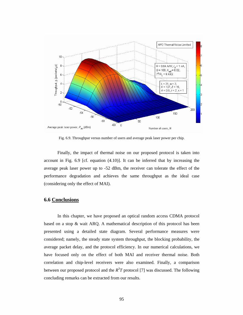
95
Fig. 6.9. Throughput versus number of users and average peak laser power per chip.
Finally, the impact of thermal noise on our proposed protocol is taken into
account in Fig. 6.9 [cf. equation (4.10)]. It can be inferred that by increasing the
average peak laser power up to -52 dBm, the receiver can tolerate the effect of the
performance degradation and achieves the same throughput as the ideal case
(considering only the effect of MAI).
6.6 Conclusions
In this chapter, we have proposed an optical random access CDMA protocol
based on a stop & wait ARQ. A mathematical description of this protocol has been
presented using a detailed state diagram. Several performance measures were
considered; namely, the steady state system throughput, the blocking probability, the
average packet delay, and the protocol efficiency. In our numerical calculations, we
have focused only on the effect of both MAI and receiver thermal noise. Both
correlation and chip-level receivers were also examined. Finally, a comparison
between our proposed protocol and the R3T protocol [7] was discussed. The following
concluding remarks can be extracted from our results.

96
1- The performance of the proposed CDMA protocol using correlation receivers
is nearly close to that of the R3T protocol with chip-level receivers.
2- The proposed protocol outperforms the R3T protocol (in terms of the system
throughput and average packet delay) in high population networks, whereas
for smaller size networks the R3T protocol slightly outperforms the proposed
one.
3- Both protocols exhibit satisfactory blocking probability only for small traffic
loads. Furthermore, the average packet delay is acceptable under different
network parameters.
4- For larger interstation distances, the proposed protocol accommodates a higher
number of users. Also the quality of service (QOS) requirements can be
achieved in a larger dynamic range (wider range of users).
5- Our proposed protocol provides an improvement in the protocol efficiency for
both small and large population networks. Also it is clear that for an
interstation distance m 200=z , the efficiency of our protocol with 70=N is
as good as the efficiency of the R3T protocol with 30=N .
6- We can tolerate the effect of thermal noise by reasonably increasing the
average peak power at the transmitter to -52 dBm, [37].
7- The complexity of the proposed protocol is significantly reduced compared to
the R3T protocol. Also the cost is reduced when using correlation receivers.

CHAPTER 7
CONCLUSIONS AND FUTURE WORK
Outline:
• Conclusions
• Future Research Avenues

97
CHAPTER 7
CONCLUSIONS AND FUTURE WORK
7.1 Conclusions
In this thesis, we have first reviewed previous work on optical CDMA
communication systems. Both physical layer and data link layer of slotted optical
CDMA packet networks have been considered. By studying the performance of
different optical CDMA receiver structures, we have found out that for a large number
of active users in the network and for the same set of spreading codes, the effect of
MAI becomes considerable and thus, the performance of these receivers is
significantly reduced. There emerges a high need to design a robust data link layer
and MAC protocols for optical CDMA networks that ensure a fair access to the
network environment.
In this work, we have focused mainly on random access protocols and
solutions for LANs, but many of the principles can also be used for access networks.
A physical star topology is used in our optical CDMA network. Compared to ring and
bus topologies, star networks offer a better optical power budget and are easy to
install, configure, manage, and troubleshoot. Optical orthogonal codes (OOCs) with
correlation constraints set to one have been used as the users’ signature codes to
ensure minimal interference level. Optical direct-detection CDMA and binary on-off
keying (OOK) have been implemented at the physical layer.
Most studies of optical CDMA use simple channel models where noise and
dispersion are neglected. One of the main objectives of this research was to study a
model where both thermal noise and dispersion, are taken into account. In Chapter 4,
the Gaussian approximation has been used to study the effect of thermal noise on the
performance of the round robin receiver/transmitter (R3T) protocol. Also the impact of
the dispersion on limiting the user bit rate has been also considered. We have proved
by numerical analysis that the effect of thermal noise dominates the performance only
for the case of low population networks, whereas the effect of MAI becomes
dominant for larger networks. The power penalty to be paid to overcome the
degradation in the performance has also been calculated.

98
Also in this thesis we have suggested a queuing model for the R3T protocol in
order to enhance its performance especially at large population networks and at high
traffic loads. This is because in the R3T protocol it was assumed that each node is
equipped with only a single buffer to store only the message being served. Any arrival
to a non empty buffer was discarded; this of course gave rise to a high blocking
probability. In Chapter 3, we have derived an expression for the blocking probability
and demonstrated that the blocking probability can reach as high as 95% under certain
network conditions. A detailed state diagram for this modified R3T protocol has been
presented in Chapter 5 and has been analyzed using the equilibrium point analysis
(EPA) technique. Our results revealed that significant improvement in the steady state
system throughput and the protocol efficiency can be achieved by only adding a single
buffer to the system which does not add significantly to the network’s complexity.
Furthermore, the R3T protocol with a queuing subsystem exhibits an acceptable
timeout probability under different network parameters.
Finally, we have proposed an optical random access CDMA protocol based on
stop & wait ARQ in Chapter 6. A mathematical description of this protocol has been
outlined using a detailed state diagram. Several performance measures have been
considered; namely, the steady state system throughput, the blocking probability, the
average packet delay, and the protocol efficiency. The performance has been also
examined for both correlation and chip-level receivers. We have proved by numerical
analysis that the proposed protocol is less complex and significantly outperforms the
R3T protocol which is based on a go-back n technique. Our results have also showed
that the performance of the proposed protocol with correlation receivers is nearly
close to that of the R3T protocol with chip-level receivers, which reduces the overall
system cost.
7.2 Future Research Avenues
Although the objectives of this research have been achieved, it would be
interesting to see some of the aspects discussed in this thesis implemented in an
experimental set-up. Any experimental results can then be fed back to the simulation
model for further performance optimization and validation. Below, we present several
directions for future research in the area of optical CDMA networks.

99
• The design and evaluation of hybrid MAC protocols where nodes apply
different protocols according to the current traffic load.
• Channel load sensing protocols (CLSP) and packet avoidance collision (PAC)
protocols can be applied.
• The combination of error correction and traffic control by MAC can be studied
for further improvement in the performance of optical CDMA networks.
• Studying optical random access CDMA protocols with larger buffers.
• Two dimensional codes may be implemented to provide larger code sets with
lower interference levels.
• Power control depending on the number of active users in the network may be
used to compensate for the effect of thermal noise. The effect of shot noise and
beat noise can also be included.

REFERENCES

100
REFERENCES
[1] Rajiv Ramaswami, “Optical fiber communication: from transmission to
network,” IEEE comm. magazine, 50th anniversary commemorative issue, pp.
138-147, May 2002.
[2] A. Stok, and E. H. Sargent, “System performance comparison of optical
CDMA and WDMA in a broadcast local area network,” IEEE Comm. Lett.,
vol. 6, No. 9, pp. 409-411, September 2002.
[3] A. Stok, and E. H. Sargent, “Comparison of utilization in optical CDMA and
WDMA broadcast local-area networks with physical noise,” IEEE
International conference on communications (ICC), 2003.
[4] C.-S. Hsu, and V. O. K. Li, “Performance analysis of slotted fiber-optic code-
division multiple-access (CDMA) packet networks,” IEEE Trans. Comm., vol.
COM-45, pp. 819-828, July 1997.
[5] C.-S. Hsu, and V. O. K. Li, “Performance analysis of unslotted fiber-optic
code-division multiple-access (CDMA) packet networks,” IEEE Trans. Comm.,
vol. COM-45, pp. 978-987, August 1997.
[6] H. M. H. Shalaby, “Optical CDMA random access protocols with and without
pretransmission coordination,” IEEE/OSA J. Lightwave Technol., vol. LT-21,
pp. 2455-2462, November 2003.
[7] H. M. H. Shalaby, “Performance analysis of an optical CDMA random access
protocol,” IEEE/OSA J. Lightwave Technol., vol. LT-22, pp. 1233-1241, May
2004.
[8] M. A. A. Mohamed, H. M. H. Shalaby, and E. A. El-Badawy, “Optical CDMA
protocol with selective retransmission,” in Proc. Ninth IEEE Symp. Computers
and Communications (ISCC 2004), Alexandria, Egypt, pp. 621-626, June 29 -
July 1, 2004.
[9] F. R. Chung, J. A. Salehi, and V. K. Wei, “Optical orthogonal codes: Design,
analysis, and applications,” IEEE Trans. Inform. Theory, vol. 35, pp. 595-604,
May 1989.

101
[10] J. A. Salehi, “Code division multiple-access techniques in optical fiber
networks - Part I: Fundamental principles,” IEEE Trans. Comm., vol. 37, pp.
824-833, August 1989.
[11] J. A. Salehi, and C. A. Brackett, “Code division multiple access techniques in
optical fiber networks - Part II: System performance analysis,” IEEE Trans.
Comm., vol. 37, No. 8, pp. 834-842, August 1989.
[12] K. Iversen, and D. Hampicke, “Comparison and classification of all-optical
CDMA systems for future telecommunication networks,” SPIE Proc., vol.
2614, pp. 110-121, October 1995.
[13] J. Y. Hui, “Pattern code modulation and optical decoding - A novel code-
division multiplexing technique for multifiber networks,” IEEE Journal on
Selected Areas in Comm., vol. SAC-3, No. 6, pp. 916-927, November 1985.
[14] P. R. Prucnal, M. A. Santoro, and T. R. Fan, “Spread spectrum fiber-optic local
area network using optical processing,” IEEE/OSA J. Lightwave Technol., vol.
LT-4, No. 5, pp. 547-554, May 1986.
[15] P. R. Prucnal, M. A. Santoro, and S. K. Sehgal, “Ultrafast all-optical
synchronous multiple access fiber optical networks,” IEEE Journal on Selected
Areas in Communications, vol. SAC-4, No. 9, pp. 1484-1493, December 1986.
[16] M. Kavehrad, and D. Zaccarin, “Optical code-division-multiplexed systems
based on spectral encoding of noncoherent sources", IEEE/OSA J. Lightwave
Technol., vol. 13, No. 3, pp. 534-545, March 1995.
[17] H. Fathallah, L. A. Rusch, and S. LaRochelle, “Passive optical fast frequency-
hop CDMA communications system,” IEEE/OSA J. Lightwave Technol., vol.
17, No. 3, pp. 397-405, March 1999.
[18] H. M. H. Shalaby, “Complexities, error probabilities, and capacities of optical
OOK-CDMA communication systems,” IEEE Trans. Comm., vol. 50, No. 12,
pp. 2009-2017, December 2002.
[19] S. Zahedi, and J. A. Salehi, “Analytical comparison of various fiber-optic
CDMA receiver structures,” IEEE/OSA J. Lightwave Technol., vol. LT-18, pp.
1718-1727, December 2000.

102
[20] D. V. Sarwate, and M. B. Pursley, “Crosscorrelation properties of
pseudorandom and related sequences,” Proc. IEEE, vol. 68, pp. 593-619,
May 1980.
[21] A. A. Shaar, and P. A. Davies, “Prime sequences: Quasi-optimal sequences for
OR channel code division multiplexing,” IEEE Electronics Letters, vol. 19, No.
21, pp. 888-889, 13 October 1983.
[22] L. Nguyen, B. Aazhang, and J.F. Young, “All-optical CDMA with bipolar
codes,” IEEE Electronics Letters, vol. 31, No. 6, pp. 469-470, 16 March 1995.
[23] R. M. H. Yim, L. R. Chen, and J. Bajcsy, “Design and performance of 2-D
codes for wavelength-time optical CDMA,” IEEE Photonics Technology
Letters, vol. 14, No. 5, pp. 714-716, May 2002.
[24] R. M. H. Yim, J. Bajcsy, and L. R. Chen, “A new family of 2-D wavelength-
time codes for optical CDMA with differential detection,” IEEE Photonics
Technology Letters, vol. 15, No. 1, pp. 165-167, January 2003.
[25] T. Ohtsuki, “Performance analysis of direct-detection optical asynchronous
CDMA systems with double optical hard-limiters,” IEEE/OSA J. Lightwave
Technol., vol. LT-15, pp. 452-457, March 1997.
[26] H. M. H. Shalaby, “Chip-level detection in optical code-division multiple-
access,” IEEE/OSA J. Lightwave Technol., vol. LT-16, pp. 1077-1087,
June 1998.
[27] M. Azizoglu, J. A. Salehi, and Y. Li, “Optical CDMA via temporal codes,”
IEEE Trans. Comm., vol. 40, pp. 1162-1170, July 1992.
[28] J. Muchenheim, and D. Hampicke, “Protocols for optical CDMA local area
networks” Proc. NOC'97, (Antwerpen), vol. 1, pp. 255-262, 1997
[29] L. Lenzini, J. O. Limb, W. W. Lu, I. Rubin, and M. Zukerman, “Analysis and
synthesis of MAC protocols,” IEEE Journal on Selected Areas in
Communications, vol. 18, No. 9, pp. 1557-1561, November 2000.
[30] P. Kamath, J. Touch, and J. Bannister, “The need for media access control in
optical CDMA networks,” Proc. IEEE Infocom, 2004.
[31] N. Mehravari, “Performance and protocol improvements for very high speed

103
optical fiber local area networks using a passive star topology,” IEEE/OSA J.
Lightwave Technol, vol. LT-8, pp. 520-530, April 1990.
[32] H. Takagi, and L. Kleinrock, “Throughput analysis for persistent CSMA
systems,” IEEE Trans. Comm., vol. COM-33, No. 7, pp. 627-638, July 1985.
[33] William Stallings, Data and Computer Communications, New York: 6th
edition, Prentice Hall, 2000.
[34] G. P. Agrawal, Fiber-optic Communication Systems, New York: 3rd edition,
John Wiley & Sons, Inc., 2002.
[35] B. Mukherjee, Optical Communication Networks, New York: McGraw-Hill,
1997.
[36] E. K. H. Ng, G. E. Weichenberg, and E. H. Sargent, “Dispersion in
multiwavelength optical code-division multiple-access systems: Impact and
remedies,” IEEE Trans. Comm., vol. 50, No. 11, November 2002.
[37] Z. A. El-Sahn, Y. M. Abdel-Malek, H. M. H. Shalaby, and El-S. A. El-
Badawy, "Performance limitations in the R3T optical random access CDMA
protocol," Submitted for possible publication to OSA J. Optical Networking,
March 2005.
[38] V. F. B. Mezger, and M. B. Pearce, “Dispersion limited fiber-optic CDMA
systems with overlapped signature sequences,” in Proc. IEEE Laser and
Electro-Optics Soc. 9th Annu. Meeting, pp. 408-409, 1996.
[39] T. Pfeiffer, M. Witte, and B. Deppisch, “High-speed transmission of broadband
thermal light pulses over dispersive fibers,” IEEE Photon. Technol. Lett., vol.
11, pp. 385-387, March 1999.
[40] M. J. Karol, “Performance of the PAC optical packet network,” IEEE/OSA J.
Lightwave Technol., vol 11. No. 8, pp. 1394-1399, August 1993.
[41] H. M. H. Shalaby, “Effect of thermal noise and APD noise on the performance
of OPPM-CDMA receivers,” IEEE/OSA J. Lightwave Technol., vol. 18, No. 7,
pp. 905-914, July 2000.
[42] Z. A. El-Sahn, Y. M. Abdel-Malek, H. M. H. Shalaby, and El-S. A. El-
Badawy, "The R3T optical random access CDMA protocol with queuing

104
subsystem," Submitted for possible publication to the IEEE/OSA J. Lightwave
Technol., also a summary submitted to the 31st European Conference on
Optical Communication, (ECOC 2005), Glasgow, Scotland, 25-29 September
2005.
[43] J. R. Sack, and J. Urrutia, Handbook of Computational Geometry, North
Holland: Elsevier Science, 2000.
[44] Xi Zhang, and Kang G. Shin, "Markov-chain modeling for multicast signaling
delay analysis", IEEE/ACM Transactions on Networking, vol. 12, No. 4, pp.
667-680, August 2004.

جامعة اإلسكندرية آلية الهندسة
للشبكات الضوئية عشوائيةبروتوآوالت الوصولية ال يالمستقبلية ذات الوصولية المتعددة بالتـقسيم الشفر
رسالة مقدمة استيفاء جزئيا لمتطلبات الحصول على
درجة الماجستير
في
الهندسة الكهربية
من المهندس
أحمد رشاد الصحنزياد
تحت اشراف
يحسام محمد حسان شلب. د. أيالسيد عبد المعطى البدو. د.أ
٢٠٠٢سبتمبر : مسجلة في ٢٠٠٥ ابريل: مقدمة في

بسم اهللا الرحمن الرحيم
يالملخص العرب
رين دين األخي ى العق رة ف ة آبي ضؤية أهمي اف ال صاالت باأللي سبت االت ادة اآت را للزي ك نظ و ذل
ردد وئ فى آمية البيانات المطلوب نقلها، حيث تتمتع األلياف الض مطردةال دا يية بنطاق ت واسع ج
ذا النطاق .شرات التيراهرتزئقة تصل الى عيمكنها من نقل البيانات بمعدالت فا تفادة من ه و لالس
ددة يالتردد ات الوصولية المتع . Multiple Access Techniques الواسع يجب استخدام احدى تقني
شفر سيم ال ددة بالتق هى Code Division Multiple Access (CDMA) يتعد تقنية الوصولية المتع
ل س تفادة، بجانب ـالطريقة المثلى لتحقيق هذه االس ذ العمل ـتمتعها بمميزات أخرى مث يـهولة التنفي
.و امكانية تغيير عدد المشترآين فى الشبكة بسهولة
شفر ية ذات وئيتعرض هذا البحث لدراسة الشبكات الض سيم ال ددة بالتق ى آل يالوصولية المتع عل
ة ييمن مستو ة المادي ات Physical Layer الطبق ة وصلة البيان م Data Link Layer و طبق حيث ت
-:الترآيز على البروتوآوالت المستخدمة فى الشبكات الوصولية و المحلية و هما
.Random Access Protocols بروتوآوالت الوصولية العشوائية -
.Media Access Control (MAC) Protocols صولية الوسائطيةوبروتوآوالت تحكم ال -
الة بدراس دأ الرس أثير لة ـتب شت ضوضاء و الت ضوئـال تقباليتت ال ول االس ى أداء بروتوآ عل
ال ي و االرس لوب الحلق ح Round Robin Receiver/Transmitter Protocol باألس ، و توض
ى أداء البروتوآول فى شبكات يغلبالنتائج الرقمية أن تأثير الضوضاء الحرارية االتصاالت عل
ا من اذات األعداد الصغيرة داخل الوصول ايغلب لمشترآين، بينم دد يلت Multiple Access المتع
Interference (MAI) ش ا ـ على األداء فى ال ر حجم م حس . بكات األآب ا ت ة ـآم درة المثالي يم الق اب ق
وج ول الم سلب يو الط أثير ال ى الت ب عل ة ي المناسب للتغل ضوضاء الحراري ن ال ل م شتت لك والت
. فى األلياف الضوئيةيالضوئ
وذ افة نم ة اض م دراس صفيفت ول Queuing Model ج ت ى بروتوآ ال ال تقبال و االرس االس
د الحادث باألسلوب الحلقي ى الفق ائل، ا في بهدف تحسين األداء و ذلك عن طريق التغلب عل لرس
ة . لتخزين الرسائل اضافية وحدةزيادة تحيث تم State Diagram تم وضع تصور لمخطط الحال
زن يباستخدام طريقة التحليل النقط لتنفيذ هذه الدراسة و تحليله تفصيليا Equilibrium Point المت

Analysis . ة ا فائق اأوضحت النتائج تحسن ة، و خاصة فى حال صفة عام شبكات ذات فى األداء ب ال
. األحمال المرورية العاليةذات المشترآين و منالكبيرة عداداأل
مع الحفاظ على أدائه أو تحسينه باألسلوب الحلقي بروتوآول االستقبال و االرسال من أجل تبسيط
ة قف و انتظر ـوائيـولية عش ـتم اقتراح بروتوآول وص ى طريق د عل د يعتم ،Stop & Wait ة جدي
و ة التعامل مع الرسائل التى تحت ى يو بدراسة آليات االتصال بين المرسل و المستقبل و آيفي عل
تقبالها آذا وData Packets أآثر من حزمة بيانات تم اس م ي ات التى ل آيفية التعامل مع حزم البيان
ن األداء ال م ستو ع ع بم رح يتمت ول المقت ائج أن البروتوآ رت النت اح أظه ك بنج ة و ذل مقارن
ى باألسلوب الحلقي االستقبال و االرسال بروتوآول ب ى عالوة عل ه عل ر مقدرت استيعاب عدد أآب
.من المشترآين
-:ية أبواب آالتالتتكون هذه الرسالة من سبع
ة :الباب األول ضمقدم اف ال صاالت باأللي ة االت اول أهمي شبكات ذات وئ تتن ة ال ية و خاص
ذا ل يلي ذلك عرض ي، بالتقسيم الشفر المتعددة الوصولية مساهمة الباحث في ه
. المختلفة للنقاط البحثية الرئيسية بأبواب الرسالةابرازالمجال و
فى أنظمة االتصاالت ي بالتقسيم الشفر المتعددة الوصوليةذات عرض للتقنيات :الباب الثانى
ضوئية ة ،ال ا ل و دراس ة بينه ستقبالت و المقارن ة للم واع المختلف ث ألن ن حي م
.األداء و مستوى التعقيد
والت :الباب الثالث ى بروتوآ سابقة ف ات ال ص للدراس وليملخ ش الوص وائيةـة الع
م و والت تحك ائطيةوالبروتوآ يصولية الوس ستخدمة ف ضوئية الم شبكات ال ال
.ي بالتقسيم الشفر المتعددةالوصوليةذات
ة :الباب الرابع ذا دراس ضوئية وآ شبكات ال ن أداء ال د م ى تح ل الت صر للعوام عرض مخت
ضوئ ل شتت ال ة والت ى أداء يتأثير الضوضاء الحراري ضوئية عل اف ال فى األلي
ول تقبال و االربروتوآ ال االس يس لوب الحلق م باألس م ث ى ت ائج الت عرض النت
.الحصول عليها
ة أداء :الباب الخامس ال دراس تقبال و االرس ول االس يبروتوآ لوب الحلق افة باألس د اض بع
ادة تلرسائل، حيث تم ا فيلتغلب على الفقد الحادث لو ذلك نموذج تصفيف زي

افية دة اض ائل وح زين الرس م ، لتخ رض ث م ل ع ى ت ائج الت ا لنت صول عليه الح
.و مقارنتها بالنتائج السابقة
ه عرض اقتراح لبروتوآول جديد يعتمد على طريقة قف و انتظر و دراسة أدا :الباب السادس ئ
اط ستقبل االرتب ن الم ل م تخدام آ ستقبل Correlation Receiver يباس و م
ذاذة ستوى الج ه ب وChip-Level Receiverم تقب مقارنت ول االس البروتوآ
.نتائج الدراسةل أخيرا عرض وباألسلوب الحلقيو االرسال
دم عرض لخالصة ما تم دراسته والنتائج التي :الباب السابع رح المق ا، والمقت تم التوصل اليه
.للتطوير في مجال نقل المعلومات باأللياف الضوئية